
Synchronous generator and frequency converter
in wind turbine applications:
system design and efficiency
Anders Grauers
Technical Report No. 175 L
1994
ISBN 91-7032-968-0

Synchronous generator and frequency converter
in wind turbine applications:
system design and efficiency
by
Anders Grauers
Technical report No. 175 L
Submitted to the School of Electrical and Computer Engineering
Chalmers University of Technology
in partial fullfillment of the requirements
for the degree of
Licentiate of Engineering
Department of Electrical Machines and Power Electronics
Chalmers University of Technology
Göteborg, Sweden
May 1994

1
Abstract
This report deals with an electrical system for variable-speed wind power
plants. It consists of a synchronous generator, a diode rectifier and a
thyristor inverter. The aim is to discuss the system design and control, to
model the losses and to compare the average efficiency of this variable-speed
system with the average efficiency of a constant-speed and a two-speed
system. Only the steady state operation of the system is discussed. Losses in
the system are modelled, and the loss model is verified for a 50 kVA
generator. The proposed simple loss model is found to be accurate enough to
be used for the torque control of a wind turbine generator system. The most
efficient generator rating is discussed, and it is shown how the voltage control
of the generator can be used to maximize the generator and converter
efficiency. The average efficiency of the system is calculated. It depends on
the median wind speed of the turbine site. It is found that a variable-speed
system, consisting of a generator and a converter, can have an average
efficiency almost as high as a constant-speed or a two-speed system. Three
different control strategies and their effect on the system efficiency are
investigated.
Acknowledgement
I would like to thank my supervisor, Dr Ola Carlson, for his support in this
research project. Also my examinator Dr Karl-Erik Hallenius, Professor
Jorma Luomi and Professor Kjeld Thorborg have given me valuable
comments and suggestions during the work on this report. Further, I would
like to thank Margot Bolinder for linguistic help.
The financial support for this project is given by the Swedish National Board
for Industrial and Technical Development (NUTEK) and it is gratefully
acknowleged.

2
List of contents
Abstract..........................................................................................................................
1
Acknowledgement.........................................................................................................
1
List of contents..............................................................................................................
2
List of symbols ..............................................................................................................
4
1 Introduction ................................................................................................................
6
1.1 Description of variable-speed generator systems...........................
7
1.1.1 Synchronous generator and diode-thyristor
converter.......................................................................................
7
1.1.2 Generators and rectifiers...........................................................
8
1.1.3 Inverters.....................................................................................
11
1.2 Wind turbine characteristics.............................................................
13
1.3 Variable-speed wind turbines............................................................
15
1.4 A design example system...................................................................
15
2 The synchronous generator system ....................................................................
16
2.1 The control system..............................................................................
17
2.2 The generator .......................................................................................
19
2.2.1 Speed rating ...............................................................................
19
2.2.2 Current rating............................................................................
20
2.2.3 Voltage rating ............................................................................
21
2.2.4 Other aspects of the rating.....................................................
22
2.2.5 Generator rating........................................................................
23
2.2.6 Generator efficiency .................................................................
24
2.2.7 Design example..........................................................................
25
2.3 Rectifier..................................................................................................
27
2.3.1 Diode commutation...................................................................
27
2.3.2 Equivalent circuit......................................................................
28
2.3.3 Design example..........................................................................
30
2.4 Dc filter ..................................................................................................
31
2.4.1 Filter types.................................................................................
32
2.4.2 Harmonics in the dc link..........................................................
34
2.4.3 Smoothing reactor of the diode rectifier................................
35
2.4.4 Smoothing reactor of the inverter .........................................
38
2.4.5 Dc capacitance..........................................................................
42
2.4.6 Resonance damping..................................................................
42
2.4.7 Dc
filter for the design example system ...............................
43
2.5 Inverter..................................................................................................
46
2.5.1 Inverter pulse number.............................................................
47
2.5.2 Protection circuits.....................................................................
49
2.5.3 Design example..........................................................................
50
3 Model of generator and converter losses.............................................................
51
3.1 Model of machine losses......................................................................
51
3.1.1 Friction and windage loss torque............................................
52
3.1.2 Core losses..................................................................................
53
3.1.3 Winding losses............................................................................
55

3
3.1.4 Exciter losses.............................................................................
56
3.1.5 Additional losses........................................................................
57
3.1.6 Complete generator loss model.............................................
58
3.1.7 Calculating the generator flux ..............................................
59
3.1.8 Estimating the field current..................................................
60
3.1.9 Parameters for the generator loss model ...........................
61
3.1.10 Errors of the generator model...............................................
63
3.1.11 Error in the windage and friction losses..............................
63
3.2 Model of the converter losses ............................................................
69
3.3 Model of the gear losses......................................................................
70
3.4 Verification of the generator loss model..........................................
70
3.4.1 The laboratory system............................................................
71
3.4.2 Parameters of the laboratory system .................................
72
3.4.3 Verification of the exciter losses............................................
81
3.4.4 Model error at resistive load...................................................
81
3.4.5 Model error at diode load..........................................................
84
3.4.6 Error in the torque control......................................................
85
3.5 Model for the 300 kW design example .............................................
87
3.5.1 Generator parameters.............................................................
87
3.5.2 Converter parameters.............................................................
89
3.5.3 Gear parameters ......................................................................
89
4 The use of the loss model in control and design..................................................
90
4.1 Optimum generator voltage control.................................................
90
4.2 Efficiency as a function of generator size........................................
92
4.3 Optimum generator speed .................................................................
94
5 Comparison of constant and variable speed......................................................
99
5.1 The per unit turbine model.................................................................
99
5.2 Power and losses as functions of the wind speed.........................
101
5.2.1 Assumptions for the power functions ................................
101
5.2.2 Power functions ......................................................................
105
5.2.3 Turbine power .........................................................................
107
5.2.4 Gear losses...............................................................................
108
5.2.5 Generator and converter losses...........................................
108
5.2.6 Losses at different voltage controls....................................
109
5.2.7 Produced electric power.........................................................
110
5.3 Energy and average efficiency........................................................
111
5.3.1 Assumptions for the energy calculations..........................
112
5.3.2 Wind energy captured by the turbine.................................
114
5.3.3 Gear energy output and average gear
efficiency ..................................................................................
114
5.3.4 Electric energy and average electric efficiency................
115
5.3.5 Total efficiency including the gear.......................................
118
5.3.6 Produced energy......................................................................
119
5.4 Summary of average efficiency comparison................................
121
6 Conclusions............................................................................................................
123
7 References..............................................................................................................
124

4
List of symbols
Quantities
B
Magnetic flux density
C
Capacitance
d
Turbine diameter
E
Induced voltage
e
Per unit induced voltage
f
Frequency
I
Current
i
Per unit current
L
Inductance
n
Rotational speed
n'
Per unit rotational speed
P
Power
p
Per unit power
R
Resistance
r
Per unit resistance
S
Apparent power
T
Torque
t
Per unit torque
U
Voltage
u
Per unit voltage
v
Per unit wind speed
X
Reactance
x
Per unit reactance
Z
Impedance
α
Firing angle of the inverter
η
Efficiency
λ
Tip speed ratio of the turbine
ω
Electrical angular frequency
Ψ
Flux linkage
ψ
Per unit flux linkage
Constants and components
C
Constant, coefficient
Th
Thyristor
VDR
Voltage depending resistor (ZnO)

5
Indices for parts of the system:
a
Armature
c
Converter
d
Dc link
E
Exciter
f
Field
g
Generator
gear
Gear
i
Inverter
net
Network
r
Rectifier
rotor
Rotor
t
Turbine
to
Turn-off circuit
damp
Damper circuit
Other indices:
ad
Additional losses
b
Base value
com
Commutation
Cu
Copper losses
d axis
D-axis of the synchronous generator
diode
Diode loaded
est
Estimated value
Fe
Core losses
Ft
Eddy current losses
Hy
Hysteresis losses
lim
Limit value
loss
Losses
max
Maximum value
mesh
Gear mesh (losses)
min
Minimum value
N
Rated value
opt
Optimum
P
Power (-Coefficient)
p-p
Peak-to-peak value
q axis
Q-axis of the synchronous generator
ref
Reference value
res
Resistively loaded
s
Synchronous (reactance)
ss
Standstill
tot
Total
(k)
kth harmonic
(1)
Fundamental component
0
No load
µ
Friction
σ
Leakage

6
1 Introduction
In the design of a modern wind turbine generator system, variable speed is
often considered. It can increase the power production of the turbine by about
5 %, the noise is reduced and forces on the wind turbine generator system can
be reduced. Its major drawbacks are the high price and complexity of the
converter equipment.
This report deals with a variable-speed system consisting of synchronous
generator, diode rectifier and thyristor inverter. The advantages of the
synchronous generator and a diode rectifier are the high efficiency of the
rectifier and the low price. There are two disadvantages that can be
important in wind turbine generator systems. Motor start of the turbine is
not possible without auxiliary equipment and the torque control is normally
not faster than about 8 Hz [1]. The aim of this report is to describe an
efficient variable-speed system and to model the generator and converter
losses. The loss model is intendend to be used for steady state torque control
and to maximize the system efficiency.
The synchronous generator system has been investigated earlier. Ernst [1],
for example, describes the system possibilities by presenting various system
configurations, methods for modelling and control strategies. Hoeijmakers
derives an electric model for the generator and converter [2] and a simplified
model intended for control use [3], not including the effects of ripple and
harmonics. Carlson presents a detailed model for the simulation of the
generator and converter system by numerical solution of the equations [4].
This report focuses on system design, modelling of the system losses,
maximizing the efficiency and calculation of average efficiency. To be able to
find reasonable parameters for the loss model, the generator rating as well as
the converter design are discussed in Chapter 2. In Chapter 3, the loss model
is derived and compared with measurments. In Chapter 4, the generator
voltage control is optimized and the influence of the generator rating on the
system efficiency is discussed. A comparison is made between the losses and
average efficiency of a variable-speed, a constant-speed and a two-speed
system in Chapter 5. The report deals only with the steady-state behaviour
of the system.
7
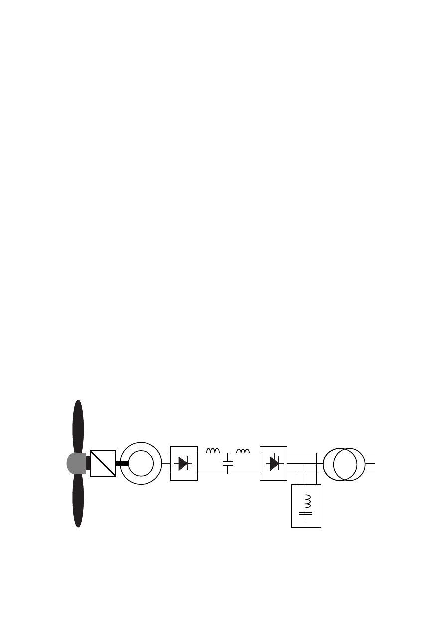
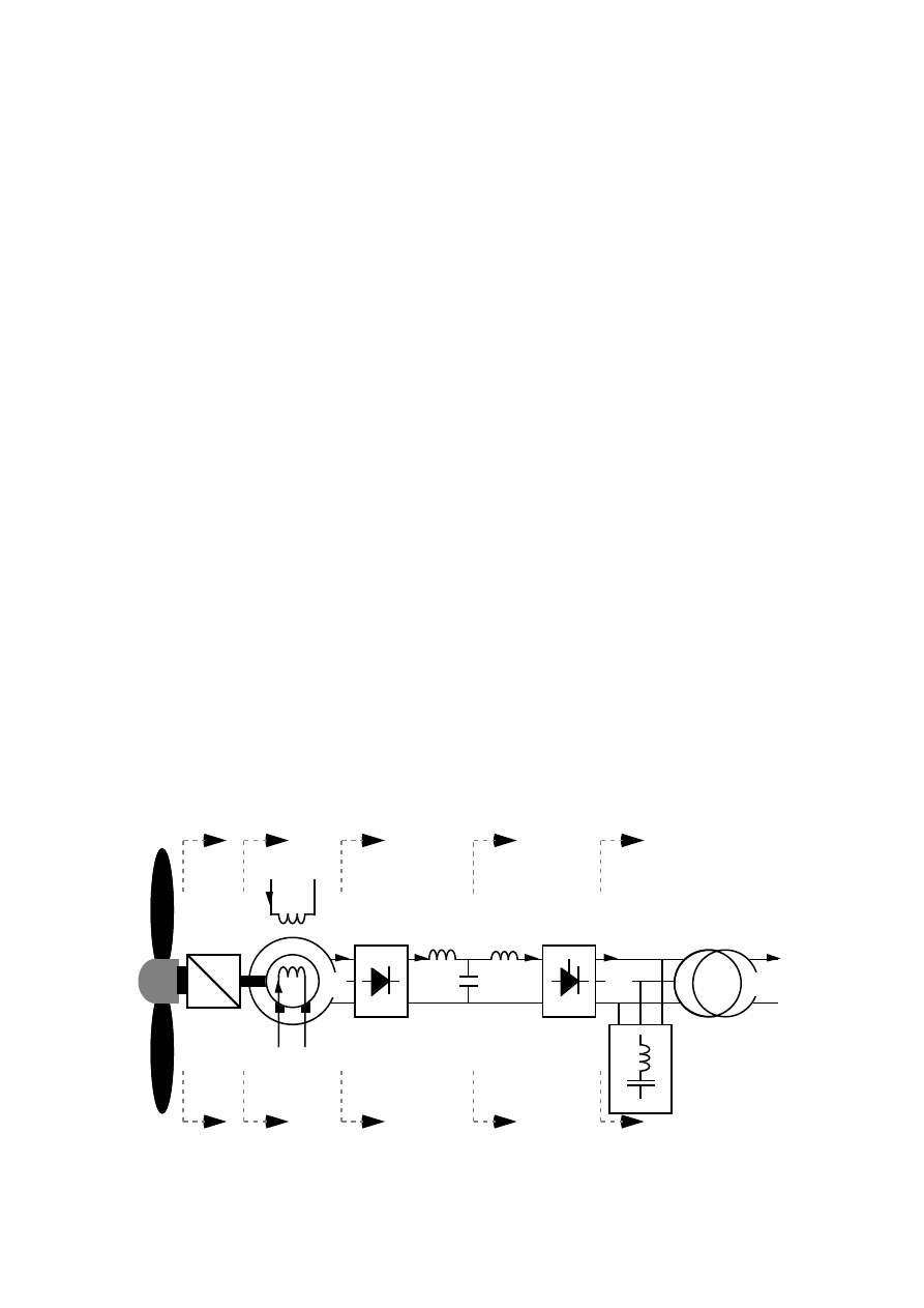
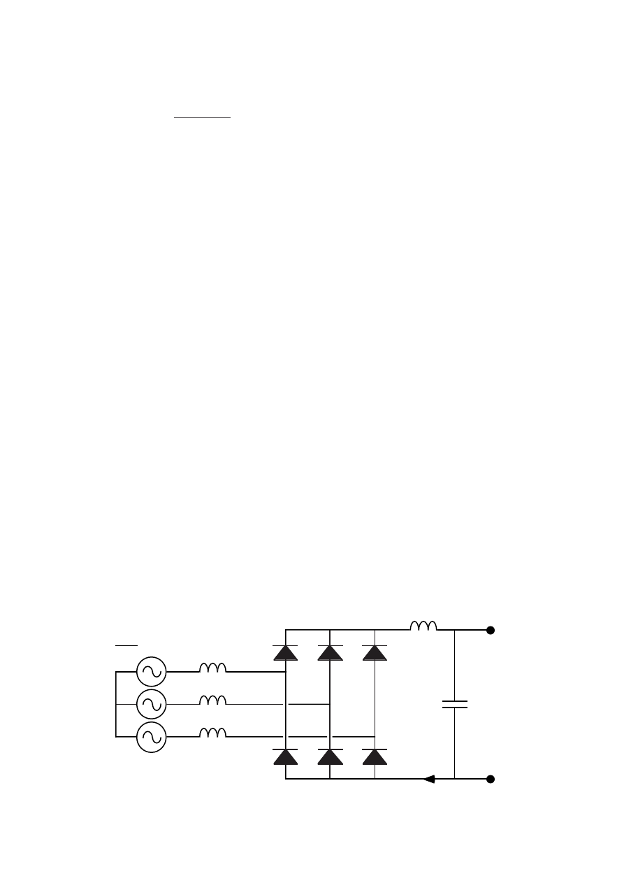
1.1 Description of variable-speed generator systems
1.1.1 Synchronous generator and diode-thyristor converter.
The generator system discussed in this report is a system consisting of a
synchronous generator, a diode rectifier, a dc filter and a thyristor inverter.
The inverter may have a harmonic filter on the network side if it is necessary
to comply with utility demands. The harmonic filter is, however, not included
in the efficiency calculations in this report. Figure 1.6 shows the total power-
generating system.
The advantage of a synchronous generator is that it can be connected to a
diode or thyristor rectifier. The low losses and the low price of the rectifier
make the total cost much lower than that of the induction generator with a
self-commutated rectifier [5]. When using a diode rectifier the fundamental of
the armature current has almost unity power factor. The induction generator
needs higher current rating because of the magnetization current.
The disadvantage is that it is not possible to use the main frequency
converter for motor start of the turbine. If the turbine cannot start by itself it
is necessary to use auxiliary start equipment. If a very fast torque control is
important, then a generator with a self-commutated rectifier allows faster
torque response. A normal synchronous generator with a diode rectifier will
possibly be able to control the shaft torque up to about 10 Hz, which should
be fast enough for most wind turbine generator systems.
Gear
Synchronous
generator
Wind turbine
Diode
rectifier
Dc-filter
Thyristor
inverter
Harmonic
filter
Network
transformer
Figure 1.6
The proposed generator and converter system for a wind turbine
generator system.

8
The armature current of a synchronous generator with a diode rectifier can
be instable. This instability can, according to Hoeijmakers, be avoided by
using a current-controlled thyristor rectifier [3]. However, using a thyristor
rectifier is much more expensive than using a diode rectifier and it also makes
it neccesary to use a larger generator. Therefore, a diode rectifier should be
used if the rectifier current can be controlled by other means. That is possible
by means of the inverter current control. The control may, however, be
slightly slower than that of a thyristor rectifier.
Enclosed generators (IP54) are preferred in wind turbine generator systems.
But standard synchronous generators are usually open (IP23) and cooled by
ambient air ventilated through the generator. Enclosed synchronous
generators are manufactured, but they can be rather expensive. Open
generators can maybe be used if the windings are vacuum-impregnated.
Standard induction generators, with a rated power up to at least 400 kW, are
enclosed.
A thyristor inverter is used in the system investigated in this report, mainly
because it is available as a standard product at a low price and also for high
power. In the future, when the size of the transistor inverters is increased and
the price reduced, they will be an interesting alternative to the thyristor
inverter.
1.1.2 Generators and rectifiers
In this section different generators for variable-speed systems are compared.
A cage induction generator is normally used together with a self-commutated
rectifier because it must be magnetized by a reactive stator current. The
self-commutated rectifier allows a fast torque control but it is much more
expensive than the diode rectifier and it is less efficient. An alternative to the
expensive self-commutated rectifier would be an induction generator
magnetized by capacitors and feeding a diode rectifier. The disadvantages of
that system are that the generator iron core must be saturated to stabilize
the voltage, which leads to a poor efficiency, and the capacitance value must
be changed with the generator speed. The two different cage induction
generator and rectifier combinations are shown in Figure 1.1.
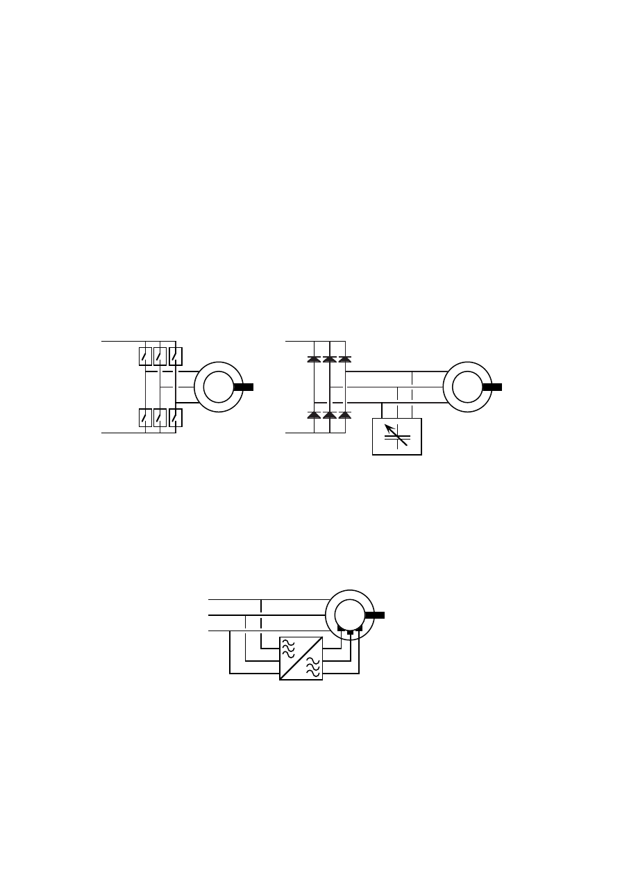
9
An induction generator and a rotor cascade has the stator connected directly
to the network and the rotor windings are connected to the network via a
frequency converter, see Figure 1.2. This system is interesting mainly if a
small speed range is used because then the frequency converter can be
smaller than in the other systems. A speed range of
±
20 % from the
synchronous speed can be used with a frequency converter rated only about
20 % of the total generator power. The main part of the power is transferred
by the stator windings directly to the network. The rest is transferred by the
frequency converter from the rotor windings. The disadvantage of this system
is that the generator must have slip rings and therefore needs more
maintenance than generators without slip rings.
IG
IG
Self-commutated
rectifier
Diode
rectifier
Magnetization
capacitance
Cage induction
generator
Cage induction
generator
(a)
(b)
Figure 1.1
Cage induction generator IG with (a) a self-commutated rectifier
or (b) self excited with a diode rectifier.
IG
Three-phase
network
50 Hz
Wound rotor
induction generator
Rotor currents
-10 Hz < f < +10 Hz
Figure 1.2
Wound rotor induction generator IG and a rotor cascade frequency
converter.
The conventional synchronous generator can be used with a very cheap and
efficient diode rectifier. The synchronous generator is more complicated than
10
the induction generator and should therefore be somewhat more expensive.
However, standard synchronous generators are generally cheaper than
standard induction generators. A fair comparison can not be made since the
standard induction generator is enclosed while the synchronous generator is
open-circuit ventilated. The low cost of the rectifier as well as the low rectifier
losses make the synchronous generator system probably the most economic
one today. The drawback of this generator and rectifier combination is that
motor start of the turbine is not possible by means of the main frequency
converter.
Permanent magnet machines are today manufactured only up to a rated
power of about 5 kW. They are more efficient than the conventional
synchronous machine and simpler because no exciter is needed. Like other
synchronous generators the permanent magnet generators can be used with
diode rectifiers. High energy permanent magnet material is expensive today
and therefore this generator type will not yet be competitive in relation to
standard synchronous generators. For low-speed gearless wind turbine
generators the permanent magnet generator is more competitive because it
can have higher pole number than a conventional synchronous generator. In
Figure 1.3 the two types of synchronous generators are shown.
SG
PG
Diode
rectifier
Integrated
exciter
Conventional
synchronous
generator
Permanent
magnet
synchronous
generator
Diode
rectifier
(a)
(b)
Figure 1.3
(a) Conventional synchronous generator SG and (b) permanent
magnet synchronous generator PG connected to diode rectifiers.
1.1.3 Inverters
Many types of inverters can be used in variable-speed wind turbine generator
systems today. They can be characterized as either network-commutated or

11
self-commutated. Self-commutated inverters are either current source or
voltage source inverters. Below the various types are presented. The rated
power considered is in the range of 200 kW to 1 MW.
Self-commutated inverters: These are interesting because their network
disturbance can be reduced to low levels. By using high switching frequencies,
up to several kHz, the harmonics can be filtered easier than for a network-
commutated thyristor inverter. Control of the reactive power flow is possible
for this type of inverter making it easier to connect them to weak networks.
Self-commutated inverters use pulse width modulation technique to reduce
the harmonics. To make the harmonics low the switching frequency is often 3
kHz or higher.
Self commutated inverters are usually made either with Gate Turn Off
thyristors, GTOs, or transistors. The GTO inverters are not capable of higher
switching frequencies than about 1 kHz. That is not enough for reducing the
harmonics substantially below those of a thyristor inverter with filter.
Therefore, the GTO inverter is not considered as a choice for the future. It has
been made obsolete by the transistor inverters in the range up to 100-200
kW. Today the most common transistor for this type of application is the
insulated gate bipolar transistor, IGBT. It is capable of handling large phase
currents, about 400 A, and it is today used in converters with an rated ac
voltage up to 400 V. IGBT converters for 690 V networks are supposed to be
available soon. The drawback of the IGBT inverter today is that the largest
inverters that can be made without parallelling the IGBTs are only about 200
kW. A new technology, like the IGBT inverter, is expensive until large series
are manufactured. These reasons make the IGBT inverters expensive to use
for large wind turbine generator systems. When the price of self-commutated
inverters decreases they are likely to be used for wind turbine generator
systems because of their lower harmonics.
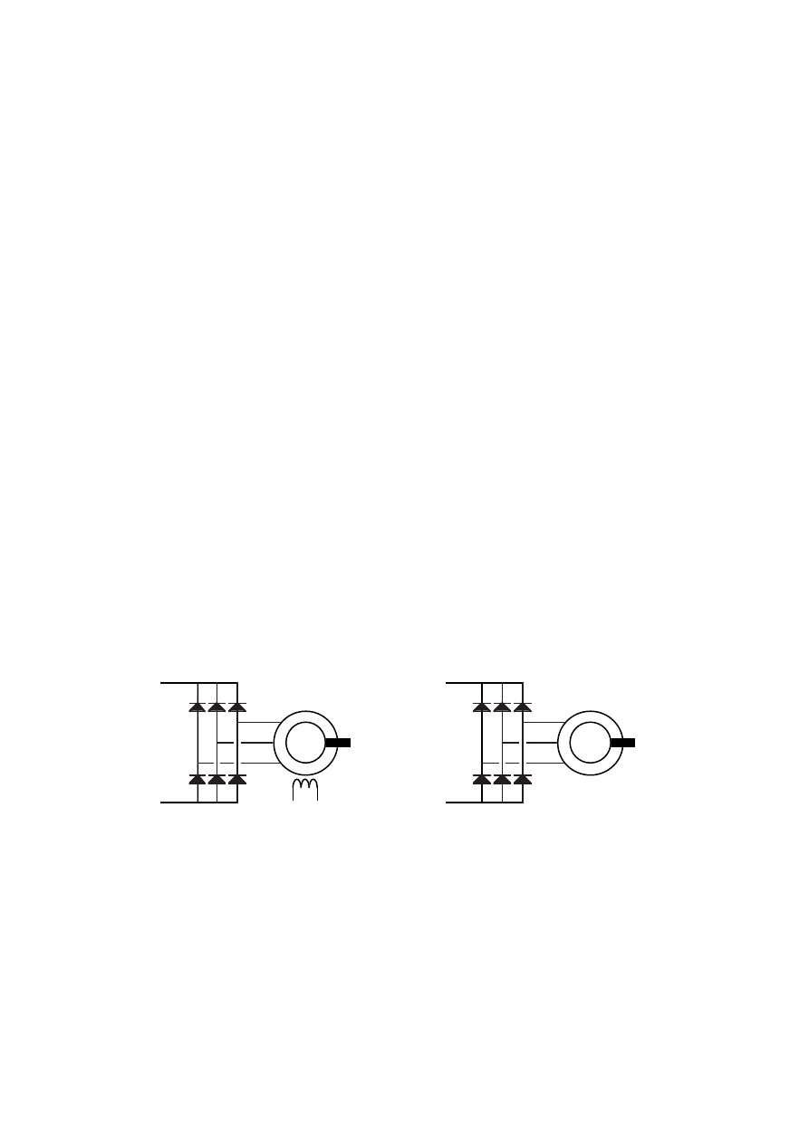
A self commutated inverter can be either a voltage source inverter or a
current source inverter, see Figures 1.4 and 1.5. Today the voltage source
inverter is the most usual type. If it is used to feed power to the network it
must have a constant voltage of the dc capacitor that is higher than the peak
voltage of the network. The generator is not capable of generating a constant
high voltage at low speed and a dc-dc step-up converter must therefore be
used to raise the voltage of the diode rectifier. In a system where the
12
generator is connected to a self-commutated rectifier this is not a problem
since that rectifier directly can produce a high voltage.
SG
400 V network
Voltage source
inverter
570 V
Step-up
converter
0-570 V
Diode
rectifier
0-420 V
Figure 1.4
A variable speed generator system. The frequency converter
consists of a diode rectifier, a step up converter and a voltage
source inverter. The transitors are shown as idealized switches.
SG
Diode
rectifier
0-360 V
400 V network
0-490 V
Current source
inverter
Figure 1.5
A variable speed generator system. The inverter is a current source
inverter with the transistors shown as idealized switches.
For a generator connected to a diode rectifier the self commutated current
source inverter is interesting. It is, like the thyristor inverter, capable of
feeding power to the network from very low voltages. Since the network is a
voltage-stiff system it is from a control point of view good to use a current
source inverter. The drawback of the current source inverter is a lower
efficiency than that of the voltage source inverter with step-up converter.

13
Network-commutated inverters: The usual type of network-commutated
inverter is the thyristor inverter. It is a very efficient, cheap and reliable
inverter. It consumes reactive power and produces a lot of current
harmonics.
Cycloconverters with thyristors are common for large low-speed machines.
They are only used with low frequencies, up to about 20 Hz and therefore
they do not fit the standard four-pole generators used in wind turbine
generator systems. For rotor-cascade connected induction generators the low
frequency range is no disadvantage. The harmonics from the cycloconverter
are large and difficult to filter.
1.2 Wind turbine characteristics
A wind turbine as power source leads to special conditions. The shaft speed-
power function is pre-determined because aerodynamic efficiency of the
turbine depends on the ratio between the blade tip speed and the wind speed,
called tip speed ratio. Maximum aerodynamic efficiency is obtained at a fixed
tip speed ratio. To keep the turbine efficiency at its maximum, the speed of
the turbine should be changed linearly with the wind speed.
The wind power is proportional to the cube of the wind speed. If a turbine
control program that is designed to optimize the energy production is used the
wind speed turbine power function is also a cubic function. The turbine power
curve is shown in Figure 1.7 together with the turbine speed curve. In this
report the turbine speed is assumed to be controllable above the rated wind
speed by blade pitch control. The generator speed can then be considered
nearly constant at wind speeds above the rated wind speed.
An ordinary wind turbine has a rated wind speed of about 13 to 14 m/s but
the median wind speed is much lower, about 5 to 7 m/s. Therefore, the power
of the turbine is most of the time considerably less than the rated power. The
probability density of different wind speeds at the harbour in Falkenberg,
Sweden, is shown in Figure 1.8.
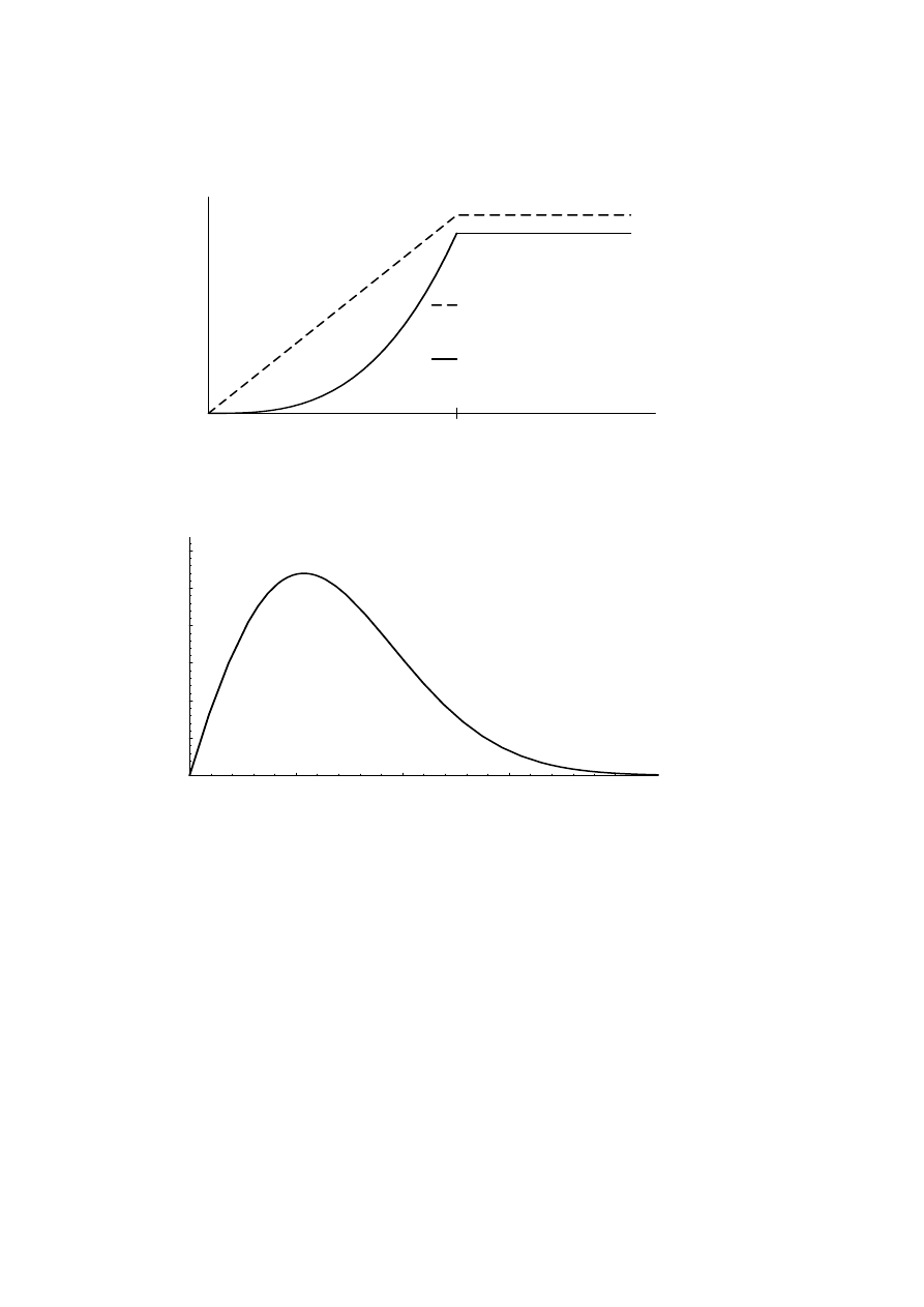
14
Rated wind speed
Wind speed
Speed, Power
Turbine speed
Turbine power
Figure 1.7
The turbine power and turbine speed versus wind speed.
5
10
15
20
Wind speed
(m/s)
0
0.02
0.04
0.06
0.08
0.1
0.12
Weighting function (s/m)
Figure 1.8
The weighting function of wind speeds at the harbour in
Falkenberg, Sweden.
It can be seen that the wind speed usually is about half of the rated wind
speed. Only during a small fraction of the time, less than 10 % of the year, the
turbine produces rated power. Therefore, a generator system for a wind
turbine benefits more of low losses at low power than it does of low losses at
rated power. At high power a variable-speed generator and converter have
higher losses than what a similar generator connected directly to the network
has. However, at low power the variable-speed system can have lower losses
than the network-connected generator. Therefore, the annual average
efficiency can be almost the same for both the systems.

15
1.3 Variable-speed wind turbines
Today most wind turbines run at constant generator speed and thus constant
turbine speed. The reason for this is mainly that grid-connected ac generators
demand a fixed or almost fixed speed. Other reasons may be that resonance
problems are more easily avoided if the speed is constant and that a passive
stall control can be used to limit the power at wind speeds higher than the
rated wind speed.
Reasons for using variable speed instead of fixed speed is that the turbine
efficiency can be increased, which raises the energy production a few percent.
The noise emission at low wind speeds can be reduced. Variable-speed
systems also allow torque control of the generator and therefore the
mechanical stresses in the drive train can be reduced. Resonances in the
turbine and drive train can also be damped and the power output can be kept
smoother. By lowering the mechanical stress the variable-speed system
allows a lighter design of the wind turbine. The economical benefits of this are
very difficult to estimate but they may be rather large.
1.4 A design example system
As an example a system for a 26 meter wind turbine generator system will be
presented in this report. The chosen turbine is a two-blade turbine with a
passive pitch control. Its speed is limited by the pitch control which is
activated by aerodynamical forces. The turbine blade tips will be unpitched
until the turbine speed reaches a pre-set speed, at which the blade tips start
to pitch. The speed will then be kept almost constant with variations of about
±
5 %. This pitch system is completely passive and has no connection with
the power control in the electrical system. The power above rated wind speed
can be kept constant by the generator control. Below rated wind speed the
generator torque will be controlled to keep the optimum tip speed ratio. The
passive pitch system will be inactive and the blades unpitched. At the
optimum tip speed ratio, the turbine can produce 300 kW. The rated wind
speed is then 13 m/s and the turbine speed 72 rpm. 72 rpm is a high speed for
this size of turbine. The speed can be reduced by designing the turbine blades
for a lower optimum tip speed ratio.
16
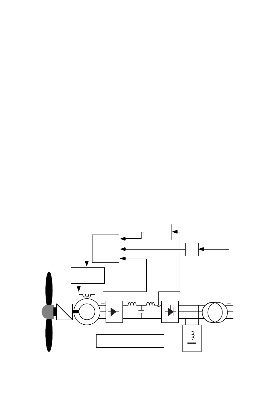
I
a
n
t
n
g
I
E
I
dr
U
d
I
di
I
i
I
net
U
net
U
i
U
a
I
f
P
t
P
g
P
a
P
i
U
di
U
dr
+
+
+
–
–
–
P
d
Figure 2.1
The total system and the quantities used.The generator can be
magnetized either by slip rings or by an integrated exciter.
2 The synchronous generator system
This chapter describes the generator and converter system as well as some
aspects of its design. The component values for the 300 kW design example
system are calculated. Problems are discussed more from an engineers point
of view than from a theoretical point of view.
The complete generator system and its main components are shown in
Figure 2.1. The turbine is described by its power P
t
and speed n
t
. The speed is
raised to the generator speed n
g
via a gear. P
g
is the input power to the
generator shaft. The generator can be magnetized either directly by the field
current I
f
fed from slip rings or by the exciter current I
E
. The exciter is an
integrated brushless exciter with rotating rectifier. The output electrical
power from the generator armature is denoted by P
a
. The generator
armature current I
a
and voltage U
a
are rectified by a three-phase diode
rectifier.
The rectifier creates a dc voltage U
dr
and a dc current I
dr
. On the other side
of the dc filter the inverter controls the inverter dc voltage U
di
and dc current
I
di
. U
d
is the mean dc voltage and I
d
is the mean dc current. The power of the
dc link P
d
is the mean value of the dc power, equal to I
d
U
d
. The inverter ac
current is denoted I
i
and the inverter ac voltage U
i
. The ac power from the
inverter is denoted P
i
.
17
controllable
rectifier
C
U
a lim
Efficiency
control*
Voltage
regulator
U
a ref
*) Efficiency control
or reactive power control
I
di
I
E ref
I
E
U
a
U
net
Figure 2.2
The steady state voltage control of the generator.
The filter is used to take care of the current harmonics by short circuiting the
major part. The output of the generator system is the network current I
net
.
The network voltage is denoted U
net
.
2.1 The control system
The control system of the generator and converter is used to control the
generator torque by current control. In addition to this it can also, by voltage
control with U
a ref
, either control the reactive power consumed by the
inverter or optimize the generator-converter efficiency. The two control
functions are described below.
A voltage control diagram is shown in Figure 2.2. The control of the generator
voltage is achieved by controlling the exciter current by I
E ref
. The control
must be designed to keep the voltage of the generator below about 90 % of
the inverter ac voltage U
a lim
. Otherwise the inverter will not be able to
control the dc-current which will then increase uncontrollably. On the other
hand, the voltage of the generator should not be lower than necessary at
rated power because that leads to a poor power factor of the inverter ac
current. Since the network voltage is not constant these two objectives can
only be reached if the generator voltage is controlled by the measured
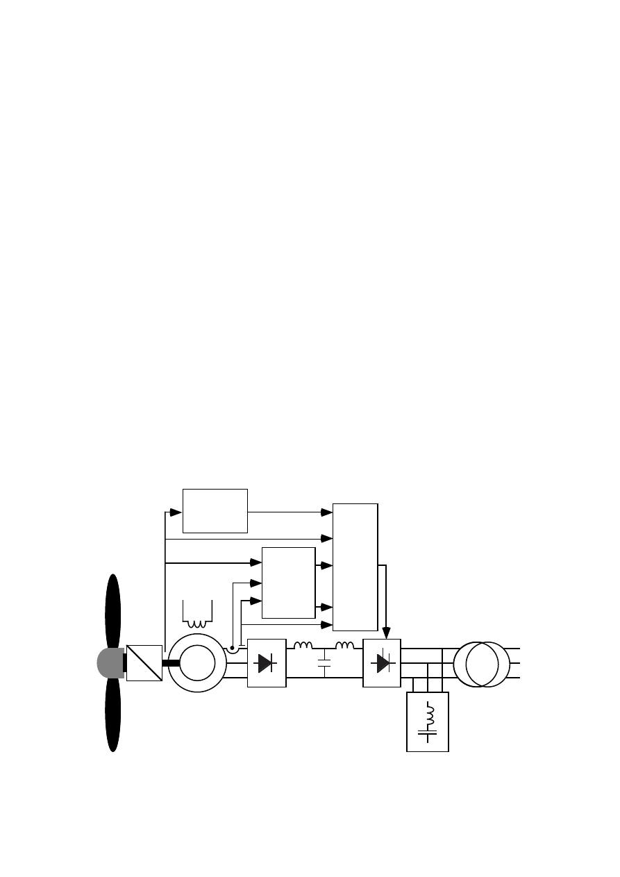
18
T
g ref
Torque
reference
curve
n
g
U
a
Torque
control
I
di ref
I
f
n
g
I
a
n
g
Ψ
Field
current
and
flux link.
estim.
Figure 2.3
The steady state current control and torque control of the
generator.
network voltage. The voltage control must also limit the generator flux. If this
is not done the generator will be saturated which will lead to unacceptable
core losses.
The second item to be controlled is the generator current. It is controlled by
the current reference value to the inverter I
di ref
. At rated power and rated
speed it is kept constant. Below rated power the current is controlled to
obtain a generator shaft torque T
g ref
according to the optimal speed-torque
curve of the turbine. The current demand is calculated from the torque
demand. In Figure 2.3 a diagram for a torque control system is shown.
Because the field current in the rotor and the flux linkage
Ψ
of the stator can
not be directly measured they are estimated from the armature voltage,
armature current and shaft speed.
A fast voltage control is important to keep a high power factor without
commutation problems during voltage dips on the network. If a fast torque
control is required due to, for instance, resonance problems in the drive train,
the two control systems must be designed together. Otherwise they will
disturb each other. Because the current control is obtained by voltage control
of the inverter it is easily disturbed by the voltage control of the generator.
The generator voltage depends on the generator current due to armature
19
reaction and thus the voltage control is easily disturbed by the current
control. One simple solution is to design a fast controller for the generator
voltage and a slower one for the generator current.
2.2 The generator
The generator is assumed to be a standard synchronous generator. Usually it
is a four-pole, 1500 rpm, generator equipped with an integrated exciter and a
rotating rectifier. All the measurements in this report were made on a 50
kVA synchronous generator. It is a Van Kaick generator that is modified by
Myrén & Co AB. The generator, which has an integrated exciter, has also
been equipped with slip rings. This allows magnetization either by the exciter
or by the slip rings. In Figure 2.4 the rating plate of the generator is shown.
2.2.1 Speed rating
In a variable speed system the speed of the generator is not restricted to the
synchronous speed at the network frequency, i.e. 1500 rpm for a 50 Hz
network. Most small generators are designed to operate up to 1800 rpm,
60 Hz, and the only upper limit is their survival speed, 2250 rpm for
Mecc Alte and Leroy Somer generators. Such high speed can, however, not be
used as rated speed. The rated speed must be low enough to allow over-speed
under fault conditions, before the wind turbine emergency brakes are
activated.
FABR
TYP
EFFEKT
VOLT
~
NR
VARV
AMP
MYRÉN & CO AB - GÖTEBORG
GEN
A VAN KAICK
DIB 42/50-4
50 - 60 kVA
360-416 V
MAGN 50 V 27 A
ELLER 40 V 1,1A
SYNKRON
50 - 60
424 118
1500 - 1800
83,5
Figure 2.4
The rating plate of the 50 kVA generator used in the
measurements.
20
-100
-50
0
50
100
0
5
10
15
20
25
30
35
40
Time (ms)
Generator current (A)
Figure 2.5
Armature current wave shape in a generator connected to a
diode rectifier.
The efficiency of a generator is usually increased slightly with increasing
speed. Using high speed also means that a smaller generator can be used to
produce the same power. A generator for 50 Hz operation is 20 % heavier
than a generator for 60 Hz and the same rated power.
A second limitation of the rated speed is the possible gear ratio. Speed ratio
larger than 1:25 between the generator speed and the turbine speed is not
possible for a normal two-stage gear. If higher ratios must be used a three-
stage gear will be necessary. Each extra stage in the gear means 0.5 to 1 %
extra losses. Since the efficiency of the generator only increases some tenths
of a percent there is no reason to use a three-stage gear to reach high
generator speeds. For a two-stage planetary gear the limit of speed ratio is
higher, about 1:50.
2.2.2 Current rating
Harmonics in the armature current make it necessary to reduce the
fundamental current from the rated current to avoid overheating of the
armature windings. The diode rectifier leads to generator currents that are
non-sinusoidal, instead they are more like square-shaped current pulses, see
Figure 2.5. In a standard generator only the fundamental component of the
currents can produce useful torque on the generator shaft. The generator
windings must be rated for the total r.m.s. value of the generator current

21
even if the active power is produced only by the fundamental component. The
armature current of a generator loaded by a diode rectifier has an r.m.s. value
that is about 5 to 7 % higher than the r.m.s. value of its fundamental
component. This means that the generator must have a current rating at
least 5 % higher than what would be necessary if sinusoidal currents were
used.
2.2.3 Voltage rating
An other cause for derating when a diode rectifier is used is the voltage drop in
the commutation inductance. The diode commutation is a short-circuit of two
armature phase windings during the time of the commutation. This short-
circuit leads to a lower rectified voltage compared to the possible voltage if
the commutation was instantaneous. The relative voltage drop due to
commutation can at rated load be approximately determined [6] by the per
unit commutation reactance of the armature windings x
r com
as
∆
U
N
U
N 0
≈
1
2
x
r com
(2.1)
where
∆
U
N
is the commutation voltage drop at rated load and U
N 0
is the
voltage at no load and rated flux.
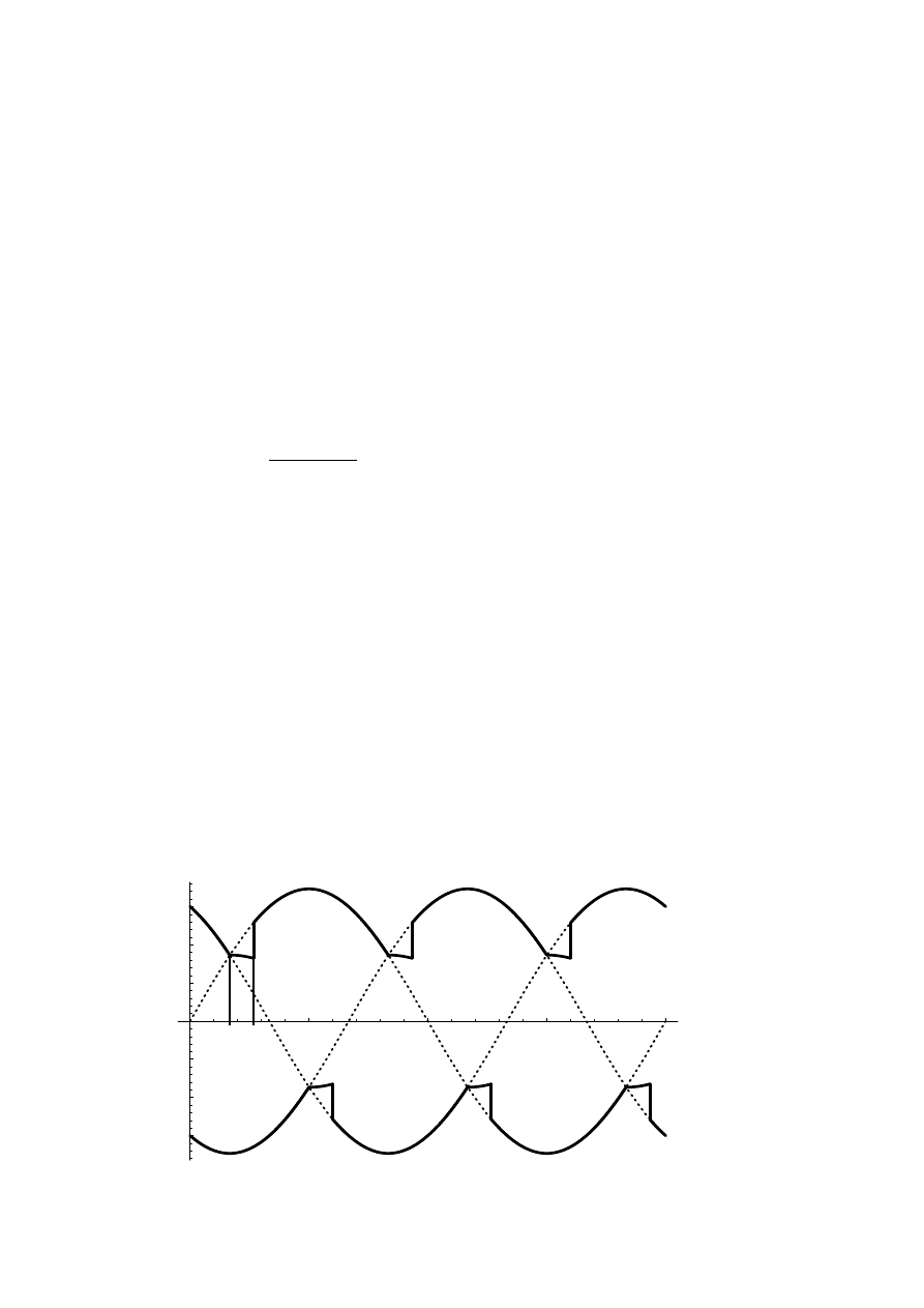
Due to the commutations the voltage of the diode-loaded generator has
commutation notches. They can be seen in Figure 2.6 where the measured
line-to-line voltage of the generator is plotted. An undisturbed wave shape is
also shown for the first half-period. Each half-period has three commutation
notches.
The per unit commutation reactance can be approximately calculated from
the subtransient reactances of the generator [7] as
x
r com
≈
x"
d axis
+ x"
q axis
2
(2.2)
22
-600
-400
-200
0
200
400
600
0
5
10
15
20
25
30
35
40
Time (ms)
Generator volatge (V)
Figure 2.6
Line-to-line armature voltage with commutation notches at
almost rated current. The no load voltage is shown for the first
half-period.
The per unit commutation reactance of standard synchronous generators,
between 200 kVA and 1000 kVA and from two different manufacturers, have
been investigated. The commutation reactance is in the range of 10 % to
26 % with a mean value of about 15 %. The voltage drop of the commutation
is then about 5 to 13 %. If the same generators are used with resistive load
the reduction of armature voltage, when the generator is loaded, is lower. The
voltage drop is then due to the leakage reactance and the armature
resistance. The resistive voltage drop is almost equal for both these cases. It
remains to compare the commutation voltage drop of a diode-loaded
generator with the leakage reactance voltage drop of a resistively loaded
generator. The leakage reactance voltage drop is only a few percent, and
being 90 degree phase-shifted to the armature voltage it does not reduce the
armature voltage significantly. Hence, the equivalent armature voltage for a
diode-loaded generator is about 5 to 13 % lower than for the same generator
resistively loaded.
2.2.4 Other aspects of the rating
With a diode rectifier the harmonics of the armature current induce current
in the damper windings under steady state operation. How large these
currents are and how much losses the damper winding thermally can
withstand has not been included in this study. However, simulations in [4]

23
indicate that they are about 0.2 % at rated current for the 50 kVA generator.
They are not likely to overheat the damper windings and thus these losses
give no reason to derate the generator.
Other additional losses of diode loaded synchronous generators must be
included when the rating is decided. These losses can for example be eddy
current losses in the end region due to the harmonic flux from the end
windings. They make overrating necessary only if they cause overheating of
some part of the generator. The measurements made on the 50 kVA
generator show only about 0.67 % additional losses due to the diode rectifier.
These are such small losses that they probably can be neglected.
2.2.5 Generator rating
The harmonics of the armature current at diode load decrease the
permissible fundamental current about 5 to 7 % compared with a resistively
loaded generator. Due to reactive voltage drop of the commutation
inductance the possible rectified generator voltage is reduced about 5 to 13 %.
Additional losses due to the diode load are small, and they are generally no
reason for derating, if they do not occur in a critical hot spot of the generator.
The generator should have an apparent power rating, for sinusoidal currents,
that is about 10 to 20 % larger than the active power that will be used with
diode load. If the generator is operated at a higher speed than the rated one
the permissible voltage will be raised proportionally to the speed. So, using a
50 Hz machine at 60 Hz increases the voltage rating by 20 %. The limit for
the voltage is set by the isolation of the armature winding. Standard isolation
for 230/400V machines can be used for line-to-line voltages up to 700 V.
The conclusion is that a diode-loaded generator does not need to be bigger
than a generator, for the same active power, connected to a 50 Hz network.
The fundamental component of the armature current has to be lower than
the rated armature current. Also, the possible output voltage is decreased by
the commutations. However, the generator can instead be used with 20 %
higher speed which compensates both for the current and voltage derating at
50 Hz operation.
2.2.6 Generator efficiency

24
When the generator is connected to a diode rectifier the efficiency is lower
than when it is connected to a resistive three-phase load. The reduction does
not only depend on the increase in additional losses, but it is to a large extent
depending on reduced output power at rated current and rated flux. Except for
the additional losses the losses are the same at rated load for the resistive
load as well as for the diode load. The output power is, however, reduced due to
the voltage drop of the commutation and lower fundamental current when a
diode rectifier is used.
At rated current the fundamental of the armature current is about 5 to 7 %
lower with a diode load than with a resistive load. As mentioned earlier the
voltage at rated generator flux is about 5 to 13 % lower with a diode load.
Totally the output power of the generator is 10 to 20 % lower with a diode load
than with a resistive load. Constant losses and lower power reduce the
efficiency. The maximum power of the generator loaded by a diode rectifier P
N
diode
can be expressed as a fraction C
diode
of the maximum power for the
same generator loaded by a three phase resistive load P
N res
P
N diode
= C
diode
P
N res
(2.3)
C
diode
is about 80 to 90 % for the considered generators. The decrease in
rated efficiency due to the derating at diode load,
∆η
N
, is calculated. P
loss N
is
the total generator losses at rated current and rated flux and P
N
is the rated
load. The rated efficiency of generators from 200 kVA to 1000 kVA is about
94 to 96 % at cos(
ϕ
) = 1.0, here the efficiency with resistive load is assumed
to be 95 %. The reduction of efficiency when the generator is loaded by a diode
rectifier instead of a resistive three phase load is
∆η
N
=
η
N res
–
η
N diode
=
1 –
P
loss N
P
N diode
–
1 –
P
loss N
P
N res
=
=
5 %
80 %
–
5 %
100 %
= 1.25 % for C
diode
= 80 %
5 %
90 %
–
5 %
100 %
= 0.56 % for C
diode
= 90 %
(2.4)
The increase in additional losses for the 50 kVA generator when it is
connected to a diode rectifier is

25
∆
P
ad
P
N
≈
0.67 %
(from measurements in Section 3.4.2)
(2.5)
The relative increase in additional losses for generators from 200 to
1000 kVA has not been found. Therefore, the value for the 50 kVA generator
is used instead. The relative increase is probably smaller for the larger
generators because their per unit losses are generally smaller than for the
50 kVA generator.
The total efficiency reduction when a synchronous generator is loaded by a
diode rectifier compared with resistive load is approximately 1.2 to 2.0 %.
About half or more of the decrease in efficiency is because of decreased
output power and not because of increased losses. If the speed of the
generator is higher for the diode-loaded generator compared to the resistively
loaded generator, the difference in efficiency will be a little less.
2.2.7 Design example
The maximum continuous power of the generator system should be 300 kW
at a rated dc voltage of U
d N
= 600 V. This voltage is used because it is the
maximum dc voltage of a standard thyristor inverter and using the maximum
voltage maximizes the efficiency. This means that the rated dc current is I
dr
N
= 500 A. The r.m.s. value of the generator current can be calculated
approximately
I
a
≈
√
2
3
I
dr
= 0.82 I
dr
(2.6)
I
a N
≈
0.82 I
dr N
= 0.82 . 500 A = 410 A
(2.7)
This formula is exact if the dc current is completely smooth. This is not the
case but the increase due to current ripple is only a few percent. Thus the
rated current of the generator should be a little more than 410 A.
According to Ekström [6] the dc voltage can be expressed as a function of the
generator voltage and the dc current
26
U
d
=
3
√
2
π
U
a
–
3
ω
L
r com
π
I
dr
(2.8)
By solving U
a
from this equation and using the rated values of the other
quantities, the rated generator voltage can be found as
U
a N
=
π
3
√
2
U
d N
+
3
ω
N
L
r com
π
I
dr N
(2.9)
An LSA 47.5 generator from Leroy Somer is chosen. The per unit
commutation inductance is 12.6 % at 50 Hz and 410 A which corresponds to
0.226 mH. The generator should, according to Equation (2.9), have a rated
voltage of about 470 V if it is used at 50 Hz and 475 V at 60 Hz.
The voltage can be adjusted not only by choosing generators of different
voltage rating. It can also be adjusted by changing the maximum speed of the
generator. The maximum voltage of a generator is a linear function of speed
U
a max
(n
N
) =
n
n
N
U
a N
(2.10)
For the design example turbine the optimum tip speed ratio
λ
opt
is 7.5 and
the diameter d
t
is 26 m. The rated wind speed v
N
is about 13 m/s. The tip
speed ratio is calculated using the following formula
λ
=
n
t
π
d
t
v
(2.11)
The rated speed of the turbine should then be
n
t N
=
v
N
λ
opt
π
d
t
= 72 rpm
(2.12)
The maximum corresponding generator speed with a gear ratio of 1:25 is
n
g N
= 25 nt
N = 25
.
72 rpm = 1800 rpm
(2.13)
The voltage rating of the generator at 1500 rpm should according to Equation
(2.10) be
27
L
r com
U
a 0
√
3
L
dr
U
d
+
–
I
dr
ω
a
C
d
Figure 2.7
The rectifier circuit including the rectifier reactor L
dr
and the
commutation inductance L
r com
.
U
a N
=
1500 rpm
1800 rpm
475 V = 395 V
(2.14)
Summary:
A generator with at least 410 A current rating and 395 V at
1500 rpm should be used. In other words, a 284 kVA generator (50 Hz) allows
about 300 kW maximum power at 1800 rpm. This is the smallest possible
generator. According to the data sheets of Leroy Somer generators an LSA
47.5 M4 will be sufficient. It can continuously operate with a 290 kVA load at
1500 rpm, 400 V and a class B temperature rise.
2.3 Rectifier
In the rectifier circuit the rectifier reactor L
dr
is also included. The diagram of
the generator and rectifier circuit can be seen in Figure 2.7. The dc voltage U
d
can be considered as a stiff voltage under steady state conditions if the dc
capacitance C
d
is large. U
a0
is the voltage induced by the airgap flux of the
generator and L
r com
is the commutation inductance of the generator
armature.
2.3.1 Diode commutation
The commutation of the dc current between the armature phases of the
synchronous machine is slow because the armature windings have a large
inductance. At rated current the commutation can take up to about 1 ms.
This leads to a lower mean voltage on the dc link at rated load compared with
no load. In Figure 2.8 the potentials of the dc link are shown. A commutation
28
0.005
0.01
0.015
0.02
Time [s]
-600
-400
-200
200
400
600
Potential [V]
t
t
1
2
Figure 2.8
The positive and negative potentials of the dc side of the rectifier.
on the positive side of the diode rectifier takes place between t
1
and t
2
. The dc
potential is during this time equal to the mean value of two phase voltages
instead of the highest phase potential.
2.3.2 Equivalent circuit
The commutation voltage drop can be modelled as a resistance in the dc link
R
r com
. The resistance value depends on the commutation inductance and the
frequency of the ac source. From Equation (2.8) the resistance value can be
identified
R
r com
=
3
ω
L
r com
π
(2.15)
This resistance represents an inductive voltage drop on the ac side and is, of
course, not a source of losses.
The commutation inductance also helps smoothing the dc current. Between
two commutations the dc current passes a series connection of two
commutation inductances, see Figure 2.9. The effective inductance is
between the commutation 2 L
r com
.
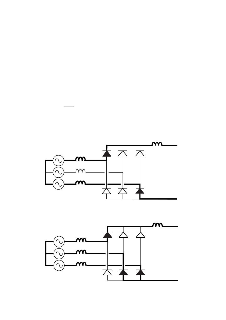
29
U
W
V
Figure 2.9
The current path of the dc current between two commutations.
During a commutation the dc current passes through one commutation
inductance and a parallel connection of two commutation inductances, see
Figure 2.10. The effective inductance is then 1.5 L
r com
.
The commutation inductances will act as a smoothing inductance that is
about twice the per phase commutation inductance of the rectifier.
The no load dc voltage can be calculated from the generator no load voltage
U
dr 0
=
3
√
2
π
U
a 0
(2.16)
The real rectifier circuit can now be replaced in calculations by an equivalent
circuit, Figure 2.11. It includes the effect of the smoothing inductance L
dr
as
U
W
V
Figure 2.10 The current path of the dc current during a commutation from
phase W to V.
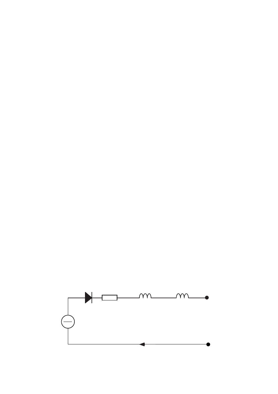
30
U
d
+
–
I
dr
L
dr
2 L
r com
R
r com
U
dr 0
Figure 2.11 The rectifier and generator equivalent circuit at steady state
when the voltage ripple of the rectifier is neglected.
well as the commutation inductance 2 L
r com
. The voltage drop due to the
commutations is modelled as a resistance R
r com
. For a complete model also
the dc resistance and generator armature resistance should be included.
However, the influence of these is small except for the losses of the circuit.
The voltage harmonics are not included in this equivalent circuit.
2.3.3 Design example
In the design example the ratings of the system have been chosen to 300 kW
at a dc voltage of 600 V. Therefore, the diode rectifier should have a rated dc-
current of at least 500 A and a rated dc voltage of 600 V. A diode bridge
consisting of three Semikron SKKD 260 diode modules and a isolated heat
sink is chosen. With appropriate cooling this rectifier can continuously
operate at a dc current of 655 A.
The isolated heat sink is advantageous because the power circuit in a wind
turbine generator system should not be exposed to the ambient air. The heat
sink must, however, be cooled by ambient air since the dissipated power is
high, about 1.5 kW at rated power. This can be solved by using an isolated
heat sink which is earth-connected and is a part of the enclosure for the
power circuit. The cooling fan is placed outside the enclosure while all the
wiring as well as the diode modules are inside.
The voltage drop of each diode in a SKKD 260 module is 1 V, independent of
the load, plus the voltage drop of 0.4 m
Ω
resistance. The total losses of the
diodes in the rectifier can be expressed as
P
loss r
= 2 V I
d
+ 0.8 m
Ω
(I
d
)
2
(2.17)

31
Expressed in per unit of the rectifier rated current and rated power the losses
are
p
loss r
= 0.33 % i
d
+ 0.07 % (i
d
)
2
(2.18)
Also some resistance in the connections and the cables should be included in
the losses leading to a higher resistive loss. The total rectifier losses can then
be expressed as
p
loss r
= 0.33 % i
d
+ 0.17 % (i
d
)
2
(2.19)
2.4 Dc filter
In this section the dc harmonics will be described as well as some aspects of
the design of the dc filter.
The dc-filter is used for four purposes:
(1) It is supposed to prevent harmonics from the rectifier to reach the
network. If there are harmonics from the rectifier in the network current
they can not be easily filtered since their frequency changes with the
generator speed. They can also cause resonance in the filter for the inverter
harmonics because it has resonance frequencies below the frequencies of the
characteristic harmonics.
(2) The dc filter should also keep the harmonics from the inverter low in the
rectifier dc current, since they would otherwise cause power oscillations and
generator torque oscillations. For generator frequencies close to the network
frequency these oscillations have low frequency and then they can cause
mechanical resonance.
(3) The harmonic content of the generator current depends to some extent on
the dc filter. The filter should be designed to keep the harmonic content low
because the harmonics cause extra losses in the generator.
(4) The dc filter design also affects the amount of harmonics produced by the
inverter. The fourth purpose of the dc filter design is to assure that the
inverter ac current harmonics are low and easy to filter.
32
L
d
C
d
L
di
L
dr
C
d
L
di
L
dr
L
d C
type A
type C
type B
Figure 2.12 The investigated dc filter types.
If the dc filter consists of both inductances and capacitances it has
resonance frequencies. They must not be excited by any of the larger
harmonics that may occur during normal operation. Dc link harmonics
occurring only under fault conditions can be allowed to be amplified by the
resonances, if the converter is disconnected before the resonance has caused
any damage. Since the generator fundamental frequency has a wide range,
the filter resonance probably has to be damped because it is practically
impossible to avoid all the harmonic frequencies.
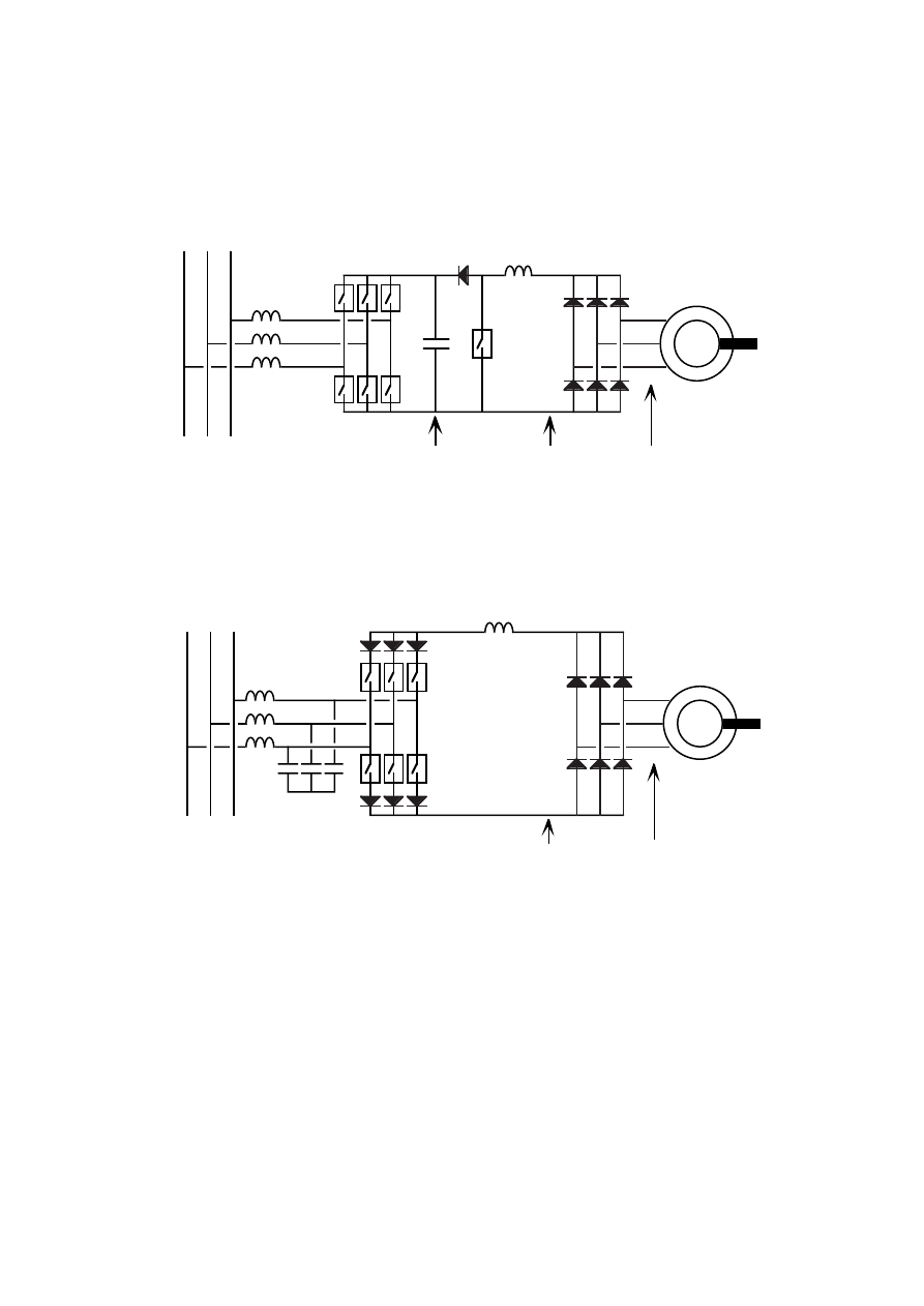
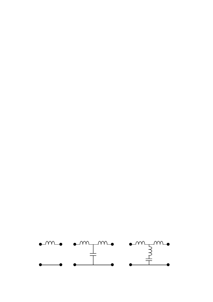
2.4.1 Filter types
Three simple types of dc-filters have been investigated and they are shown in
Figure 2.12. The simplest filter possible, type A, has only one inductance. All
the current harmonics generated by the rectifier will appear as inter
harmonics in the inverter current. To reduce these inter harmonics L
d
has to
be large. This is expensive and leads to a slow current control and therefore
slow torque control.
A short circuit link can be used to make the dc filter more effective in
reducing the inter harmonics in the inverter current. The second filter type B
is a filter with a capacitance between two dc reactors. The capacitance will
short-circuit most of the harmonics and it adds almost no extra losses. By
stabilizing the voltage it separates the problem of current smoothing into two
parts. The network side dc-current is smoothened by L
di
and the generator
side dc-current is smoothened by L
dr
. The capacitance must be large enough
to filter the low rectifier harmonics well.
The third filter type C is a variant of the type B filter. An inductance is
introduced in the short-circuit link and the link is tuned to more effectively
33
0
200
400
600
800
1000
Freq. (Hz)
0.001
0.01
0.1
1
10.
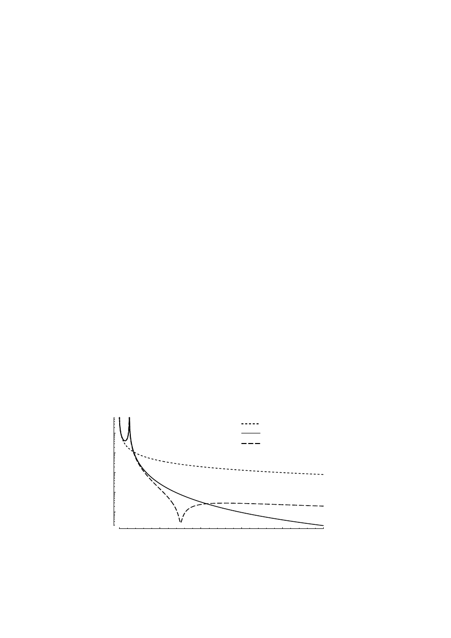
Filter gain (A/V)
A type
B type
C type
I / U
di
dr
(A/V)
Figure 2.13 The inverter harmonic current relative to the rectifier harmonic
voltage, I
di
/ U
dr
.
short-circuit the largest fixed frequency harmonic. Only the harmonics from
the inverter have constant frequencies. The largest harmonic from the
inverter is the 300 Hz harmonic. But even without L
d C
the 300 Hz current is
damped very well and the higher harmonics are reduced better without L
d C
.
The harmonic current in the inverter dc current relative to the rectifier
harmonic voltage, I
di
/ U
dr
, for the three types of dc filter is shown in Figure
2.13. The choice of dc filter will probably be between type A and type B. The
filter of type B has much better damping of the harmonics. The single
inductance L
d
in filter A is higher than L
di
plus L
dr
in filter B. On the other
hand, filter B is more complicated, has more parts and it probably has to
have a circuit to damp its resonance. Non-characteristic harmonics in the
inverter current can cause resonance in the ac filter. These harmonics can be
reduced much better by filter B than by filter A. Therefore, a filter of type B
is chosen for this design example, but this choice is not based on a complete
study of all the important aspects.
2.4.2 Harmonics in the dc link
The harmonics in the dc link are originating from the frequencies of the
network and the generator. The thyristor inverter and the diode rectifier
generate a dc voltage with a superimposed ac voltage. Under ideal conditions
the harmonic frequencies of the dc voltages are integer multiples of six times

34
the ac frequencies. Only the sixth and twelfth harmonics cause ripple
currents of considerable magnitude. From the inverter side a 300 Hz and a
600 Hz current are generated. Depending on the generator frequency, from
25 to 60 Hz, the diode rectifier generates a current harmonic with a
frequency between 150 Hz and 360 Hz. The twelfth harmonic generated by
the diode rectifier has a frequency between 300 Hz and 720 Hz. The
magnitude of these voltage harmonics are depending on the generator voltage
and on the firing angle of the inverter.
Under non-ideal conditions also other harmonics occur. If, for instance, the
network voltage or the generator voltage is unsymmetrical, a second
harmonic will also be generated. This should under normal conditions be
small, but must not be amplified by resonance in the dc filter. Non-ideal firing
of the inverter thyristors also causes other harmonics. They can be of any
multiple of the fundamental frequency, but should for well-designed firing
control systems be small. In Figure 2.14 the harmonics from the inverter and
rectifier are illustrated.
A reason for unusual harmonics in the dc link is fault conditions. These
harmonics must of course not damage the converter and therefore their
effect must be calculated. If one ac phase is disconnected, because of for
instance a blown fuse, a very large second harmonic is generated. The three-
phase rectifier will then start to act as a one phase rectifier.
If a diode or a thyristor valve is short-circuited due to a component failure, a
current of the fundamental frequency is generated in the dc link. The result
should be that a fuse is blown.
All the above mentioned voltage harmonics can cause high currents if their
frequencies are close to the dc link resonance frequencies. Therefore, the dc
link resonance frequencies have to be carefully chosen. It is clear that the
resonance frequencies have to be below 150 Hz due to rectifier harmonics.
The second harmonic of both the network frequency and the generator
frequency must also be avoided, if the resonance is not well damped. Very low
resonance frequencies should also be avoided because they lead to a slow step
response of the current control. In the design example a filter with a rectifier
side resonance at 75 Hz is suggested.
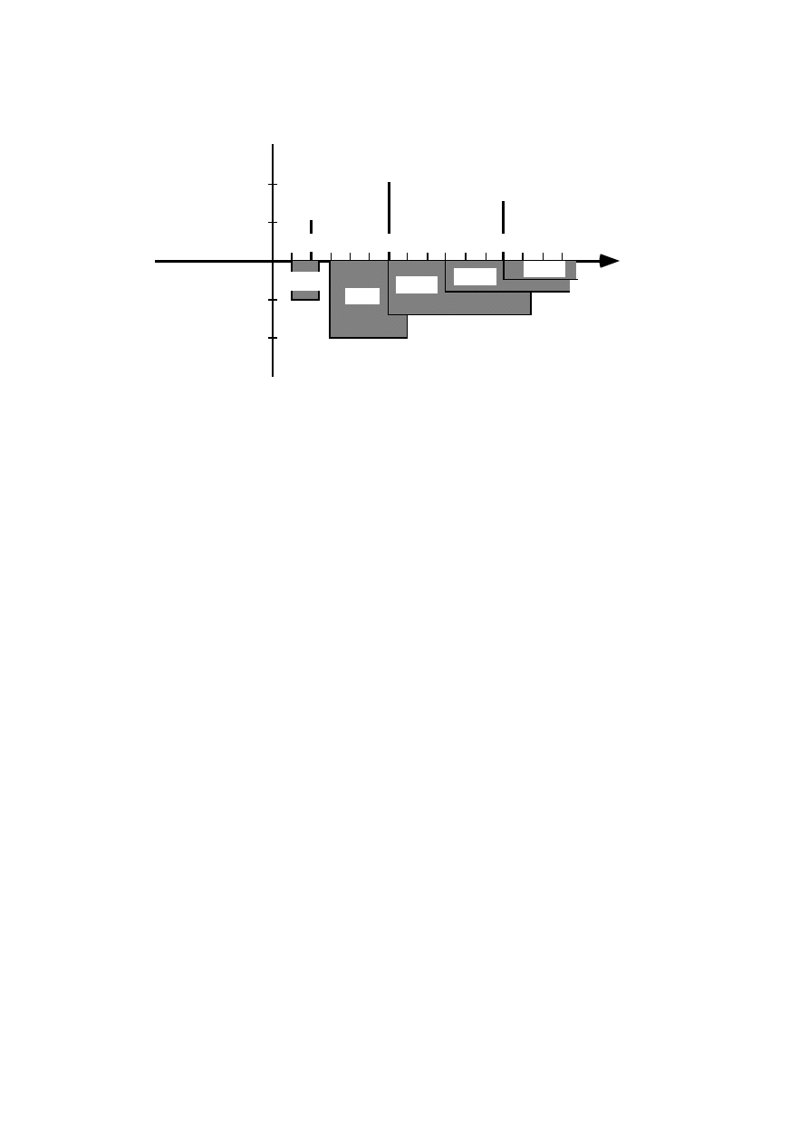
35
Harmonics from
the rectifier
2:nd
6:th
12:th
600
300
frequency
(Hz)
100
small
small
large
large
2:nd
18:th
6:th
12:th
Harmonics from
the inverter
24:th
Figure 2.14 The harmonic frequencies in the dc filter under normal
conditions and symmetrical firing.
2.4.3 Smoothing reactor of the diode rectifier
The current harmonics of the rectifier dc current depend on the magnitude of
the harmonic voltages from the rectifier and on the smoothing inductance.
For economical reasons the inductance should be minimized. The maximum
acceptable ripple in the dc current must, therefore, be determined. On the
generator side, the rectifier-induced harmonics are interesting mainly
because they cause losses in the generator. Higher ripple means higher r.m.s.
current and makes it necessary to use a higher current rating of the
armature winding.
The harmonics from the inverter are small if a filter of type B or C is used.
They do not have to be considered when the size of L
dr
is calculated.
The r.m.s. value of the generator current can be calculated for different ripple
magnitudes. This is done assuming a ripple-free dc voltage U
d
over the dc
filter capacitor and instantaneous commutations. The r.m.s. value as well as
the fundamental component of the generator current are calculated. In
Figure 2.15 the relation between the r.m.s. value and the fundamental of the
armature current are plotted. For a perfectly smoothed dc current the r.m.s.
value of the generator armature current is 4.7 % higher than its fundamental
component. When the ripple increase the r.m.s. value of the generator
current increases slowly. At a peak-to-peak ripple of 20 % of the rated dc
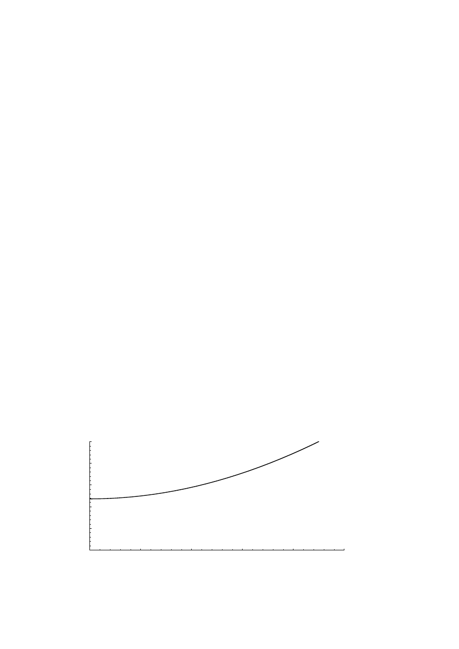
36
0.2
0.4
0.6
0.8
1
Ripple
(p.u.)
1
1.02
1.04
1.06
1.08
1.1
I-a/I-a(1)
I / I
a
a(1)
Figure 2.15 The r.m.s. value of the generator current relative to the
fundamental component versus the relative peak-to-peak ripple.
current the armature current r.m.s. value is about 5 % higher than the
fundamental component. At a 60 % ripple the r.m.s. value of the armature
current is 7 % higher than the fundamental.
The increase in the r.m.s. current will be small, if the ripple is less than 60 %
of the dc current mean value. As the peak-to-peak ripple increases from
20 % to 60 % the r.m.s. value of the current only increases from 1.05 to 1.07
times the fundamental component. The r.m.s. current only increases about
2 % while the ripple increases three times. Three times higher ripple allows a
three times smaller total smoothing inductance. A 2 % increase in armature
current increases the copper losses of the generator by about 4 %. At the
same time the dc link losses should decrease as least as much since the
smoothing inductance is decreased to a third.
A complete design study may show that other restrictions than generator
losses determine the value of the smoothing inductance. The resonance
frequencies must be kept at certain frequencies and a high ripple leads to a
high peak value of the dc current. The peak value of the current determines
the size of the iron core of the dc reactor. Therefore, higher peak current
means a more expensive reactor.
The first step in determining the rectifier smoothing inductance is to chose
the maximum allowed peak-to-peak ripple at rated current. Then the
neccesary inductance can be calculated. The ac current through the rectifier
37
t3
t4
I-dr
U-dr
U-d
I
U
U
dr
d
dr
3
4
t
t
Figure 2.16 The rectifier dc voltage U
dr
, dc capacitor voltage U
d
and the
rectifier dc current I
dr
. The integration interval to find the peak-
to-peak value is from t
3
to t
4
.
dc reactor L
dr
can under stationary conditions be found by integrating the
voltage over the total smoothing inductance. The voltage over the dc filter
capacitance is assumed to be a perfectly smooth dc voltage. The ac
component of the rectifier dc current is calculated as
I
dr
(t) =
⌡
⌠
1
L
tot
(
)
U
dr
(t) – U
d
dt (2.20)
To find the peak-to-peak ripple the integral (2.20) is evaluated from t
3
to t
4
.
The integration interval is the part of the voltage ripple period where the
voltage over the smoothing inductance is positive. The voltage on both sides
of the inductance as well as the dc current can be seen in Figure 2.16.
The relation between peak-to-peak ripple, generator voltage and total
smoothing inductance can now be calculated for the rectifier as
∆
I
dr p-p
=
⌡
⌠
t
3
t
4
√
2 U
a
L
tot
sin(
ω
t +
π
3
) –
3
π
dt (2.21)
where
L
tot
= L
dr
+ 2 L
r com
t
3
: when the voltage over the inductance becomes positive
t
4
: the voltage over the inductance becomes negative again
U
a
is the no-load armature voltage

38
Both t
3
and t
4
are found as solutions for t in the equation
sin(
ω
t +
π
3
) =
3
π
(2.22)
for which
0 <
ω
t
3
<
π
6
and
π
6
<
ω
t
4
<
π
3
2.4.4 Smoothing reactor of the inverter
The total r.m.s. value of the network ac current is also depending on the dc
reactor L
di
just as for the rectifier. However, there are other aspects that are
more important for the inverter current than just minimizing the total r.m.s.
value. The ac harmonics of the inverter current are very important to
evaluate. They must be below certain limits to be accepted by the utility. If
the dc current is assumed perfectly smooth it can be shown that the current
harmonics are inversely proportional to their frequencies as described by the
formula
I
i (k)
=
I
i (1)
k
(2.23)
where k is the order of the harmonic.
If the ripple on the dc current increases most of the ac harmonics will
decrease. Only the fifth current harmonic increases with higher dc current
ripple, see Figure 2.17. The magnitude of the harmonics is calculated
assuming a ripple-free dc voltage U
d
, no overlap of the inverter ac currents
and a second order approximation of the ripple current wave shape.
The increase of the fifth harmonic is, of course, important since it is the
largest current harmonic. However, being that large also makes it the one
that is almost always necessary to filter. If a good harmonic filter already is
installed for the fifth harmonic, the effect of increasing it can be rather small.
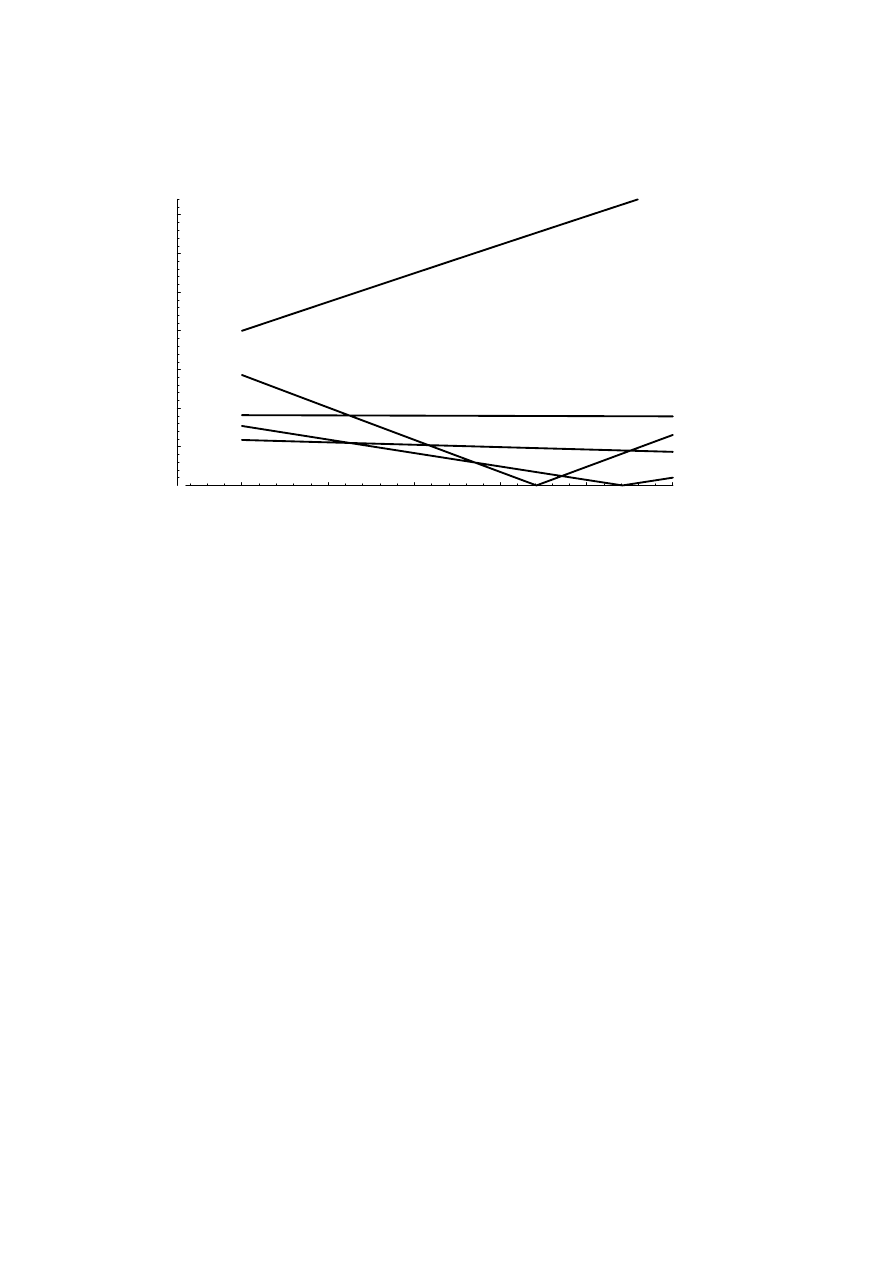
39
0
0.2
0.4
0.6
0.8
1
Ripple
(p.u.)
0.05
0.1
0.15
0.2
0.25
0.3
0.35
I-i(k)/I-i(1))
k=5
k=7
k=11
k=13
k=17
I / I
i(k)
i(1)
Figure 2.17 The ac current harmonics at rated power relative to the
fundamental current at different dc current peak-to-peak ripple.
No overlap and a second order approximation of the ripple
current wave shape is assumed.
The seventh, thirteenth and nineteenth current harmonics etc. are decreased
significantly by the ripple. The most interesting of these harmonics is the
seventh one because it is often necessary to filter. If it can be reduced
significantly, the seventh harmonic filter link may be unnecessary.
The eleventh, seventeenth and twentythird harmonics etc. are not reduced as
much as the others. Therefore, they have to be filtered. This can be done by
means of a filter link for the eleventh harmonic with a high pass
characteristic.
As can be seen in Figure 2.18 the seventh harmonic is low at high power but
will increase when the power is reduced below 0.6 p.u. It is, therefore, not
sufficient only to make sure that the magnitude of the seventh harmonic is
low at rated power; it is not allowed to increase too much at lower power
either. A seventh harmonic that is higher at low power than at rated power
can, however, be acceptable if most of the other harmonics then are lower.
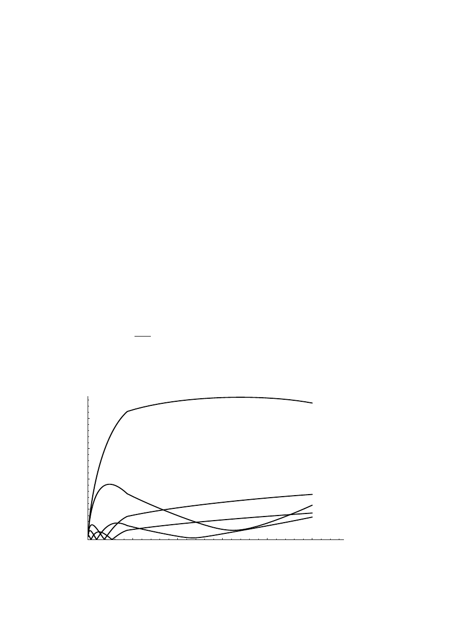
40
0.2
0.4
0.6
0.8
1
P-d
(p.u.)
0
0.05
0.1
0.15
0.2
I-i(k) (p.u.)
k=5
k=11
k=7
k=17
k=13
i(k)
(p.u.)
d
(p.u.)
I
P
Figure 2.18 The magnitude of the current harmonics as a function of power.
At rated power the dc current ripple is 35 % peak-to-peak. The
harmonics are calculated from a wave shape including the effect
of changing fire angle but not including overlap.
There is, of course, a drawback of reducing ac harmonics by increasing the dc
current ripple. The peak value of the inverter dc current then increases,
demanding a higher current rating of the dc reactor.
No clear rules for choosing the inverter inductance can be given here. An
interesting prospect, however, is to have a large current ripple of the dc
current at rated current, approximately a peak-to-peak ripple in the order of
35 % of the mean current. By doing so, it ought to be possible to design an
appropriate ac filter with only two LC-links.
The first step in determining the inverter smoothing inductance is to chose
the maximum allowed peak-to-peak ripple at rated current. When it has been
decided the smoothing inductance can be calculated. Under stationary
conditions the ac current through the inverter dc reactor L
di
can be found by
integrating the voltage over the total smoothing inductance. The ac
component of the inverter current I
di
can be calculated from the inverter
voltage U
di
and the dc voltage U
d
as
I
di
(t) =
⌡
⌠
1
L
tot
(
)
U
di
(t) – U
d
dt (2.24)
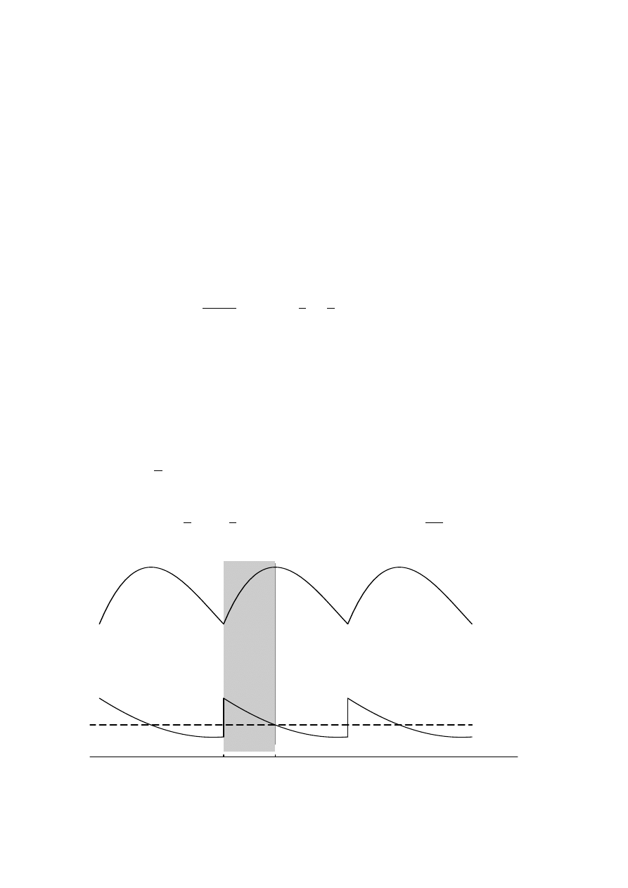
41
t1
t2
I-di
U-di
U-d
I
U
U
t t
di
d
di
5
6
Figure 2.19 The inverter dc voltage U
di
, dc capacitor voltage U
d
and the
inverter dc current I
di
. The integration interval to find the peak-
to-peak value is from t
5
to t
6
.
To find the peak-to-peak value of the ripple, the integral is evaluated with a
lower limit t
5
and an upper limit t
6
. The integration interval is equal to the
part of the voltage ripple period where the voltage over the smoothing
inductance is positive. The voltage on booth sides of the inductance as well as
the dc current can be seen in Figure 2.19. The firing angle is 150˚.
Now the relation between peak-to-peak ripple, ac voltage, smoothing
inductance and firing angle can be expressed as
∆
I
di p-p
=
⌡
⌠
t
5
t
6
√
2 U
i
L
tot
sin(
ω
t +
π
3
) +
3
π
cos(
α
) dt (2.25)
where
L
tot
= L
di
+ 2 L
i com
U
i
is the inverter ac voltage
t
5
: the firing time of a thyristor
t
6
: the time the voltage over the inductance becomes negative
The time instants t
5
and t
6
are determined by the following equations
t
5
=
α
ω
(2.26)
sin(
ω
t
6
+
π
3
) = –
3
π
cos(
α
N
)
and
α
<
ω
t
6
<
4
π
3
(2.27)

42
For a thyristor inverter the firing angle
α
is about 150˚ to 155˚ at rated
voltage.
2.4.5 Dc capacitance
When L
dr
and L
di
have been chosen the capacitance C
d
can be calculated. It
is determined by the desired resonance frequency
C
d
=
1
(L
dr
+ 2 L
r com
) ( 2
π
f
r
)
2
(2.28)
where f
r
is the chosen resonance frequency for the rectifier side harmonics.
If C
d
is very large the values of the inductances already calculated can of
course be increased. An important reason to keep them small is, however,
their resistive losses. The losses must be included in such a trade-off between
capacitance and inductance.
2.4.6 Resonance damping
The resonance of the dc filter can be damped by means of an RLC circuit
tuned to the resonance frequency, see Figure 2.20. If only one damping circuit
should be used and both the rectifier side and the inverter side resonance
frequencies must be damped, the dc filter including the commutation
inductances, must be symmetrical. In this way the two resonance
frequencies become equal because the total smoothing inductance on both
sides are equal
L
di
+ 2 L
i com
= L
dr
+ 2 L
r com
(2.29)
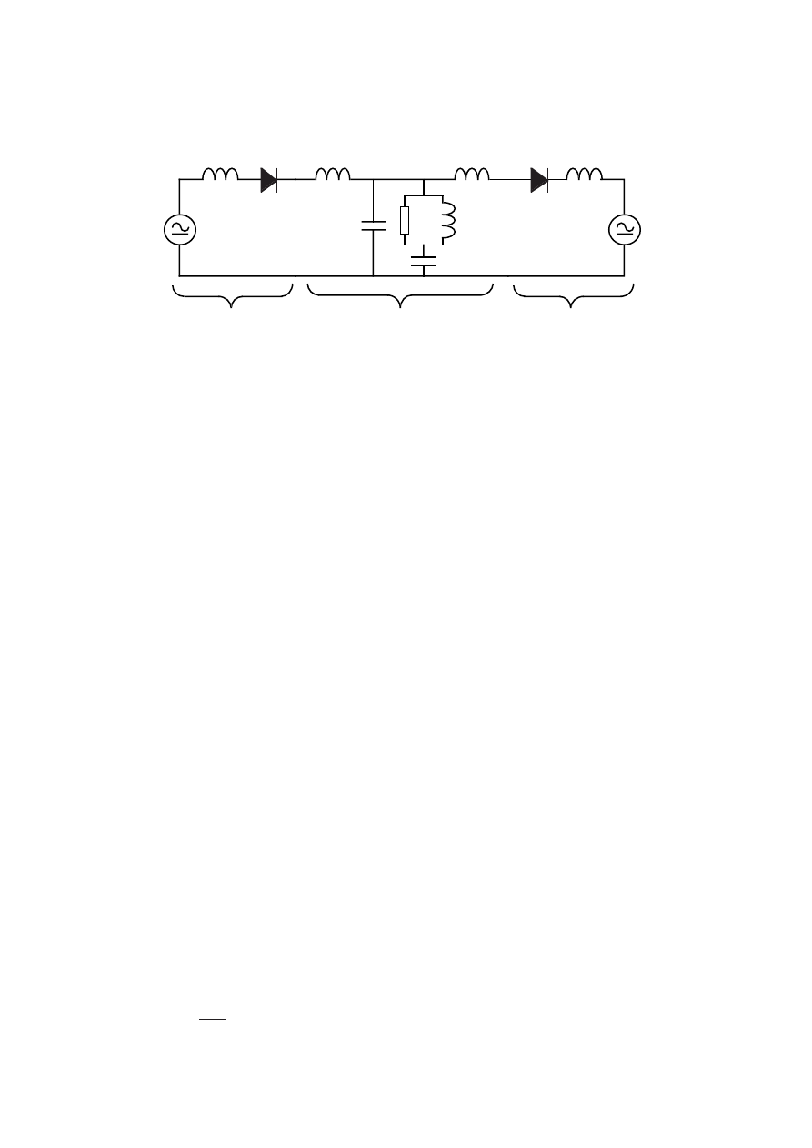
43
C
x
L
di
L
dr
L
x
R
x
C
d
2 L
i com
2 L
r com
U
di
U
dr
Rectifier model
Inverter model
Dc filter with damping
Figure 2.20 The dc filter with damping circuit, rectifier and inverter model.
The the effect of the damping circuit on the transfer function of the dc filter is
shown in Figure 2.21. For high harmonics (>100 Hz) the damping circuit can
be neglected and considered as an open circuit.
2.4.7 Dc filter calculations for the design example system
The design example generator and converter system has the following data:
Ac voltage of the inverter
U
i N
= 500 V
Network angular frequency
ω
i
=
2
π
50 rad/s
Inverter commutation reactance
x
i com
= 5 %
Firing angle at rated load
α
N
= 155˚
Rated dc current
I
d N
= 500 A
Rated generator voltage
U
a N
= 475 V
Rated generator angular frequency
ω
g N
= 2
π
60 rad/s
Rect. commutation reactance
x
r com
= 12.6 %
Network per unit base impedance
Z
b net
= 0.69
Ω
Generator per unit base impedance
Z
b g
= 0.67
Ω
The damping circuit is not included in this design.
The peak-to-peak ripple of the inverter side dc current I
di
at rated power is
chosen to 35 % of the rated dc current. Then the value of L
di
can be
calculated from Equations (2.25), (2.26) and (2.27)
t
5
=
α
N
ω
i
= 8.61 ms
(2.30)
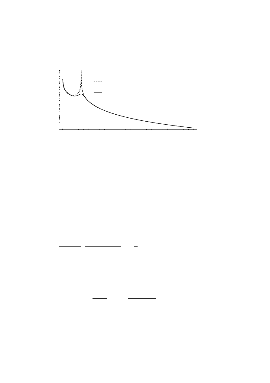
44
0
100
200
300
400
500
Freqency
(Hz)
0.01
0.1
1
10.
100.
1000.
Filter gain (A/V)
Without damping
With damping
I / U
di
dr
(A/V)
Frequency
(Hz)
Figure 2.21 The transfer function of the dc filter with and without damping.
sin(
ω
i
t
6
+
π
3
) =
3
π
cos(
α
N
)
and
α
<
ω
i
t
6
<
4
π
3
⇒
⇒
t
6
= 10.0 ms
(2.31)
L
di
+ 2 L
i com
=
√
2 U
i N
0.35 I
d N
⌡
⌠
t
5
t
6
sin(
ω
i
t +
π
3
) +
3
π
cos(
α
N
) dt =
=
√
2 U
i N
0.35 I
d N
–cos(
ω
i
t +
π
3
)
ω
i
+ t
3
π
cos(
α
N
)
t
6
t
5
= 0.75 mH
(2.32)
The inverter commutation inductance is the transformer leakage inductance
plus a small contribution from the network reactance that can be neglected
L
i com
= x
i com
Z
b net
ω
i
= 0.05
0.69
Ω
100
π
rad/s
= 0.1 mH
(2.33)
This makes the dc filter inductance
L
di
= 0.55 mH
(2.34)

45
The rated dc current is 500 A. The ripple current peak value is 0.5
.
35 %
times the rated dc current. That makes the peak value of the dc current
I
di
^
≈
1 +
0.35
2
I
di
_
= 590 A
(2.35)
The r.m.s. value of the rated current is approximately
I
di
≈
I
di
_
= 500 A
(2.36)
The inverter side smoothing reactor should have a core large enough for 590
A peak current, but the inductor winding needs only be rated for about 500 A
r.m.s. value, and the inductance should be 0.55 mH.
The rectifier side smoothing inductance is calculated using Equations (2.21)
and (2.22)
sin(
ω
g N
t
x
+
π
3
) =
3
π
⇒
ω
g N
t
x
=
0.222
±
n 2
π
0.825
±
n 2
π
rad
(2.37)
0 <
ω
g N
t
3
<
π
6
⇒
t
3
= 0.59 ms
(2.38)
π
6
<
ω
g N
t
4
<
π
3
⇒
t
4
= 2.19 ms
(2.39)
L
dr
+ 2 L
r com
=
√
2 U
a N
∆
I
dr p-p
⌡
⌠
t
3
t
4
sin(
ω
g N
t +
π
3
) –
3
π
dt =
=
√
2 U
a N
0.35 I
d N
–cos(
ω
g N
t +
π
3
)
ω
g N
+ t
3
π
t
4
t
3
= 0.18 mH
(2.40)
The commutation inductance of the generator is 12.6%
L
r com
= x
r com
Z
b g
ω
g N
= 0.126
0.67
Ω
60 2
π
rad/s
= 0.224 mH
(2.41)

46
which makes the rectifier dc inductance unnecessary.
L
dr
= 0 mH
(2.42)
Even without the rectifier inductance the ripple of the rectifier dc current will
only be about 70 A.
The dc capacitance is determined by the chosen resonance frequency. In this
example the rectifier side resonance frequency is chosen to be 75 Hz. From
Equation (2.28) the dc capacitance can be calculated
C
d
=
1
(L
dr
+ 2 L
r com
) ( 2
π
f
r
)
2
= 10 000
µ
F
(2.43)
The filter has now two resonance frequencies. The rectifier side resonance
frequency is 75 Hz and the inverter side resonance frequency is
f
i
=
1
2
π
√
(L
di
+ 2 L
i com
) C
d
= 58 Hz
(2.44)
If both resonances must be damped with one damping circuit the rectifier
should be equipped with a reactor to make the resonance frequency equal on
both sides. In that case
L
dr
= L
di
+ 2 L
i com
– 2 L
r com
= 0.3 mH
(2.45)
The losses of the dc filter have not been calculated exactly, but they are
estimated to be 0.7 % at rated load.
2.5 Inverter
Major reasons to choose the line-commutated thyristor inverter are the high
efficiency, about 99 %, and the low price compared with other inverter types.
Disadvantages are that it generates harmonic currents and consumes
reactive power. The thyristor inverter is also difficult to protect at network
faults.
47
Y:Y
Y:
∆
≈
5%
≈
5%
<2%
~
To
consumers
Filter
≈
5%
<2%
~
Filter
Transf.
leakage
reactance
Transf.
leakage
reactance
(a)
(b)
Figure 2.22 (a) Twelve-pulse and (b) six-pulse connected inverter. Equivalent
single line scheme including the transformer leakage reactance
and network short-circuit reactance.
2.5.1 Inverter pulse number
Large thyristor inverters are often made of two six-pulse bridges in a twelve-
pulse connection to reduce the current harmonics. The twelve-pulse
connection eliminates every second of the characteristic harmonics
generated from a six-pulse inverter. This is done by connecting the two six-
pulse inverters in series on the dc side, see Figure 2.22. On the ac side they
are connected to two phase-shifted three-phase systems created by a three-
winding transformer.
The drawbacks of the twelve-pulse connection for a medium size wind turbine
generator system are both technical and economical.
The first technical drawback is that if the reactive power must be
compensated, the network harmonic filters for the twelve-pulse connection
will not be smaller than the ones used for a six-pulse bridge. The size of the
filter is determined by the reactive power consumed by the inverter and the
twelve-pulse inverter consumes as much reactive power as the six-pulse
inverter.
In the twelve-pulse connection the filtering must be made on either both low
voltage three-phase systems or on the high-voltage side of the transformer.
Both these alternatives complicate the design and the manufacturing. A

48
filter connected to the 10 kV network can not easily be integrated with the
windmill electrical system. If the filter of the twelve-pulse inverter is
connected to the network side of the transformer it does not benefit of the
leakage inductance of the transformer which makes a filter on the low
voltage side several times more effective. In Figure 2.22 it can be seen that
the harmonic voltages of the network, for the six-pulse connection, are only a
fraction of the harmonic voltages of the filter. The harmonic voltages are
reduced because the voltage of the filter is divided by the network impedance
and the transformer impedance. In this example the harmonic voltages of the
filter are reduced at least to 2/7. For the twelve-pulse connection the
harmonic voltages of the filter are instead the same as those of the network.
The filter impedance must be lower in the twelve-pulse connection than in the
six pulse connection to reduce the network harmonic voltages to an equally
low level.
It is also easier to calculate the filtering effect and the resonance frequency if
the filter is connected to the low voltage side of the transformer. The
transformer reactance can for low harmonics be assumed to be substantially
larger than the network impedance. Therefore, the usually unknown
variations in the network impedance do not change the effect of the filter
much. A filter connected directly to the network must also be designed to
filter harmonics from other sources otherwise it might be overloaded. The
filter connected on the low-voltage side of the transformer might also be
burdened with harmonics from the network but to a much smaller extent.
The economical drawbacks of the twelve-pulse connection are a more
expensive transformer and converter. The transformer is more expensive due
to the doubled secondary windings. For small converters, less than about 1
MW, the six-pulse inverter is a standard equipment. It is cheaper to buy a
large six-pulse inverter than to use two smaller inverters in a twelve-pulse
connection.
A twelve-pulse connection is, for several reasons, not likely to be used in
small systems, at least not in systems less than 1 MW. The transformer and
the converter are more expensive. Even though every second of the
harmonics are eliminated by the twelve-pulse inverter it is difficult to filter
the rest.
2.5.2 Protection circuits
49
L
di
C
d
Network
transformer
L
to
C
to
Th
to
VDR
– +
Figure 2.23 Thyristor inverter, turn-off circuit (shaded) and network
transformer.
Short-circuit of the ac network can cause problems for the inverter, because
the fuses will blow, if there is no turn-off circuit. The turn-off circuit must be
capable of breaking the dc current of the inverter and the energy stored in the
inverter inductance must be dissipated. A direct short-circuit at the inverter
ac supply is one cause for this problem, but that is an unusual event. More
important is that each time the high-voltage network is disconnected the dc
current from the inverter will saturate the transformer core and the
transformer will start to act as a short-circuit. This type of network fault is a
difficult problem for the thyristor inverter. When the network voltage
disappears the converter can not control the dc-current, hence the current
increases uncontrollably until the fuses blow. The inverter does not suffer
any damage of the short-circuit but it is expensive to have to change fuses in
all wind turbine generator systems as soon as the network has had a failure.
The inverter must therefore have ways to disconnect at over-current. This
can be achieved by a turn-off circuit connected to the three thyristors on one
side of the inverter.
An example of a turn-off circuit is shown in Figure 2.23. The capacitor of the
turn-off circuit should always be charged to a positive voltage that is used to
turn off the conducting thyristor in the upper part of the six-pulse inverter.
The dc current is instead forced to pass through the varistor of the turn-off
circuit. Energy stored in L
di
is dissipated in the varistor and the current
decreases to zero within a few milliseconds. A turn-off circuit can be triggered
by over-current. At the same time as the turn-off circuit is triggered the

50
inverter thyristor firing will be blocked.
Thyristor converters for high power, several MW, are often made without
fuses and with fast ac breakers instead. This technique might be useful also
for smaller converters instead of a turn-off circuit. The difference between
converters with fuses and converters with fast breakers is that the
thyristors must withstand higher fault currents and for a longer time if they
are only protected by fast breakers. An other drawback is that fast breakers
are very expensive.
2.5.3 Design example
As the design example inverter an ABB Tyrak Midi II is chosen. It is a two-
quadrant six pulse thyristor module with a rated current of 530 A and a rated
ac voltage of 500 V. The rated dc voltage is then 600 V. The total losses at
rated current are 2200 W, at 50 % of rated current 1200 W and at no load
350 W. The losses of the inverter can be separated into a constant power
loss, a current-independent voltage drop and a resistive voltage drop.
Expressed in per unit of the 300 kW system the inverter losses are
p
loss i
(i
d
) = 0.12 % + 0.52 % i
d
+ 0.10 % i
d
2
(2.46)
The total losses are 0.74 % at the rated current. The losses with cables,
fuses, main switch and other auxiliary parts are of course higher. Since these
losses are equal for both variable-speed and constant-speed systems they
are not included in the loss model.

51
3 Model of generator and converter losses
In this chapter theoretical models of the losses of a synchronous generator, a
diode-thyristor converter and a gear are derived. The model of the generator
losses is verified for a 50 kVA generator. This loss model can be used to
calculate the generator shaft torque from measurements of the armature
power and the shaft speed. It also allows efficiency optimization by
controlling the generator flux. Finally, the model parameters are derived for
the 300 kW design example system.
The friction and windage losses as well as the core losses are calculated and
expressed as their equivalent braking torque on the generator shaft. That is
convenient in the torque control point of view. It is also a natural way to
calculate friction and windage losses and core losses because they have the
character of a speed-dependent braking torque. The copper losses in the
armature and field windings are not speed-dependent and they are therefore
expressed as power losses.
The loss model is a per unit model, but note that it is not the usual per unit
system that is used. Since the generator and converter have many separate
circuits, different base values can be used, and are used, for the currents in
the different circuits. The principle of the used per unit system is that all
powers in all circuits should be comparable to each other while all currents,
voltages, speed and torque should have the value of 1 p.u. at rated load of the
generator converter system. To be able to see easily what effect each loss
component has on the system efficiency, all powers and losses are related to
the rated input power of the system. The per unit quantities are generally
denoted by lower case letters and the normal quantities by upper case
letters. The exception is the speed n which in per unit is denoted n'.
3.1 Model of machine losses
The losses in the machine can be divided into several independent parts, see
Figure 3.1.
52
Additional losses
Friction losses
Core losses
Armature winding losses
Input
mechanical power
Field current input power
Electrical
power
Output
Field winding losses
Figure 3.1
A schematic picture of the power flow in the synchronous generator
when the field current is fed by slip rings.
3.1.1 Friction and windage loss torque
The friction and windage losses include the friction losses of the bearings, the
windage losses in the machine and the losses of the cooling fan. The bearings
are usually roller bearings which can be assumed to have an almost constant
braking torque [8]. The windage and fan loss torque is mainly quadratically
dependent on the shaft speed. There is also a small component of the friction
and windage loss torque that is linearly dependent on the shaft speed.
For a standard four-pole generator it is assumed that the friction and windage
loss torque can be described as a constant torque and a torque proportional to
the square of the generator speed. The manufacturer can give values of the
friction and windage torque at rated speed in per unit, t
µ
N
. The standstill
torque t
µ
ss
is either given by the manufacturer or it is measured or
estimated. The windage and friction torque can be expressed in per unit as
t
µ
(n
g
') = t
µ
ss
+ (t
µ
N
– t
µ
ss
) n
g
'
2
(3.1)
where n
g
' is the per unit shaft speed of the generator.

53
3.1.2 Core losses
The core losses P
Fe
can be separated into two parts, hysteresis losses P
Hy
and eddy current losses P
Ft
. Both are functions of the magnitude of the
alternating flux B and the frequency f.
P
Fe
= P
Hy
(B,f)
)
+ P
Ft
(B,f)
(3.2)
Eddy current losses in an iron core can be expressed as
P
Ft
(B,f) ~ B
2
f
y
(3.3)
where 1.9
≤
y
≤
2, according to [9]. In the same way the hysteresis losses can
be expressed as
P
Hy
(B,f) ~ B
x
f
(3.4)
where 1.5
≤
x
≤
2.3, according to [9].
For electrical machines these functions are generally used with y = 2 and
x = 2. These values are within the limits found in [9]. To use them simplifies
the calculation of the total core losses because both the eddy current losses
and the hysteresis losses then change in the same way with changing flux.
That allows a separation of the total core losses into a product of the flux
dependent hysteresis losses and a frequency-dependent eddy current factor (
1 + f C ) that includes the effect of the eddy current losses
P
Fe
(B,f) = P
Hy
(B,f) ( 1 + f C )
(3.5)
where C is a constant and P
Hy
(B,f) is
P
Hy
(B,f) ~ B
2
f (3.6)
The value of B in the above equations is usually the peak value of the
alternating flux density. In an electric machine the flux linkage can be used in
the loss formulas, instead of the peak value of the flux, if the flux wave-shape
does not change too much when the load change.

54
The generator flux wave shape is not constant due to armature reaction and
saturation. But the only practical way to estimate the peak value of the flux
is by using the flux linkage of the stator winding. That method is used for this
loss model. Instead of the flux density and frequency, B and f, the flux linkage
and the generator speed,
Ψ
and n
g
, can be used
P
Fe
(
Ψ
,n
g
) ~
Ψ
2
n
g
( 1 + n
g
C )
(3.7)
Since the hysteresis loss function includes a flux-dependent factor times the
shaft speed the power losses can be calculated as an equivalent braking
torque
T
Fe
=
P
Fe
ω
g
~
P
Fe
n
g
(3.8)
⇒
T
Fe
(
Ψ
,n
g
) = C
Hy
Ψ
2
( 1 + n
g
C
Ft
)
(3.9)
where C
Hy
and C
Ft
are machine dependent core loss constants.
The use of the speed as a variable instead of the frequency is chosen because
the speed is already used as a variable for the friction and windage losses and
it is usual to measure the generator speed in a wind turbine generator
system. For a synchronous generator in steady state operation the speed and
frequency are equal when they are expressed in per unit.
The presented theory does not take the effects of saturation into account.
The saturation makes the core losses increase more than the theory predicts
when the flux increases. To approximate the core loss torque with a resonable
accurracy is, however, possible even with this simple model. Only the core
loss torque at rated flux and speed as well as the eddy current factor at rated
speed have to be known. By using values of the core loss torque at rated flux
which includes the effect of saturation the absolute error of the core losses is
kept low even though the theoretical flux dependency of the core loss torque is
not exact. The hysteresis loss function will only have a quadratic term
according to the theoretical equation. The per unit model of the core loss
torque is
t
Fe
(n
g
',
ψ)
=
t
Fe N
1 + C
Ft
ψ
2
(1 + C
Ft
n
g
')
(3.10)

55
where t
feN
is the total core loss torque at rated load and rated speed and C
Ft
is the ratio of the eddy current losses P
Ft N
and the hysteresis losses P
Hy N
at
rated flux and speed
C
Ft
=
P
Ft N
P
Hy N
(3.11)
3.1.3 Winding losses
For sinusoidal currents the copper losses of the armature windings can be
expressed as
P
Cu a
= 3 R
a
I
2
a
(3.12)
where I
a
is the r.m.s. armature current and R
a
is the equivalent per phase
armature reistance. Expressed in per unit the armature copper losses are
p
Cu a
= r
a
i
2
a
(3.13)
For nonsinusoidal currents the calculation of the losses can be much more
complicated. The fundamental current component and the current harmonics
do not meet the same effective resistance. The skin effect gives rise to a
higher resistance for the harmonics. However, when using a diode rectifier the
low-order harmonics dominate and the resistance for the fifth and seventh
harmonics can for a normal stator winding be assumed to be about the same
as the resistance for the fundamental component. Therefore, the model uses
the measured total r.m.s. value of the armature current to calculate the
armature winding losses.
The field winding losses can be calculated in the same way as the armature
winding losses
P
Cu f
= R
f
I
2
f
(3.14)
where R
f
is the field winding resistance and I
f
is the field current. Expressed in
per unit the field winding losses are
56
p
Cu f
= r
f
i
2
f
(3.15)
3.1.4 Exciter losses
Most four-pole synchronous generators in the range of 10 kW to 1 MW have
an integrated exciter with a rotating rectifier. The exciter is a small generator
mounted on the shaft of the main generator. It generates the field current of
the main generator without the use of slip rings. Since it is only supplying the
power to the rotor windings, the rated power of the exciter is only 1-2 % of the
main generator rated power. The exciter and main generator circuits are
shown in Figure 3.2.
Main generator
field winding
Main generator
armature windings
Diode rectifier
Exciter
field winding
Exciter three-phase
armature winding
The exciter
The main generator
Rotating parts of exciter and main generator
Figure 3.2
Circuit diagram of the exciter and the main generator.
The model of the generator losses can be extended to include the exciter
losses. The main difference is that when the exciter is used the power
consumed in the rotor windings is fed by the exciter from the mechanical
shaft power. Therefore, there is a contribution to the braking torque from the
losses in the rotor windings. The other losses of the exciter, its stator winding
losses, core losses and additional losses, can be neglected. Even if the exciter
efficiency is very low these losses are small. The total copper losses of the
rotor windings are
p
Cu rotor
(i
f
) = r
rotor
i
2
f
(3.16)
where r
rotor
is the resistance of the main generator field winding and two
times the per phase resistance of the rotor winding of the exciter r
aE

57
r
rotor
= r
f
+ 2 r
aE
(3.17)
One problem in finding the rotor losses in a generator with exciter is that the
main field current is not possible to measure. In some way the field current
must be modelled as a function of the exciter current or, as used later, by
estimating the field current from the flux linkage and the armature current.
3.1.5 Additional losses
One part of the additional losses is the losses in the damper windings. At
steady state operation and sinusoidal armature currents the damper winding
currents are almost zero. They should not cause losses when the generator is
loaded resistively. However, when the generator is loaded by a diode rectifier
there are steady state losses in the damper windings. Because of the
harmonics in the armature mmf wave, currents flow in the damper windings.
The currents in the damper windings are approximately proportional to the
armature current. Other parts of the additional losses are for instance the
core losses associated with the distortion of the flux wave and the stray flux
in the end regions that cause extra core losses.
According to [10] the additional losses can be approximated as being
proportional to the square of the armature current. They can, therefore,
easiest be included in the loss modell by adding a fictitious resistance to the
armature resistance in the loss calculations. If the additional losses at rated
load, P
ad N
, are known, the fictitious armature resistance of the additional
losses can be calculated as
R
ad
=
P
ad N
3 I
2
a N
(3.18)
The additional losses are, expressed in per unit
p
ad N
= r
ad
i
2
a
(3.19)

58
3.1.6 Complete generator loss model
The total per unit generator losses can be modelled as the sum of five
different types of losses, using only four variables. For a generator with slip
rings the losses are
p
loss g
(n
g
',
ψ
,i
a
,i
f
) =
=n
g
'
(
)
t
µ
(n
g
') + t
Fe
(n
g
',
ψ
) + p
Cu a
(i
a
) + p
Cu f
(i
f
) + p
ad
(i
a
)
(3.20)
If slip rings are used, the field winding losses are not fed from mechanical
power from the generator shaft and therefore they do not contribute to the
braking torque
t
loss g
(n
g
',
ψ
,i
a
) = t
µ
(n
g
') + t
Fe
(n
g
',
ψ
) +
p
Cu a
(i
a
) + p
ad
(i
a
)
n
g
'
(3.21)
where the different losses are defined as
t
µ
(n
g
') = t
µ
ss
+ (t
µ
N
– t
µ
ss
) n
g
'
2
(3.1)
t
Fe
(n
g
',
ψ
) =
t
Fe N
1 + C
Ft
ψ
2
(1 + C
Ft
n
g
')
(3.10)
p
Cu a
(i
a
) = r
a
i
a
2
(3.13)
p
Cu f
(i
f
) = r
f
i
f
2
(3.15)
p
ad
(i
a
) = r
ad
i
a
2
(3.19)
The loss torque formula, Equation (3.21), can be used to calculate the shaft
torque if the armature power p
a
is known
t
g
(p
a
,n
g
',
ψ
,i
a
) =
p
a
n
g
'
+ t
loss g
(n
g
',
ψ
,i
a
) (3.22)
If the total generator losses should be minimized also the field losses must be
included. Then the power loss formula, Equation (3.20), is used to minimize
the total losses by changing the generator flux.

59
For generators having an integrated exciter the power loss formula is
changed. The total rotor losses increase because both the field winding losses
and the exciter winding losses are included
p
loss g
(n
g
',
ψ
,i
a
,i
f
) =
n
g
'
(
)
t
µ
(n
g
') + t
Fe
(n
g
',
ψ
) + p
Cu a
(i
a
) + p
ad
(i
a
) + p
Cu rotor
(i
f
)
(3.23)
In this case the rotor losses also contribute to the braking torque:
t
loss g
(n
g
',
ψ
,i
a
,i
f
) =
t
µ
(n
g
') + t
Fe
(n
g
',
ψ
) +
p
Cu a
(i
a
) + p
ad
(i
a
) + p
Cu rotor
(i
f
)
n
g
'
(3.24)
where the rotor losses are defined as
p
Cu rotor
(i
f
) = r
rotor
i
f
2
(3.16)
3.1.7 Calculating the generator flux
In order to use the model of the generator core losses, the airgap flux linkage
of the generator must be known. At no load the generator armature voltage
divided by the speed of the generator is used to calculate the flux linkage.
When the generator is loaded, the same method can be used. The difference is
that the flux linkage is then calculated using the induced voltage of the
armature divided by the generator speed. The induced voltage E
a
must be
calculated from the armature voltage U
a
. For sinusoidal currents the induced
voltage can be found simply by adding the voltage drop in the armature
winding. For resistive load the induced voltage is
E
a
=
√
(U
a
+ R
a
I
a
)
2
+ (
ω
L
a
σ
I
a
)
2
(3.25)
where L
a
σ
is the armature leakage inductance.
If a diode rectifier is used the generator currents are nonsinusoidal and the
equation will be different. Due to the commutation inductance the voltage
drop is larger than for sinusoidal currents and it can be found if the model in
Figure 2.11 is used. There the induced armature voltage can be calculated by

60
adding the voltage drop over R
r com
to the measured dc voltage and dividing
by (3
√
2)/
π
. The induced voltage is calculated, neglecting the armature
resistance
E
a
=
π
3
√
2
(U
d
+ R
r com
I
d
) (3.26)
From this induced voltage of the armature winding the generator flux linkage
can be calculated
Ψ
=
E
a
ω
g
=
E
a
p n
g
(3.27)
where p is the pole pair number of the generator
3.1.8 Estimating the field current
For a generator magnetized by an integral exciter the field current can not be
measured. Therefore, it has to be estimated. From a simple linear theory,
neglecting saturation effects, the total magnetization current of the
generator can be calculated. For a linear generator the magnetization current
is proportional to the flux linkage. The magnetization current phasor is the
field current phasor plus the armature current phasor. A resonable
approximation for a generator loaded by a diode rectifier is that the
fundamental of the armature current is in phase with the induced armature
voltage. That is equal to assuming that the rectifier commutations are
instantaneous.
In Figure 3.3 the current distributions of the machine can be seen. E
a
is the
induced airgap voltage phasor and I
m
is the total magnetization current
phasor. From the figure it can be seen that
I
m
2
+
I
a
2
=
I
f
2
(3.28)
where
I
m
= K
m
Ψ
= K
m
Ψ
I
a
= K
a
I
a
I
f
= K
f
I
f
61
K
m
, K
a
and K
f
are machine dependent factors. They are used to reduce all the
currents to equivalent airgap current densities. By using these expressions
for the current phasor magnitudes in Equation (3.28) the field current can be
calculated
(K
f
I
f
)
2
= (K
m
Ψ
)
2
+ (K
a
I
a
)
2
(3.29)
The same equation can be used for the per unit quantities
(k
f
i
f
)
2
= (k
m
ψ
)
2
+ (k
a
i
a
)
2
(3.30)
where
k
f
= 1 + x
s
2
k
m
= 1
k
a
= x
s
for the used per unit system
Saturation can also be included in this model if the flux linkage as a function
of the magnetizing current is known. That function is then used instead of the
linear relationship assumed here.
I
f
E
a
I
a
I
m
Ψ
Figure 3.3
The generator currents, flux linkage and induced voltage phasors.
3.1.9 Parameters for the generator loss model
The parameters needed for the simplified model are found in Table 3.1. On the
ordinary data sheet the stator resistance, field winding resistance,
synchronous reactance and subtransient reactances can be found. Also the
core losses at rated flux and speed, the friction losses at rated speed as well

62
as the exciter armature resistance should be possible to get from the
manufacturer but they are normally not explicitly found on the data sheet.
Table 3.1
Parameters for the proposed model of generator losses and
parameters needed for the flux linkage and field current
estimation.
Parameter
Description
Source
t
µ
N
Friction and windage torque
at n
N
From the manufacturer*
t
µ
ss
Standstill friction torque
Measurement or estimation
t
Fe N
Core loss torque at
ψ
N
and
n
N
From the manufacturer*
C
Ft
Eddy current constant
Measurement or estimation
r
a
Armature resistance
From data sheet
r
f
Field winding resistance
From data sheet
r
aE
Exciter per phase armature
resistance
From the manufacturer*
r
ad
Equivalent resistance of the
additional losses
Measurement or estimation
Parameters to estimate the flux linkage and the field current:
x
s
Synchronous reactance
From data sheet
x"
d
Subtransient d-reactance
From data sheet
x"
q
Subtransient q-reactance
From data sheet
*) Data that the manufacturer should be able to give but that usually not are
available on the data sheet.
The standstill friction torque, the eddy current constant and the additional
losses at diode load are not necessarily known by the manufacturer and must
somehow be estimated or measured. If the standstill friction torque and the
eddy current constant should be estimated, the manufacturer can provide
useful information. For instance, what bearings the generator has and what
type of iron the stator is made of as well as its material data.
The loss model use several variables but only some of them have to be
measured. The other variables can be calculated, see Table 3.2. In the wind
turbine generator system only three quantities have to be measured to be
able to use the loss model and the steady state torque control.
Table 3.2
Variables needed for the loss model.
63
Variable
I
d
measured
U
d
measured
n
g
measured
P
a
= I
d
U
d
– diode losses
I
a
= 0.78 I
d
Ψ
=
π
(U
d
+ R
r com
I
d
)
3
√
2 p n
g
(*
I
f
=
1
K
f
√
(K
m
Ψ
)
2
+ (K
a
I
a
)
2
*) p is the pole pair number of the generator
3.1.10 Errors of the generator model
The errors of the loss model are of three different types. First there is an error
due to the simplifications and assumptions made. This error is often difficult
to estimate since the simplifications usually are made because the real
functions are not known. Secondly there is always an error in the
determination of the model parameters. These errors can usually be
estimated from instrument accuracy and measurement method. Finally, the
parameters may change with the load and the environmental conditions. For
example, winding resistances depend on the temperature.
3.1.11 Error in the windage and friction losses
The model of friction and windage torque is not exact due to the errors of the
used parameters and the errors of the approximate speed dependency. The
model has two parameters: the friction and windage torque at rated speed
t
µ
N
and the standstill torque t
µ
ss
. Both these parameters are determined by
measurement or estimation. The error of the parameters can be estimated
and their maximum and minimum value can be found. The variations in the
speed dependency of the torque is much more difficult to find. It has only been
estimated based on measurements on three different electrical machines. To
estimate the total error of the friction and windage torque the worst case
maximum and minimum friction and windage torque functions are estimated.
It is here assumed that the maximum worst case torque has a linear term
that at rated speed is as large as the quadratic term. Maximum torques at
rated speed and standstill are used as parameters. The maximum torque is
estimated
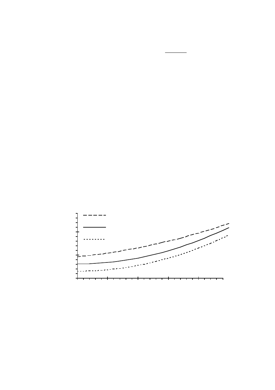
64
t
µ
max
(n
g
') = t
µ
ss max
+ (t
µ
N max
– t
µ
ss max
)
n
g
' + n
g
'
2
2
(3.31)
The worst case minimum torque is assumed to have no first-order term.
Minimum torques at rated speed and standstill are used as parameters
t
µ
min
(n
g
') = t
µ
ss min
+ (t
µ
N min
– t
µ
ss min
) n
g
'
2
(3.32)
If the model torque function and the estimated maximum and minimum
torque functions are plotted in the same diagram, an estimation of the model
error can be made, see Figure 3.4. In this case the error in the rated friction
torque, t
µ
N
, is assumed to be
±
20 %. The error in the standstill friction torque,
t
µ
ss
, is assumed to be
±
50 %. The total error of the friction and windage model
is found to be about 0.25 times the friction torque at rated speed
∆
T
µ
= 0.25 T
µ
N
= 0.25 ( t
µ
N
T
N
)
(3.33)
Generator speed (p.u.)
0,00
0,25
0,50
0
0,25
0,5
0,75
1
µ
max
µ
model
µ
min
t
t
t
Friction and windage torque
in percent of rated torque
Figure 3.4
The model friction and windage torque and the estimated
maximum and minimum limits for the torque.
Error in the core losses
The core loss torque model has two parameters: the core loss torque at rated
load t
Fe N
and the eddy current constant C
Ft
. The model of the core loss
torque is
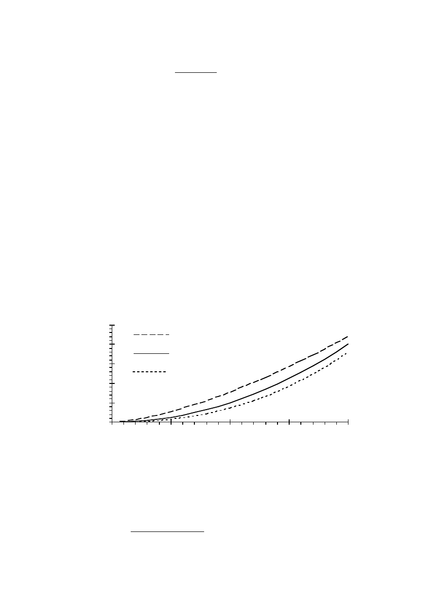
65
t
Fe
(n
g
',
ψ
) =
t
Fe N
ψ
2
1 + C
Ft
n
g
'
1 + C
Ft
(3.10)
It is a product of the hysteresis loss torque and the eddy current factor.
These two parts have different types of error. The parameters maximum and
minimum value have to be estimated: t
Fe N min
, t
Fe N max
, C
Ft min
and
C
Ft max
. First the error of the hysteresis loss torque is estimated. Using
x = 1.5 in Equation (3.4) and t
Fe N max
the maximum hysteresis loss torque is
t
Hy max
(
ψ
) ~
ψ
1.5
t
Fe N max
(3.34)
If x = 2.3 and t
Fe N min
is used the minimum hysteresis loss torque will be
t
Hy min
(
ψ)
~
ψ
2.3
t
Fe N min
(3.35)
The hysteresis loss torque at rated flux is assumed to have an error of
±
10 %.
From Figure 3.5 the error of the hysteresis loss torque can then be estimated
to be about 20 % of the hysteresis loss torque at rated flux. The worst case
error of the hysteresis loss approximation is at about 0.5 p.u. flux linkage.
Generator flux (p.u.)
Hysteresis torque (%)
0,0
0,5
1,0
1,5
2,0
2,5
0
0,25
0,5
0,75
1
Hy max
Hy model
Hy min
t
t
t
Figure 3.5
Model of hysteresis losses and an estimation of its error.
In Figure 3.6 the error of the eddy current factor is shown. The maximum
eddy current factor C
Fe max
is derived from Equations (3.3) and (3.5). In
Equation (3.3) y = 1.9 and C
Ft min
is used
C
Fe max
=
1 + C
Ft min
(n
g
')
0.9
1 + C
Ft min
(3.36)
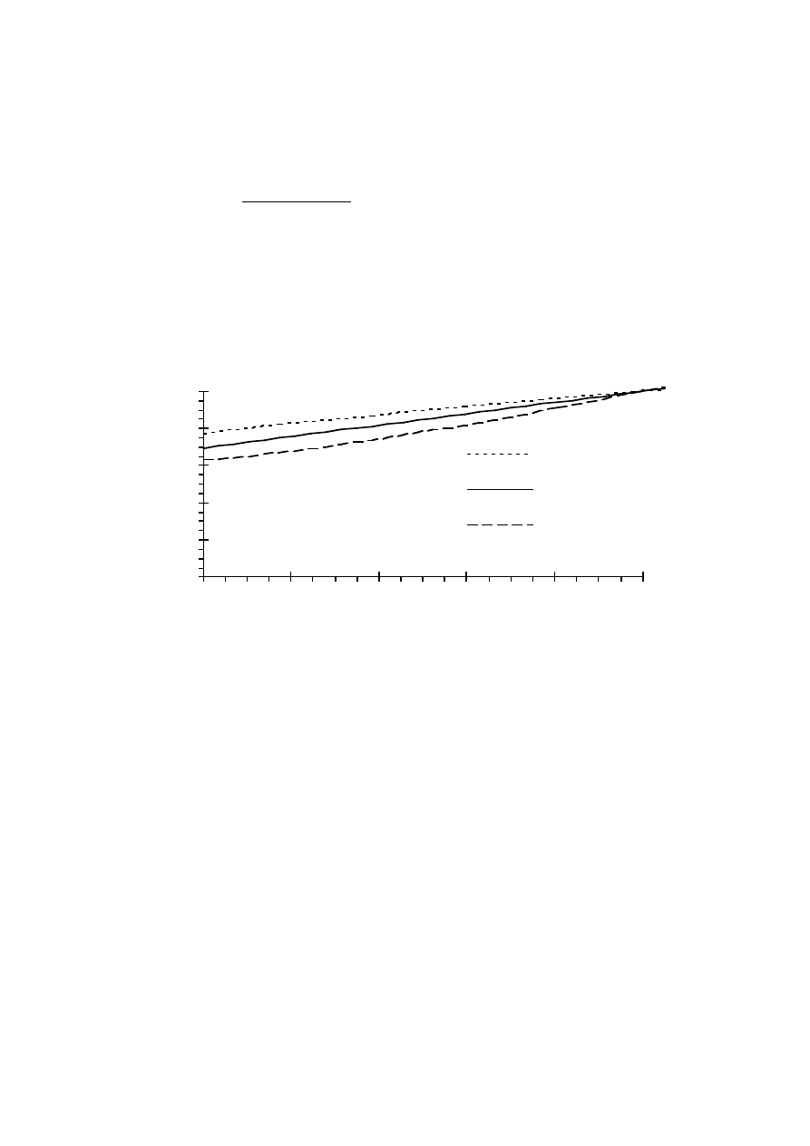
66
From the same equations the minimum eddy current factor can be derived if
y = 2.0 and C
Ft max
is used
C
Fe min
=
1 + C
Ft max
n
g
'
1 + C
Ft max
(3.37)
The error is larger at lower speed because the value of the core loss torque is
known at rated speed. The error in the total eddy current factor can be
estimated to be about 10 % when the error in C
Ft
is assumed to be about
20 %.
Generator speed (p.u.)
Eddy current factor
0,0
0,2
0,4
0,6
0,8
1,0
0
0,2
0,4
0,6
0,8
1
Fe max
Fe min
Fe
C
C
C
Figure 3.6
The simplified model of the eddy current factor and an
estimations of its maximum and minimum values.
The total error of the core loss model can be found as 20 % of the core losses
at rated load, due to the hysteresis torque error, plus 10 % of the actual core
losses, due to the eddy current factor error. These figures of the errors are
based on an error of the core losses at rated load of 10 % and an error of the
eddy current constant C
Ft
of 20 %. The total error is smallest at rated flux
and speed and larger at lower speed and lower flux. For simplicity the total
core loss error is assumed to be constant. In this example the core loss torque
error is
∆
T
Fe
= (0.20 + 0.10) T
Fe N
= 0.30 ( t
Fe N
T
N
)
(3.38)
Error in the winding losses
The theoretical formula for resistive losses can be assumed to be very
accurate. The largerst error of the resistive winding losses is due to the

67
temperature dependence of the winding resistance. In a normal wind turbine
generator the winding temperature can in the extreme case vary between
about –20˚ and +120˚ C. This gives a variation of the winding resistance of
±
25 % if a resistance value for 50˚ C is used. In a generator rated for a
temperature rise according to class B, max 80˚ C, it is however not usual
with winding temperature outside the range of +10˚ to +90˚ C. The change of
resistance is then
±
15 % if a resistance value for 50˚ C is used.
The error of the winding losses is estimated to be about
±
20 % of the actual
losses. About 15 % is due to normal temperature changes and about 5 % due
to an error in the measured winding resistance. The temperature of the
windings may under extreme weather conditions pass these limits giving a
larger error of the winding losses. In Sweden that will probably only occur for
some percent of the time. The errors of the resistive winding losses can be
expressed as
∆
P
Cu a
= 0.20 P
Cu a
= 0.20 ( 3 R
a
I
2
a
) = 0.20 ( r
a
i
2
a
P
N
) (3.39)
∆
P
Cu f
= 0.20 P
Cu f
= 0.20 ( R
f
I
2
f
) = 0.20 ( r
f
i
2
f
P
N
) (3.40)
If the error of the model must be reduced, the resistance value can be
changed according to a measurement of the winding temperature.
Error in the additional losses
Since the mechanisms of the additional losses are not investigated, the error
of their approximation can not be derived. If they are measured at rated load
the error can be estimated to be less than 50 %
∆
P
ad
= 0.50 P
ad
= 0.50 ( 3 R
ad
I
2
a
) = 0.50 ( r
ad
i
2
a
P
N
)
(3.41)
Total model error
The error of the power loss is smaller at partial load than at rated load and
the total error can be estimated as an error dependent on the speed, plus one
part that changes with armature current and one that changes with the field
current

68
∆
P
loss
P
N
=
n
g
∆
T
µ
n
g N
T
N
+
n
g
∆
T
Fe
n
g N
T
N
+
∆
P
Cu a
P
N
+
∆
P
ad
P
N
+
∆
P
Cu f
P
N
=
= ( 0.25 t
µ
N
+ 0.30 t
Fe N
) n
g
' + ( 0.20 r
a
+ 0.50 r
ad
) i
a
2
+ 0.20 r
f
i
f
2
(3.42)
The error of the calculated power loss decreases to zero if the speed,
armature current and field current all are decreasing to zero. The error can
also be expressed as a loss torque error
∆
T
loss
T
N
=
∆
T
µ
T
N
+
∆
T
Fe
T
N
+
∆
P
Cu a
/ n
g
P
N
/ n
g N
+
∆
P
ad
/ n
g
P
N
/ n
g N
+
∆
P
Cu f
/ n
g
P
N
/ n
g N
=
= (0.25 t
µ
N
+ 0.30 t
Fe N
) +
(0.20 r
a
+ 0.50 r
ad
) i
a
2
+ 0.20 r
f
i
f
2
n
g
'
(3.43)
From Equation (3.43) it can be seen that the torque error does not decrease
to zero even if the currents decrease to zero.
The higher the generator efficiency the lower the error is in the calculated
shaft torque, because the error is in percent of the losses and not in percent
of the power of the generator. The error described in this chapter is the model
error. The total error can be larger because of errors in the measurements of
the generator armature power, armature voltage, armature current, field
current and shaft speed. If an exciter is used there will also be an error in the
estimation of the field current.
3.2 Model of the converter losses
The converter losses have to be modelled to be able to compare the average
efficiency of a variable speed generator and converter system with the
average efficiency of a constant speed generator. The converter losses are
divided into rectifier losses P
loss r
, dc filter losses P
loss d
and inverter losses
P
loss i
. Losses due to the dc current ripple are neglected.
The losses of the diode bridge are due to the voltage drop in the semiconductor
material and to the switching losses. The voltage drop has two parts:

69
resistive voltage drop from the rectifier resistance R
r
and the no load voltage
drop U
0 r
. By including these two types of losses the total diode losses are
determined accurately enough since the switching losses are very small for
low frequency rectifiers. The rectifier losses are
P
loss r
(I
d
) = U
0 r
I
d
+ R
r
I
d
2
(3.44)
The suggested dc filter has two inductors and a capacitor bank. The losses in
the inductors are resistive losses and core losses. But the core losses are
relatively small in an inductor for a dc-current with ripple. The dominating
losses are the resistive ones in the winding. The capacitors have much lower
losses than the inductors have, only about some percent of the inductor
losses, and can therefore be neglected without introducing any significant
errors in the calculations. By adding the resistance of the two dc inductors
the dc filter losses can be expressed as
P
loss d
(I
d
) = R
d
I
d
2
(3.45)
where R
d
is the total resistance of the dc filter.
The thyristor losses are similar to the diode losses. The difference is that the
thyristor has a somewhat larger voltage drop. Using the same model as the
one for the diode bridge the thyristor inverter losses can be calculated. But
the inverter also has no-load losses P
0 i
from the cooling fan and the auxiliary
power supply to the control computer and the firing circuits. Therefore the
inverter losses are
P
loss i
(I
d
) = P
0 i
+ U
0 i
I
d
+ R
i
I
d
2
(3.46)
The total converter losses P
loss c
can be described as a sum of the no-load
losses of the inverter, the voltage drop losses of the diode rectifier and the
thyristor inverter and the resistive losses of the rectifier, dc filter and
inverter.
P
loss c
(I
d
) = P
0 i
+ (U
0 i
+ U
0 r
) I
d
+ (R
i
+ R
d
+ R
r
) I
d
2
(3.47)
The converter loss model error has not been estimated.
3.3 Model of the gear losses

70
The gear losses have not been measured. A theoretical model of the losses of
a normal gear is presented in [11]. The losses of the gear are divided into two
parts. The gear mesh losses which are a fixed percentage of the input power
independent of the gear shaft speed. The gear mesh losses are determined by
the design of the teeth of the cog-wheels. Friction losses are the other part of
the losses and they are mainly due to bearing friction, windage and oil
churning losses. The bearings, normally being roller bearings, give rise to an
almost constant breaking torque. Windage power losses are generally
proportional to the speed in cube. Expressed as a braking torque they are
proportional to the speed in square. The oil churning losses are difficult to
determine but the breaking torque should increase at least proportionally to
the rotational speed of the gear. If it is not known how the bearing, oil
churning and windage losses depend on the speed, a simplified function can be
used. It is certain that those losses increase at least linearly with the speed.
The following approximation of gear losses over-estimates the losses for all
speeds up to the rated speed
p
loss gear
(p
t
,n'
t
) = t
0 gear
n'
t
+ ( 1 –
η
mesh
) p
t
(3.48)
where t
0 gear
is the per unit friction torque at rated speed and
η
mesh
the gear
mesh efficiency.
3.4 Verification of the generator loss model
The losses are measured at various loads and under different conditions to
verify the loss model. A first step is to verify the generator loss model for
sinusoidal currents at resistive load. Then the model is used to predict the
losses for a diode loaded generator. The error when the loss model is used to
calculate the shaft torque from the armature power is also presented.
The losses are measured only indirectly by measuring the input mechanical
power and the output armature power of the generator. Therefore, the model
error is calculated as the shaft torque predicted by the model minus the
measured generator shaft torque.
When comparing the model and the measurements the error consists of two
parts. Besides the error of the model also the error due to the inaccuracy of
the measured variables will show in this comparison. The error in the torque

71
measurement is totally about 1.5 Nm. The predicted torque of the model is
also suffering from the error in the output power. The output power of the
generator is measured with a wattmeter that has an error of 0.5 % of the
actual power range. That range changes during the measurement but the
maximum error is always larger than 0.5 % of the actual power. The errors of
the measured variables for the loss model, like armature current and
generator speed, do not much affect the error of the predicted torque. The
total effect of the inaccuracy of the measurements is equal to about 3.0 Nm
at rated load and about 1.5 Nm at no load.
3.4.1 The laboratory system
Measurements were made on a system with the 50 kVA generator earlier
described. For that purpose a system with generator and frequency converter
or resistive three-phase load has been built in the laboratory. The laboratory
system and the measurement equipment used are shown in Figure 3.7. All
the measurements are made at steady state operation.
The generator is driven by a dc machine fed from a thyristor rectifier with
speed control. No gear is included in the laboratory system. On the shaft
between the dc motor and the synchronous generator the shaft torque and
speed are measured. The generator is magnetized mainly by sliprings but for
comparison it has also been magnetized by its integrated exciter. When it is
magnetized by the sliprings both the field current and the field voltage are
measured. The field current is fed from a current-controlled three-phase
thyristor rectifier via a fourth order LC-filter. The ripple on the field current is
only about one percent.
The exciter current is fed by a current regulating dc power supply. To be able
to find the relation between the exciter current and the field current the field
voltage is measured also when the exciter is used. From the field voltage and
the field resistance the field current can then be calculated.
The armature power is measured by a three-phase digital power meter
including harmonics up to 1 kHz. To estimate the generator flux at resistive
load the armature r.m.s. voltage is measured and to calculate the stator
winding copper losses the r.m.s. value of the armature current is also
measured.
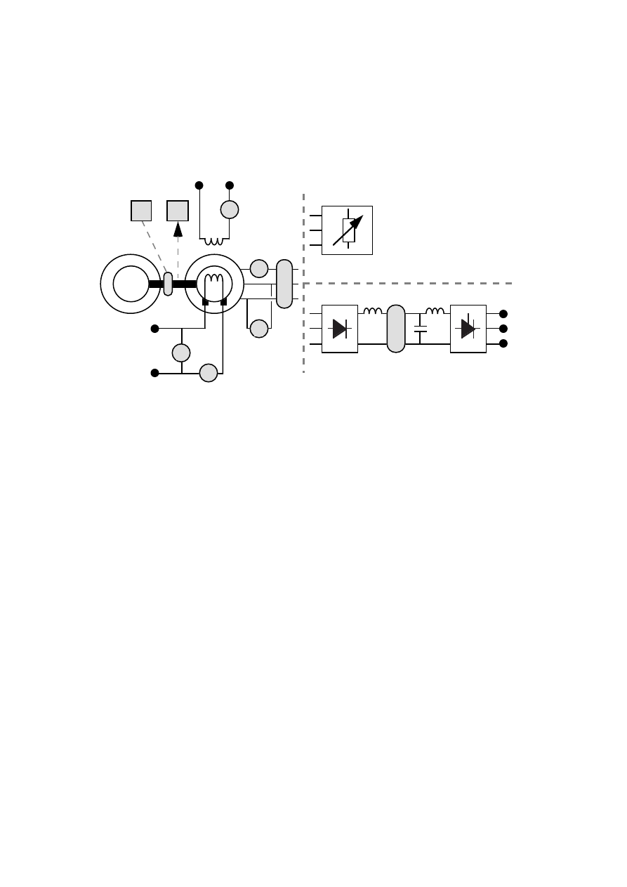
72
The generator power is either fed to a three-phase resistive load or to a
frequency converter. The frequency converter consists of a three-phase diode
rectifier, a dc filter and a thyristor inverter. In the dc filter the dc power as
well as the dc current and voltage are measured.
I
a
n
g
I
E
U
a
I
f
A
P
V
A
V
A
P
a
T
g
U
f
T
n
DC
Three-phase
resistive load
I
dr
U
d
P
U
I
P
d
Figure 3.7
The laboratory set-up with measurement instrumentation.
3.4.2 Parameter determination of the laboratory system
The per unit quantities are presented in Table 3.3 together with the
corresponding base values for the laboratory system. Note that the rated
values of the system are used as base values, and the rated values of the
generator can differ from these. There are also two current base values: one
for the field current and one for the armature current. All of the base values
in Table 3.3 can not be chosen independently. The power, speed and armature
current base values can be chosen. Then the torque, field current, flux linkage
and resistance base values can be calculated.
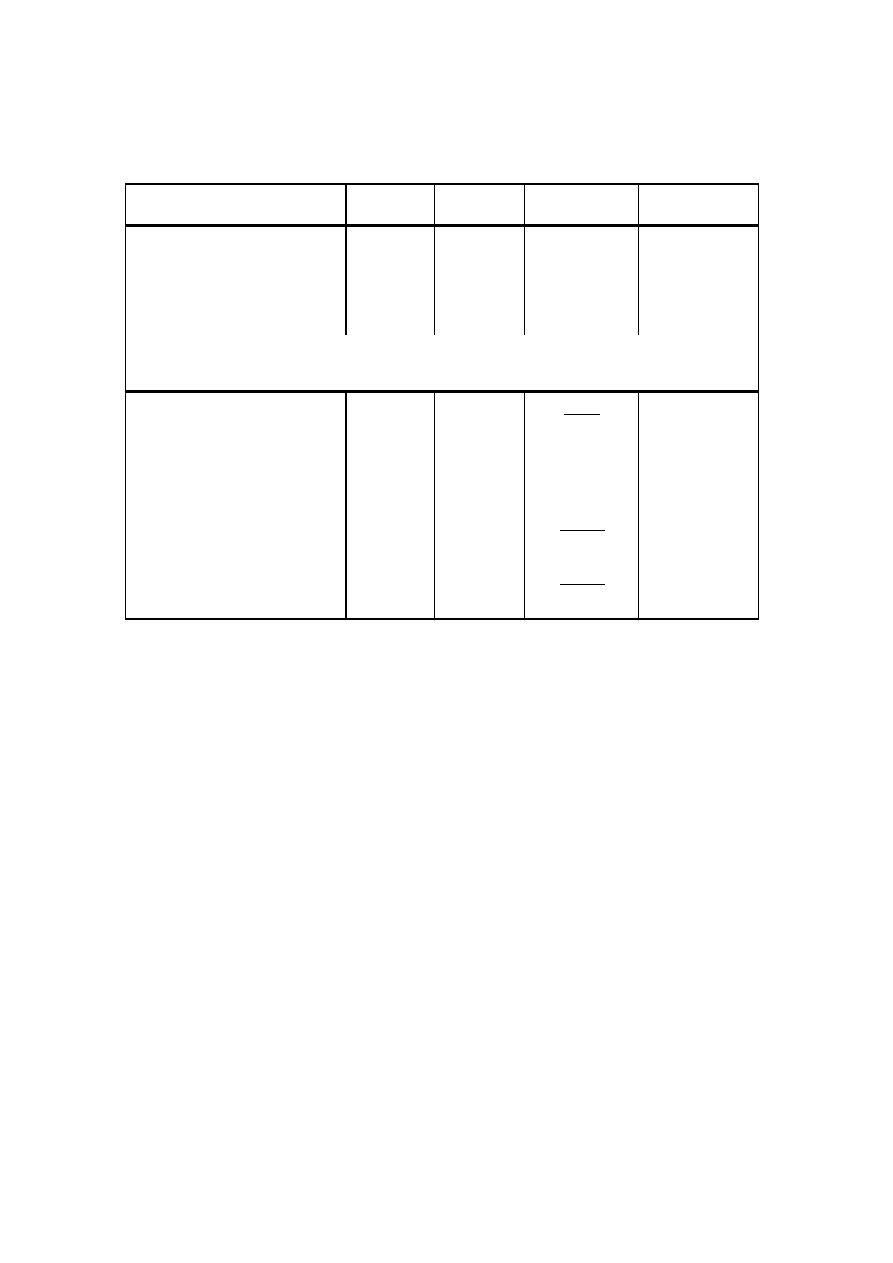
73
Table 3.3
The per unit quantities and their base values for the 50 kVA
generator.
Quantity
Notation
Per unit
quantity
Base
quantity
Base value
Mechanical power
P
g
p
g
P
g N
47 438 W
Shaft speed
n
g
n
g
'
n
g N
1500 rpm
Armature current
I
a
i
a
I
a N
78 A
Derived quantities:
Shaft torque
T
g
t
g
P
g N
n
g N
302 Nm
Field current
I
f
i
f
I
f N
19 A
Flux linkage
Ψ
ψ
Ψ
N
1.12 Vs
Armature resistance
R
a
r
a
P
g N
I
2
a N
2.60
Ω
Field resistance
R
f
r
f
P
g N
I
2
f N
122
Ω
Friction and windage losses
The friction and windage losses of the generator can be measured on an
electrically disconnected machine. They are simply measured as the input
shaft power at different speeds if there is no magnetic flux in the generator.
For the friction and windage loss model, only the friction and windage braking
torque at rated speed and at standstill have to be measured.
If the rotor can not be demagnetized the friction and windage torque can be
found from no load measurements at low magnetizations. The friction and
windage braking torque for a certain speed is found by extrapolating the
torque-voltage curve to zero voltage. In Figure 3.8 a torque-voltage curve for
1000 rpm can be seen, in which the friction torque at 1000 rpm is found as
the no-load torque extrapolated to zero voltage.
74
Armature voltage (V)
No-load torque (Nm)
0
2
4
6
8
10
0
50
100
150
200
250
300
T
µ
(1000 rpm)
I
f
= 0 A
I
f
= 15 A
I
f
= 12.5 A
I
f
= 10 A
I
f
= 7.5 A
I
f
= 5 A
I
f
= 2.5 A
Figure 3.8
A no-load torque-voltage curve used to find the friction loss torque
at 1000 rpm for the 50 kVA generator.
In Figure 3.9 the zero voltage torque from a number of such curves has been
plotted in the same diagram to form the torque-speed curve for the friction
and windage losses.
The standstill friction torque can be found by extrapolating the friction and
windage loss torque for low speeds down to zero speed. For the 50 kVA
generator the friction and windage parameters are
T
µ
ss
= 0.468 Nm
and
T
µ
N
= 1.694 Nm
(3.49)
t
µ
ss
= 0.155 %
and
t
µ
N
= 0.407 %
(3.50)
Generator speed (rpm)
Friction torque (Nm)
0
0,5
1
1,5
2
2,5
0
500
1000
1500
T
T
µ
N
µ
ss

75
Figure 3.9
The torque-speed points from measurements of the friction and
windage losses of the 50 kVA generator, and the model function
drawn as a line.
Core losses
Measurements made at different speeds are necessary for separating the
hysteresis losses and the eddy current losses. From no-load measurements
the core losses can be calculated as the input mechanical power minus the
friction losses. First the eddy current constant is determined and then the
hysteresis loss torque is determined.
To separate the hysteresis losses from the eddy current losses the measured
total core loss torque is plotted as a function of the generator speed for some
fixed values of the field current. At no load a fixed field current is equal to a
fixed flux linkage. The measured core loss torque for the 50 kVA generator is
shown in Figure 3.10. The hysteresis torque can be determined if the curve is
extrapolated to zero speed. The speed dependency of the data should form
straight lines, according to Equation (3.10). Figure 3.10 shows that the speed
dependency for high flux is not linear, especially not for low speeds of the
generator. But if the model is to be used in a wind turbine generator system,
speeds below 500 rpm will be of no interest. The curve fit should be made only
for the data between the lowest and the highest speeds used in that
particular wind turbine generator system.
Based on the measured data, it is possible to get one value of the eddy
current constant for each value of the flux linkage (field current). The eddy
current constant can for each flux linkage be calculated by the following
equation
C
Ft
(
Ψ
) =
T
Fe
(
Ψ
,1500 rpm) – T
Fe
(
Ψ
,0 rpm)
T
Fe
(
Ψ
,0 rpm)
(3.51)
The value of the eddy current constant used in the model is the mean value of
the constants for the different flux linkages. The results can be found in Table
3.4. The mean value of the eddy current constant is calculated
C
Ft
= 0.44
(3.52)
76
Generator speed (rpm)
Core loss torque (Nm)
0
2
4
6
8
10
0
500
1000
1500
If=25.0 A
If=20.0 A
If=15.0 A
If=12.5 A
If=10.0 A
If= 7.5 A
If= 5.0 A
If= 2.5 A
Operating speed range
T
Fe
(
Ψ
,0 rpm)
T
Fe
(
Ψ
,1500 rpm)
Figure 3.10 The core loss torque of the 50 kVA generator versus the generator
speed for some fixed field currents.
The variation in the eddy current constant C
Ft
with flux linkage is as large as
±
25 % according to Table 3.4, but the resulting error in the total eddy current
factor (1 + C
Ft
n
g
') is much smaller. It is less than 3.5 % as can be seen in
Figure 3.11. This small error is achieved by determining the hysteresis torque
from the data in the middle of the used speed range. The eddy current factor
is then correct for that speed, here 1000 rpm.
Table 3.4
The eddy current constant for different flux linkages and the mean
value used.
I
f
(A)
Ψ
(
Vs
)
T
Fe
(
Ψ
,1500 rpm)
(
Nm
)
T
Fe
(
Ψ
,0 rpm)
(
Nm
)
C
Ft
(
Ψ
)
2.5
0.45
1.00
0.72
0.389
5.0
0.81
2.55
1.78
0.431
7.5
0.99
3.64
2.54
0.433
10.0
1.07
4.39
2.86
0.536
15.0
1.13
5.24
3.36
0.536
20.0
1.23
7.78
5.58
0.394
25.0
1.27
9.47
7.12
0.330
mean value
⇒
0.44
77
Generator speed (rpm)
Eddy current factor
1
1,2
1,4
0
500
1000
1500
C
C
C
Ft min
Ft max
Ft
Figure 3.11 The error of the eddy current factor.
To find the relation between the hysteresis loss torque and the flux linkage,
the core loss torque from the measurement above is used. The core loss
torque is plotted versus the flux for one speed. The speed that should be used
is the one in the middle of the used speed range of the wind turbine generator
system. This is neccesary in order to reduce the error of assuming that all the
torque-speed lines have the same slope. For the 50 kVA generator the speed
range is 500 to 1500 rpm, and the hysteresis loss torque is therefore
approximated from the loss torque at 1000 rpm. To reduce the absolute error,
the values of the core loss torque should be taken from the straight lines that
already have been used to approximate the eddy current factor, not directly
from measurements at 1000 rpm. The chosen core loss torque values do not
only contain the hysteresis torque but also the eddy current torque, in this
case the eddy current torque of 1000 rpm. The eddy current loss torque is
excluded before the curve fit is made by using the formula for the relation
between hysteresis losses and eddy current losses at different speeds
T
Hy
(
Ψ
) =
T
Fe
(
Ψ
,1000 rpm)
1 + 0.44
1000 rpm
1500 rpm
(3.53)
After the division by the eddy current factor the hysteresis losses at rated
flux linkage can be found. The measured hysteresis loss torque as well as the
model of it is shown in Figure 3.12. The hysteresis loss torque may have a
very steep increase when the flux exceeds the rated flux linkage.
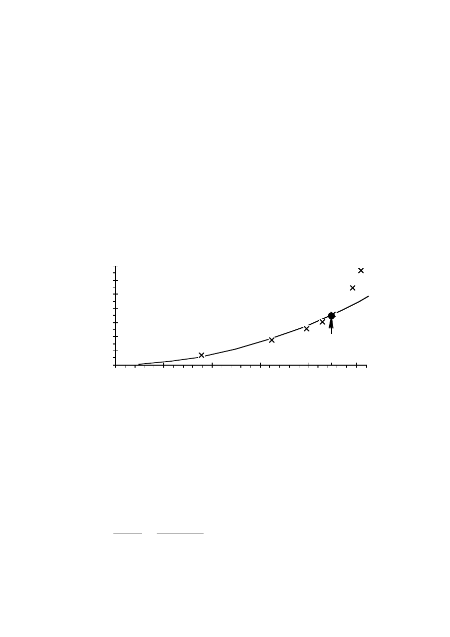
78
The model parameter for the hysteresis loss torque of the 50 kVA generator
is
T
Hy N
= 3.47 Nm
(3.54)
and in per unit the hysteresis loss torque is
t
Hy N
= 1.15 %
(3.55)
The parameter t
Fe N
for the model can now be calculated
t
Fe N
= t
Hy N
( 1 + C
Ft
) = 1.15 % ( 1 + 0.44 ) = 1.656 %
(3.56)
Generator flux linkage (Vs)
Hysteresis torque (Nm) 0
1
2
3
4
5
6
7
0,00
0,25
0,50
0,75
1,00
1,25
Rated
flux
Fe N
t
Figure 3.12 The model of and the measured hysteresis loss torque.
Armature resistance
For the 50 kVA generator the armature resistance is 66 m
Ω
per phase. The
resistive losses can then be expressed in per unit of the rated generator
power as
r
a
=
P
cu a N
P
g N
=
3 R
a
I
a N
2
P
g N
= 2.54 %
(3.57)
79
Field winding resistance
For the 50 kVA generator the field winding resistance is 1.37
Ω
which make
the per unit field winding resistance
r
f
=
P
cu f N
P
g N
=
R
f
I
f N
2
P
g N
= 1.04 %
(3.58)
Exciter rotor resistance
The per phase resistance of the exciter armature was measured by
disconnecting the rotating diode rectifier
R
a E
= 0.135
Ω
(3.59)
r
a E
=
P
cu E N
P
g N
=
2 R
a E
I
f N
2
P
g N
= 0.21 %
(3.60)
Additional losses
The additional losses in the generator are smaller than the measurement
accuracy of the laboratory system, which makes it difficult to trace them
from single measurements. Instead the error of the loss model is plotted as a
function of armature current, when no additional losses are included in the
model. At resistive load no systematic correlation is found between the error
of the model and the armature current, see Figure 3.13. Thus the additional
losses can be assumed to be close to zero.
Armature current (A)
Power error (W)
-500
-250
0
250
500
20
40
60
80
Figure 3.13 The model error at resistive load, when additional losses are not
modelled.
80
The additional losses at diode load are also small compared with the
measurement accuracy and can not be exactly determined, see Figure 3.14.
Measurements at 1500 rpm show that the additional losses can be estimated
to about 320 W at rated armature current. The additional losses at diode load
can be represented by an equivalent armature resistance
r
ad
=
P
ad N
P
g N
= 0.67 %
(3.61)
Dc current (A)
Additional losses (W) -1200,0
-900,0
-600,0
-300,0
0,0
300,0
25
50
75
100
P
ad N
Figure 3.14 The model error at diode load, when additional losses are not
modelled. The additional losses can be found as the current-
dependent part of the loss model error. An approximation of the
additional losses is also shown as a line.
Error in the model for the 50 kVA generator
The total error in percent of the rated power is, according to Equation (3.42)
∆
P
loss
P
N
= (0.14 % + 0.50 %) n
g
'+ (0.51 % + 0.34 %) i
a
2
+ 0.21 % i
f
2
(3.62)
The error expressed as a percentage of the rated shaft torque is, according to
Equation (3.43)
∆
T
loss
T
N
= 0.14 % + 0.50 % +
1
n
g
'
[
]
(
)
0.51 % + 0.34 % i
a
2
+ 0.21 % i
f
2
(3.63)
81
The maximum error in the loss model is, for the 50 kVA generator, about
1.7 % of the rated generator power at rated load. The error of the calculated
shaft torque is also 1.7 % of the rated shaft torque.
3.4.3 Verification of the exciter losses
In Figure 3.15 the exciter losses plus field winding losses have been calculated
from the measurements. It can be seen that only the resistive losses in the
rotor must be included in the model.
Field current (A)
Rotor and exciter losses
(W)
0
500
1000
1500
0
10
20
30
Exciter and
rotor losses
Calculated
resistive
rotor losses
Figure 3.15 The losses of the exciter and main field winding versus main field
current.
3.4.4 Model error at resistive load
To find out how accurate the loss model is, first the error between the model
and the measured losses is calculated for the generator with resistive load. In
the next section the same comparison is made for the generator loaded by a
diode rectifier.
The losses are measured at all the combinations of five different generator
speeds, five different armature currents and five different generator flux
linkages. That is a total of 125 different load combinations that cover all
possible loadings of the generator. For each measurement the generator
speed, shaft torque, field current, field winding voltage, armature voltage,
armature current and electrical output power are measured. The model error
is defined as the shaft power or torque predicted by the model minus the
measured shaft power or torque.
82
For the resistivly loaded generator no additional losses are included in the
model. The torque error is always less than the total measurement error,
±
3 Nm. So, just by looking at the magnitude of the error it can not be judged
whether the error depends on the model or the inaccuracy of the
measurement. But if the error is plotted versus for instance the generator
current, the generator flux linkage or the speed it will be possible to see if
there are any correlation between the errors and different quantities. By
looking at how the error changes with a certain quantity, it shows if there are
systematic errors even if those errors are smaller than the stochastic ones.
The model torque error is plotted versus the generator shaft speed. It can be
seen that the magnitude of the error is almost independent of the speed, see
Figure 3.16. The mean value of the model error is not perfectly zero for all
speeds but it is such a small correlation to the speed that it is well within
what should be expected.
Generator speed (rpm)
Torque error (Nm)
-3
-2
-1
0
1
2
3
500
1000
1500
2000
Figure 3.16 The torque error at resistive load and at different generator speeds.
The error plotted versus the generator flux linkage, Figure 3.17, shows a
definite correlation between the error and the flux linkage. At low generator
flux linkage the model underestimates the losses and at high flux linkage it
overestimates them. This is probably difficult to correct without a lot of
calculations for each new generator to be modelled. However, the error is also
here small and well within the desired accuracy of the model.
83
Flux linkage (Vs)
Torque error (Nm)
-3
-2
-1
0
1
2
3
0
0,25
0,5
0,75
1
1,25
Figure 3.17 The torque error at resistive load and at different generator flux
linkages.
It can be seen, in Figure 3.18, that the size of the power error is to a large
extent depending on the armature current but the mean value of the error is
close to zero for all currents, so the model can not be corrected by changing
for instance the resistance value.
Armature current (A)
Power error (W)
-500
-250
0
250
500
20
40
60
80
Figure 3.18 The power error at resistive load and at different armature
currents.
All the model and measurement errors with resistive load are less than 3 Nm
which is about 1 % of the rated torque or or 500 W which is about 1 % of the
rated power. The measurement errors can amount to 1 % so it is not possible
to say how large the actual model error is.
84
3.4.5 Model error at diode load
When the generator is loaded by a diode rectifier the losses increase a little
compared with resistive load. The increase is expected, since there will be
losses in the damper windings that do not occur at resistive load. There will
also be more harmonics in the stator current leading to higher copper losses.
Because of the larger proportion of high frequency components in the flux
distribution the eddy current losses increase more than the hysteresis losses.
At resistive load the additional losses are low enough to be neglected. To take
the additional losses into account at diode load the model now includes a
fictitious armature resistance representing the additional losses. The error of
the calculated shaft torque is plotted for different speeds, dc current, and
generator flux linkage.
Figure 3.19 show the model torque error for some speeds, it can be seen that
the error changes with the speed. The loss model underestimates the losses
at higher speeds which indicates that the eddy current losses have increased
compared with no-load. The speed dependence of the error is larger than that
at resistive load: compare Figures 3.16 and 3.19.
Generator speed (rpm)
Torque error (Nm)
-6,0
-3,0
0,0
3,0
6,0
500
1000
1500
2000
Figure 3.19 The torque error at diode load and at different generator speeds.
Figure 3.20 shows no simple correlation between the generator flux linkage
and the torque error. The correlation is different from that at resistive load,
compare Figures 3.17 and 3.20. The difference may depend only on the fact
that there are different ways of calculating the flux linkage with resistive load
and with diode load.
85
Flux linkage (Vs)
Torque error (Nm)
-6,0
-3,0
0,0
3,0
6,0
0
0,25
0,5
0,75
1
1,25
Figure 3.20 The torque error at diode load and at different generator flux
linkages.
The armature current clearly effect the magnitude of the power error in the
same way as it does at resistive load, compare Figures 3.18 and 3.21.
Although the additional losses are taken into account, the model is not as
accurate at diode load as it is at resistive load. The total error when
comparing model and measurements is, for a diode-loaded generator, up to
2 % of the rated power or torque. The measurement error can contribute with
no more than 1 %.
Dc current (A)
Power error (W)
-900,0
-600,0
-300,0
0,0
300,0
25
50
75
100
Figure 3.21 The error in estimated power at different dc currents.
3.4.6 Error in the torque control
The loss model can be used for torque control of the generator. The error of
such a torque control is easiest found if the torque error of the model is plotted
with the measured shaft torque as a parameter. Since the model is intended
86
for use in a variable speed wind turbine generator system only the error at
diode load is presented here. In Figure 3.22 the torque error is plotted for all
possible combinations of speed, armature current and flux linkages.
Shaft torque (Nm)
Torque error (Nm)
-6,0
-3,0
0,0
3,0
6,0
100
200
300
Figure 3.22 The error, at diode load, in the calculated torque compared with
the actual torque, for all possible combinations of speed, armature
current and flux linkages.
In this comparison of torque error versus shaft torque the error is almost
zero at zero torque, but this is because the parameters for the friction losses
and core losses are measured. If they were estimated with an error, that
would show as an offset error at zero shaft torque. The error decreases for low
shaft torque, but not linearly with the torque. This means that the total error
will never be more than about 2 % of the rated generator torque but the
relative torque error can be larger than 2 % at part load.
In a wind turbine generator system not all of the above measured load
combinations are realistic. For instance, high current at high flux linkage and
low speed will never occur. Since the most extrem load combinations have the
largest errors it is interesting to find the error of only the load combinations
that will be used in a wind turbine generator system. These load
combinations follow the torque-speed curve of the optimum load of a wind
turbine. For wind turbine loads it can be seen that the model error is generally
smaller than for other loadings, see Figure 3.23. Large errors only occur with
low flux linkage combined with high current, probably due to armature
reaction effects. If these low magnetizations are avoided the maximum error
will be less than 1 % percent for the 50 kVA generator.
87
Shaft torque (Nm)
Torque error (Nm)
-8
-6
-4
-2
0
2
4
100
200
300
Normal flux linkage
Low flux linkage and high
armature reaction
Figure 3.23 The torque error of the model with normal wind turbine loads.
Normal flux linkage (filled dots) and low flux linkage and high
armature reaction (unfilled dots).
3.5 Model for the 300 kW design example
In the following chapters, the loss model is used in the design of the system
and to calculate the average efficiency of the generator and converter
system. These calculations are made for the 300 kW design example system
and here the parameters for that system are derived.
3.5.1 Generator parameters
For the 300 kW generator with exciter the loss model can be determined
mainly by data from the manufacturer [12], but also with estimations based
on scaling of known data. In Table 3.5 the 50 and 60 Hz data from the
generator manufacturer are presented. The data are also recalculated for the
lower rated current and voltage used in the design example system. Some
parameters have only been estimated.
The parameters of the simplified loss model for the 300 kW generator can
now be determined. The friction and windage torque parameters are
estimated to
t
µ
N
= 0.66 %
(estimated)
(3.64)
t
µ
ss
= 0.22 %
(estimated)
(3.65)
88
Table 3.5
Data for the design example generator. Data are available for
class H loading at 50 and 60 Hz and those are recalculated for the
ratings used in the design example.
Data for
synchronous gen.
LSA 47.5 M4
50 Hz
1500 rpm
60 Hz
1800 rpm
design example
1800 rpm
Temperature rise
class H
class H
class B
S
a N
350 kVA
420 kVA
334 kVA
P
g N
≈
320 kW
I
a N
505 A
505 A
410 A
U
a N
/ n
N
400 V/1500
rpm
480 V/1800
rpm
475 V/1800
rpm
P
loss 0
(No load losses)
5400 W
7600 W
7600 W
x
d
"
13.7 %
14.3 %
11.7 %
x
q
"
17.4 %
18.1 %
14.8 %
R
a
(at 50˚ C)
0.0128
Ω
0.0128
Ω
0.0128
Ω
x
s
≈
x
d
355 %
370 %
304 %
Estimated losses:
n
g N
T
µ
N
1480 W / 0.4 % 2100 W / 0.48 %
2100 W / 0.66
%
P
ad N
1940 W / 0.52
%
1940 W / 0.44 % 1280 W / 0.4 %
P
Cu f N
4200 W / 1.2 % 4200 W / 0.95 % 2900 W / 0.9 %
The field winding losses at no load are very small even at rated flux. The large
synchronous reactance makes the no load field current only about 25 % of
the rated field current. Therefore, the field winding losses at no load, p
Cu f 0
,
are only 6 % of the field winding losses at rated load and they are neglected.
The core loss torque at rated flux can be determined approximately from the
no load losses as
t
Fe N
=
p
loss 0
– p
Cu f 0
n'
g N
– t
µ
N
=
{
}
p
Cu f 0
≈
0
≈
1.72 %
(3.66)
No value of C
Ft
has been found and for this example it is estimated to be
C
Ft
= 0.5
(estimated)
(3.67)

89
r
a
=
3 R
a
I
a N
2
P
g N
= 2.02 %
(3.68)
r
ad
=
P
ad N
P
g N
= 0.40 %
(estimated)
(3.69)
r
f
=
P
Cu f N
P
g N
= 0.90 %
(3.70)
R
r com
=
1
2
x
r com
=
1
2
x
d
" + x
q
"
2
= 6.58 %
(3.71)
x
s
= 304 %
(3.72)
3.5.2 Converter parameters
For the design example system the converter losses are in Chapter 2 found to
be
p
loss c
(i
d
) = 0.12 % + (0.52+0.33) % i
d
+ (0.10+0.70+0.17) % i
d
2
(3.73)
The converter efficiency at rated load is 98 %.
3.5.3 Gear parameters
A gear in the 300 kW range would have gear mesh losses of about 1 % for
each stage and friction losses of about 0.5 % at rated load and at rated speed.
In this model the gear friction torque is assumed to be constant. The braking
torque of the gear losses, for a gearbox of 97 % rated efficiency, is
t
loss gear
(t
t
) = 0.5 % + 2.5 % t
t
(3.74)
where
t
t
is the turbine shaft torque in per unit.

90
4 The use of the loss model in control and design
In this chapter, the system efficiency is optimized. The model of losses in the
generator and converter can be used to maximize the efficiency of the system
during operation. The system design can also be optimized by comparing
different generators of various rated power and rated speed.
4.1 Optimum generator voltage control
The frequency converter does not only allow variations in the generator
frequency. It also allows variations of the generator voltage. In a wind turbine
generator system the optimum shaft torque is pre-determined as a function
of speed. The optimum torque can, however, be obtained by different
combinations of generator current and voltage. This control possibility can be
used to minimize the generator and converter losses by means of the voltage
control.
The maximum allowed generator voltage is limited by the inverter ac voltage
at full load and at low load and low speed by the maximum allowed generator
flux. At full load the generator voltage is limited to 90 % of the inverter ac
voltage to insure safe commutation of the inverter. At low load and low speed
the generator flux has to be lower than 105 % of the rated generator flux and
this limits the generator voltage. According to standards the generator must
be able to continuously operate at a flux 5 % higher than the rated value [13].
On the other hand, the generator voltage may not be so low that the
armature current increases above its rated value. Within these limits, the
voltage can be controlled freely.
The generator core losses decrease with decreasing flux and the armature
copper losses decrease with decreasing current. Also the field winding losses
change with the flux. If the armature reaction is small, the field winding
losses will decrease with decreasing voltage, and if it is high the field winding
losses will increase with decreased voltage. The increase in field winding
losses at high armature reaction occurs because the field current must
increase to balance the increasing armature currents even though the
voltage is decreased. Also the efficiency of the converter changes with the
voltage. Since most of the losses are due to voltage drops of the
semiconductors and resistive voltage drops of the dc filter, the losses increase
with increasing current. For a fixed power the converter losses thus increase
with decreasing voltage. The generator voltage should be controlled to
91
minimize the sum of core losses, field winding losses, copper losses and
converter losses, see Figure 4.1.
0.2
0.4
0.6
0.8
1
Dc voltage (p.u.)
0
0.01
0.02
0.03
0.04
0.05
Generator and converter losses (p.u.)
Total losses
Armature losses
Converter losses
Field winding
losses
Core losses
Optimum
voltage
Figure 4.1
The core losses, field winding losses, armature copper losses,
converter losses and the total losses versus dc voltage at a fixed
speed and power.
In Figure 4.2 the total generator and converter efficiency versus the input
power of the generator can be seen both when an optimized voltage control is
used and when the flux is kept constant at the rated flux.
From the loss model the optimum voltage-speed curve can be calculated
theoretically. This curve is together with the voltage limits shown in
Figure 4.3. If low voltages are used, there may be problems with the voltage
control even if the current is not higher than the rated current. These
problems arise because the armature reaction eventually becomes
dominating in the generator voltage control. Normally, the voltage is reduced
by reducing the field current. At the same time, the armature current is
increased to keep the shaft torque constant. But, if the armature reaction is
large, it may be necessary to raise the field current when the armature
current is increased even though the voltage is reduced. The coupling between
the voltage control and the current control may in that case cause problems.
92
0.2
0.4
0.6
0.8
1
Generator input power (p.u.)
0.65
0.7
0.75
0.8
0.85
0.9
Generator and converter
efficiency
Optimized voltage control
Constant rated flux
Figure 4.2
The generator and converter efficiency versus generator input
power using an optimized voltage control and using constant
rated flux.
0.2
0.4
0.6
0.8
1
Wind speed (p.u.)
0
0.2
0.4
0.6
0.8
1
Generator voltage (p.u.)
Maximum voltage
Minimum voltage
Voltage at maximum efficiency
Figure 4.3
The maximum, optimum and minimum voltage of the generator
in a variable speed wind turbine generator system.
4.2 Efficiency as a function of generator size
The generator rating should be chosen to minimize the total cost of both the
generator and its losses. A large generator may be the most economic choice,
even though it is more expensive, if it is more efficient.

93
When comparing data for different sizes of the same generator type, e.g. for
Leroy Somer generators [12], it can be seen that the different per unit losses
do not always decrease when the size of the generator increases, because the
generators are made in different standard frame sizes. Increasing the rated
efficiency is not always done by increasing the generator frame size. When
comparing the losses between two close generator sizes the smaller
generator may, therefore, sometimes have lower armature resistance
although its rated current is smaller. But only on very rare occasions it can
be found that a generator has a lower rated efficiency than one that is
smaller.
The efficiency of three generators of different sizes is compared. It is
assumed that they have the same efficiency at their respective rated
powers. The generator sizes are chosen so that one generator will have a
rated power of only 80 % of the wind turbine generator system maximum
power. The rated power of the next generator is 100 % and of the last
generator 120 % of the maximum turbine power. In Figure 4.4 the efficiency
is plotted and it is clear that an oversized generator does not have higher
efficiency if the per unit losses are equal. An undersized generator has the
highest efficiency but it can of course not be used because it will be
overloaded. A larger generator will give a higher efficiency only if the increase
of rated efficiency is larger than the decrease in efficiency by reducing the
generator per unit load. At a certain power the difference in efficiency
between generators of different sizes can generally be expected to be small.
An other reason to use a larger generator than necessary would be, besides a
higher generator efficiency, that the insulation limit the generator life. Since
the generator in a wind turbine generator system should have a very long
operational life compared with many motor applications, the rating for the
temperature class H or F may be too high leading to isolation failure after
less than 20 to 30 year. A generator, made with class H insulation, can
instead be used with a rated power that only leads to temperature rises
according to class B to increase the life of the insulation. This is the same as
using a larger generator for a specific power.
94
0.2
0.4
0.6
0.8
1
Generator input power (p.u.)
0.88
0.89
0.9
0.91
0.92
0.93
0.94
Generator efficiency
20% larger generator
Normal generator size
20% smaller generator
Figure 4.4
The efficiency of generators of different rated power.
4.3 Optimum generator speed
For network-connected ac generators only some few fixed speeds can be used.
These speeds are determined by the network frequency and the number of
pole pairs of the generator. For a 50 Hz network the available speeds are
3000, 1500, 1000, 750 rpm and lower.
For a variable-speed wind turbine generator system the choice of the
generator speed is not restricted to a choice of pole pair number. The
frequency of the generator can also be chosen freely which allows any
generator speed. For instance, a four-pole generator can either be used at
1200 rpm and a frequency of 40 Hz or at 1800 rpm and 60 Hz. A six-pole
generator can also be used at 1800 rpm and the frequency is then 90 Hz.
Even though the turbine speed is determined by its optimum tip-speed ratio,
the speed of the generator can be changed by using different gear ratios.
From the loss model it can be found how the efficiency change with the
generator speed. The change in efficiency when the speed is changed depend
on how the power and generator flux are changed with the speed. Two
comparisons are made. First the generator efficiency is calculated at various
speeds but at constant power and secondly the generator efficiency is
calculated when it is loaded as much as possible at each speed.
95
When the power of the generator is the same at all different speeds the
armature voltage can be kept constant. If the voltage is constant, the flux of
the generator will be approximately inversely proportional to the speed of the
generator. The power being constant as well as the voltage leads to a
constant armature current. The friction and windage losses increase almost
by the speed raised to a power of three. Armature winding copper losses
remain constant in this example since the current is constant. The flux is,
however, reduced which reduces the hysteresis losses. Also the eddy current
losses are reduced but not as much as the hysteresis losses. Field winding
losses are reduced too, because of the reduced flux.
The efficiency can, however, be better optimized by controlling the voltage to
maximize the efficiency for each generator speed. Calculations on the
efficiency with this type of control are also made. The armature current is
now decreased a little as the speed increase since the voltage may increase.
Not only the core losses and field winding losses decrease but also the
armature copper losses.
The loss model of the generator is used to calculate the efficiency versus the
speed of the generator at a fixed input power. The resulting efficiency for the
50 kVA generator used at a constant voltage or at a voltage controlled to
maximize the efficiency can be seen in Figure 4.5.
1
1.2
1.4
1.6
1.8
2
Generator speed (p.u.)
0.91
0.92
0.93
0.94
0.95
Generator efficiency
Maximum efficiency
Constant voltage
Figure 4.5
The theoretical efficiency of the 50 kVA generator at a constant
power.
96
In the diagram it can be seen that the efficiency of the 50 kVA generator at
diode load has its peak value for a speed of 1.1 p.u., if the voltage and power
are both kept constant. The efficiency is then 93.7%. If the efficiency is
optimized by raising the voltage, the efficiency can be even higher, 94.1%,
and have its peak value at 1.25 p.u. speed. It is clear that the generator
speed should be kept high to increase efficiency. A realistic limit is probably
1800 rpm, that is equal to 1.2 p.u.
The speed dependency of the generator efficiency will not be the same if the
power of the generator is allowed to increase with the speed, see Figure 4.6.
This calculation is interesting because it shows how the generator efficiency
changes if the generator is always maximally utilized. To avoid overcurrent in
the windings the voltage must at least be raised proportionally to the
generator speed, corresponding to a constant flux.
1
1.5
2
2.5
Generator speed (p.u.)
0.91
0.92
0.93
0.94
0.95
Generator efficiency
Maximum efficiency
Constant flux
Figure 4.6
The theoretical maximum efficiency of the 50 kVA generator at its
maximum power.
If the generator is fully utilized, the efficiency will be even higher than if the
power is kept at its rated value for 1500 rpm. The maximum efficiency is
94.6 % but it is at a speed far too high for ordinary generators, 2.2 p.u. Using
rated generator flux the maximum generator efficiency is only slightly lower
and at a speed of 2.05 p.u. These theoretical maximum efficiencies cannot be
reached because the generator will be overloaded. It is, however, clear that a
high speed and a high utilization increase generator efficiency.
The results above show how the generator efficiency changes with the
generator speed. The converter efficiency does not depend on the speed of the
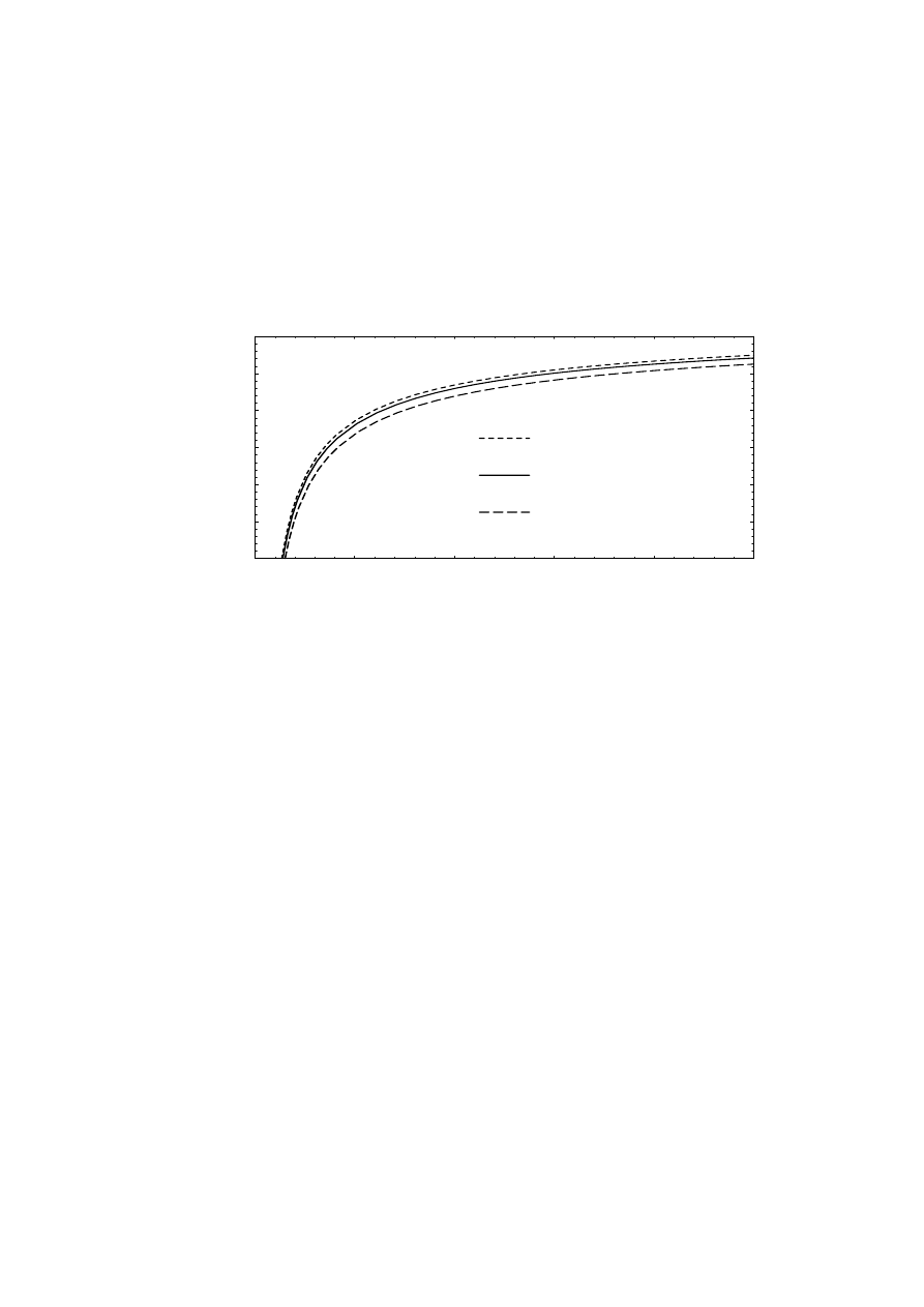
97
generator, only on the rated voltage. The rated voltage is determined by the
network voltage and therefore the converter efficiency is not depending
directly on the rated speed of the generator. The change in rated generator
speed must instead be compensated by changing the voltage rating of the
generator windings to fit the converter voltage. The theoretical generator and
converter efficiency is plotted for different generator speeds in Figure 4.7.
0.2
0.4
0.6
0.8
1
Generator input power (p.u.)
0.82
0.84
0.86
0.88
0.9
0.92
0.94
Generator and converter
efficiency
= 0 - 1.2 p.u.
= 0 - 1.0 p.u.
= 0 - 0.8 p.u.
n'
n'
n'
Figure 4.7
The maximum theoretical efficiency of the 50 kVA generator and
converter system for various rated speeds.
To verify what difference the generator speed makes, the efficiency of the
generator and converter system was measured using speed-power functions
representing three different gear ratios. The maximum speeds were 1393
rpm, 1500 rpm and 1700 rpm and the maximum power were 42.1 kW for all
three gear ratios. The maximum efficiency of the electrical system for these
three gear ratios is compared in Figure 4.8.
It is also clear from these measurements that the efficiency of a generator
converter system increases if higher generator speed can be used. The
difference in efficiency is about 1% for the 50 kVA system when comparing
1500 rpm with 1700 rpm. This difference between different speeds is very
large, mainly because of the low efficiency of the laboratory converter. A
more efficient generator converter system will also have higher efficiency at
higher speed, but the difference should not be expected to be larger than some
tenths of a percent.
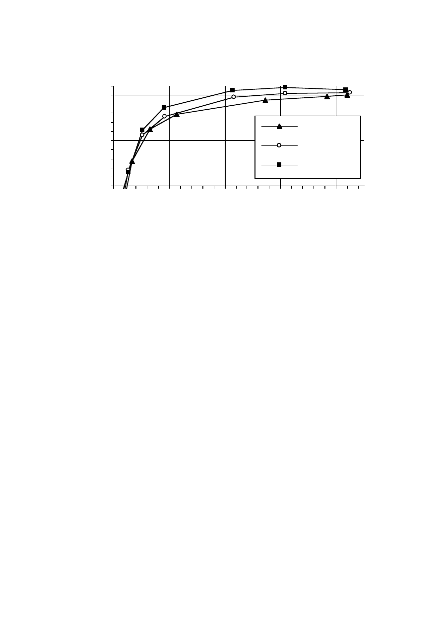
98
Power to the grid (W)
Total efficiency
0,8
0,85
0,9
0
10000
20000
30000
40000
500-1393 rpm
500-1500 rpm
567-1700 rpm
Figure 4.8
The measured maximum efficiency of the 50 kVA generator and
converter system for three different gear ratios.

99
5 Comparison of constant and variable speed
In this chapter the per unit model is used to find the power from different
parts of the wind converter system as functions of wind speed. These
functions are used to see how the losses change with the control strategies.
Constant-speed and two-speed operation of the turbine are compared to
variable speed. For the variable-speed operation two different rated speeds
and two different voltage controls are considered.
By using a wind distribution model the annual energy passing through
different parts of the system can be found. From these annual energy values,
the average efficiency of the gear, the generator and the total mechanical to
electrical power convertion is calculated. Also approximate values of the
difference in energy production between a constant-speed, a two-speed and a
variable-speed turbine are calculated. All these efficiencies and the energy
production are calculated for turbine sites with various median wind speeds,
from 0.35 p.u. to 0.70 p.u.
This comparison is based on equally efficient generators for the variable-
speed and the constant-speed systems. The differences between the
generators in the two systems are that the variable-speed generator has
additional losses and a commutation voltage drop due to the diode rectifier.
5.1 The per unit turbine model
The calculations are made for the 300 kW design example system. For these
calculations only a few of the quantities used in Chapter 3 are needed. The
quantities used are shown in Figure 5.1. The power values are in this chapter
always related to the turbine shaft power at rated operation. This is
important when the parameters for the model are determined, since the
losses of the generator and converter are not in per unit of the rated
generator and converter power. The reason for this is that the total losses
should be the sum of the per unit losses in the different components. Values
of the loss parameters in Chapter 3 are all related to the rated power of the
described component. Now, they will be a little smaller since the losses are
related to a larger power. In Table 5.1 the per unit quantities used in the
calculations are shown. To separate the different control strategies the
indices in Table 5.2 are added to the quantity names.
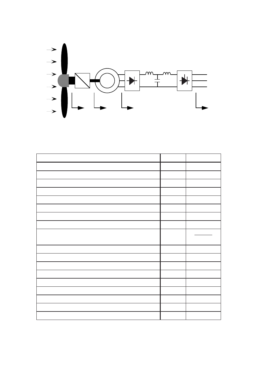
100
n'
t
= n' = n'
g
p
t
p
g
p
a
p
i
v
u
a
Figure 5.1
The quantities used in the per unit calculations in Chapter 5.
Table 5.1
Per unit quantities and constants used in this chapter and the
base values.
Quantity
Notation
Base value
Per unit wind speed
v
v
N
Per unit start wind speed
v
0
v
N
Per unit wind speed of rated power
v
N
v
N
Max operational per unit wind speed
v
max
v
N
Per unit median wind speed
v
m
v
N
Per unit turbine power
p
t
P
t N
Per unit generator speed (= turbine speed)
n'
n
g N
(n
t N
)
Per unit generator mechanical power
p
g
P
t N
Per unit armature voltage
u
a
P
a N
√
3 I
a N
Per unit generator electrical power
p
a
P
t N
Per unit power from the inverter
p
i
Pt N
Per unit power losses
p
loss
Pt N
Power coefficient
C
P
C
P max
Per unit annual energy capture of the turbine
e
t
P
t N
8760 h
*
Per unit annual input energy of the generator
e
g
P
t N
8760 h
*
Per unit annual output energy from the gen.
e
a
P
t N
8760 h
*
Per unit annual output energy from the inverter
e
i
P
t N
8760 h
*
Per unit Weibull probability density
w
—
*) one year is 8760 hours.
101
Table 5.2
The indices used for the constants and functions in this chapter.
Indices
Notation
Constant speed
CS
Two speeds
TS
Low speed (of two)
TS1
High speed (of two)
TS2
Variable speed
VS
Variable speed, 1.2 p.u. rated speed
VS12
Optimum voltage control
VSopt
Optimum voltage control with 1.2 p.u. as rated speed
VSopt12
5.2 Power and losses as functions of the wind speed
5.2.1 Assumptions for the power functions
It is assumed that the wind turbine generator system is designed for a
certain mechanical power from the wind turbine. When comparing the
constant-speed system with the variable-speed system, the maximum input
power from the turbine is the same but not the output power to the grid. The
variable-speed system thus has a little lower rated electric power than the
constant-speed system due to increased generator losses and the converter
losses. The rated generator input power is, however, the same in both the
constant-speed system and the variable-speed system because the gear
losses at rated power are equal for both systems.
To be able to find the difference between a variable-speed and a constant-
speed system, without including the different efficiency of different generator
types, it is assumed that the generator used in the constant-speed system is
the same as the one used in the variable-speed system. However, since the
variable-speed generator is connected to a frequency converter, it has higher
losses compared with the network-connected generator. The voltage drop of
the variable-speed generator is also higher due to the diode commutations.
The efficiency of the two-speed generator is based on efficiency data for a 250
kW/75 kW 4/6-pole ABB induction generator and not on the loss model. That
loss data have been modified to be comparable to the losses of the 300 kW
design example generator. When compared with generators of the same size
but with only one speed the efficiency is roughly 1 % lower for a two-speed

102
generator. Such a difference is included in this comparison as a 0.7 % lower
efficiency at rated power for the two-speed generator than for the constant-
speed generator.
Since all functions will be expressed with the wind speed as a parameter, the
turbine speed as a function of the wind speed must be defined. That is simple
for the cases considered in this report. Either the wind turbine runs at
constant speed with a rated speed of 1 p.u. and a low speed for the two-speed
generator equal to 2/3 p.u. or variable speed with optimal C
P
control is used
and the tip-speed ratio is kept constant. Hence the turbine speed is
proportional to the wind speed up to the rated wind speed. Above the rated
wind speed the turbine speed is assumed to be kept constant.
n'
CS
= 1
(Speed of the constant-speed generator)
(5.1)
n'
TS1
=
2
3
(Low speed of the two-speed generator)
(5.2)
n'
TS2
= 1
(High speed of the two-speed generator)
(5.3)
n'
VS
(v) = v
(Speed of the variable-speed generator)
(5.4)
n'
VSopt12
(v) = 1.2 v
(Higher variable speed)
(5.5)
The generator is started as soon as the wind speed is high enough for the
turbine to produce more than the total system losses. These include losses in
the gear plus generator and for the variable-speed system also the converter
no-load losses. The start-up wind speed is not the same for the different
control strategies because the losses are different. The start-up wind speed
can for the constant- and two-speed systems be found as the lowest wind
speed for which the generator output power is zero. At a lower wind speed the
no load losses will make the generator power negative. The start-up wind
speed v
0
is found by solving the following equation
p
a
(v
0
) = 0
(5.6)
The two-speed system changes speed at the wind speed for which the higher
speed produces as much power as the lower speed. This wind speed v
0TS2
is
found by solving the following equation

103
p
aTS1
( v
0 TS2
) = p
a TS2
( v
0 TS2
)
(5.7)
For the variable-speed system the start-up wind speed is found as the lowest
wind speed for which the output power of the inverter is zero
p
i
( v
0 VS
) = 0
(5.8)
The rated wind speed of the turbine is here defined as the lowest wind speed
at which the turbine can produce rated power. This wind speed is used as
base quantity for the per unit wind speeds. The rated wind speed of the
complete wind turbine generator system depend on how the turbine speed is
controlled. With the used definition of the rated wind speed the constant-
speed turbine reaches rated power at a wind speed above 1 p.u. The reason
for this is that the gear ratio is chosen to maximize the turbine efficiency at a
wind speed of about 0.7 p.u. to maximize the energy production. The variable-
speed turbine also reaches the rated power at a wind speed slightly higher
than 1 p.u., because it is not assumed possible to keep the turbine perfectly
at its optimum tip-speed ratio.
The rated wind speeds for the different systems, v
N
, are found by solving the
following equation:
p
t
( v
N
) = 1
(5.9)
The turbine is shut down when the wind speed exceeds 1.7 p.u.
v
max
= 1.7 p.u.
(5.10)
The start-up wind speed, rated wind speed and shutdown wind speed for the
different systems are found in Table 5.3.
To be able to use the model the turbine power coefficient as a function of tip-
speed ratio must first be modelled. Data are used for a three-bladed pitch-
controlled 12 m turbine. The approximate turbine C
P
curve is a sixth-order
curve fit and can be seen in Figure 5.2.
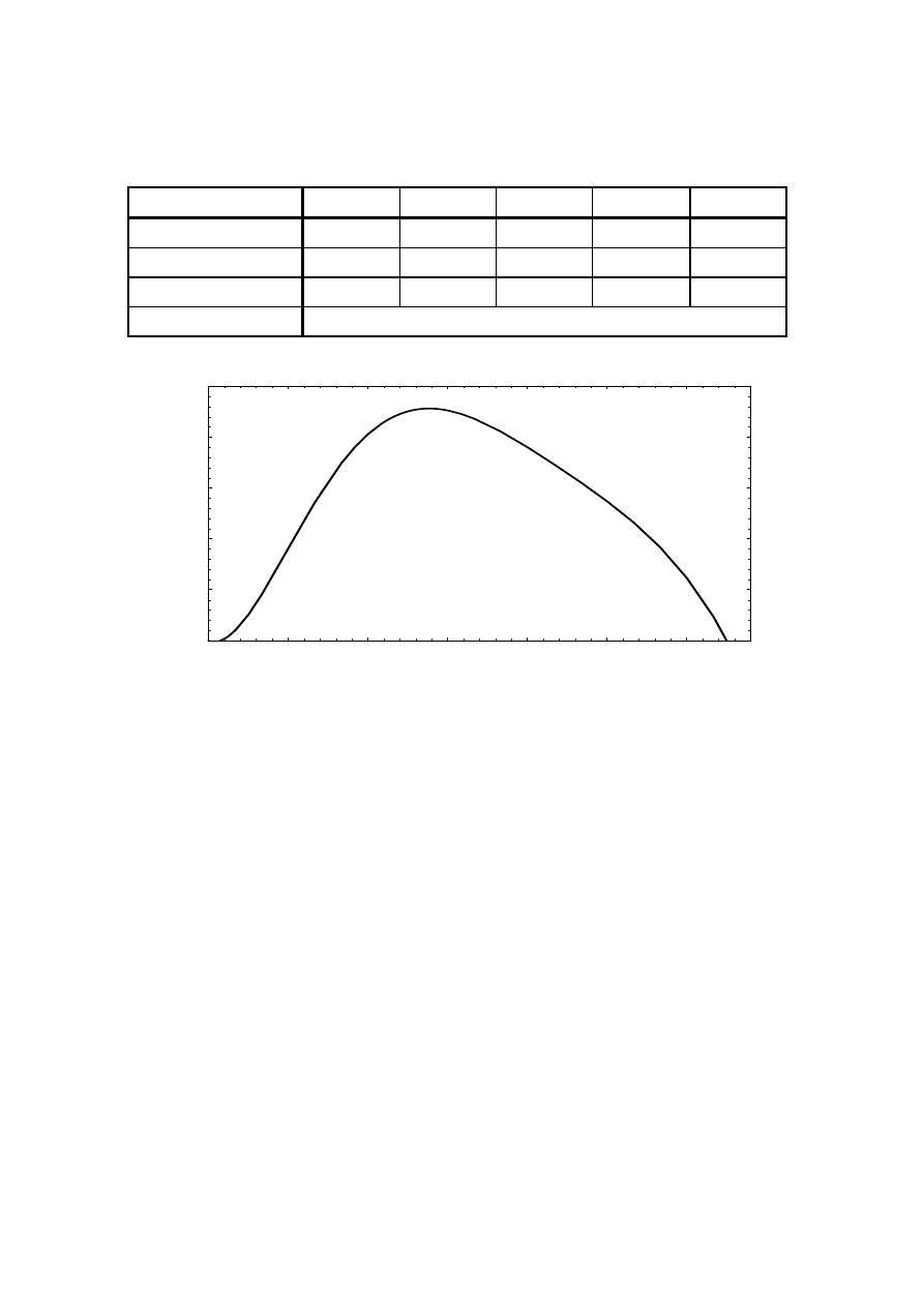
104
Table 5.3
The start-up wind speed, speed-change wind speed, rated wind
speed and shutdown wind speed for different systems.
CS
TS
VS
VSopt
VSopt12
v
0
0.38
0.29
0.20
0.18
0.18
v
0TS2
–
0.62
–
–
–
v
N
1.05
1.05
1.01
1.01
1.01
v
max
1.70
2.5
5
7.5
10
12.5
15
Tip-speed ratio
0
0.1
0.2
0.3
0.4
0.5
Turbine power coefficient
Figure 5.2
Approximation of the power coefficient curve of the turbine.
In the variable-speed system the generator speed is controlled to keep the
turbine power coefficient C
P
at its maximum value for all wind speeds.
However, the turbine speed can not change as fast as the wind speed and,
therefore, the turbine can not keep a constant maximum C
P
. To include this
effect in the calculations without making dynamic simulations the variable-
speed turbine is supposed to maintain an average C
P
a little lower than the
maximum C
P
. A lower average C
P
means a loss of energy production. The
magnitude of this energy loss depends on the control of the turbine. A study of
the optimum control of a wind turbine has been made and it shows that with
a shaft torque variation of about 20 % the mean power loss is only about
2.5 %, [14]. This is only an estimation of the average C
P
but the error of the
estimation does not affect the calculated average efficiencies much. The
accuracy of the calculated energy production is on the other hand directly
affected by the error in average C
P
.

105
5.2.2 Power functions
First the parameters of the gear loss model, the generator loss model and the
converter loss model must be determined. This is done by using the results in
Chapter 3.
Now the turbine energy-capture function, p
t
(v), can be calculated. It is
different for the variable-speed turbine, the two-speed turbine and the
constant-speed turbine. Therefore, different power functions are defined for
the different systems. For the two-speed system two different functions are
used. In the C
P
function the tip-speed ratio,
λ
, is replaced by
λ
=
C n'
v
(5.11)
where C is a constant determined by the rated wind speed v
N
the turbine
diameter d
t
and the rated turbine speed n
t N
. The constant is
C =
n
t N
π
d
t
v
N
(5.12)
The turbine power functions p
t
(v) can now be expressed, below rated power,
as
p
t
(v) = v
3
Cp
C n'(v)
v
(5.13)
where Cp(
λ
) is the approximation of the turbine power coefficient curve.
Then the output power of the gear pg(v) is calculated
p
g
(v) = p
t
(v) – p
loss gear
( p
t
(v) , n'(v) )
(5.14)
where p
loss gear
( p
t
, n' ) is the losses of the gear.
The losses of the generator are defined by the loss model with armature
voltage, armature current and shaft speed as variables. The armature
current is, however, not known yet. Therefore, the generator losses can not
be calculated explicitly. Instead, the output power of the generator is

106
calculated as a function of input power, speed and armature voltage. The
output power p
a
is defined by
p
a
= p
g
– p
loss g
( p
a
/u
a
, u
a
, n' )
(5.15)
where the unknown armature current simply has been replaced by p
a
/u
a
.
p
loss g
is the loss function from the loss model and p
g
is the gear output
power. The result is armature output power as a function of p
g
, u
a
and n'
g
.
Note that the loss parameters for the generator loss function are not the
same for constant-speed operation and variable-speed operation.
Only for the two-speed generator the losses are expressed as explicit
functions because the losses for this generator type are not based on the loss
model but on empirical data for an ABB generator. The loss data are first
adjusted to be comparable to the design example generator, then the loss
functions are obtained as curve fits to the data. The approximate loss
functions of the two speed generator are
p
loss gTS1
(p
g
) = 0.013 + 0.100
p
g
+ 2 p
g
2
3
(5.16)
p
loss gTS2
(p
g
) = 0.026 + 0.033
p
g
+ 2 p
g
2
3
(5.17)
Now the output power of the generator p
a
(v) can be calculated for the three
types of turbine control as well as for two different gear ratios in the variable-
speed system.
The inverter output power p
i
(v) is expressed for three different control
strategies. This function is only used for the variable-speed system, since the
constant-speed and two-speed systems do not have any converter. The
variable-speed generator voltage is either controlled to have a constant flux
or to maximize the generator and converter efficiency. Two gear ratios are
used which gives 1.0 and 1.2 p.u. generator speed at rated power. The
optimum efficiency functions can not be explicitly defined. They are instead
defined as the maximum value of p
i
when u
a
is changed.
Now the harmonics filter losses and the transformer losses can be added to
the loss model. This is, however, not included in this report.
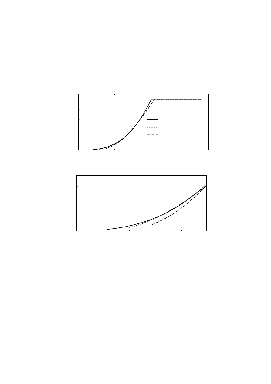
107
5.2.3 Turbine power
The turbine power for the variable-speed turbine, the two-speed and the
constant-speed turbine is calculated for different wind speeds. The power
versus wind speed curves for the design example turbine with constant- or
variable-speed operation is shown in Figure 5.3.
0.5
1
1.5
Wind speed (p.u.)
0
0.2
0.4
0.6
0.8
1
Turbine power (p.u.)
Variable speed
Low speed
High speed
0.1
0.5
0.6
Wind speed (p.u.)
0
0.1
0.2
Turbine power (p.u.)
v
0VS
v
0TS1
v
0CS
Figure 5.3 The power produced by a constant-speed, a two-speed and a
variable-speed turbine. The low wind speed range is enlarged to
show the difference between variable-speed and two-speed
operations.
The power production of the turbine is not much higher for a variable-speed
turbine than for a constant-speed turbine. The difference is that the variable-
speed turbine produces more at low wind speeds. For medium wind speeds the
constant-speed turbine produces just as much as the variable-speed turbine.
Close to rated wind speed the variable-speed turbine produces more and it
reaches rated power at a little lower wind speed than the constant-speed
turbine. By using a two-speed turbine, the power production at low wind
speed is almost equal to that of the variable-speed turbine.
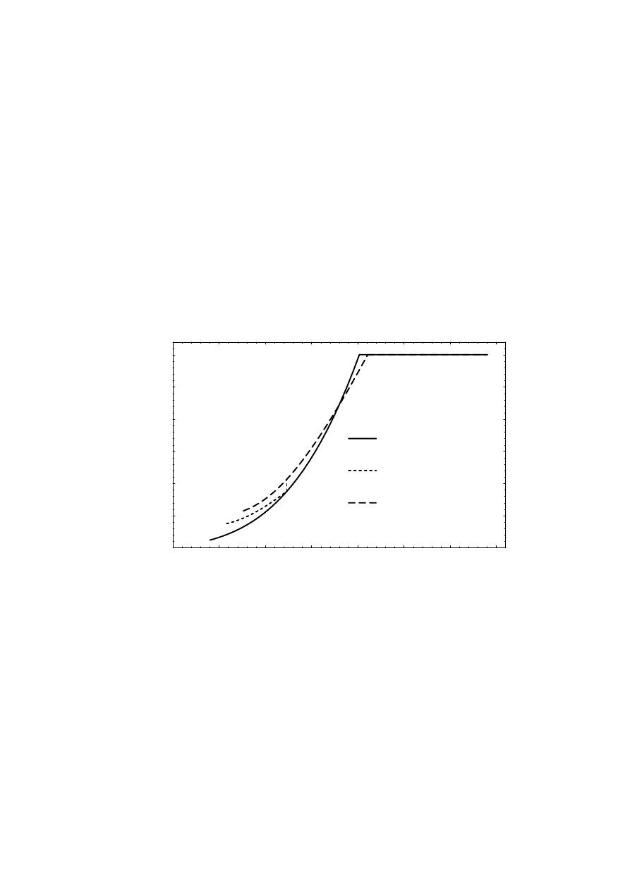
108
5.2.4 Gear losses
The gear losses only depend on the speed of the turbine and the power from
the turbine. They have two parts, the no-load losses which decrease with the
speed of the turbine and the gear mesh losses which are a fixed percentage of
the turbine power. In the constant-speed system the no-load gear losses are
constant, while they are reduced at low speed in the variable speed system.
The gear mesh losses are, for a certain turbine power, the same for all
systems. In the two-speed system the no-load losses are reduced when the
speed is reduced. Figure 5.4 shows the losses of the gear versus wind speed in
the different systems.
0.25
0.5
0.75
1
1.25
1.5
1.75
Wind speed (p.u.)
0
0.005
0.01
0.015
0.02
0.025
0.03
Gear losses (p.u.)
Constant speed
Two speeds
Variable speed
Figure 5.4
The losses of the gear in a constant-speed, two-speed and a
variable-speed wind turbine generator system.
5.2.5 Generator and converter losses
The losses of the constant-speed and two-speed generators are compared
with the losses of the variable-speed generator and converter. The variable-
speed system has a rated speed of 1 p.u. and optimized voltage control.
In Figure 5.5 it can be seen that the variable-speed system has lower losses
than the network-connected constant- and two-speed generators up to about
0.7 p.u. wind speed. The lower total losses are achieved by reducing the no-
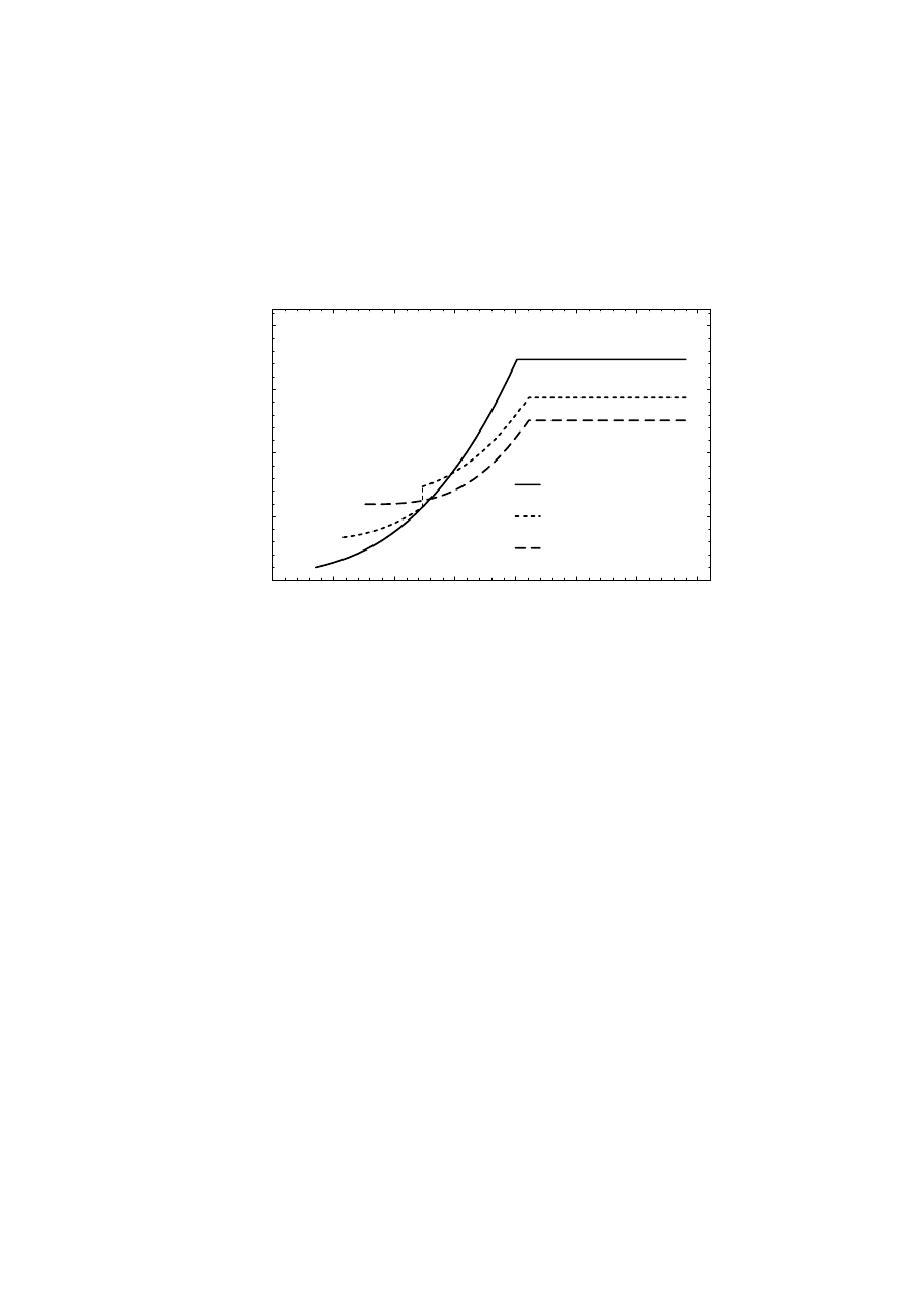
109
load losses of the generator by the voltage control. At high wind speed, the
variable-speed system has higher losses than the network-connected
generators due to the losses in the frequency converter and additional
generator losses.
0.25
0.5
0.75
1
1.25
1.5
1.75
Wind speed (p.u.)
0
0.02
0.04
0.06
0.08
Generator and converter losses (p.u.)
Variable speed
Two speeds
Constant speed
Figure 5.5 The losses of the constant-speed and two-speed generators
compared to the generator and converter losses of the variable-
speed system.
A two-speed generator can not be utilized fully for both speeds and therefore
it has higher losses than the constant-speed generator when it runs on the
high speed. At the low speed the two-speed generator has lower losses
because the friction, windage and core losses are reduced.
5.2.6 Losses at different voltage controls
The variable-speed system can be controlled in different ways. The voltage
control can be used to minimize the losses of the generator and converter.
The effect of such an optimization is shown in Figure 5.6 where the losses of
the generator and converter at constant rated flux and with minimized losses
are compared.
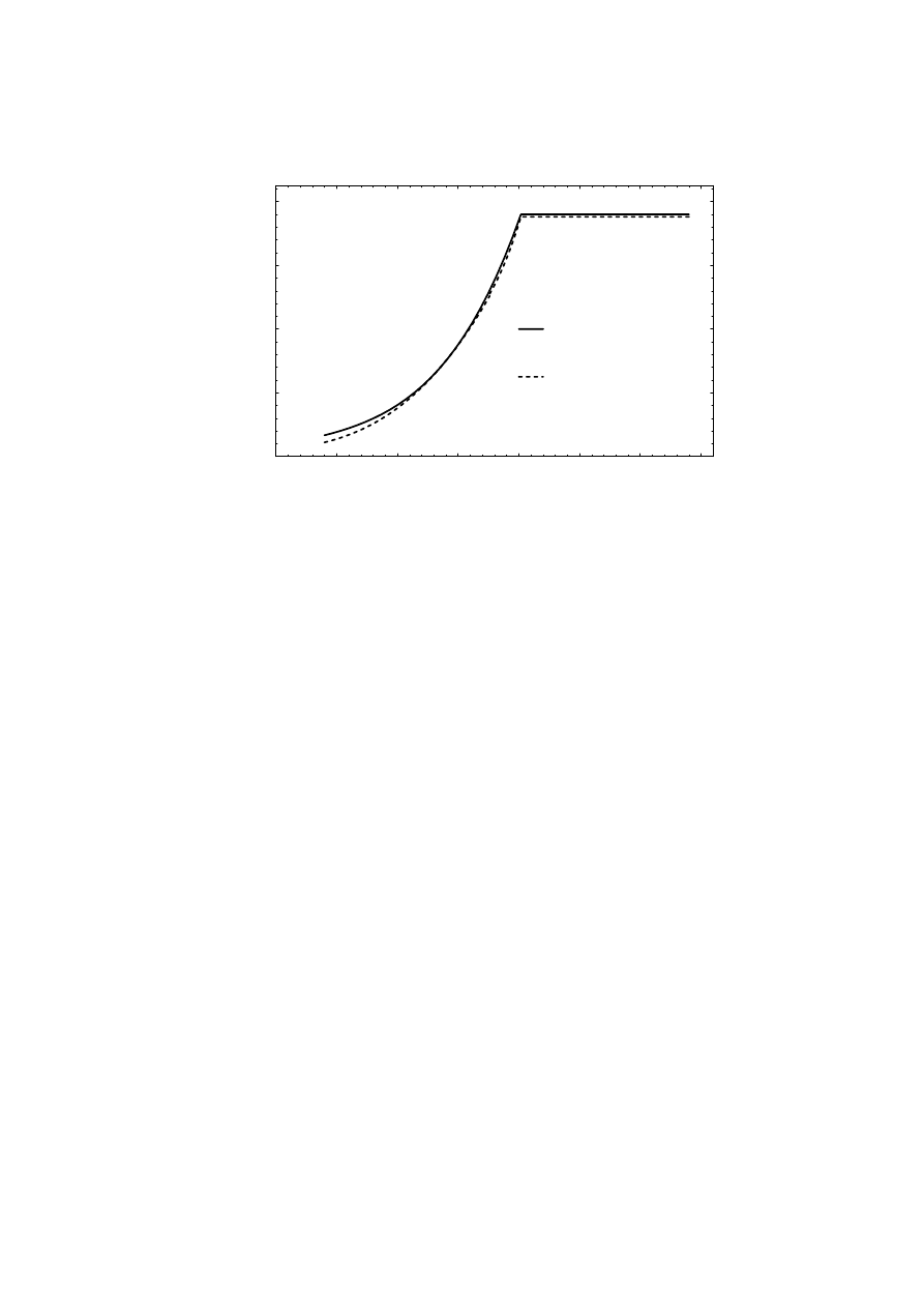
110
0.25
0.5
0.75
1
1.25
1.5
1.75
Wind speed (p.u.)
0
0.02
0.04
0.06
0.08
Generator and converter losses (p.u.)
Constant flux
Optimum flux
Figure 5.6
The losses of the variable-speed generator and converter at
constant rated flux and with minimized losses.
In Figure 5.6 the difference in losses in the variable-speed generator and
converter system can be seen. If the flux is kept constant at its rated value
the losses are unnecessarily high. By optimizing the flux, the losses at low
loads are reduced because of reduced core losses. At rated power the
optimized flux is a little higher than rated flux leading to a higher voltage, and
thus the copper losses are reduced. The losses are reduced by raising the
speed, but the difference between normal rated speed and 20 % higher speed
is small and can not be clearly seen in this type of diagram.
5.2.7 Produced electric power
The electric power versus wind speed is shown in Figure 5.7. The power
production of the variable-speed and two-speed systems is higher than the
production of the constant-speed system at low wind speeds. At medium wind
speed the constant-speed system produces a little more because of the lower
losses and because the variable-speed turbine can not keep the tip-speed
ratio perfectly. Close to the rated wind speed, the variable-speed turbine
produces more, and it also reaches the rated power at a lower wind speed
than the constant-speed turbine does. Above the rated wind speed, the
constant-speed system produces more because it has lower losses. The
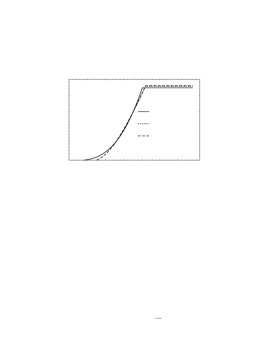
111
difference between the constant-speed and two-speed systems can only be
seen at low wind speed. The two-speed system has a lower start-up wind
speed than the constant-speed system and the produced power is higher up
to the speed-change wind speed.
0.25
0.5
0.75
1
1.25
1.5
1.75
Wind speed (p.u.)
0
0.2
0.4
0.6
0.8
1
Electric output power (p.u.)
Variable speed
Two speeds
Constant speed
Figure 5.7
The electric power produced by a constant-speed turbine, two-
speed turbine and a variable-speed turbine.
5.3 Energy and average efficiency
From the above presented power outputs at different wind speeds an annual
energy can be calculated. This is done by integrating the power, from the
start-up wind speed to the shutdown wind speed, with the wind speed
probability function as a weighting function. A Weibull distribution of wind
speeds is assumed when the weighting function is derived, see Figure 5.8. The
integral of the weigthing function over all wind speeds from zero to infinity is
by definition equal to 1. The Weibull distribution is the usual way to specify
the wind resources for different turbine sites. The distribution has two
parameters, here the median wind speed v
m
and a shape factor c. For normal
wind distribution c is about 2, which is assumed here. The Weibull probability
distribution is defined as
w(v,c,v
m
) = v
m
-c
Log(2) c v
(c-1)
e
-Log(2)
v
v
m
c
(5.18)
112
0.25
0.5
0.75
1
1.25
1.5
1.75
(p.u.)
Weighting function
(Weibull distribution, c=2)
0
0.5
1
1.5
2
2.5
= 0.35 p.u.
= 0.50 p.u.
= 0.70 p.u.
v
v
v
v
m
m
m
Figure 5.8
The weighting functions for three different median wind speeds.
In Figure 5.9 the energy density function shown. It is the product of the
power and the weighting function. The integral of energy density function,
from zero wind speed to the shutdown wind speed, is the annual energy in per
unit.
In the energy density diagram it can be seen that the energy production at
wind speeds just below rated wind speed gives the most important
contribution to the total energy production. The energy production above
rated wind speed is not as important because the probability of so high wind
speeds is low. Contrary to what can be guessed from the power versus wind
speed function the energy production at low wind speed is not negligible. The
power is low at low wind speeds but the probability of these wind speeds is
high making the contribution to the energy production significant.
5.3.1 Assumptions for the energy calculations
The main objective of the comparison between variable-speed and constant-
speed systems is to find the average energy conversion efficiency. As a step
in the calculation of the average efficiency the energy production is also
calculated. Average efficiency is here defined as the output energy divided by
the input energy. Since the calculation is made in per unit the calculated
energy production is by definition the same as the average power production
because the energy is calculated for a time equal to 1 p.u.
113
Since the Weibull distribution parameters are derived from 10 minutes
average wind speeds, the result of the energy calculations has errors,
especially for the variable-speed system. However, the error of the output
energy is almost the same as the error of the input energy. Since the
efficiency is the quotient of output and input energy, this error is small in the
efficiency values.
Power(wind speed)
Weighting function(wind speed)
Area = 1
Energy density(wind speed)
Area
=
Energy
Figure 5.9
The energy density function, equal to the power times the
weighting function.
The energy integrations are made for sites with different median wind speeds,
between 4.55 m/s and 9.1 m/s. The rated wind speed of the turbine is here
assumed to be 13 m/s and the median wind speeds considered are then from

114
0.35 to 0.7 p.u. At low wind speed sites the median wind speed is in the range
0.35 to 0.45 p.u. (4.55 to 5.85 m/s). Wind turbine generator systems are
usually not located at these sites. If the median wind speed is in the range
0.45 to 0.55 p.u. (5.85 to 7.15 m/s) the site is a normal wind speed site and
most wind turbine generator systems are located at these sites. Sites of a
median wind speed between 0.55 and 0.70 p.u. (7.15 to 9.1 m/s) is high wind
speed sites and they are rarely found in Sweden.
5.3.2 Wind energy captured by the turbine
The turbine energy capture is calculated first by integrating the turbine
power functions P
t
(v) multiplied by the weighting function from the system
start-up wind speed to the rated wind speed. Then the rated power multiplied
by the total probability of wind speed between rated wind speed and the
shutdown wind speed is added. The result from this calculation is the per unit
energy captured by the turbine during a year with the chosen wind speed
probability curve. The wind speeds for start-up, rated power and shutdown of
the turbine are v
0
, v
N
and v
max
. The energy captured by the turbine is defined
as
e
t
(c,v
m
) =
∫
v
0
v
N
w(v,c,v
m
) p
t
(v) dv + p
t
(v
N
)
∫
v
N
v
max
w(v,c,v
m
) dv (5.19)
5.3.3 Gear energy output and average gear efficiency
The per unit energy output from the gear is defined in the same way as the
turbine energy
e
g
(c,v
m
) =
∫
v
0
v
N
w(v,c,v
m
) p
g
(v) dv + p
g
(v
N
)
∫
v
N
v
max
w(v,c,v
m
) dv (5.20)
The energy from the gear can, together with the turbine energy, be used to
calculate the average efficiency of the gear. The average gear efficiency for a
site with the median wind speed v
m
can be found as
η
gear
=
e
g
(c,v
m
)
e
t
(c,v
m
)
(5.21)
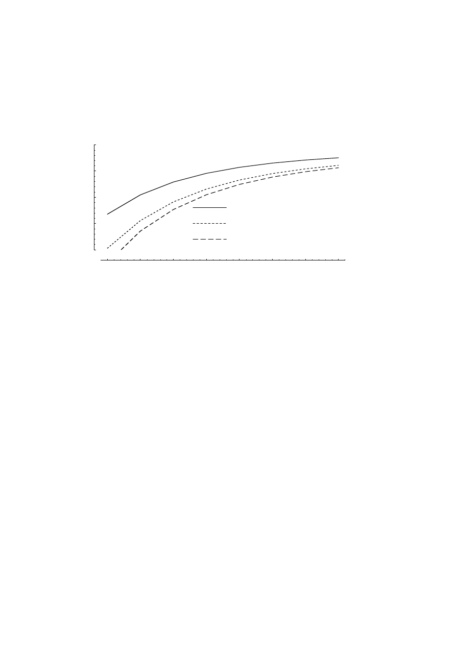
115
The average gear efficiency is calculated for different median wind speeds
from 0.35 to 0.7 p.u. and plotted in Figure 5.10.
0.35
0.4
0.45
0.5
0.55
0.6
0.65
0.7
(p.u.)
Average efficiency of the gear
0.95
0.955
0.96
0.965
0.97
Variable speed
Two speeds
Constant speed
m
v
Figure 5.10 The average efficiency of the gear in a variable-speed, a two-speed
and a constant-speed turbine.
The average gear efficiency is always higher in a variable-speed system than
in a constant-speed system. This is obvious since the gear losses in a
variable speed system are never higher than in a constant speed system at
equal power. The difference in average efficiency is not large, only 0.2 % for
high wind speed sites, 0.4 % for medium wind speed sites and about 0.7 % for
low wind speed sites. It is a small, but clear, advantage of the variable-speed
wind turbine generator system.
5.3.4 Electric energy and average electric efficiency
In this section the average efficiency of the generator of the constant-speed
system is compared with the average efficiency of the generator and
converter of the variable-speed system. Later in Section 5.3.5 the total
efficiency, including the gear, is presented. The per unit output electrical
energy of the constant-speed generator can be calculated as
e
aCS
(c,v
m
) =
∫
v
0CS
v
NCS
w(v,c,v
m
) p
aCS
(v) dv + p
aCS
(v
N
)
∫
v
NCS
v
max
w(v,c,v
m
) dv
(5.22)

116
For the two-speed system the integration is divided into three parts
e
aTS
(c,v
m
) =
∫
v
0TS1
v
0TS2
w(v,c,v
m
) p
aTS1
(v) dv +
∫
v
0TS2
v
NTS
w(v,c,v
m
) p
aTS2
(v) dv +
+ p
aTS2
(v
NTS
)
∫
v
NTS
v
max
w(v,c,v
m
) dv
(5.23)
For the constant-flux variable-speed system the output energy is the energy
from the inverter
e
iVS
(c,v
m
) =
∫
v
0VS
v
NVS
w(v,c,v
m
) p
iVS
(v) dv + p
iVS
(v
NVS
)
∫
v
NVS
v
max
w(v,c,v
m
) dv
(5.24)
The energy produced when optimized flux and a higher speed is used is
calculated in a similar way.
The average efficiency of the generator system can be calculated by dividing
the output electrical energy by the input mechanical energy from the gear. A
comparison of the average efficiency of the generator system is made to find
how efficient a variable-speed generator system is compared to a constant-
speed system. First the variable-speed system with optimized efficiency is
compared with a two-speed system and a constant-speed system.
It is found, from Figure 5.11, that the optimized variable-speed system often
is about as efficient as the constant-speed system in converting the
mechanical energy of the generator shaft into electric energy to the grid. On
sites with low median wind speed the variable-speed system is more efficient
because of its low losses at low power. The efficiency is a little lower or as
high as the efficiency of a constant-speed system for normal wind speed sites.
For high wind speed sites the variable-speed generator system is always less
efficient. The average efficiency of the two-speed system is rather similar to
the one of the constant-speed system. It is a little lower at high wind speed
sites and a little higher at low wind speed sites.
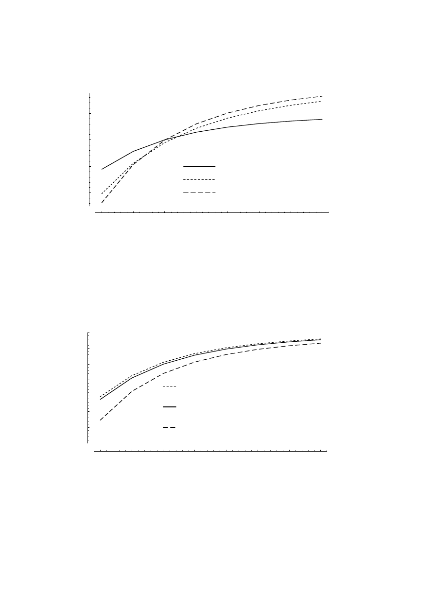
117
0.35
0.4
0.45
0.5
0.55
0.6
0.65
0.7
(p.u.)
Average efficiency of generator (and converter)
0.86
0.88
0.9
0.92
Variable speed
Two speeds
Constant speed
m
v
Figure 5.11 Average electric efficiency of a two-speed, a constant-speed system
and a variable-speed system using optimized flux and 1.0 p.u.
rated speed.
The difference in average efficiency between an optimized voltage control and
the often used constant flux voltage control can be seen in Figure 5.12.
0.35
0.4
0.45
0.5
0.55
0.6
0.65
0.7
(p.u.)
Average efficiency of generator and converter
0.86
0.87
0.88
0.89
0.9
0.91
0.92
Optimum voltage n = 0 - 1 p.u.
Constant flux n = 0 - 1 p.u.
Optimum voltage n = 0 - 1.2 p.u.
m
v
Figure 5.12 The average efficiency of a variable-speed system with constant
flux or optimized efficiency and either a rated speed of 1 p.u. or
1.2 p.u.
If optimized voltage control is used instead of constant rated flux the
efficiency will be about 0.5 to 0.8 % higher on sites with normal median wind
speed. On sites with low wind speed the difference in efficiency, between
optimized voltage control and constant flux, can be up to more than 1 %. If a
higher generator speed is used than the speed at 50 Hz, the average
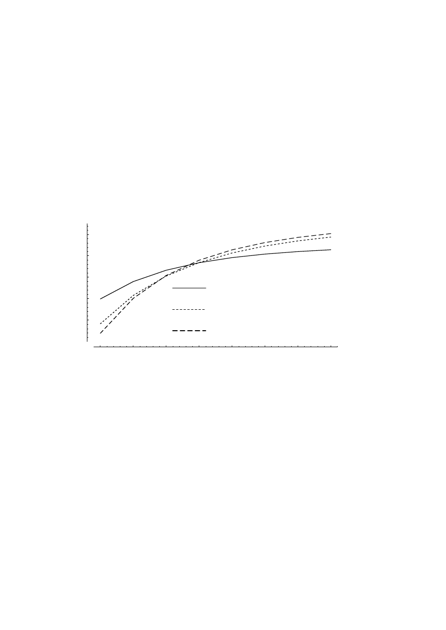
118
efficiency will also improve. The increase in efficiency by using a higher speed
is small, less than 0.2 % for all median wind speeds.
5.3.5 Total efficiency including the gear
To find the average efficiency in converting the turbine shaft energy into
electrical energy, the output electrical energy is divided by the turbine energy.
In Figure 5.13 the resulting average efficiency can be seen. The turbine
efficiency is not included in these figures.
0.35
0.4
0.45
0.5
0.55
0.6
0.65
0.7
(p.u.)
Average efficiency of gear, generator (and converter)
0.82
0.84
0.86
0.88
0.9
Variable speed
Two speeds
Constant speed
v
m
Figure 5.13 The total efficiency in converting the turbine energy into electric
energy fed to the network.
The result is similar to the average efficiency of only the generator and
converter. The only difference is that the gear losses make the constant-
speed system less efficient compared with the variable-speed system.
The laboratory system has a low converter efficiency (95.6 %) compared with
the design example system (98 %). This difference is found to be very
important when a constant-speed and the corresponding variable-speed
system are compared, see Figure 5.14. The lower converter efficiency makes
the average efficiency of the variable-speed system lower than the average
efficiency of the constant-speed system for all median wind speeds. This
shows that an efficient converter is very important if the variable-speed
system shall be as efficient as the constant-speed system.
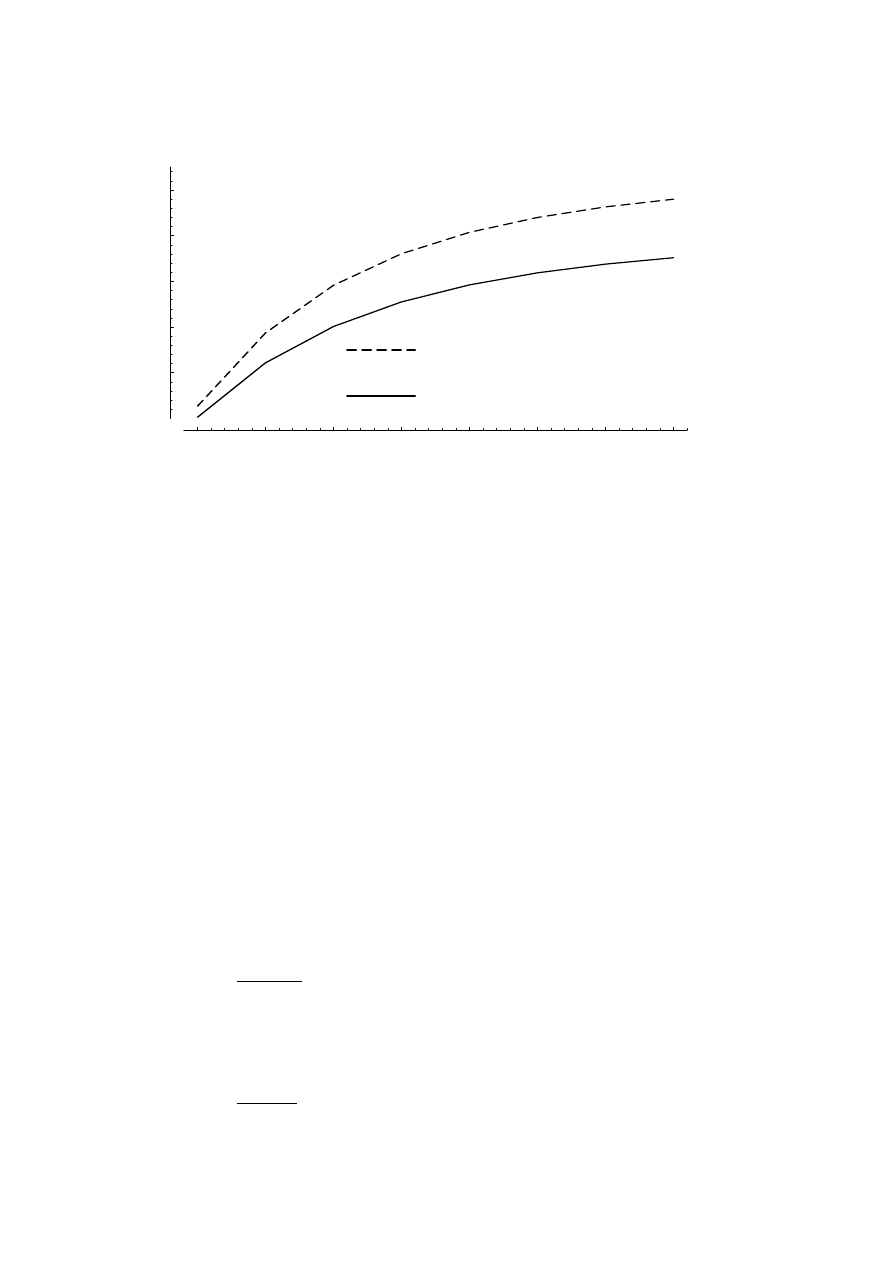
119
0.35
0.4
0.45
0.5
0.55
0.6
0.65
0.7
(p.u.)
Average efficiency of gearbox, generator (and converter)
0.82
0.84
0.86
0.88
0.9
Variable speed
Constant speed
v m
Figure 5.14 Calculated average electric efficiency of the 50 kVA generator
system at constant speed and at variable speed, using optimized
flux and 1.0 p.u. rated speed.
5.3.6 Produced energy
When the average efficiencies are calculated, there are also automatically
results showing the difference in produced electric energy. The calculation
method have been derived for constant-speed turbines and, therefore, the
accuracy of this comparison depends on how accurate the energy calculation
method is for variable-speed turbines. Because of this uncertainty, the
predicted difference must be seen only as a hint of what the real difference
may be.
The capacity factor is defined as the average power production divided by the
rated electric power. In per unit the average electric power is equal to the
produced electric energy. Therefore, the capacity factor C
cap
for the
constant-speed and two-speed systems can be defined as
C
cap
=
e
a
(c,v
m
)
p
a
(v
N
)
(5.25)
For the variable-speed system the capacity factor is defined as
C
cap
=
e
i
(c,v
m
)
p
i
(v
N
)
(5.26)
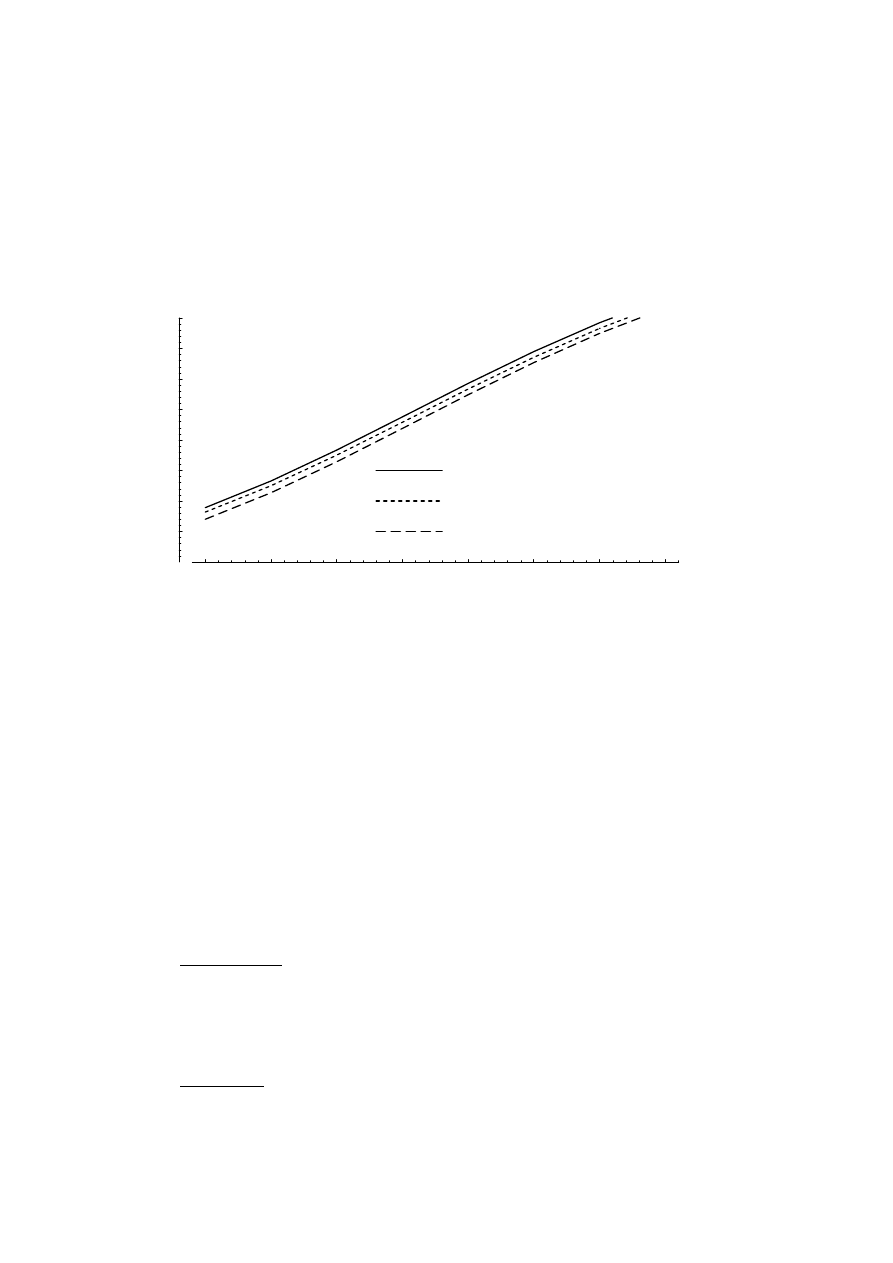
120
The capacity factor of the turbine can be calculated for different control
strategies. The comparison is made for a constant-speed , a two-speed and a
variable-speed wind turbine generator system using optimized flux and a
rated generator speed of 1 p.u. The results are shown in figure 5.15.
0.35
0.4
0.45
0.5
0.55
0.6
0.65
0.7
(p.u.)
Capacity factor
0.05
0.1
0.15
0.2
0.25
0.3
0.35
0.4
Variable speed
Two speeds
Constant speed
m
v
Figure 5.15 The capacity factor of a wind turbine generator system at
constant-speed, two-speed and variable-speed operation.
It can be seen that the capacity factor of the variable-speed system is higher
than that of the constant-speed system. The two-speed system also has a
high capacity factor compared with the constant-speed system. The figure
shows the absolute energy capture, expressed as the capacity factor for
different systems. It is, however, difficult to find the relative increase in the
energy production when a constant-speed system is changed to an equal two-
speed or variable-speed system from Figure 5.15. The relative increase in
production is shown in Figure 5.16. The increase in energy production has
been calculated for the variable-speed system as
e
iVSopt
(c,v
m
)
e
aCS
(c,v
m
)
(5.27)
and for the two-speed system
e
aTS
(c,v
m
)
e
aCS
(c,v
m
)
(5.28)
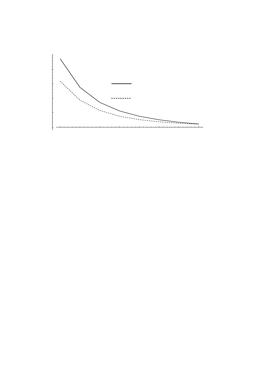
121
0.35
0.4
0.45
0.5
0.55
0.6
0.65
0.7
(p.u.)
Power production compared with a constant-speed system
1
1.05
1.1
1.15
1.2
1.25
Variable-speed system
Two-speed system
m
v
Figure 5.16 The relative increase in produced electric energy if a two-speed or
variable-speed system is used instead of a constant-speed system.
It can be seen that the two-speed system produces more than the constant-
speed system. The difference between two-speed and variable-speed system
is not so large as the difference between constant-speed and two-speed
systems. For a normal median wind speed the increase in energy production
is about 5.2 % if a variable-speed system is used instead of a constant-speed
system. If a two-speed system is used the increase is 3.8 %. This comparison
is made for systems with equal rated turbine power and unequal rated output
power.
5.4 Summary of average efficiency comparison
Although a variable-speed system has extra losses in the generator and
converter it can usually be about as efficient as a constant-speed generator.
At low wind speed sites it is more efficient, at high wind speed sites it is less
efficient. The extra losses in the frequency converter have often been said to
be a disadvantage of the variable-speed system. However, the calculations in
this chapter show that the decrease in generator and gear losses can
compensate for the increase in losses due to the frequency converter.
The calculations are based on the use of an efficient frequency converter,
with a rated efficiency of 98 %. If a transistorized inverter is used, in order to
reduce the network disturbance, the total efficiency will decrease a few

122
percents. Still, the difference in average efficiency between variable-speed
and constant-speed systems will be small at medium wind speed sites.

123
6. Conclusions
A model of the losses in the generator and converter has been derived and
verified for a 50 kVA generator. The model can be used to predict the shaft
torque of the generator with an error of less than 2 % of the rated torque. This
should be sufficient for the steady-state torque control of a wind turbine. The
model only needs measurements of the generator speed, the dc voltage and
the dc current of the converter. Most of the model parameters are, for normal
generators, available from the manufacturer. The rest of the parameters can
be estimated if the demand on the accuracy is not higher than about 2 %,
otherwise they have to be measured.
The loss model can be used to maximize the generator and converter
efficiency. By changing the generator voltage, the efficiency of the system
can be maximized. If the voltage is controlled to maximize the efficiency, the
generator and converter system is about 0.5 to 0.8 % more efficient, in
average, than if the common constant flux control is used. It has also been
found that a variable-speed generator should use a high speed to increase the
efficiency and decrease the generator size. To use a larger standard generator
than necessary does not normally improve the efficiency.
Earlier, it has often been said that the losses in the frequency converter of a
variable-speed system are a drawback. In this report it is, however, shown
that the total energy losses do not have to increase because of the frequency
converter. The generator and gear losses can be reduced when the converter
is used, and this reduction may be large enough to compensate for the losses
in an efficient converter. This means that the annual average efficiency of a
variable-speed generator system can be as high as that of a constant-speed
system, at least for turbine sites of normal wind speed. At high wind speed
sites the average efficiency is lower and at low wind speed sites it is higher in
the variable-speed system than in the constant-speed system.
The loss model has errors in modelling the additional losses and the core
losses. If the accuracy is critical, the additional losses and the core losses
should be investigated more thoroughly.

124
7. References
1
Ernst, J., Drezahlvariable Windenergieanlage mit Gleichstrom-
zwischenkreis-Umrichter und optimum-suchendem Regler, Germany,
Technische Universität Carolo-Wilhelmina zu Braunschweig,
Dissertation, 1986, 169 p.
2
Hoeijmakers, M.J., On the steady-state performance of a synchronous
machine with converter, The Netherlands, Technical University of
Eindhoven. Dissertation, 1984, 204 p.
3
Hoeijmakers, M. J., Synchronous machine with rectifier for wind
turbines, IEA 21th meeting of experts – Electrical systems for wind
turbines with constant and variable speed, Göteborg, Sweden, October
7-8, Project Management for Biology, Energy, Ecology (BEO) Research
Centre Jülich (KFA), 1991, p. 51-61.
4
Carlson, O., Analys av synkrongenerator med frekvensomriktare för
elgeneraring vid variabelt varvtal, Göteborg, Sweden, Chalmers
University of Technology, Dept. of Electrical Machines and Power
Electronics, Dissertation, Technical Report No. 185, 1988.
5
Svensson, J., Grauers, A., Carlson, O., Förstudie av elsystem till
vindkraftverk med variabelt varvtal, Göteborg, Sweden, Chalmers
University of Technology, Dept. of Electrical Machines and Power
Electronics, Technical Report No. R-93-07, 1993, 58 p.
6
Ekström, Å., High power electronics, HVDC and SVC, Stockholm,
Sweden, EKC – Electric Power Research Center, The Royal institute of
Technology, 1990.
7
Hoeijmakers, M.J., The (In)stability of a synchronous machine with
diode rectifier, Internatinal Conference on Electrical Machines
(ICEM'92), Manchester, Great Britain, 15 - 17 September 1992,
Proceedings, p. 83–87.
8
Jain, G.C., Design, Operation and Testing of Synchronous Machines,
New York, USA, Asia, 1966, 676 p.

125
9
El-Bakry, M., Wahsh, S., Upper and lower limits in eddy current and
hysteris losses, Internatinal Conference on Electrical Machines
(ICEM'92), Manchester, Great Britain, 15 - 17 September 1992,
Proceedings, p. 1211–1215.
10
Adkins, B., Harley, R.G., The general theory of alternating current
machines, London, Great Britain, Chapman and Hall, 1975, 279 p.
11
Shipley, E.E., Loaded gears in action, In: Dudley, D.W. ed., Dudley's
Gear Handbook, 2nd edition, New York, Townsend, 1991, p. 12.1 to
12.39 .
12
Generator data for the LSA 47 series synchronous generators, France,
Leroy Somer ®, 1992, 6 p.
13
IEC Standard 34-1, Rotating electrical machines, Part 1: Rating and
performance, 8th edition, 1983.
14
Ekelund, T., Schmidtbauer, B., Linear quadratic control of variable
speed wind turbines below rated power, Göteborg, Sweden, Chalmers
University of Technology, Control Engineering Laboratory, Report No.
R 92-04, 1992, 36 p.
Wyszukiwarka
Podobne podstrony:
[US 2005] 6864611 Synchronous generator for service in wind power plants, as well as a wind power
(WinD Power) Dynamic Modeling of Ge 1 5 And 3 6 Wind Turbine Generator {}[2003}
[2006] Analysis of a Novel Transverse Flux Generator in direct driven wind turbine
ANALYSIS OF CONTROL STRATEGIES OF A FULL CONVERTER IN A DIRECT DRIVE WIND TURBINE
Boost Converter Design For 20Kw Wind Turbine Generator
Synchronous generator for service in wind power plants as well as a wind power plant
DIN 61400 21 (2002) [Wind turbine generator systems] [Part 21 Measurement and assessment of power qu
[Engineering] Electrical Power and Energy Systems 1999 21 Dynamics Of Diesel And Wind Turbine Gene
CEI 61400 22 Wind turbine generator systems Required Design Documentation
Ouellette J Science and Art Converge in Concert Hall Acoustics
[2006] Application of Magnetic Energy Recovery Switch (MERS) to Improve Output Power of Wind Turbine
Darrieus Wind Turbine Design, Construction And Testing
20060028025 Wind Turbine Generator System
Blade sections for wind turbine and tidal current turbine applications—current status and future cha
Innovative Solutions In Power Electronics For Variable Speed Wind Turbines
Modeling Of The Wind Turbine With A Doubly Fed Induction Generator For Grid Integration Studies
więcej podobnych podstron