
GE-Power Systems Energy Consulting
Copyright 2002 General Electric Company, U.S.A.
Dynamic Modeling of GE 1.5 and
3.6 Wind Turbine-Generators
Prepared by:
Nicholas W. Miller
William W. Price
Juan J. Sanchez-Gasca
October 27, 2003
Version 3.0
GE
Power
Systems

GE-Power Systems Energy Consulting
Copyright 2002 General Electric Company, U.S.A.
GE WTG Modeling-v3-0.doc, 10/27/03
Foreword
This document was prepared by General Electric International, Inc. through its Power
Systems Energy Consulting (PSEC) in Schenectady, NY.
Technical and commercial questions and any correspondence concerning this document
should be referred to:
Nicholas W. Miller
Power Systems Energy Consulting
General Electric International, Inc.
Building 2, Room 605
Schenectady, New York 12345
Phone: (518) 385-9865
Fax: (518) 385-5703
E-mail: nicholas.miller@ps.ge.com

GE-Power Systems Energy Consulting
Copyright 2002 General Electric Company, U.S.A.
GE WTG Modeling-v3-0.doc, 10/27/03
Legal Notice
This report was prepared by General Electric International, Inc.’s Power Systems Energy
Consulting (PSEC) as an account of work sponsored by GE Wind Energy (GEWE).
Neither GEWE nor PSEC, nor any person acting on behalf of either:
1.
Makes any warranty or representation, expressed or implied, with respect to the
use of any information contained in this report, or that the use of any information,
apparatus, method, or process disclosed in the report may not infringe privately
owned rights.
2.
Assumes any liabilities with respect to the use of or for damage resulting from the
use of any information, apparatus, method, or process disclosed in this report.

GE-Power Systems Energy Consulting
Copyright 2002 General Electric Company, U.S.A.
GE WTG Modeling-v3-0.doc, 10/27/03
Table of Contents
1.
INTRODUCTION ............................................................................................................................1.1
2.
MODEL OVERVIEW AND PHILOSOPHY ................................................................................2.1
2.1
F
UNDAMENTALS
........................................................................................................................2.1
2.2
O
VERALL
M
ODEL
S
TRUCTURE
..................................................................................................2.2
3.
MODELING FOR LOADFLOW ...................................................................................................3.1
3.1
I
NITIAL CONDITIONS FOR DYNAMIC SIMULATION
.......................................................................3.2
4.
DYNAMIC MODEL ........................................................................................................................4.1
4.1
G
ENERATOR
/C
ONVERTER
M
ODEL
.............................................................................................4.1
4.2
E
XCITATION
(C
ONVERTER
) C
ONTROL
M
ODEL
..........................................................................4.3
4.3
W
IND
T
URBINE
& T
URBINE
C
ONTROL
M
ODEL
..........................................................................4.7
4.3.1
Rotor Mechanical Model......................................................................................................4.8
4.3.2
Turbine Control Model.......................................................................................................4.11
4.3.3
Wind Power Model.............................................................................................................4.13
4.4
W
IND
S
PEED
............................................................................................................................4.15
5.
SAMPLE SIMULATION RESULTS .............................................................................................5.1
5.1
C
OMPARISON WITH
M
EASURED
D
ATA
.......................................................................................5.1
5.2
R
ESPONSE TO
F
AULT
.................................................................................................................5.2
5.3
R
ESPONSE TO
W
IND
S
TEP
..........................................................................................................5.4
6.
OTHER TECHNICAL ISSUES ......................................................................................................6.1
6.1
E
QUIVALENCING
........................................................................................................................6.1
6.2
A
PPLICABILITY OF
M
ODEL TO
O
THER
WTG
S
............................................................................6.1
7.
CONCLUSIONS...............................................................................................................................7.1

GE-Power Systems Energy Consulting
Copyright 2002 General Electric Company, U.S.A.
1.1
GE WTG Modeling-v3-0.doc, 10/27/03
1. Introduction
GE Power Systems Energy Consulting has an ongoing effort dedicated to development of
models of GE wind turbine generators (WTG) suitable for use in system impact studies.
This report documents the present recommendations for dynamic modeling of the GE 1.5
and 3.6 WTG for use in studies related to the integration of GE wind turbines into power
grids. This report includes recommended model structure and data, as well the
assumptions, capabilities and limitations of the resulting model.
The model provided is as simple as is appropriate for bulk power system dynamic
studies. It is valuable to put the model limitations in the context of what analysis is
required. First and most important, this model is for positive sequence phasor time-
domain simulations – e.g. PSLF or PSS/e. Second, this assumes that the analysis is
mainly focused on how the WTGs react to grid disturbances, e.g. faults, on the
transmission system. Third, the model provides for calculation of the effect of wind
speed fluctuation on the electrical output of the WTG. Details of the device dynamics
have been substantially simplified. Specifically, the very fast dynamics associated with
the control of the generator converter have been modeled as algebraic (i.e. instantaneous)
approximations of their response. Representation of the turbine mechanical controls has
been simplified as well. The model is not intended for use in short circuit studies.
GE-Power Systems Energy Consulting
Copyright 2002 General Electric Company, U.S.A.
2.1
GE WTG Modeling-v3-0.doc, 10/27/03
2. Model Overview and Philosophy
2.1 Fundamentals
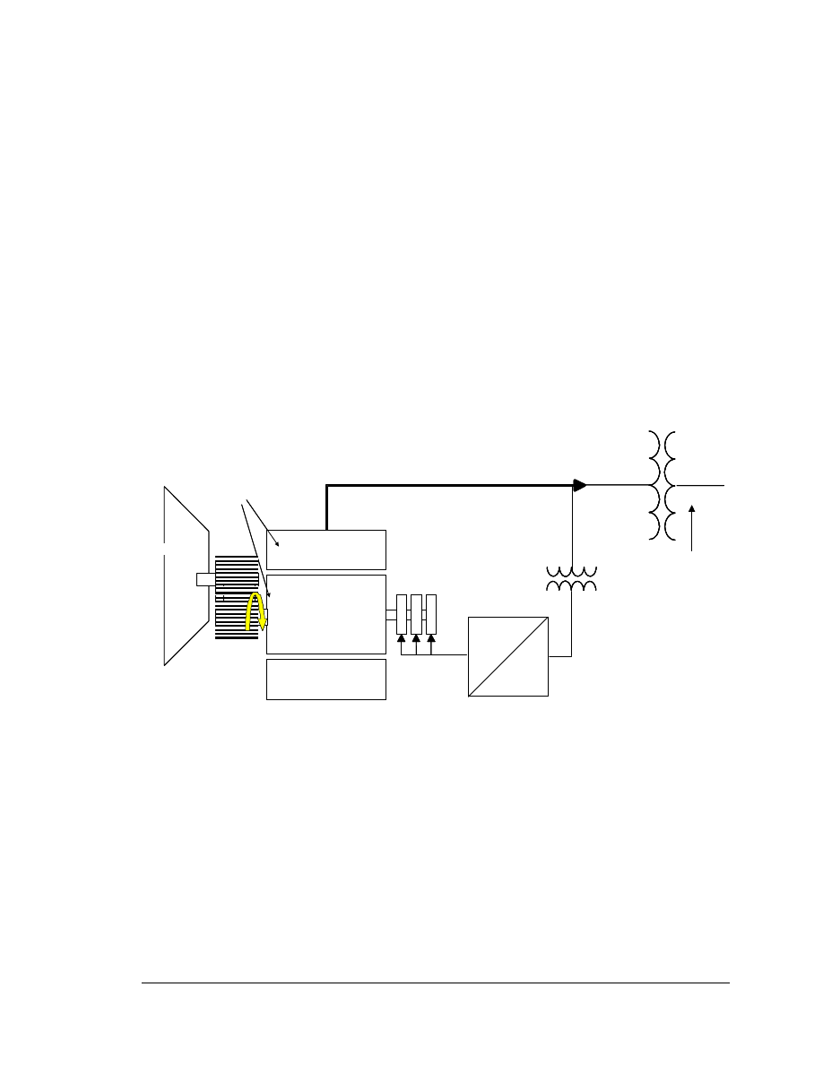
A simple schematic of an individual GE Wind Turbine-Generator (WTG) is shown in
Figure 2-1.
The GE WTG generator is unusual from a system simulation perspective. Physically, the
machine is a relatively conventional wound rotor induction (WRI) machine. However,
the key distinction is that this machine is equipped with a solid-state voltage-source
converter AC excitation system. The AC excitation is supplied through an ac-dc-ac
converter. For the GE 3.6 machine the converter is connected as shown. For the GE 1.5
machine it is connected directly at the stator winding voltage. Machines of this structure
are termed ‘double fed’, and have significantly different dynamic behavior than either
conventional synchronous or induction machines. Modeling of the GE 1.5 and 3.6
machines with conventional dynamic models for either synchronous or induction
machines is, at best, highly approximate and should be avoided.
Wind Turbine
f
rotor
P
rotor
f
net
P
stator
f
rotor
P
rotor
f
net
P
conv
3
φ
AC Windings
Field Converter
f
net
P
net
Q
net
Collector System
(e.g. 34.5kV bus)
Wind Turbine
f
rotor
P
rotor
f
net
P
stator
f
rotor
P
rotor
f
rotor
P
rotor
f
net
P
conv
P
conv
3
φ
AC Windings
Field Converter
f
net
P
net
Q
net
f
net
P
net
Q
net
Collector System
(e.g. 34.5kV bus)
Figure 2-1. GE WTG Major Components.
The fundamental frequency electrical dynamic performance of the GE WTG is
completely dominated by the field converter. Conventional aspects of generator
performance related to internal angle, excitation voltage, and synchronism are largely
irrelevant. In practice, the electrical behavior of the generator and converter is that of a
current-regulated voltage-source inverter. Like other voltage-source inverters (e.g. a
BESS or a STATCOM), the WTG converter synthesizes an internal voltage behind a
transformer reactance which results in the desired active and reactive current being
delivered to the device terminals. In the case of the WTG, the machine rotor and stator
windings are primary and secondary windings of the transformer.
The rotation of the machine means that the ac frequency on the rotor winding
corresponds to the difference between the stator frequency (60Hz) and the rotor speed.
This is the slip frequency of the machine. In the vicinity of rated power, the GE 1.5 and

GE-Power Systems Energy Consulting
Copyright 2002 General Electric Company, U.S.A.
2.2
GE WTG Modeling-v3-0.doc, 10/27/03
3.6 machines will normally operate at 120% speed, or -20% slip. Control of the
excitation frequency allows the rotor speed to be controlled over a wide range, ±30%.
The rotation also means that the active power is divided between the stator and rotor
circuits, roughly in proportion to the slip frequency. For rotor speeds above synchronous,
the rotor active power is injected into the network through the converter. The active
power on the rotor is converted to terminal frequency (60Hz), as shown in Figure 2-1.
The variation in excitation frequency and the division of active power between the rotor
and stator are handled by fast, high bandwidth regulators within the converter controls.
The time response of the converter regulators are sub-cycle, and as such can be greatly
simplified for simulation of bulk power system dynamic performance.
Broadly stated, the objectives of the turbine control are to maximize power production
while maintaining the desired rotor speed and avoiding equipment overloads. There are
two controls (actuators) available to achieve these objectives: blade pitch control and
torque order to the electrical controls (the converter). The turbine model includes all of
the relevant mechanical states and the speed controls. The implementation of the turbine
model, while relatively complex, is still considerably simpler than the actual equipment.
Losses are not considered throughout the model, since “fuel” efficiency is not presently a
consideration. These simplifications are examined in the detailed model discussion in
Section 4.
The model presented here describes the relevant dynamics of a single GE WTG.
However, the primary objective of this model is to allow for analysis of the performance
of groups of WTGs and how they interact with the bulk power system. Wind farms with
GE WTGs are normally designed with supervisory control using GE’s Wind Volt-
Ampere-Reactive control system, called WindVAR which interacts with the individual
WTGs through the electrical controls. (Earlier versions of the supervisory control were
called “DVAR”). Representation of all the individual machines in a large wind farm is
inappropriate for most grid stability studies. Therefore, we have made provision within
the model structure to allow a single WTG machine model (suitably sized) to provide a
realistic approximation to the way that an integrated system will behave. The model
implementation allows the user access to parameters that might reasonably be customized
to meet the particular requirements of a system application. These parameters all reside
in the WTG electrical control model, and are discussed in more detail below.
2.2
Overall Model Structure
From a loadflow perspective, there are two standard components that need to be included
in the loadflow setup and are required for initialization of the dynamic simulation
program:
•
Generator
•
Transformer
These two components use conventional loadflow device models, and can be represented
in any loadflow program. Details are presented in Section 3.
GE-Power Systems Energy Consulting
Copyright 2002 General Electric Company, U.S.A.
2.3
GE WTG Modeling-v3-0.doc, 10/27/03
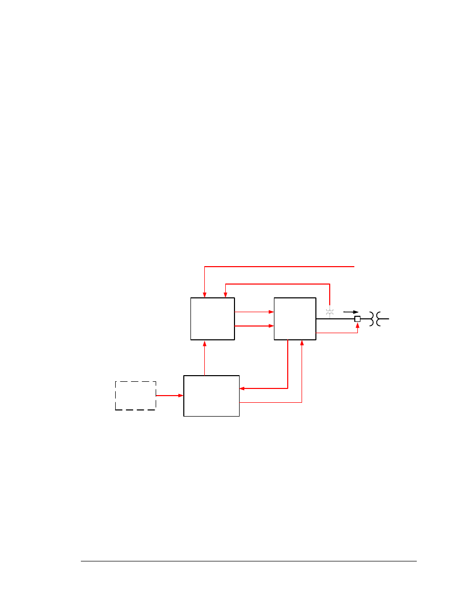
The dynamic models presented here are specific to the GE WTGs. The implementation
is structured in a fashion that is similar to other conventional generators. To construct a
complete WTG model, three device models are used:
•
Generator/converter model (interfaces with network and models several
hardware-related constraints.)
•
Electrical control model (includes closed and open loop reactive power
controls and provides for other system level features, e.g. governor
function, for future applications)
•
Turbine and turbine control model (mechanical controls, including blade
pitch control and power order to converter; over/under speed trips; rotor
inertia equation; wind power as a function of wind speed, blade pitch, and
rotor speed.)
A fourth, user-written model can be used to simulate a wind gust by varying input wind
speed to the turbine model. The user can also input wind speed vs. time sequences,
derived from field measurements or other sources.
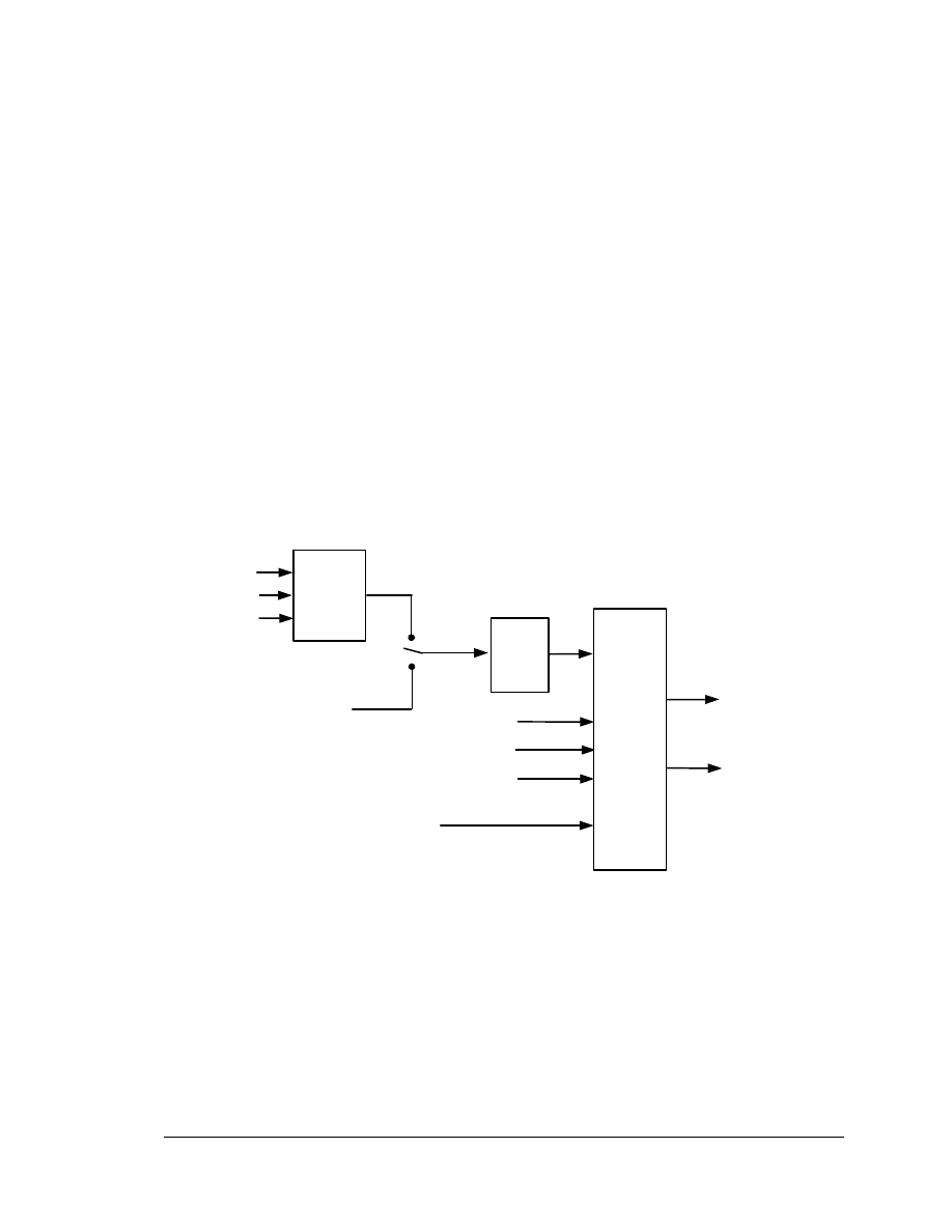
The overall connectivity of the models is shown in Figure 2-2.
Generator/
Converter
Model
P
gen
, Q
gen
Electrical
Control
Model
P & Q
Commands
Over/under
Voltage
Trip Signal
Turbine &
Turbine Control
Model
Wind
Speed
Wind Gust
Model
(User-written)
Power
Order
Over/under Speed
Trip Signal
V
reg bus
V
term
P
elec
Trip Signal
Figure 2-2. GE WTG Dynamic Models and Data Connectivity

GE-Power Systems Energy Consulting
Copyright 2002 General Electric Company, U.S.A.
3.1
GE WTG Modeling-v3-0.doc, 10/27/03
3. Modeling for Loadflow
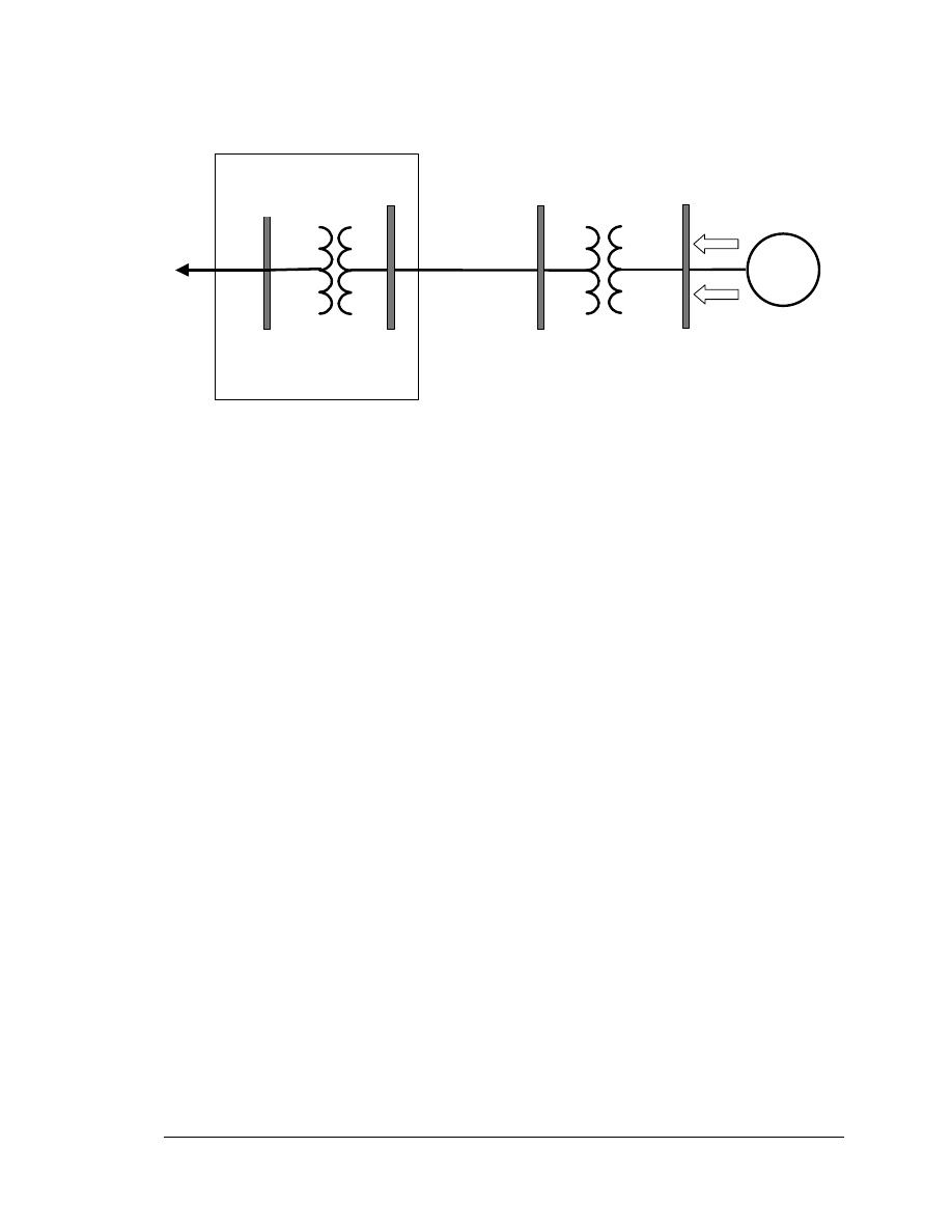
The modeling for load flow analysis is relatively simple, as shown in Figure 3-1. A
conventional generator is connected to a (PV) bus. For the 60Hz GE 1.5, each individual
WTG is connected to a 575V bus, and for the 60Hz GE 3.6, each individual WTG is
connected to a 4160V bus. The generator terminal bus is then connected to the collector
system bus through a suitably rated transformer. Typical collector system voltages are at
distribution levels (12.5 kV and 34.5 kV are common). For GE 3.6 applications, the
transformer will typically be 34.5kV/4160V, rated 4 MVA with a 6% leakage reactance.
Each GE 1.5 machine has a rated power output of 1.5 MW. The reactive power
capability of each individual machine is +0.95/-0.90 pf, which corresponds to Qmax =
0.49 MVAr and Qmin = -0.73 MVAr, and an MVA rating of 1.67 MVA. The minimum
steady-state power output for the WTG model is 0.2 MW.
Each GE 3.6 machine has a rated power output of 3.6 MW. The reactive power
capability of each individual machine is ±0.9 pf, which corresponds to Qmax = 1.74
MVAr and Qmin = -1.74 MVAr, and an MVA rating of 4.0 MVA. The minimum
steady-state power output for the WTG model is 0.5 MW.
Wind farms normally consist of a large number of individual WTGs. The wind farm
model may consist of a detailed representation of each WTG and the collector system.
Alternatively, a simpler model, which may be adequate for many bulk transmission
system studies, consists of a single WTG and transformer with MVA ratings equal to n
times the individual device ratings. Some equivalent impedance to reflect the aggregate
impact of the collector system can be included. A third alternative is to model groups of
WTGs by a single model, with a simplified representation of the collector system.
The supervisory control (WindVAR) is typically structured to measure the voltage at a
particular bus, often the point of interconnection (POI) with the transmission system, and
regulate this voltage by sending a reactive power command to all of the WTGs. Line
drop compensation may be used to regulate the voltage at a point some distance from the
voltage measurement bus. For loadflow modeling of the WindVAR, each WTG should
be set to regulate the same remote bus, located at the desired voltage regulation point.
GE-Power Systems Energy Consulting
Copyright 2002 General Electric Company, U.S.A.
3.2
GE WTG Modeling-v3-0.doc, 10/27/03
High Side Bus
(collector, e.g. 34.5kV)
Terminal Bus
P gen
Q gen
V
reg bus
V
term
Project Substation
Unit
Transformer
Point of
Interconnection
(POI) Bus
Substation
Transformer
Collector
Equivalent
Impedance
Figure 3-1 Loadflow Details
3.1
Initial conditions for dynamic simulation
The loadflow provides initial conditions for the dynamic simulations. The conditions
outlined above are generally applicable to the dynamic model presented below. The
maximum and minimum active and reactive power limits must be respected in order to
achieve a successful initialization. If the WTG electrical control or additional substation
controls are customized to meet a particular set of desired performance objectives, then
the loadflow must be initialized in accordance with those customized rules.

GE-Power Systems Energy Consulting
Copyright 2002 General Electric Company, U.S.A.
4.1
GE WTG Modeling-v3-0.doc, 10/27/03
4. Dynamic Model
This section presents the engineering assumptions, detailed structure, and data for each of
the component models.
4.1 Generator/Converter
Model
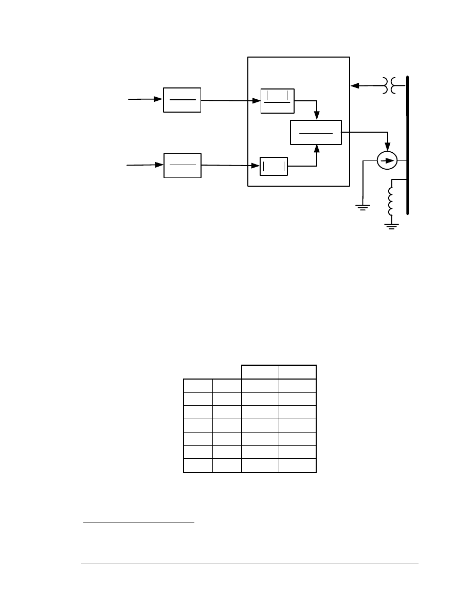
This model is the physical equivalent of the generator and provides the interface between
the WTG and the network. Unlike a conventional generator model it contains no
mechanical state variables for the machine rotor – these are included in the turbine
model. Further, unlike conventional generator models, all of the electrical/flux state
variables have been modified to reflect to the effective response to the higher level
commands from the electrical controls (i.e. the converter). The net result is an algebraic,
controlled-current source that computes the required injected current into the network in
response to the flux and active current commands from the excitation (converter) model.
For a given time step, the model holds the in-phase (active power) component of current
constant and holds constant q-axis voltage (d-axis flux) behind the subtransient reactance
(X”). The model includes two small time constants (20 msec) to represent converter
action. This is a reasonably accurate model of the combined behavior of the doubly-fed
generator and its rotor converter. The model is shown in Figure 4-1.
Several limits and trip functions related to the hardware capabilities are included in the
model. The generator will be tripped if the terminal voltage deviates from nominal (1
p.u.) by more than the voltage trip levels specified in Table 4-1, for more than the
corresponding trip times, also listed in Table 4-1. These levels may be different for some
projects. In addition, trip signals from the excitation (converter) model and turbine model
can also cause the generator to trip.
GE-Power Systems Energy Consulting
Copyright 2002 General Electric Company, U.S.A.
4.2
GE WTG Modeling-v3-0.doc, 10/27/03
V
term
From excitation
control model
E
q
"
I
Pcmd
I
P
Q
X"
P
*
+
+
im
re
jV
V
jQ
P
I
sorc
Iterate with network
solution
term
V
term
V
jX"
E
q
"
cmd
1
1+ 0.02s
1
1+ 0.02s
s0
s1
From excitation
control model
Figure 4-1 Generator/Converter Model (X”= 0.20 pu)
Table 4-1 WTG Generator/Converter Trip Levels and Times
[pu] [sec]
∆
V
trip
T
trip
-0.15 10.0
∆
V
trip
T
trip
-0.25 1.0
∆
V
trip
T
trip
-0.30 0.10
1
∆
V
trip
T
trip
-0.70 0.02
2
∆
V
trip
T
trip
+0.10 1.0
∆
V
trip
T
trip
+0.15 0.10
∆
V
trip
T
trip
+0.30 0.02
2
1
Machines equipped with low voltage ride through (LVRT); else 0.02 sec
2
Nominally instantaneous trip; 20 ms delay is recommended to improve simulation numerical behavior
GE-Power Systems Energy Consulting
Copyright 2002 General Electric Company, U.S.A.
4.3
GE WTG Modeling-v3-0.doc, 10/27/03
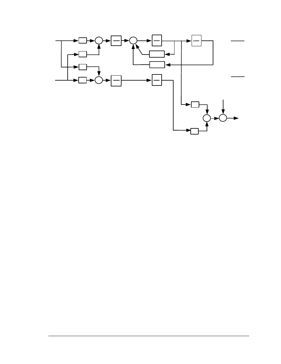
4.2
Excitation (Converter) Control Model
The Excitation Control Model dictates the active and reactive power to be delivered to
the system based on inputs from the turbine model (P
ord
) and from the supervisory VAR
controller (Q
ord
). Q
ord
can either come from a separate model or from the DVAR
Emulation function included in the Excitation Control Model. The design philosophy has
been to greatly simplify the model relative to the actual implementation used within the
equipment, while maintaining those aspects that are crucial to capturing the system
dynamic performance of interest. The model consists of the following control functions:
WindVAR Emulation
Open Loop Control Logic
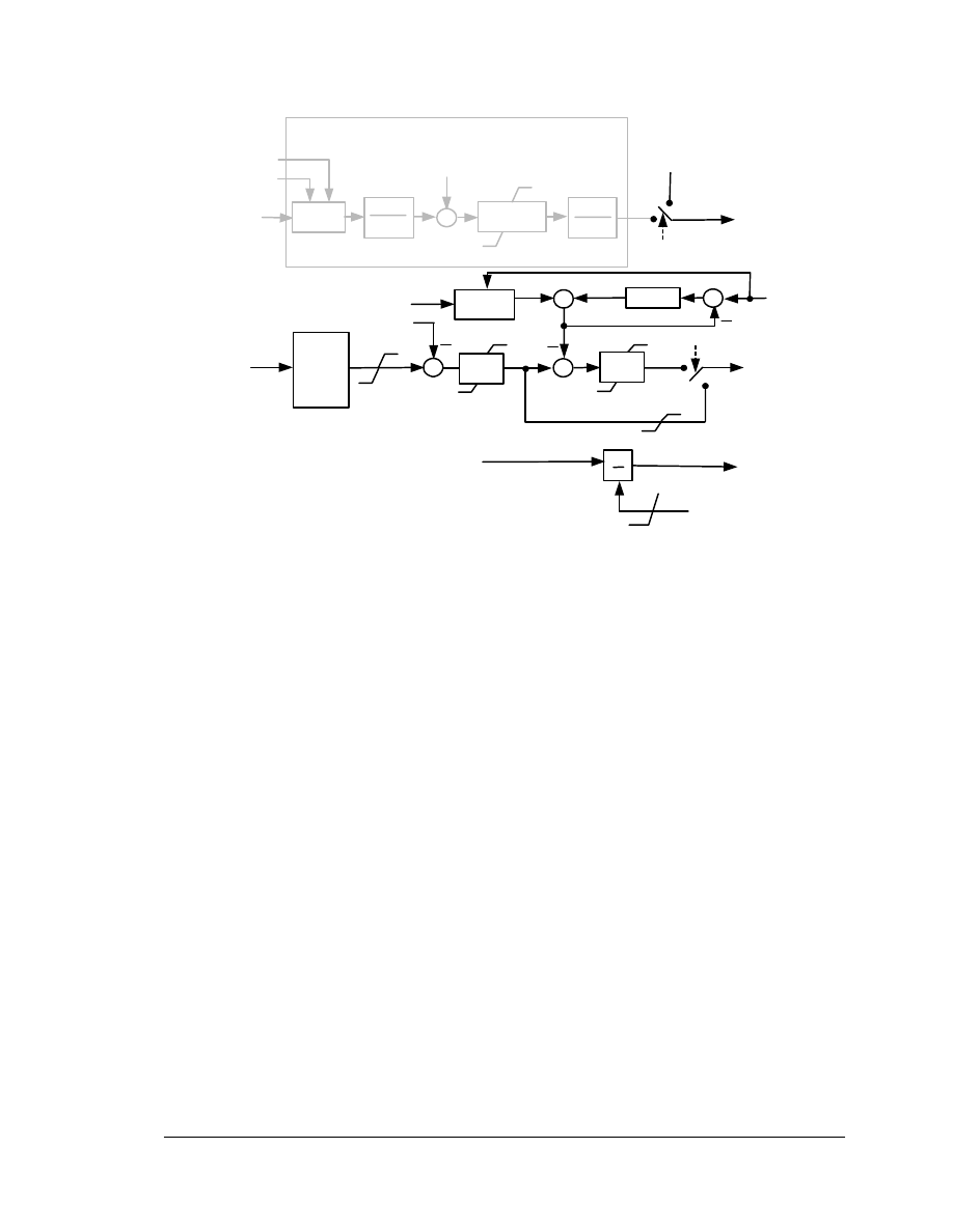
Electrical Controller
The overall block diagram for the Electrical Control model is shown in Figure 4-2; Figure
4-3 shows a more detailed representation.
From
supervisory
VAR
controller
E
q
"
cmd
Q
ord
I
Pcmd
Open
Loop
Control
Logic
WindVAR
Emulation
P
gen
Q
gen
V
reg
Q
cmd
P
gen
Q
gen
V
term
Electrical
Controller
Q
Q
P
ord
From
Wind Turbine
Model
To Generator
Model
Figure 4-2 Overall Excitation (Converter) Control Model
GE-Power Systems Energy Consulting
Copyright 2002 General Electric Company, U.S.A.
4.4
GE WTG Modeling-v3-0.doc, 10/27/03
K
pv
+ K
iv
/s
+
V
ref
WindVAR Emulation
1
1+ sT
v
+
1
1+ sT
r
V
reg
Q
max
Q
min
V - I Z
c
(vref)
From
Wind Turbine
Model
+
P
ord
V
term
0
varflg
1
From
Supervisory
VAR
Controller
Q
cmd
Q
gen
K
Qi
/ s
V
ref
V
max
V
−
I Z
C
V
term
+
K
Vi
/ s
V
term
+ XI
Qmax
V
min
E
q
"
cmd
To Generator
Model
0.7
0
vltflg
1
Q
ord
I
Pcmd
To Generator
Model
Q
min
Q
max
Open
Loop
Control
Logic
Q
ord
s0
s5
s4
s3
s1
V
c
1
/ sT
VZ
+
+
I
term
P
gen
Q
gen
s2
V
term
+ XI
Qmin
V
term
+ XI
Qmax
V
term
+ XI
Qmin
-
V
err
.
.
Figure 4-3 Electrical Control Model
WindVAR Emulation
The WindVAR Emulation function represents a simplified equivalent of the supervisory
VAR controller for the entire wind farm. The function monitors a specified bus voltage,
with optional line drop compensation, and compares it against the reference voltage. The
regulator itself is a PI controller plus a time constant, T
v
. The time constant reflects the
delays associated with cycle time, communication delay to the individual WTGs, and
additional high frequency attenuation needed to maintain stability. The measurement lag
is represented by the time constant T
r
. Table 4-3 includes suggested settings for the
WindVAR Emulation model. All settings are given in terms of rated MVA.
Open Loop Control Logic
The Open Loop Control Logic is responsive to large variations in system voltage, and is
inactive whenever the terminal voltage is within its normal range. The Open Loop
Control Logic is described by Table 4-2. The functions in this table represent the type of
optional open loop controls than were implemented to improve system performance for
large voltage deviations resulting from systems events. This feature was used in some
wind farms with GE WTGs before the implementation of present local closed loop
electrical controller described below. The Open Loop Control Logic forces the reactive
power to pre-specified levels as voltage deviations persist. As with all open loop

GE-Power Systems Energy Consulting
Copyright 2002 General Electric Company, U.S.A.
4.5
GE WTG Modeling-v3-0.doc, 10/27/03
controllers of this type, hysteresis is needed to avoid hunting. Once the voltage
thresholds are crossed and the open loop reactive power command is issued, the threshold
voltage is shifted up (or down for high voltage events) by a specified amount, V
hyst
. For
future projects with GE WTGS, this feature is not expected to be required. However,
representative values from earlier projects for the open loop control parameters are given
in Table 4-3.
Table 4-2 Open Loop Reactive Power Control Logic
Voltage Condition
For time duration
Open Loop Reactive Power
Command
V
term
< V
L1
t < T
L1
Q
L1
T
L1
< t < T
L2
Q
L2
t > T
L2
Q
L3
V
term
> V
H1
t < T
H1
Q
H1
T
H1
< t < T
H2
Q
H2
t > T
H2
Q
H3
Electrical Controller
The electrical controller model is a simplified representation of the converter/excitation
system. This controller monitors the generator reactive power, Q
gen
, and terminal
voltage, V
term
(or a remotely compensated voltage), to compute the voltage and current
commands E
q
”
cmd
and I
Pcmd
.
The model allows for the control of V
term
or Q
gen
. If the flag vltflg is set to 1, the terminal
voltage is compared against the reference voltage V
ref
, to create the voltage error V
err
.
This error is then multiplied by a gain and integrated to compute the voltage command
E
q
”
cmd
. The magnitude of the gain determines the effective time constant associated with
the voltage control loop. If the flag vltflg is set to 0, the integral of the error between Q
cmd
and Q
gen
is used directly to compute the voltage command E
q
”
cmd
to regulate Q
gen
. In both
cases E
q
”
cmd
is limited according to a time-varying limit that reflects hardware
characteristics and prevents unrealistic high or low values.
The current command I
Pcmd
is computed by dividing the power order, P
ord
, from the wind
turbine model over the generator terminal voltage V
term
.
Table 4-3 includes recommended settings for the Electrical Control model. All settings
are given in terms of rated MVA.

GE-Power Systems Energy Consulting
Copyright 2002 General Electric Company, U.S.A.
4.6
GE WTG Modeling-v3-0.doc, 10/27/03
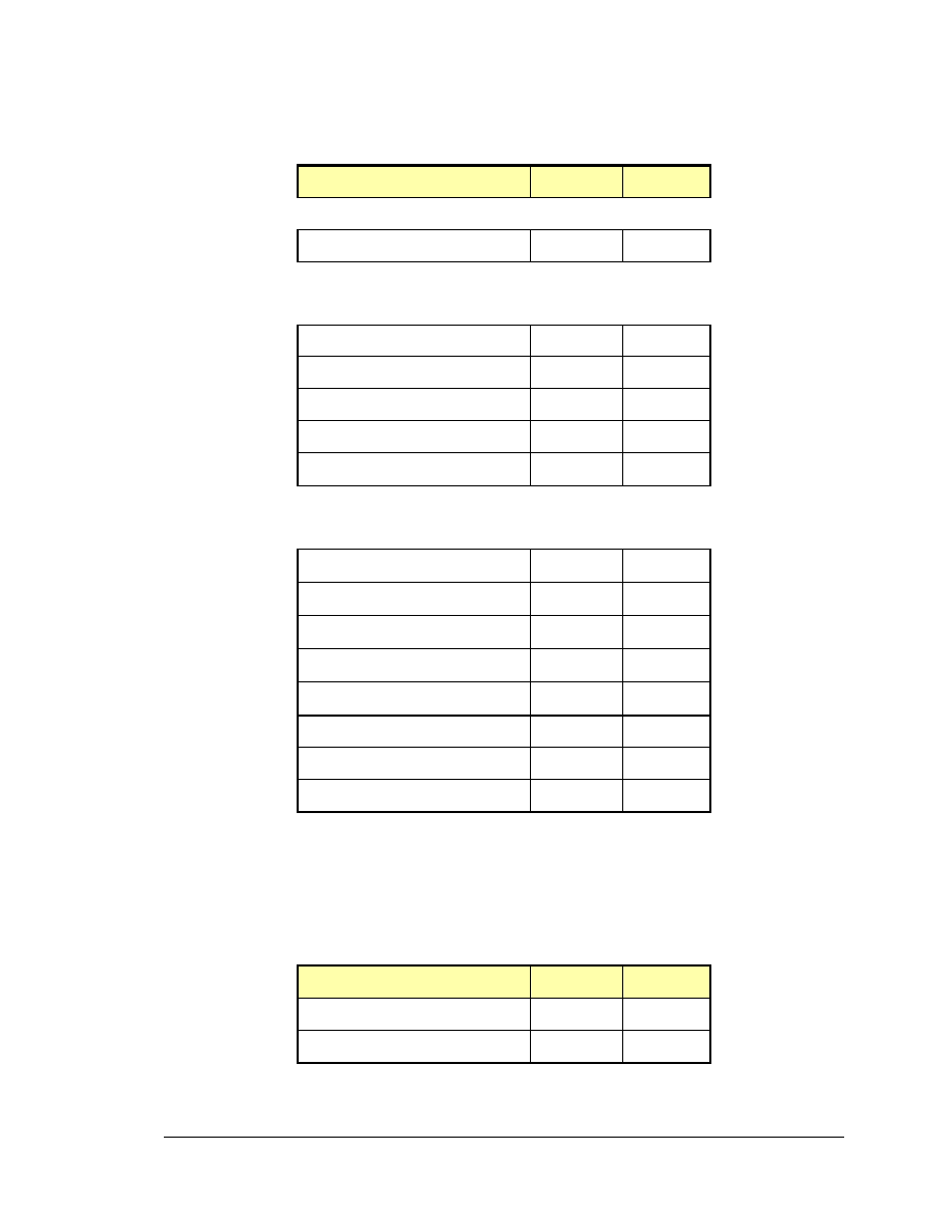
Table 4-3 WTG Electrical Control Parameters
(all power quantities are per unit on MVA base – 1.67MVA or 4.0 MVA)
Parameter Name
Recommended Value
T
r
0.05
T
v
0.05
K
pv
20
K
iv
2.0
K
Qi
0.05
K
Vi
20.0
T
vz
1.0
Q
max
0.29 (1.5) /0.432 (3.6)
Q
min
-0.432
XI
Qmax
0.07
XI
Qmin
-0.07
V
max
1.05
V
min
0.95
V
L1
0.9
V
H1
1.1
T
L1
0.1
T
L2
0.5
T
H1
0.1
T
H2
1.0
Q
L1
Q
cl
*
Q
L2
Q
cl
* (0.45 for older
projects)
Q
L3
Q
cl
*
Q
H1
Q
cl
*
Q
H2
-0.245
Q
H3
Q
cl
*
V
hyst
0.05
Z
c
0.0
* Qcl – closed-loop Q command is passed without modification. (can be indicated by
setting parameter to 0.)
GE-Power Systems Energy Consulting
Copyright 2002 General Electric Company, U.S.A.
4.7
GE WTG Modeling-v3-0.doc, 10/27/03
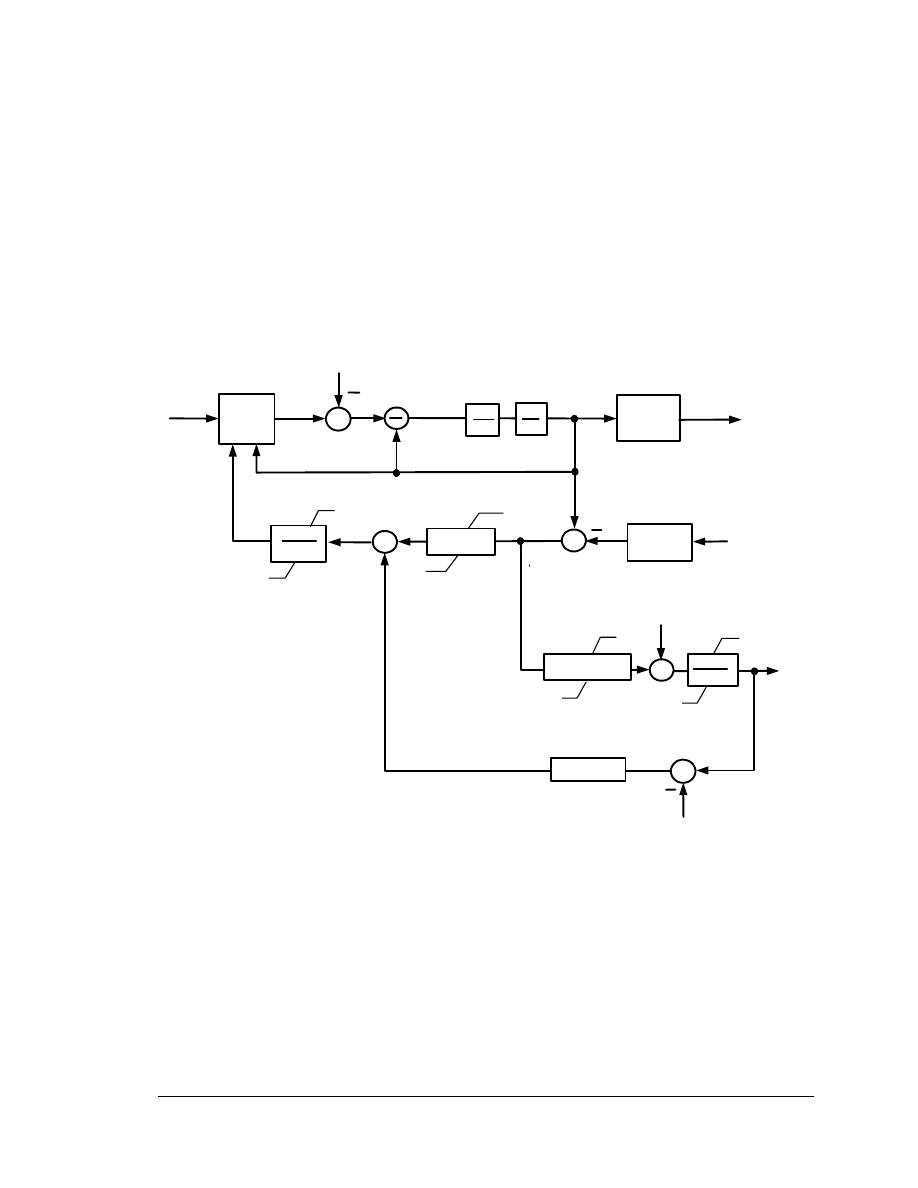
4.3
Wind Turbine & Turbine Control Model
The wind turbine model provides a simplified representation of a very complex electro-
mechanical system. The block diagram for the model is shown in Figure 4-4. In simple
terms, the function of the wind turbine is to extract as much power from the available
wind as possible without exceeding the rating of the equipment. The wind turbine model
represents all of the relevant controls and mechanical dynamics of the wind turbine. The
block labeled “Wind Power Model” is a moderately complex algebraic relationship
governing the mechanical shaft power that is dependent on wind velocity, rotor speed and
blade pitch. This model is described in Section 4.3.3.
Trip
Signal
1
1+ sT
p
P
mech
ω
Wind
Power
Model
Wind
Speed
Σ
θ
Blade
Pitch
Anti-windup on
Pitch Limits
K
ptrq
+ K
itrq
/ s
Torque Control
Pitch
Compensation
X
Anti-windup on
Power Limits
Over/Under
Speed
Trip
ω
Σ
Σ
1
s
1
2H
+
Speed
Setpoint
ω
ref
ω
err
Pitch Control
Kpp + Kip/s
P
elec
P
elec
ω
P
ord
1
1+ sT
pc
+
P
max
K
pc
+ K
ic
/ s
Σ
+
θ
min
&
d /dt
min
θ
θ
max
&
d /dt
max
θ
+
+
To
Electrical
Control
Model
To
Gen./Conv.
Model
From
Gen./Conv.
Model
ω
cmd
θ
P
min
&
d /dt
min
P
P
max
&
d /dt
max
P
:
T
acc
Figure 4-4. Wind Turbine Model Block Diagram
GE-Power Systems Energy Consulting
Copyright 2002 General Electric Company, U.S.A.
4.8
GE WTG Modeling-v3-0.doc, 10/27/03
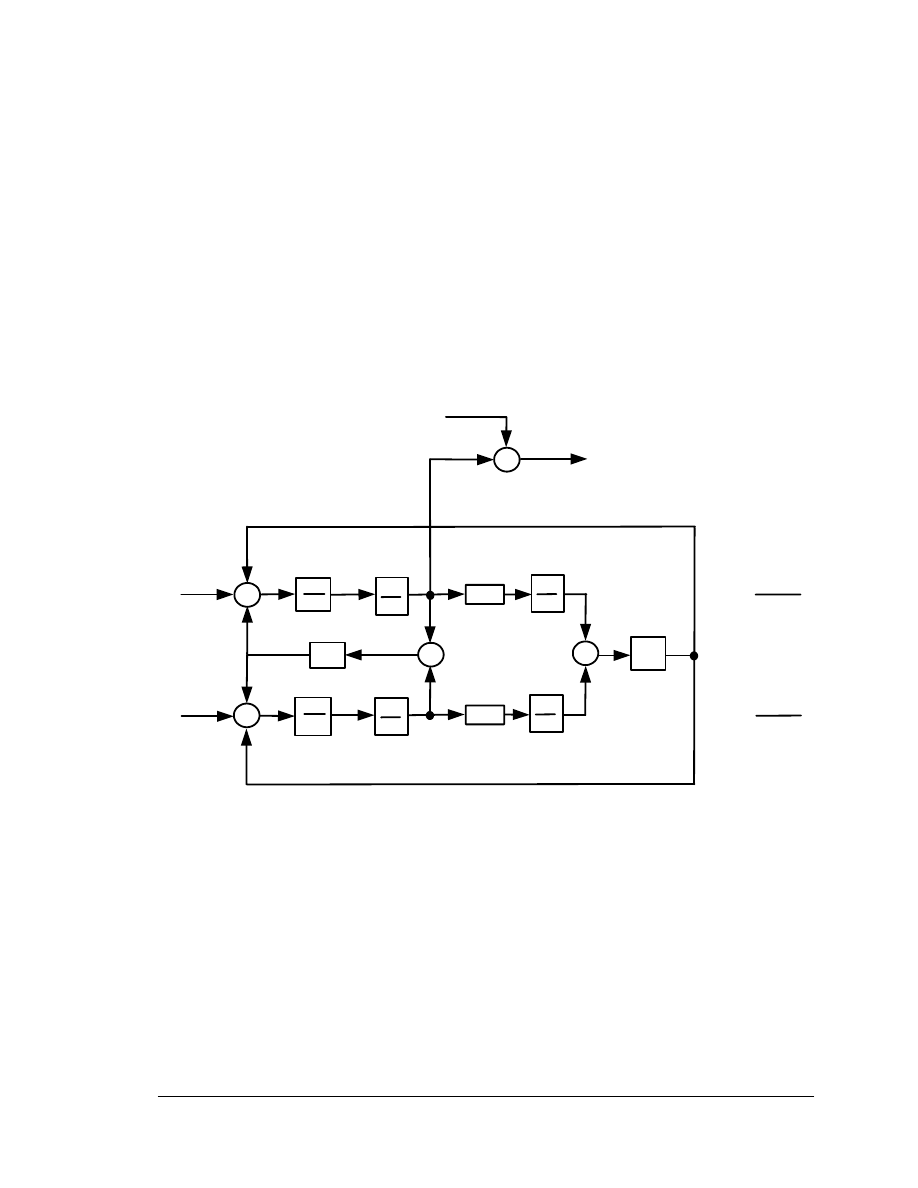
4.3.1 Rotor
Mechanical
Model
The upper part of Figure 4-2 includes the rotor inertia equation for the WTG rotor. This
equation uses the mechanical power from the Wind Power Model and the electrical
power from the Generator/Converter model to compute the rotor speed. This part of the
model can be extended to include a two-mass rotor model, with separate masses for the
turbine and generator. The relatively low natural torsional frequencies typical of wind
systems make this extension possible. Figures 4-5 and 4-6 show the two-mass rotor
model using physical and modal parameters, respectively.
T
mech
1
s
1
2H
ω
base
s6
1
s
Σ
K
tg
Σ
1
s
1
s
1
2H
g
Σ
D
tg
Σ
s7
s8
s9
+
+
+
+
+
T
elec
-
-
-
-
ω
ο
+
+
ω
Σ
-
ω
base
s8 +
ω
o
T
elec
=
P
elec
s6 +
ω
o
T
mech
=
P
mech
Figure 4-5. Two-Mass Rotor Model – Physical Parameters Model
GE-Power Systems Energy Consulting
Copyright 2002 General Electric Company, U.S.A.
4.9
GE WTG Modeling-v3-0.doc, 10/27/03
T
mech
s6
1
s
s7
+
T
elec
2ζ
n
ω
n
q
11
Σ
1
s
1
M
1
Σ
q
21
-
ω
n
2
-
-
+
s8
-
q
22
Σ
1
s
1
M
2
q
12
+
q
11
q
12
Σ
Σ
ω
ο
+
+
ω
+
+
s8 +
ω
o
T
elec
=
P
elec
s6 +
ω
o
T
mech
=
P
mech
Figure 4-6. Two-Mass Rotor Model – Modal Parameters Model
The data for the rotor mechanical model are given in Table 4-4.
GE-Power Systems Energy Consulting
Copyright 2002 General Electric Company, U.S.A.
4.10
GE WTG Modeling-v3-0.doc, 10/27/03
Table 4-4 WTG Rotor Mechanical Model Parameters
GE 1.5
GE 3.6
One-Mass Model
H (pu on turbine MW base)
4.64
5.19
Two-Mass Model -
Physical Parameters
H 4.32
4.29
H
g
0.62
0.90
K
tg
80.27
296.7
D
tg
1.5
1.5
ω
base
1.745 1.335
Two-Mass Model -
Modal Parameters
Μ
1
0.791 1.562
Μ
2
5.661 7.775
ζ
n
0.0610 1.575
ω
n
11.4 16.32
q
11
0.1411 0.2053
q
12
1.0
1.0
q
21
-0.990
-0.979
q
22
1.0
1.0
Overspeed and underspeed tripping logic is also included in the model. The related data
are listed in Table 4-5.
Table 4-5 Overspeed and Underspeed Tripping Thresholds
GE 1.5
GE 3.6
Overspeed trip
1.3 pu
1.3 pu
Underspeed trip
0.7 pu
0.7 pu

GE-Power Systems Energy Consulting
Copyright 2002 General Electric Company, U.S.A.
4.11
GE WTG Modeling-v3-0.doc, 10/27/03
4.3.2 Turbine
Control
Model
The lower part of Figure 4-2 is the model of the turbine control. The practical
implication of the turbine control is that when the available wind power is above the
equipment rating, the blades are pitched to reduce the mechanical power (P
mech
) delivered
to the shaft down to the equipment rating (1.0 pu). When the available wind power is
less than rated, the blades are set at minimum pitch to maximize the mechanical power.
In either case, the turbine control senses the shaft speed and tries to return the machine to
nominal speed. The dynamics of the pitch control are moderately fast, and can have
significant impact on dynamic simulation results.
The turbine control model sends a power order to the electrical control, requesting that
the converter deliver this power to the grid. The electrical control, as described in
Section 4.2, may or may not be successful in implementing this power order. The electric
power actually delivered to the grid is returned to the turbine model, for use in the
calculation of rotor speed setpoint. As discussed above, the dynamics of the electrical
controller are extremely fast.
Dynamically, the combination of blade pitch control and electric power order results in
two distinct operating conditions. For power levels below rated, the turbine speed will be
controlled primarily by the electric power order to the specified speed reference. For
power levels above rated, the rotor speed will be controlled primarily by the pitch control,
with the speed being allowed to rise above the reference transiently.
In this model, the blade position actuators are rate limited and there is short time constant
associated with the translation of blade angle to mechanical output. The pitch control
does not differentiate between shaft acceleration due to increase in wind speed or due to
system faults. In either case, the response is appropriate and relatively slow compared to
the electrical control.
The reference speed is normally 1.2 pu but is reduced for power levels below 75%. This
behavior is included in the model by using the following equation for speed reference
when the power is below 0.75 pu:
51
.
0
42
.
1
67
.
0
2
+
+
−
=
ω
P
P
ref
The speed reference slowly tracks changes in power with a time constant of
approximately 5 seconds.
The turbine control acts so as to smooth out electrical power fluctuations due to
variations in shaft power. By allowing the machine speed to vary around reference
speed, the inertia of the machine functions as a buffer to mechanical power variations.
The model does not include high and low wind speed cut-out for the turbine. In
situations where system performance questions hinge on this behavior, the user can
simply trip the machine.
Parameter values for the wind turbine control model are shown in Table 4-6. None of
these values should be modified by the user unless advised to by the manufacturer.

GE-Power Systems Energy Consulting
Copyright 2002 General Electric Company, U.S.A.
4.12
GE WTG Modeling-v3-0.doc, 10/27/03
Table 4-6 Turbine Control Parameters
(all quantities are per unit. on MW base)
Parameter Name
Recommended Value
K
pp
150.
K
ip
25.
T
p
(second)
0.01
Θ
max
(degrees)
27.
Θ
min
(degrees)
0.0
dθ/dt
max
(degrees/second)
10.0
dθ/dt
min
(degrees/second)
-10.0
P
max
(pu)
1.0
P
min
(pu)
0.1
dP/dt
max
pu/second)
0.45
dP/dt
min
(pu/second)
-0.45
K
pc
3.0
K
ic
30.0
K
ptrq
3.0
K
itrq
0.6
T
pc
0.05

GE-Power Systems Energy Consulting
Copyright 2002 General Electric Company, U.S.A.
4.13
GE WTG Modeling-v3-0.doc, 10/27/03
4.3.3 Wind Power Model
For power system simulations involving grid disturbances, it is a reasonable
approximation to assume that wind speed remains uniform for the 5 to 30 seconds typical
of such cases. However, the mechanical power delivered to the shaft is complex function
of wind speed, blade pitch angle and shaft speed. Further, with wind generation, the
impact of wind power fluctuations on the output of the machines is of interest. The
turbine model depends on the wind power model to provide this mapping.
The function of the wind power module is to compute the wind turbine mechanical power
(shaft power) from the energy contained in the wind, using the following formula:
P is the mechanical power extracted from the wind,
ρ
is the air density in kg/m
3
, A
r
is the
area swept by the rotor blades in m
2
, v
w
is the wind speed in m/sec, and C
p
is the is the
power coefficient, which is a function of
λ
and
θ
.
λ
is the ratio of the rotor blade tip
speed and the wind speed (v
tip
/v
w
),
θ
is the blade pitch angle in degrees. For the rigid
shaft representation used in this model, the relationship between blade tip speed and
generator rotor speed,
ω
, is a fixed constant, K
b
. The calculation of
λ
becomes:
λ
= K
b
(
ω
/v
w
)
For the GE WTGs, parameters given in Table 4.4 will result in P
mech
in pu on the unit’s
MW base.
Table 4-6. Wind Power Coefficients
GE 1.5
GE 3.6
½
ρ
A
r
0.00159 0.00145
K
b
56.6 69.5
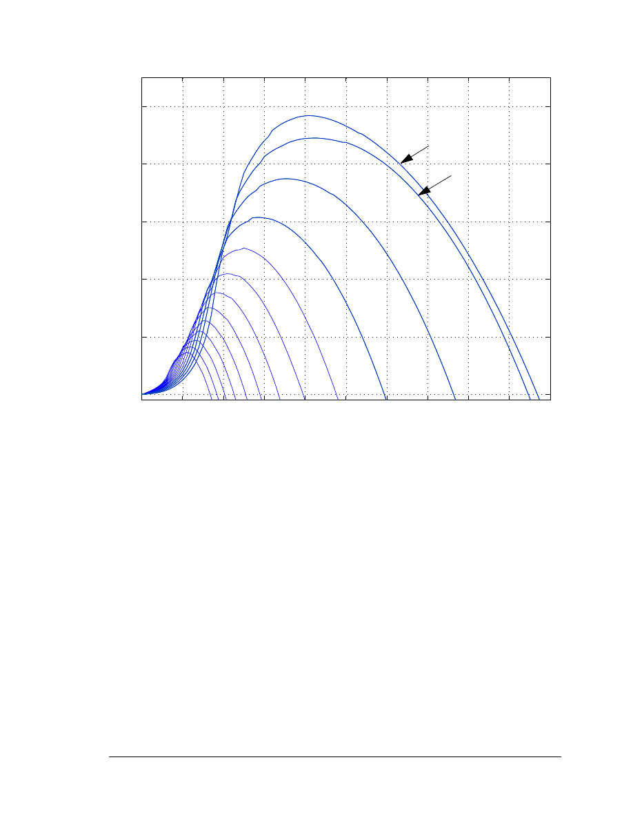
C
p
is a characteristic of the wind turbine and is usually provided as a set of curves
relating C
p
to
λ
, with
θ
as a parameter. The C
p
curves for the GE wind turbine are shown
in Figure 4-3. Curve fitting was performed to obtain the mathematical representation of
the C
p
curves used in the model:
j
j
i
j
i
i
p
C
λ
θ
α
=
λ
θ
∑
∑
=
=
4
0
,
4
0
)
,
(
The coefficients
α
i,j
are given in Table 4-7. The curve fit is a good approximation for
values of 2 <
λ
< 13. Values of
λ
outside this range represent very high and low wind
speeds, respectively, that are outside the continuous rating of the machine.
)
,
(
2
3
θ
λ
ρ
=
p
w
r
C
v
A
P
GE-Power Systems Energy Consulting
Copyright 2002 General Electric Company, U.S.A.
4.14
GE WTG Modeling-v3-0.doc, 10/27/03
0
2
4
6
8
10
12
14
16
18
20
0
0.1
0.2
0.3
0.4
0.5
λ
C
p
θ
=1
o
θ
=3
o
θ
=5
o
θ
=7
o
θ
=9
o
θ
=11
o
θ
=13
o
θ
=15
o
Figure 4-7. Wind Power C
p
Curves
Initialization of the wind power model recognizes two distinct states: 1) initial electrical
power (from the loadflow) is less than rated, or 2) initial electrical power equal to rated.
In either case, P
mech
= P
elec
is known from the loadflow and
ω = ω
ref
is set at the
corresponding value (1.2 pu if P > 0.75 pu). Then, using the C
p
curve fit equation, the
wind speed v
w
required to produce P
mech
with
θ
=
θ
min
is determined. (Notice from Figure
4-3, that two values of
λ
will generally satisfy the required C
p
for a given
θ.
The wind
speed v
w
, corresponding to the higher
λ
is used.) If P
mech
is less than rated, this value of
wind speed is used as the initial value. If P
mech
is equal to rated and the user-input value
of wind speed is greater than the
θ
=
θ
min
value, then
θ
is increased to produce rated P at
the specified value of wind speed.

GE-Power Systems Energy Consulting
Copyright 2002 General Electric Company, U.S.A.
4.15
GE WTG Modeling-v3-0.doc, 10/27/03
Table 4-7. Cp coefficients
α
i,j
i
j
a
ij
4 4
4.9686e-010
4 3
-7.1535e-008
4 2
1.6167e-006
4 1
-9.4839e-006
4 0
1.4787e-005
3 4
-8.9194e-008
3 3
5.9924e-006
3 2
-1.0479e-004
3 1
5.7051e-004
3 0
-8.6018e-004
2 4
2.7937e-006
2 3
-1.4855e-004
2 2
2.1495e-003
2 1
-1.0996e-002
2 0
1.5727e-002
1 4
-2.3895e-005
1 3
1.0683e-003
1 2
-1.3934e-002
1 1
6.0405e-002
1 0
-6.7606e-002
0 4
1.1524e-005
0 3
-1.3365e-004
0 2
-1.2406e-002
0 1
2.1808e-001
0 0
-4.1909e-001
4.4 Wind
Speed
Wind power fluctuations are relatively complex and stochastic in nature. The wind speed
variable is accessible to a user-written model that can be designed to apply various wind
fluctuations, including the following:
- Step of wind speed
- Wind gust following a (1 – cos A t) shape
- Wind speed variations derived from measurements
GE-Power Systems Energy Consulting
Copyright 2002 General Electric Company, U.S.A.
5.1
GE WTG Modeling-v3-0.doc, 10/27/03
5. Sample Simulation Results
This Section illustrates the performance of the GE PSLF model. The following three
simulations are included: i) comparison of the model response versus measured field
data; ii) simulation of a three-phase fault; and iii) simulation of an abrupt change in wind
speed.
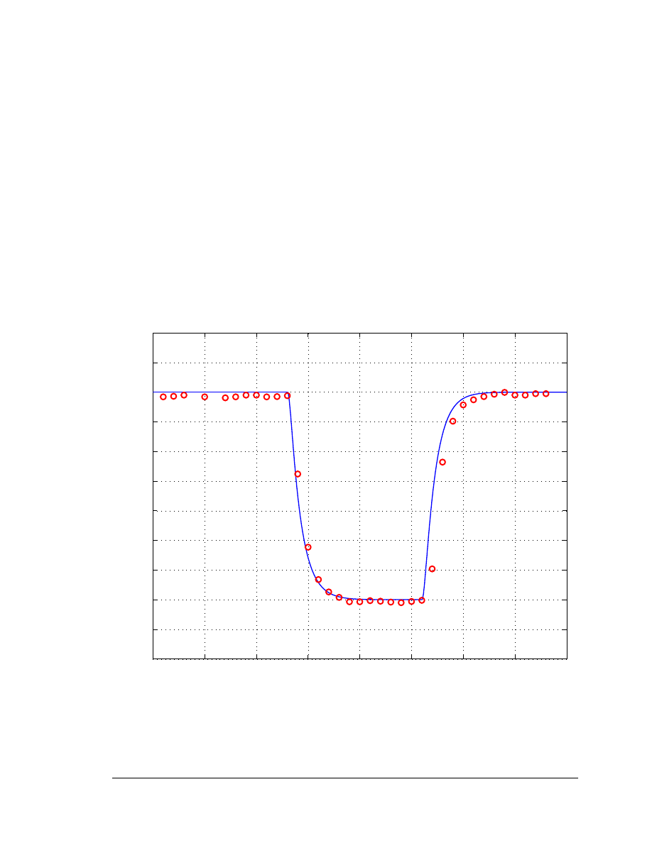
5.1
Comparison with Measured Data
Figure 5-1 compares the generator reactive power of the wind turbine model versus
measured data, for a up/down step in the reactive power order, Q
ord
. The discrete points
correspond to the measured data; the model response is the continuous trace. The model
response closely matches the field measurements.
0
5
10
15
20
25
30
35
40
−900
−800
−700
−600
−500
−400
−300
−200
−100
0
100
200
Time [sec]
Q
gen
[KVAr]
Figure 5-1. Generator Reactive Power – Response to a Step in Q Order
GE-Power Systems Energy Consulting
Copyright 2002 General Electric Company, U.S.A.
5.2
GE WTG Modeling-v3-0.doc, 10/27/03
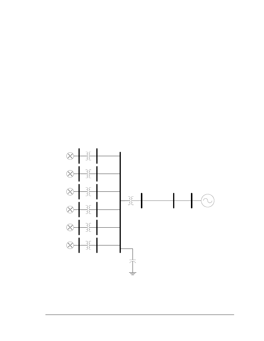
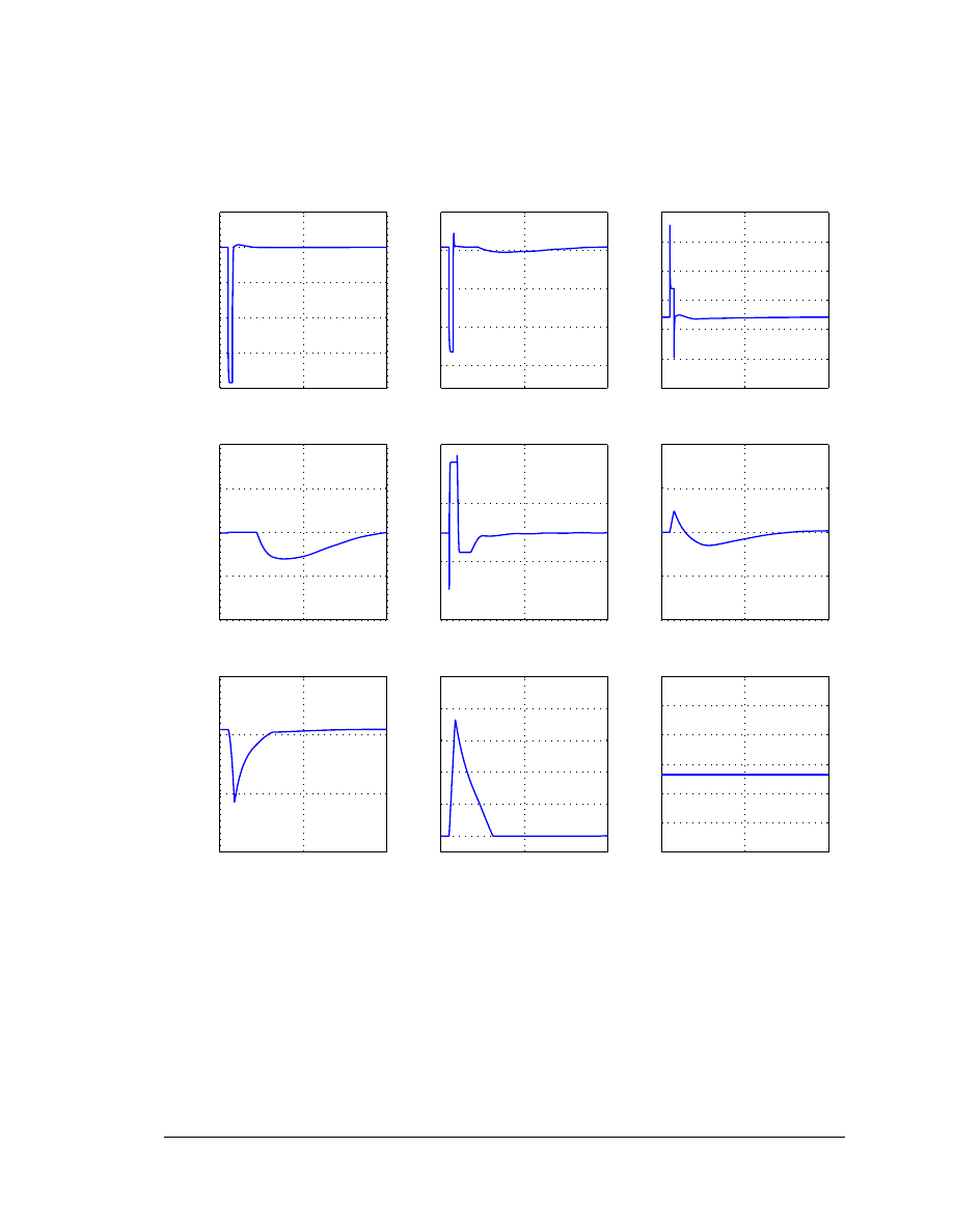
5.2
Response to Fault
The wind farm for this case consists of six wind turbines, WT1…WT6, connected to a
large power system with a single transmission line as shown in Figure 5.2. Each wind
turbine represents the aggregate of several 1.5 MW machines. The turbine-generator sets
are represented with a single mass model. A 30 cycle fault is applied at the point of
interconnection bus (POI). The low voltage trip point at 0.7 pu was reduced for this case
to demonstrate the control response. For this case, the wind speed, V
w
, is kept constant at
11.3 m/sec during the simulation.
Pertinent model variables are plotted in Figure 5-3. Following the fault, the speed (spd)
tends to increase. In response, the WT controller increases the pitch to reduce the
mechanical power provided by the wind turbine (Pmech). The generator terminal voltage
drops to 0.23 pu during the fault-on time and returns to 1.015 pu when the fault is
cleared. Its steady state value of 1 pu is reached at 4 sec. In response to a high voltage
following the removal of the fault, the reactive power order, Q
ord
, hits its Q
min
limit when
the fault is cleared.
WT
1
WT
2
WT
3
WT
4
WT
5
WT
6
POI
Figure 5-2. Power System Model
GE-Power Systems Energy Consulting
Copyright 2002 General Electric Company, U.S.A.
5.3
GE WTG Modeling-v3-0.doc, 10/27/03
0
10
20
0.2
0.4
0.6
0.8
1
1.2
V
te
rm
[pu]
Time [sec]
0
10
20
5
10
15
20
25
P
gen
[MW]
Time [sec]
0
10
20
−30
−20
−10
0
10
20
30
Q
gen
[MVAr]
Time [sec]
0
10
20
0.8
0.85
0.9
0.95
1
P
ord
[pu]
Time [sec]
0
10
20
−1
−0.5
0
0.5
Q
ord
[pu]
Time [sec]
0
10
20
1.1
1.15
1.2
1.25
1.3
spd [pu]
Time [sec]
0
10
20
10
15
20
25
P
mech
[MW]
Time [sec]
0
10
20
0
2
4
6
8
10
pitch [deg]
Time [sec]
0
10
20
10
10.5
11
11.5
12
12.5
13
V
w
[m/sec]
Time [sec]
Figure 5-3. Response to a 30 cycle system fault
GE-Power Systems Energy Consulting
Copyright 2002 General Electric Company, U.S.A.
5.4
GE WTG Modeling-v3-0.doc, 10/27/03
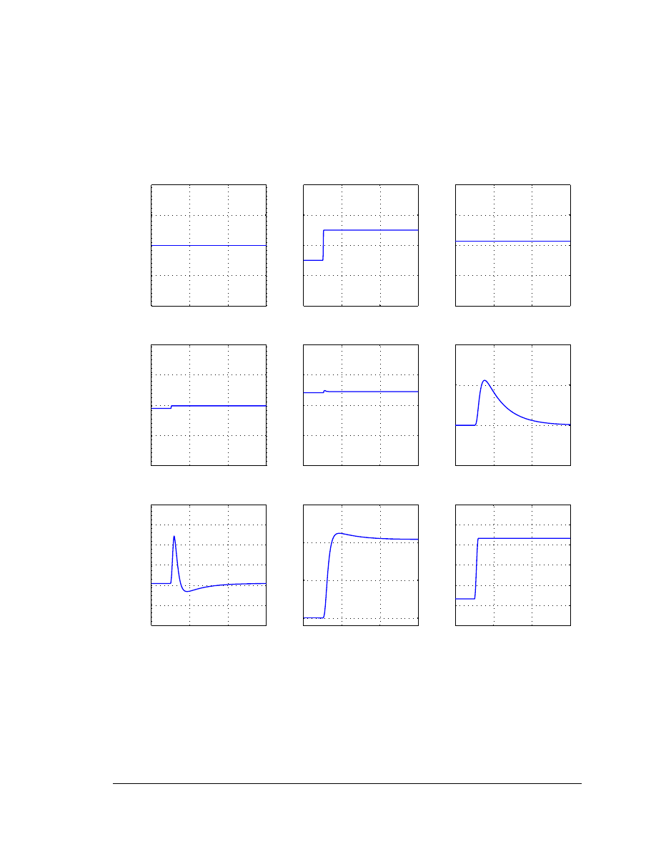
5.3
Response to Wind Step
Figure 5-4 shows the response of the system shown in Figure 5-1 to a change in wind
speed, V
w
, of 3 m/sec in a time span of 1 second. The WT controller adjusts the pitch to
10.4
o
to keep the speed, spd, at 1.2 pu.
0
10
20
30
0.98
0.99
1
1.01
1.02
V
te
rm
[pu]
Time [sec]
0
10
20
30
20.44
20.46
20.48
20.5
P
gen
[MW]
Time [sec]
0
10
20
30
−8
−7
−6
−5
−4
Q
gen
[MVAr]
Time [sec]
0
10
20
30
0.88
0.89
0.9
0.91
0.92
P
ord
[pu]
Time [sec]
0
10
20
30
−0.27
−0.265
−0.26
−0.255
−0.25
Q
ord
[pu]
Time [sec]
0
10
20
30
1.15
1.2
1.25
spd [pu]
Time [sec]
0
10
20
30
10
15
20
25
30
35
40
P
mech
[MW]
Time [sec]
0
10
20
30
0
5
10
15
pitch [deg]
Time [sec]
0
10
20
30
10
11
12
13
14
15
16
V
w
[m/sec]
Time [sec]
Figure 5-4. WTG Electrical Variables: Response to Wind Gust

GE-Power Systems Energy Consulting
Copyright 2002 General Electric Company, U.S.A.
6.1
GE WTG Modeling-v3-0.doc, 10/27/03
6. Other Technical Issues
6.1 Equivalencing
In practice, a wind farm has a local grid collecting the output from the machines into a
single point of connection to the grid. Since the wind farm is made up of many identical
machines, it is a reasonable approximation to parallel all the machines into a single
equivalent large machine behind a single equivalent reactance. This approach is
consistent with the model presented in this report. This approach is reasonable - up to a
point. Disturbances within the local collector grid cannot be analyzed, and there is some
potentially significant variation in the equivalent impedance for the connection to each
machine. A single machine equivalent requires the approximation that the power output
of all the machines will be the same at a given instant of time. For grid system impact
studies, simulations are typically performed with the initial wind of sufficient speed to
produce rated output on all machines. Under this condition, the assumption that all
machines are initially at the same (rated) output is not an approximation. Otherwise, this
assumption presumes that the geographic dispersion is small enough that the wind over
the farm is uniform. Simulations of bulk system dynamics using a single machine
equivalent is adequate for most planning studies.
Detailed modeling of the WTG collector system is possible. The inclusion of the
supervisory (WindVAR) control in each WTGs electrical control model provides an
emulation of the action of a single centralized control. An intermediate level of modeling
detail can also be used in which groups of WTGs, e.g. those on a single collector feeder,
are represented by a single equivalent model.
6.2
Applicability of Model to Other WTGs
This model was developed specifically for the GE 1.5 and 3.6 MW WTGs. The model is
applicable, with care, to other recent vintage GE WTGs and other WTGs, as long as the
basic principals of power conversion and control are the same. Just as with the
equivalencing, changing the MVA and MW bases for the device models will allow for
other machines to be represented.
In the broader sense, this model is not designed for, or intended to be used as, a general
purpose WTG. There are substantial variations between models and manufacturers.

GE-Power Systems Energy Consulting
Copyright 2002 General Electric Company, U.S.A.
7.1
GE WTG Modeling-v3-0.doc, 10/27/03
7. Conclusions
The wind turbine model presented in this report is based on presently available design
information, test data and extensive engineering judgment. The modeling of wind turbine
generators for bulk power system performance studies is still in a state of rapid evolution,
and is the focus of intense activity in many parts of the industry. More important, the GE
equipment is being continuously improved, to provide better dynamic performance.
These ongoing improvements necessitate continuing changes and improvements to these
models. This model is expected to give realistic and correct results when used for bulk
system performance studies. It is expected that as experience and additional hard test
data is obtained, these models will continue to evolve, in terms of parameter values and
structure.
Wyszukiwarka
Podobne podstrony:
[Engineering] Electrical Power and Energy Systems 1999 21 Dynamics Of Diesel And Wind Turbine Gene
DIN 61400 21 (2002) [Wind turbine generator systems] [Part 21 Measurement and assessment of power qu
[2006] Application of Magnetic Energy Recovery Switch (MERS) to Improve Output Power of Wind Turbine
[2006] Application of Magnetic Energy Recovery Switch (MERS) to Improve Output Power of Wind Turbine
CEI 61400 22 Wind turbine generator systems Required Design Documentation
20060028025 Wind Turbine Generator System
IEC 61400 11 Wind turbine generator systems en
20050253396 Variable Speed Wind Turbine Generator
CEI 61400 22 Wind turbine generator systems Required Design Documentation
Boost Converter Design For 20Kw Wind Turbine Generator
Wind Turbine Generator Rotor Construction (BackHome Magazine)(2s)
20060028025 Wind Turbine Generator System
IEC 61400 11 (2002) [Wind turbine generator systems Acoustic noise measurement techniques] [WIND][5
20050253396 Variable Speed Wind Turbine Generator
Dynamic Simulation Of Hybrid Wind Diesel Power Generation System With Superconducting Magnetic Energ
Modeling Of The Wind Turbine With A Doubly Fed Induction Generator For Grid Integration Studies
więcej podobnych podstron