Compute

Probabilistic Analysis Tutorial

8-1

Probabilistic Analysis

This tutorial will familiarize the user with the basic probabilistic analysis
capabilities of Slide. It will demonstrate how quickly and easily a
probabilistic slope stability analysis can be performed with Slide.

MODEL FEATURES:

• homogeneous, single material slope

• no water pressure (dry)

• circular slip surface search (Grid Search)

• random variables: cohesion, phi and unit weight

• type of probabilistic analysis: Global Minimum

The finished product of this tutorial (file: Tutorial 08 Probabilistic
Analysis.sli) can be found in the Examples > Tutorials folder in your
Slide installation folder.

Slide v.5.0 Tutorial

Manual

Probabilistic Analysis Tutorial

8-2

Model

This tutorial will be based on the same model used for Tutorial 1, so let’s

first read in the Tutorial 1 file.

Select: File

→ Open

Navigate to the Examples > Tutorials folder in your Slide installation
folder, and open the Tutorial 01 Quick Start.sli file.

Project Settings

To carry out a Probabilistic Analysis with Slide, the first thing that must

be done, is to select the Probabilistic Analysis option in the Project

Settings dialog.

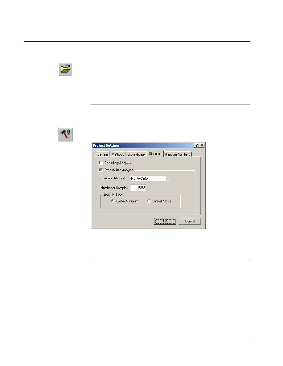
Select: Analysis

→ Project Settings

In the Project Settings dialog, select the Statistics tab, and select the
Probabilistic Analysis checkbox. Select OK.

Global Minimum Analysis

Note that we are using the default Probabilistic Analysis options:

• Sampling Method = Monte Carlo

• Number of Samples = 1000

• Analysis Type = Global Minimum

When the Analysis Type = Global Minimum, this means that the

Probabilistic Analysis is carried out on the Global Minimum slip surface

located by the regular (deterministic) slope stability analysis.

Slide v.5.0 Tutorial

Manual

Probabilistic Analysis Tutorial

8-3

The safety factor will be re-computed N times (where N = Number of

Samples) for the Global Minimum slip surface, using a different set of

randomly generated input variables for each analysis.

Notice that a Statistics menu is now available, which allows you to define

almost any model input parameter, as a random variable.

Defining Random Variables

In order to carry out a Probabilistic Analysis, at least one of your model

input parameters must be defined as a Random Variable. Random

variables are defined using the options in the Statistics menu.

For this tutorial, we will define the following material properties as

Random Variables:

• Cohesion

• Friction Angle

• Unit Weight

This is easily done with the Material Statistics dialog.

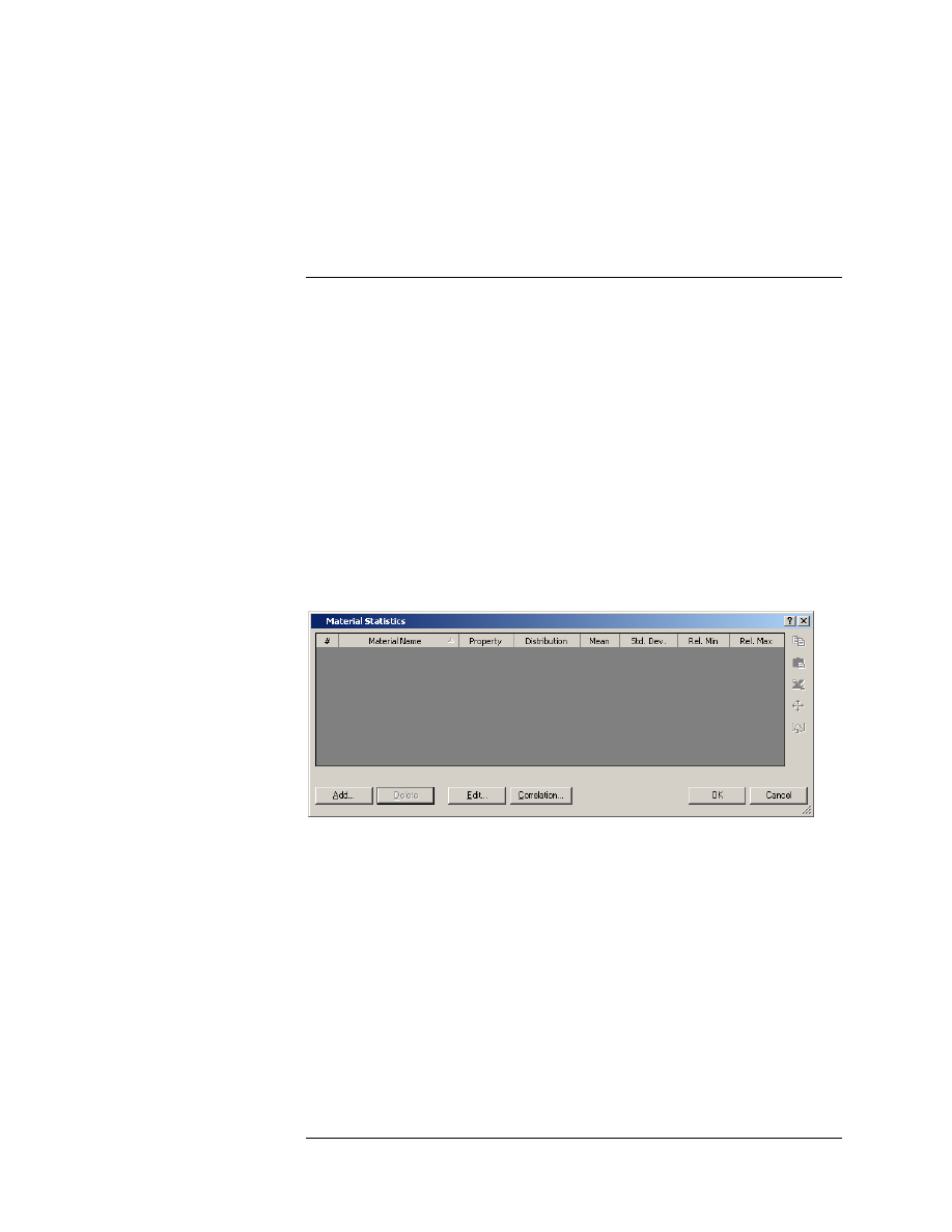
Select: Statistics

→ Materials

You will see the Material Statistics dialog.

First, you must select the Random Variables that you wish to use. This

can be done with either the Add or the Edit options, in the Material

Statistics dialog. Let’s use the Add option.

Select the Add button in the Material Statistics dialog.

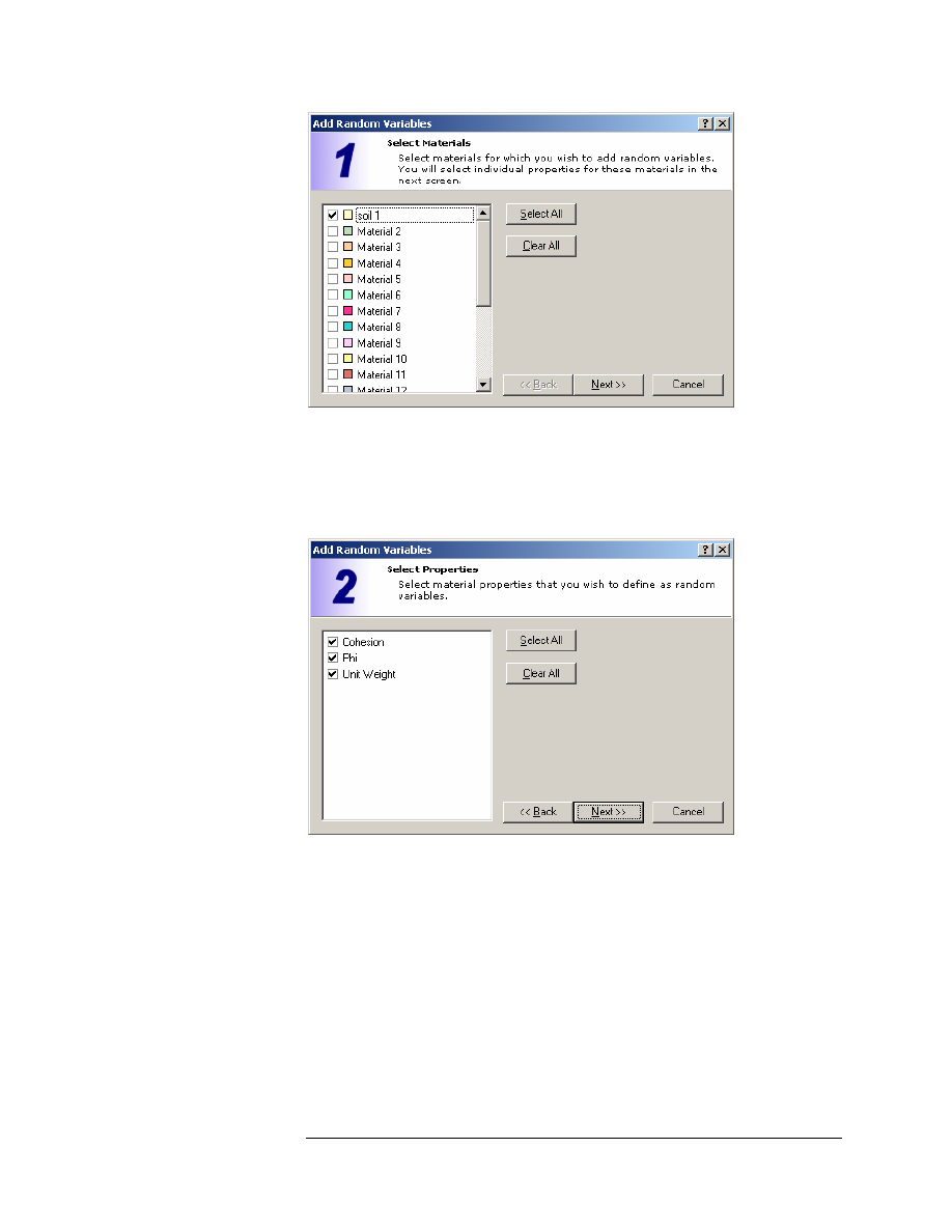
When using the Add option, you will see a series of three dialogs, in a

“wizard” format, which allow you to quickly select the material properties

that you wish to define as Random Variables.

The first dialog allows you to select the materials.

Slide v.5.0 Tutorial

Manual

Probabilistic Analysis Tutorial

8-4

Select the checkbox for the “soil 1” material (our slope model only uses this
one material type). Select the Next button.

The second dialog allows you to select the material properties that you

would like to define as Random Variables.

Select the checkboxes for Cohesion, Phi and Unit Weight. Select the Next
button.

The final dialog allows you to select a Statistical Distribution for the

Random Variables.

We will be using the default (Normal Distribution), so just select the
Finish button.

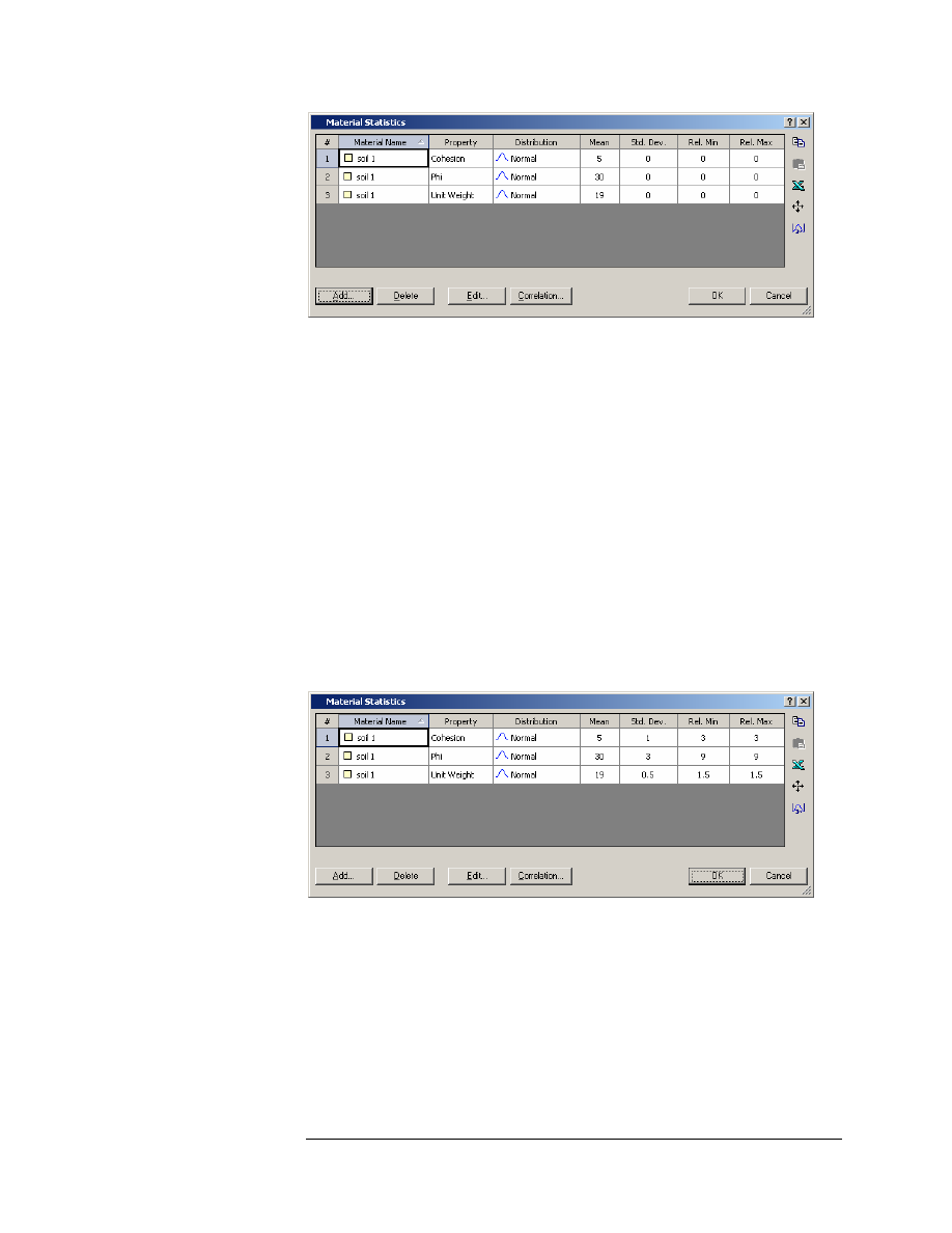
You will be returned to the Material Statistics dialog, which should now

appear as follows:

Slide v.5.0 Tutorial

Manual

Probabilistic Analysis Tutorial

8-5

In the Material Statistics dialog, the material properties which you

selected as Random Variables, now appear in the dialog in a spreadsheet

format. This allows you to easily define the statistical distribution for

each random variable.

In order to complete the process of defining the Random Variables, we

must enter:

• the Standard Deviation, and

• Minimum and Maximum values

for each variable, in order to define the statistical distribution of each

random variable.

Enter the values of Standard Deviation, Relative Minimum and Relative
Maximum for each variable, as shown below. When you are finished,
select OK.

NOTE:

• The Minimum and Maximum values are specified as RELATIVE

values (i.e. distances from the MEAN value), rather than as absolute

values, because this simplifies data input.

Slide v.5.0 Tutorial

Manual

Probabilistic Analysis Tutorial

8-6

• For a NORMAL distribution, 99.7 % of all samples should fall within

3 standard deviations of the mean value. Therefore it is

recommended that the Relative Minimum and Relative Maximum

values are equal to at least 3 times the standard deviation, to ensure

that a complete (non-truncated) NORMAL distribution is defined.

• For more information about Statistical Distributions, please see the

Probabilistic Analysis section of the Slide Help system.

That’s all we need to do. We have defined 3 Random Variables (cohesion,

friction angle and unit weight) with Normal distributions.

We can now run the Probabilistic Analysis.

Compute

First, let’s save the file with a new file name: prob1.sli.

Select: File

→ Save As

Use the Save As dialog to save the file. Now select Compute.

Select: Analysis

→ Compute

NOTE:

• When you run a Probabilistic Analysis with Slide, the regular

(deterministic) analysis is always computed first.

• The Probabilistic Analysis automatically follows. The progress of the

analysis is indicated in the Compute dialog.

Slide v.5.0 Tutorial

Manual

Probabilistic Analysis Tutorial

8-7

Interpret

To view the results of the analysis:

Select: Analysis

→ Interpret

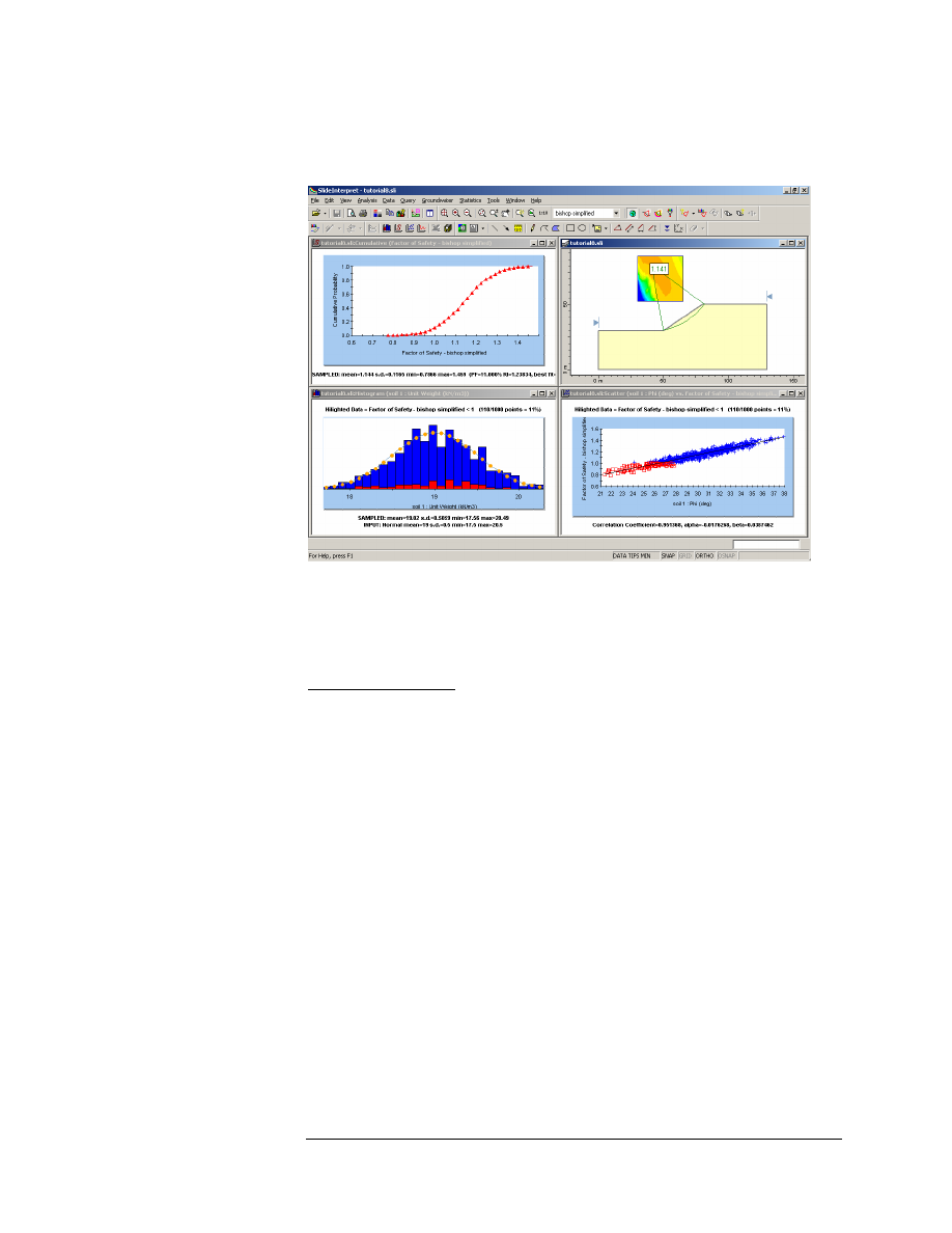
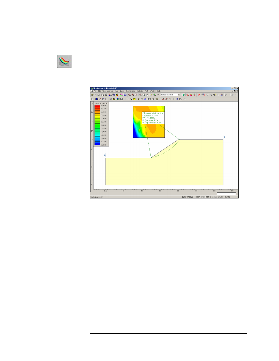
This will start the Slide INTERPRET program. You should see the

following figure.

Figure 8-1: Results after probabilistic analysis.

The primary results of the probabilistic analysis, are displayed beside the

slip center of the deterministic global minimum slip surface. Remember

that when the Probabilistic Analysis Type = Global Minimum, the

Probabilistic Analysis is only carried out on this surface.

This includes the following:

• FS (mean) – the mean safety factor

• PF – the probability of failure

• RI – the Reliability Index

Slide v.5.0 Tutorial

Manual

Probabilistic Analysis Tutorial

8-8

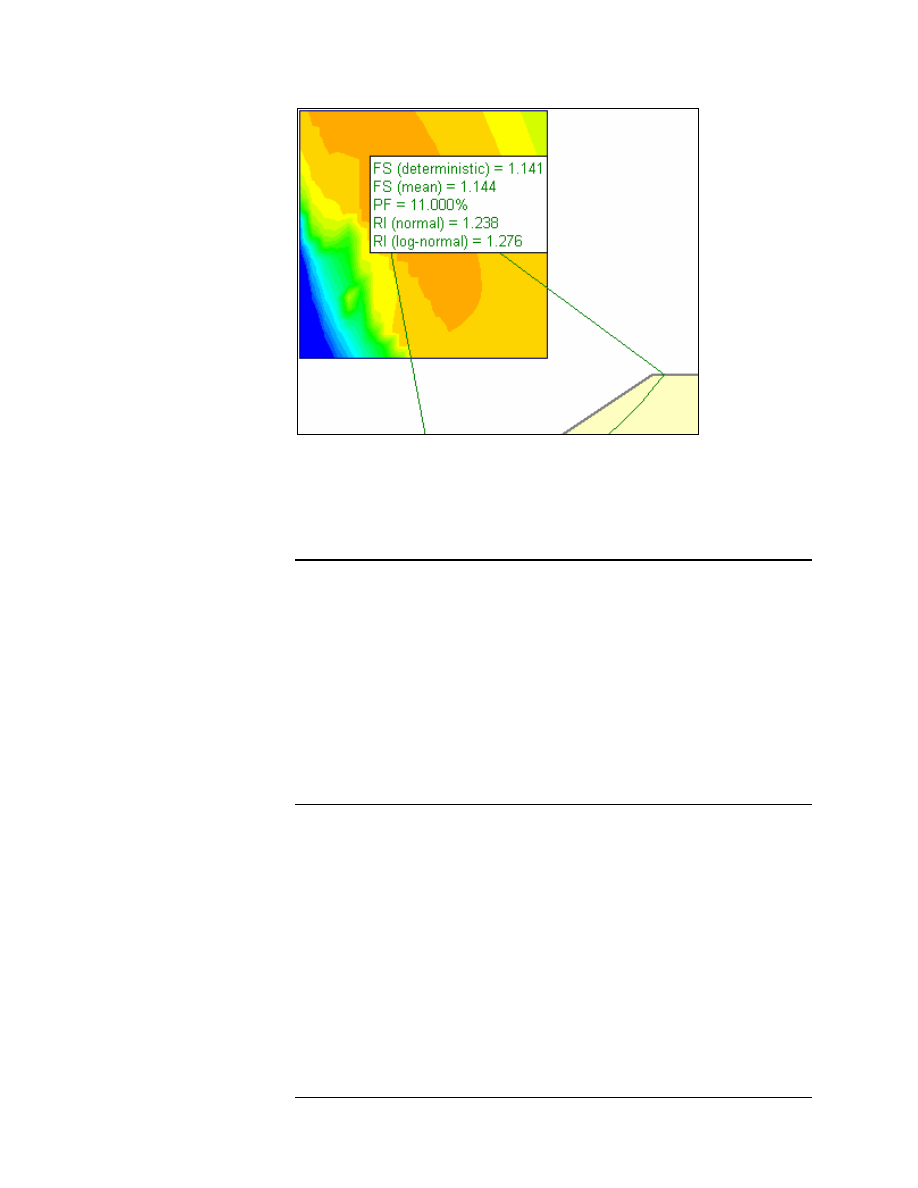
Figure 8-2: Summary of results after probabilistic analysis.

These results are discussed below.

Deterministic Safety Factor

The Deterministic Safety Factor, FS (deterministic), is the safety factor

calculated for the Global Minimum slip surface, from the regular (non-

probabilistic) slope stability analysis.

This is the same safety factor that you would see if you were only

running a regular (deterministic) analysis, and were NOT running a

Probabilistic Analysis.

The Deterministic Safety Factor is the value of safety factor when all

input parameters are exactly equal to their mean values.

Mean Safety Factor

The Mean Safety Factor is the mean (average) safety factor, obtained

from the Probabilistic Analysis. It is simply the average safety factor, of

all of the safety factors calculated for the Global Minimum slip surface.

In general, the Mean Safety Factor should be close to the value of the

deterministic safety factor, FS (deterministic). For a sufficiently large

number of samples, the two values should be nearly equal.

Slide v.5.0 Tutorial

Manual

Probabilistic Analysis Tutorial

8-9

Probability of Failure

The Probability of Failure is simply equal to the number of analyses with

safety factor less than 1, divided by the total Number of Samples.

100%

numfailed

numsamples

Eqn. 1

For this example, PF = 11%, which means that 110 out of 1000 samples,

produced a safety factor less than 1.

Reliability Index

The Reliability Index is another commonly used measure of slope

stability, after a probabilistic analysis.

The Reliability Index is an indication of the number of standard
deviations which separate the Mean Safety Factor from the critical safety

factor ( = 1).

The Reliability Index can be calculated assuming either a Normal or

Lognormal distribution of the safety factor results. The actual best fit

distribution is listed in the Info Viewer, and indicates which value of RI

is more appropriate for the data.

RI (Normal)

If it is assumed that the safety factors are Normally distributed, then

Equation 2 is used to calculate the Reliability Index.

−

Eqn.

where:

= reliability index

= mean safety factor

= standard deviation of safety factor

A Reliability Index of at least 3 is usually recommended, as a minimal

assurance of a safe slope design. For this example, RI = 1.238, which

indicates an unsatisfactory level of safety for the slope.

Slide v.5.0 Tutorial

Manual

Probabilistic Analysis Tutorial

8-10

RI (Lognormal)

If it is assumed that the safety factors are best fit by a Lognormal

distribution, then Equation 3 is used to calculate the Reliability Index.

ln(1

)













Eqn. 3

where

µ = the mean safety factor, and V = coefficient of variation of the

safety factor ( =

σ / µ ).

For more information about the Reliability Index, see the Slide Help

system.

Histogram Plots

Histogram plots allow you to view:

• The distribution of samples generated for the input data random

variable(s).

• The distribution of safety factors calculated by the probabilistic

analysis.

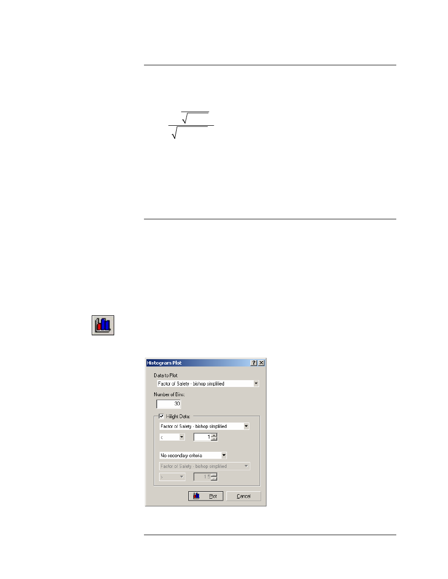
To generate a Histogram plot, select the Histogram Plot option from the

toolbar or the Statistics menu.

Select: Statistics

→ Histogram Plot

You will see the Histogram Plot dialog.

Slide v.5.0 Tutorial

Manual

Probabilistic Analysis Tutorial

8-11

Let’s first view a histogram of Safety Factor. Set the Data to Plot = Factor
of Safety – Bishop Simplified. Select the Highlight Data checkbox. As the
highlight criterion, select “Factor of Safety – Bishop Simplified < 1”. Select
the Plot button, and the Histogram will be generated.

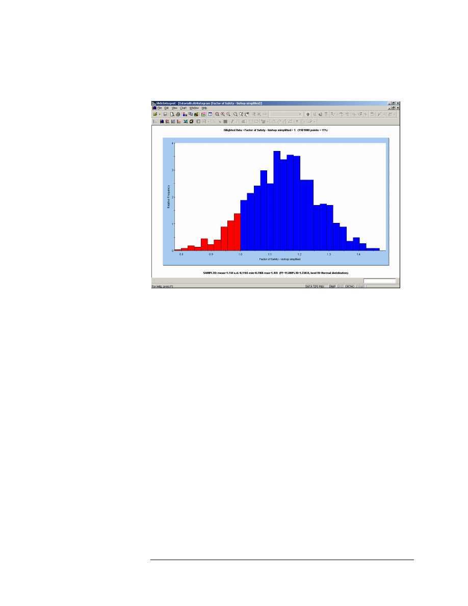
Figure 8-3: Histogram of Safety Factor.

As you can see on the histogram, the highlighted data (red bars) shows

the analyses which resulted in a safety factor less than 1.

• This graphically illustrates the Probability of Failure, which is equal

to the area of the histogram which is highlighted (FS < 1), divided by

the total area of the histogram.

• The statistics of the highlighted data are always listed at the top of

the plot. In this case, it is indicated that 110 / 1000 points, have a

safety factor less than 1. This equals 11%, which is the

PROBABILITY OF FAILURE (for the Bishop analysis method).

In general, the Highlight data option allows you to highlight any user-

defined subset of data on a histogram (or scatter plot), and obtain the

statistics of the highlighted (selected) data subset.

You can display the Best Fit distribution for the safety factor data, by

right-clicking on the plot, and selecting Best Fit Distribution from the

popup menu. The Best Fit Distribution will be displayed on the

Histogram. In this case, the best fit is a Normal Distribution, as listed at

the bottom of the plot.

Slide v.5.0 Tutorial

Manual

Probabilistic Analysis Tutorial

8-12

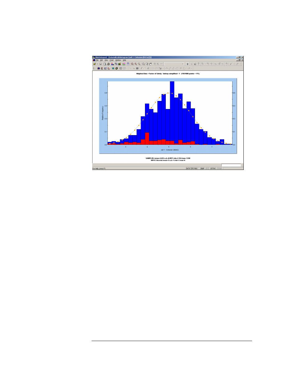
Let’s create a plot of the Cohesion random variable. Right-click on the
plot and select Change Plot Data. Set the Data to Plot = soil 1 : Cohesion.
Select Done.

Figure 8-4: Histogram Plot of Cohesion.

This plot shows the actual random samples which were generated by the

Monte Carlo sampling of the statistical distribution which you defined for

the Cohesion random variable. Notice that the data with Bishop Safety

Factor < 1 is still highlighted on the plot.

Note the following information at the bottom of the plot:

• The SAMPLED statistics, are the statistics of the raw data generated

by the Monte Carlo sampling of the input distribution.

• The INPUT statistics, are the parameters of the input distribution

which you defined for the random variable, in the Material Statistics

dialog.

In general, the SAMPLED statistics and the INPUT statistics will not be

exactly equal. However, as the Number of Samples increases, the

SAMPLED statistics should approach the values of the INPUT

parameters.

The distribution defined by the INPUT parameters is plotted on the

Histogram. The display of this curve can be turned on or off, by right-

clicking on the plot, and toggling the Input Distribution option.

Now right-click on the plot again, and select Change Plot Data. Change
the Data to Plot to soil 1 : Phi. Select Done.

Slide v.5.0 Tutorial

Manual

Probabilistic Analysis Tutorial

8-13

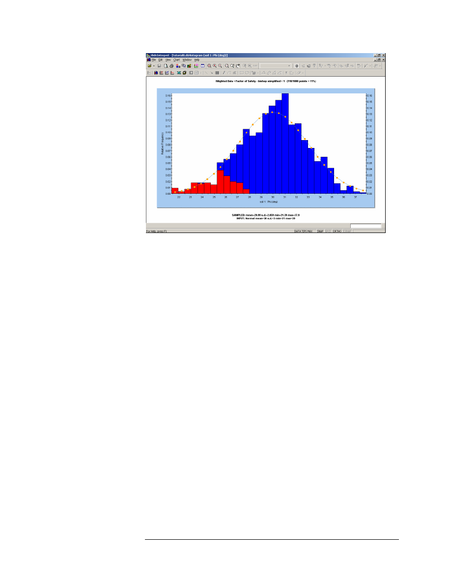
Figure 8-5: Histogram Plot of Friction Angle.

Notice the data with Bishop Safety Factor < 1, highlighted on the plot.

With respect to the Friction Angle random variable, it is clear that failure

corresponds to the lowest friction angles which were generated by the

random sampling.

Slide v.5.0 Tutorial

Manual

Probabilistic Analysis Tutorial

8-14

Cumulative Plots

To generate a Cumulative plot, select the Cumulative Plot option from

the toolbar or the Statistics menu.

Select: Statistics

→ Cumulative Plot

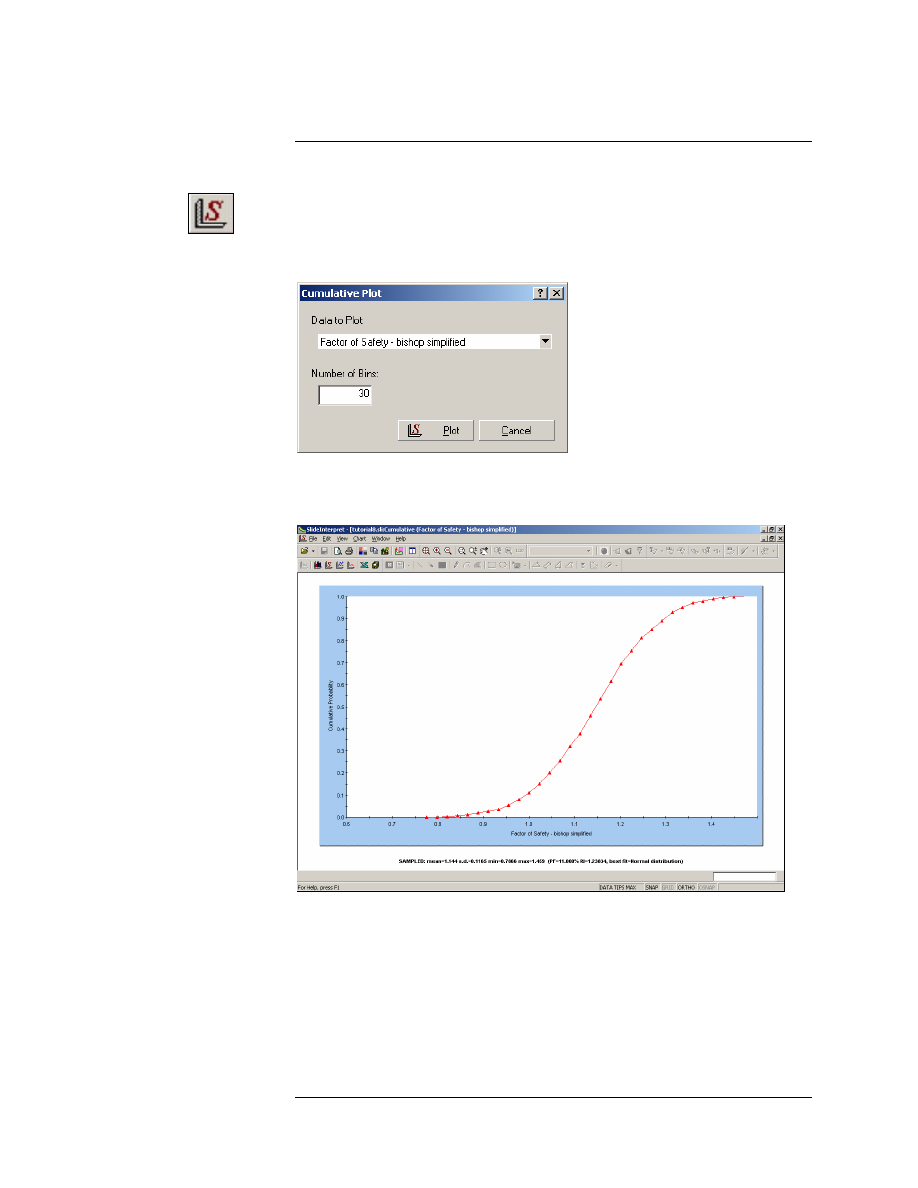
You will see the Cumulative Plot dialog.

Select the Data to Plot = Factor of Safety – Bishop Simplified. Select the
Plot button.

Figure 8-6: Cumulative Plot of Safety Factor.

A Cumulative distribution plot represents the cumulative probability

that the value of a random variable will be LESS THAN OR EQUAL TO

a given value.

Slide v.5.0 Tutorial

Manual

Probabilistic Analysis Tutorial

8-15

When we are viewing a Cumulative Plot of Safety Factor, the Cumulative

Probability at Safety Factor = 1, is equal to the PROBABILITY OF

FAILURE.

Let’s verify this as follows.

Sampler Option

The Sampler Option on a Cumulative Plot, allows you to easily determine

the coordinates at any point along the Cumulative distribution curve.

1. Right-click on the Cumulative Plot, and select the Sampler option.

2. You will see a dotted vertical line on the plot. This is the “Sampler”,

and allows you to graphically obtain the coordinates of any point on

the curve. You can do this as follows.

3. Click AND HOLD the LEFT mouse button on the plot. Now drag the

mouse along the plot. You will see that the Sampler follows the

mouse, and continuously displays the coordinates of points on the

Cumulative plot curve.

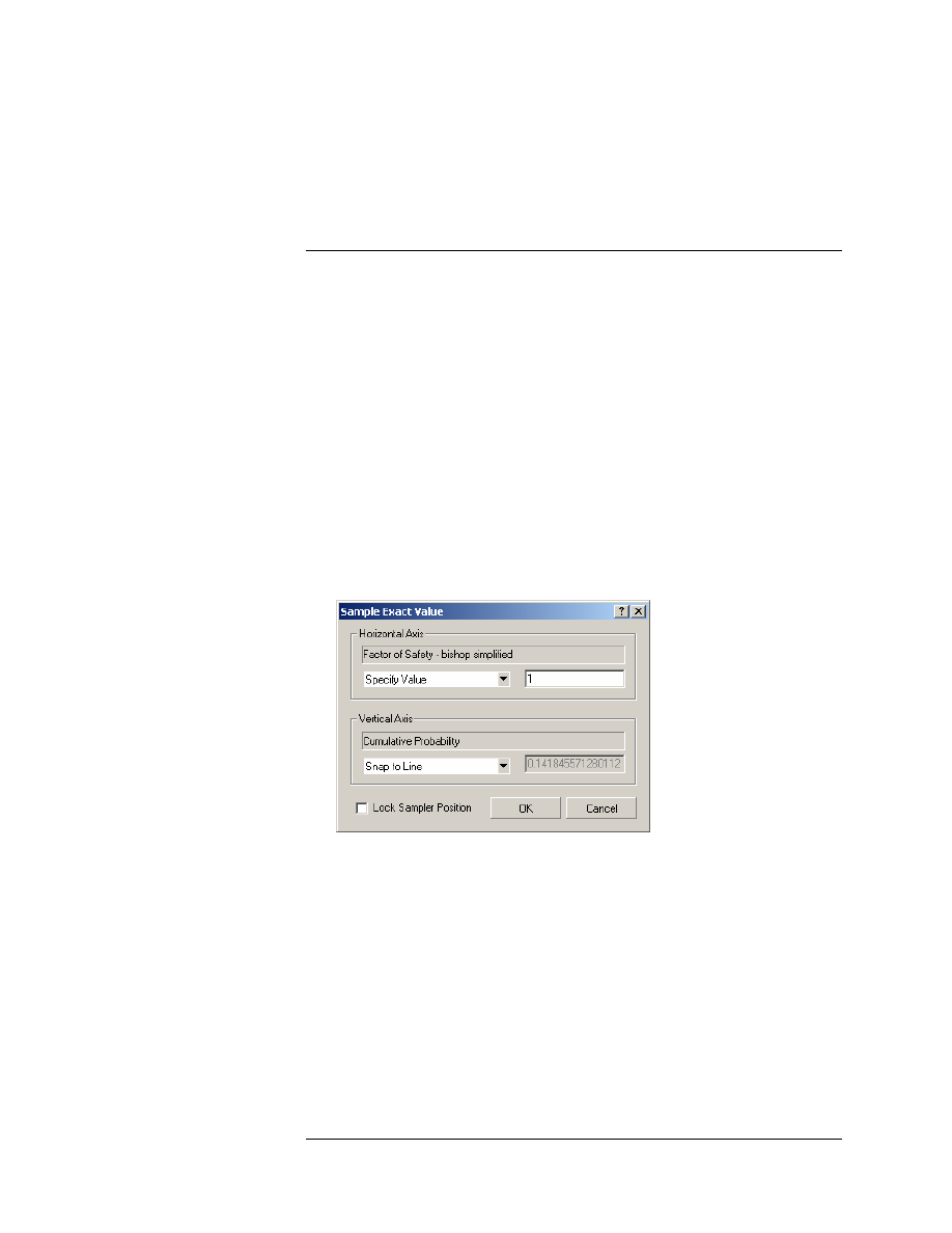
4. You can also determine exact points on the curve as follows. Right-

click on the plot, and select Sample Exact Value. You will see the

following dialog.

5. Enter 1 as the value for safety factor, and select OK.

6. Notice that the Sampler (dotted line) is now located at exactly Safety

Factor = 1. Also notice that the Cumulative Probability = 0.11. This

means that the Probability of Failure (Bishop analysis method) =

11%, which is the value we noted earlier in this tutorial, displayed at

the slip center of the Global Minimum slip surface.

Slide v.5.0 Tutorial

Manual

Probabilistic Analysis Tutorial

8-16

Scatter Plots

Scatter Plots allow you to plot any two random variables against each

other, on the same plot. This allows you to analyze the relationships

between variables.

Select the Scatter Plot option from the toolbar or the Statistics menu.

Select: Statistics

→ Scatter Plot

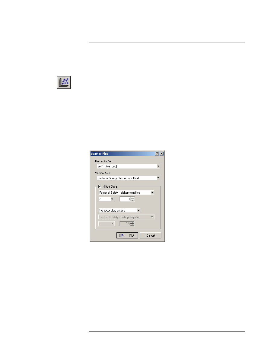
You will see the Scatter Plot dialog. Enter the following data.

1. Set the Horizontal Axis = soil 1 : Phi.

2. Set the Vertical Axis = Factor of Safety – Bishop.

3. Select Highlight Data, and select “Factor of Safety – Bishop

Simplified < 1”.

4. Select Plot.

You should see the following plot.

Slide v.5.0 Tutorial

Manual

Probabilistic Analysis Tutorial

8-17

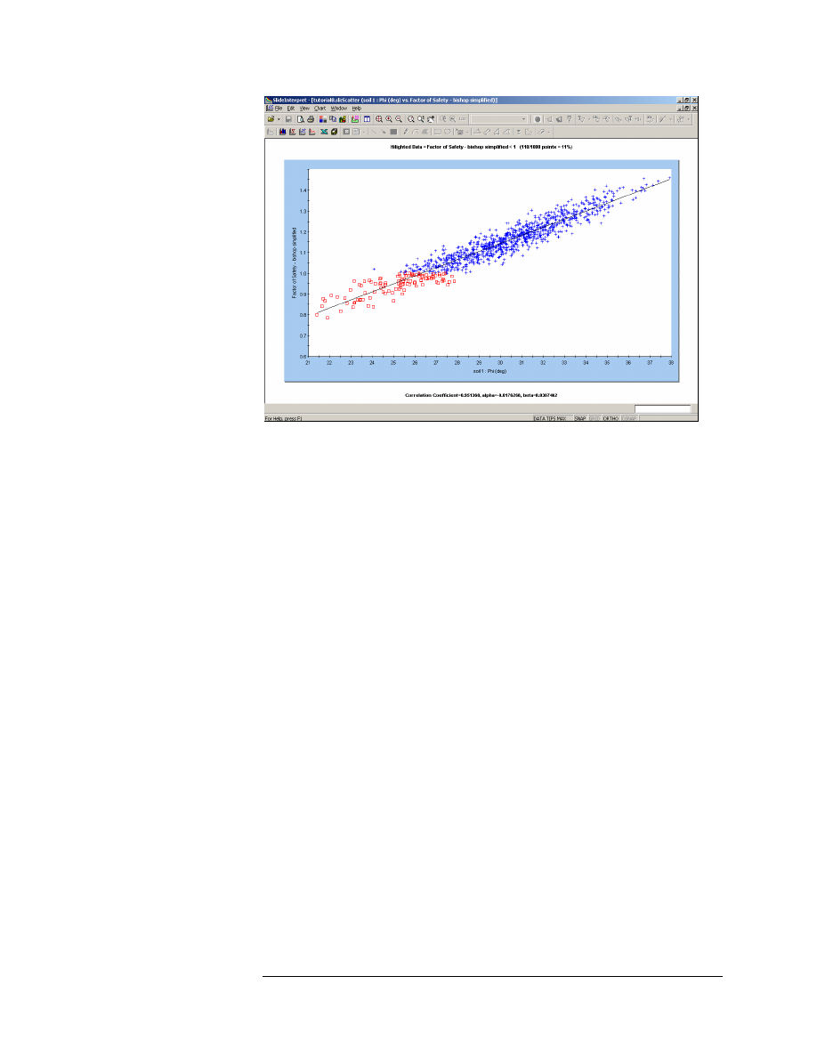
Figure 8-7: Scatter Plot – Friction Angle versus Safety Factor.

There is a well defined relationship between Friction Angle and Safety

Factor. Notice the parameters listed at the bottom of the plot.

• The Correlation Coefficient indicates the degree of correlation

between the two variables plotted. A Correlation Coefficient close to 1

(or -1) indicates a high degree of correlation. A Correlation Coefficient

close to zero, indicates little or no correlation.

• The parameters Alpha and Beta, are the slope and y-intercept,

respectively, of the best fit (linear) curve, to the data. This line can be

seen on the plot. Its display can be toggled on or off, by right-clicking

on the plot and selecting the Regression Line option.

Also notice the highlighted data on the plot. All data points with a Safety

Factor less than 1, are displayed on the Scatter Plot as a RED SQUARE,

rather than a BLUE CROSS.

Now let’s plot Phi versus Cohesion on the Scatter Plot.

Right-click on the plot and select Change Plot Data. On the Vertical Axis,
select soil 1 : Cohesion. Select Done. The plot should look as follows:

Slide v.5.0 Tutorial

Manual

Probabilistic Analysis Tutorial

8-18

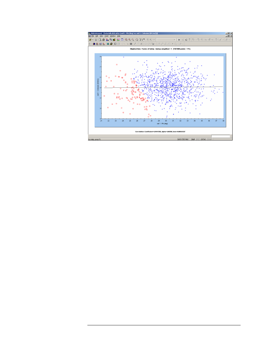
Figure 8-8: Scatter Plot – Friction Angle versus Cohesion.

This plot indicates that there is no correlation between the sampled

values of Cohesion and Friction Angle. (The Correlation Coefficient,

listed at the bottom of the plot, is a small number close to zero).

In reality, the Cohesion and Friction Angle of Mohr-Coulomb materials

are generally correlated, such that materials with low Cohesion often

have high Friction Angles, and vice versa.

In Slide, the user can define a correlation coefficient for Cohesion and

Friction Angle, so that when the samples are generated, Cohesion and

Friction Angle will be correlated. This is discussed at the end of this

tutorial.

Slide v.5.0 Tutorial

Manual

Probabilistic Analysis Tutorial

8-19

Convergence Plots

A Convergence Plot is useful for determining whether or not your

Probabilistic Analysis is converging to a final answer, or whether more

samples are required.

Select the Convergence Plot option from the toolbar or the Statistics

menu.

Select: Statistics

→ Convergence Plot

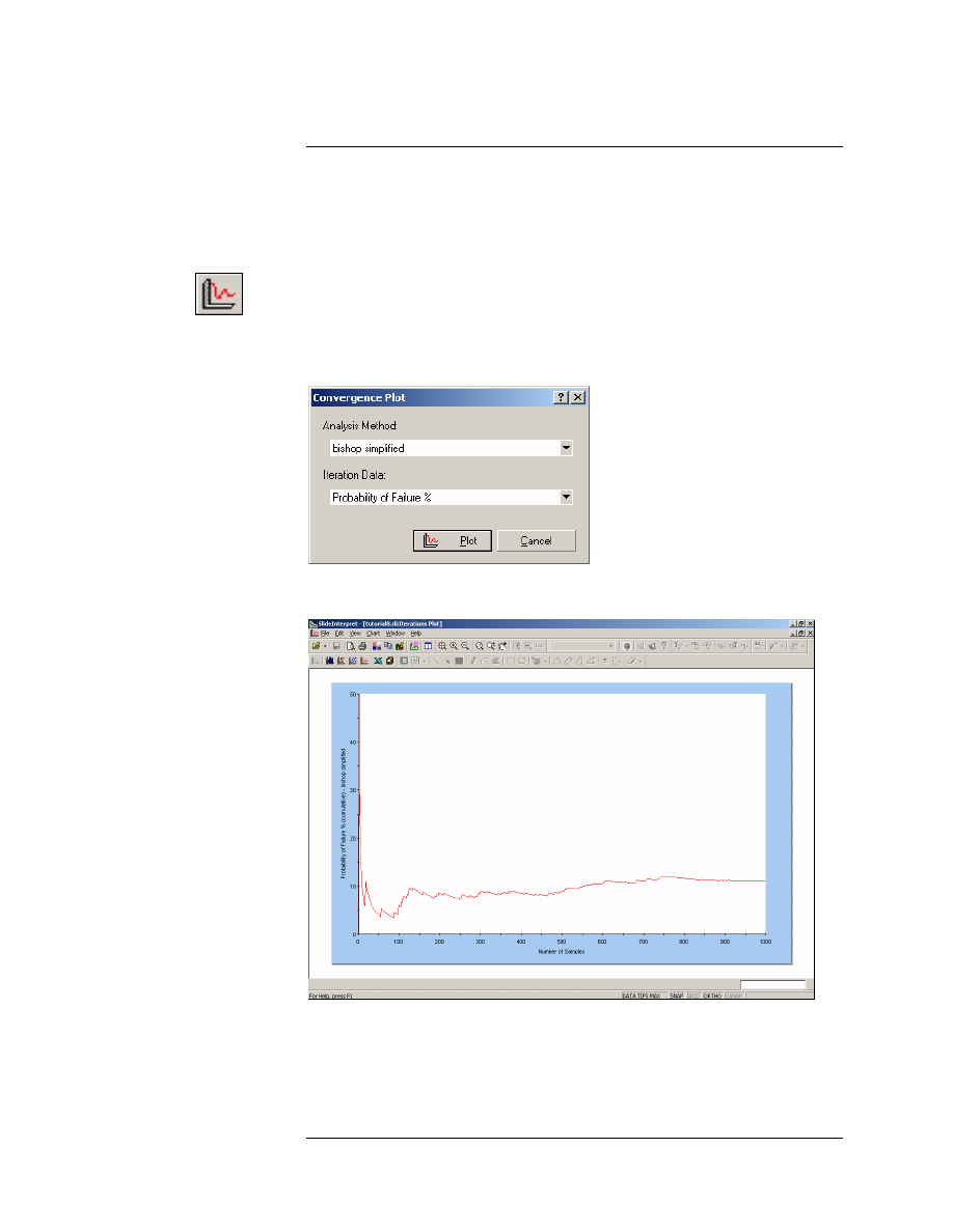
You will see the Convergence Plot dialog. Select Probability of Failure.
Select Plot.

You should see the following plot.

Figure 8-9: Convergence plot – Probability of Failure.

Slide v.5.0 Tutorial

Manual

Probabilistic Analysis Tutorial

8-20

A convergence plot should indicate that the final results of the

Probabilistic Analysis, are converging to stable, final values (i.e.

Probability of Failure, Mean Safety Factor etc.)

If the convergence plot indicates that you have not achieved a stable,

final result, then you should increase the Number of Samples, and re-run

the analysis.

Right-click on the plot and select the Final Value option from the popup

menu. A horizontal line will appear on the plot, which represents the

final value (in this case, Probability of Failure = 11%), which was

calculated for the analysis.

For this model, it appears that the Probability of Failure has achieved a

constant final value. To verify this, increase the Number of Samples (e.g.

2000), and re-run the analysis. This is left as an optional exercise.

Additional Exercises

The user is encouraged to experiment with the Probabilistic Analysis
modeling and data interpretation features in Slide. Try the following

exercises.

Correlation Coefficient (C and Phi)

Earlier in this tutorial, we viewed a Scatter Plot of Cohesion versus

Friction Angle (see Figure 8-8).

Because the random sampling of these two variables, was performed

entirely independently, there was no correlation between the two

variables.

In reality, the Cohesion and Friction Angle of Mohr-Coulomb materials

are generally correlated, such that materials with low Cohesion tend to

have high Friction Angles, and vice versa.

In Slide, the user can easily define a correlation coefficient for Cohesion

and Friction Angle, so that when the samples are generated, Cohesion

and Friction Angle will be correlated.

This can be demonstrated as follows:

1. In the Slide Model program, select the Material Statistics option in

the Statistics menu.

2. In the Material Statistics dialog, select the Correlation option. This

will display a dialog, which allows you to define a correlation

coefficient, between cohesion and friction angle (this is only

applicable for materials which use the Mohr-Coulomb strength type).

Slide v.5.0 Tutorial

Manual

Probabilistic Analysis Tutorial

8-21

3. In the correlation dialog, select the Apply checkbox for “soil 1”. We

will use the default correlation coefficient of –0.5. Select OK in the

Correlation dialog. Select OK in the Material Statistics dialog.

4. Re-compute the analysis.

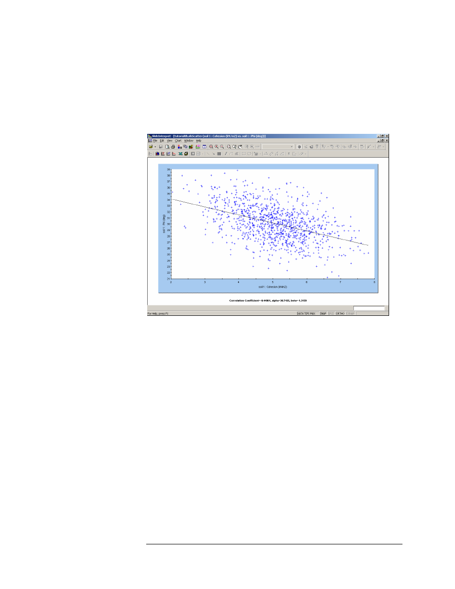
5. In the Slide Interpret program, create a Scatter Plot of Cohesion

versus Friction Angle. You should see the following.

Figure 8-10: Cohesion vs. Phi (Correlation = – 0.5).

As you can now see, Cohesion and Friction Angle are no longer

independent of each other, but are loosely correlated. NOTE:

• The actual correlation coefficient generated by the sampling, is listed

at the bottom of the plot. It is not exactly equal to – 0.5, because we

are using Monte Carlo sampling, and a relatively small number of

samples (1000).

• A NEGATIVE correlation coefficient simply means that when one

variable increases, the other is likely to decrease, and vice versa.

Now try the following:

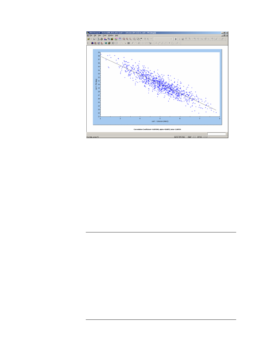
1. Re-run the analysis using correlation coefficients of – 0.6 , – 0.7, –

0.8 , – 0.9, – 1.0. View a scatter plot of Cohesion versus Friction

Angle, after each run.

2. You will see that the two variables will be increasingly correlated.

When the correlation coefficient = – 1.0, the Scatter Plot will result in

a straight line.

Slide v.5.0 Tutorial

Manual

Probabilistic Analysis Tutorial

8-22

Figure 8-11: Cohesion vs. Phi (Correlation = – 0.9).

In general, it is recommended that a correlation coefficient is defined

between Cohesion and Friction Angle, for a Mohr-Coulomb material. This

will generate values of Cohesion and Friction Angle, which are more

likely to occur in the field.

Finally, it is interesting to note that the Probability of Failure, for this

model, decreases significantly, as the correlation between cohesion and

friction angle increases (i.e. closer to –1).

This implies that the use of a correlation coefficient, and the generation

of more realistic combinations of Cohesion and Phi, tends to decrease the

calculated probability of failure, for this model.

Sampling Method

In this tutorial we used the default method of Random Sampling, known
as Monte Carlo Sampling. Another sampling method is available in Slide

– the Latin Hypercube method.

For a given number of samples, Latin Hypercube sampling results in a

smoother, more uniform sampling of the probability density functions

which you have defined for your random variables, compared to the

Monte Carlo method.

To illustrate this, do the following:

1. In the Slide Model program, select Project Settings > Statistics, and

set the Sampling Method to Latin Hypercube.

Slide v.5.0 Tutorial

Manual

Probabilistic Analysis Tutorial

8-23

2. Re-compute the analysis.

3. View the results in Interpret, and compare with the previous (Monte

Carlo) results. In particular, plot histograms of your input random

variables (Cohesion, Phi, Unit Weight).

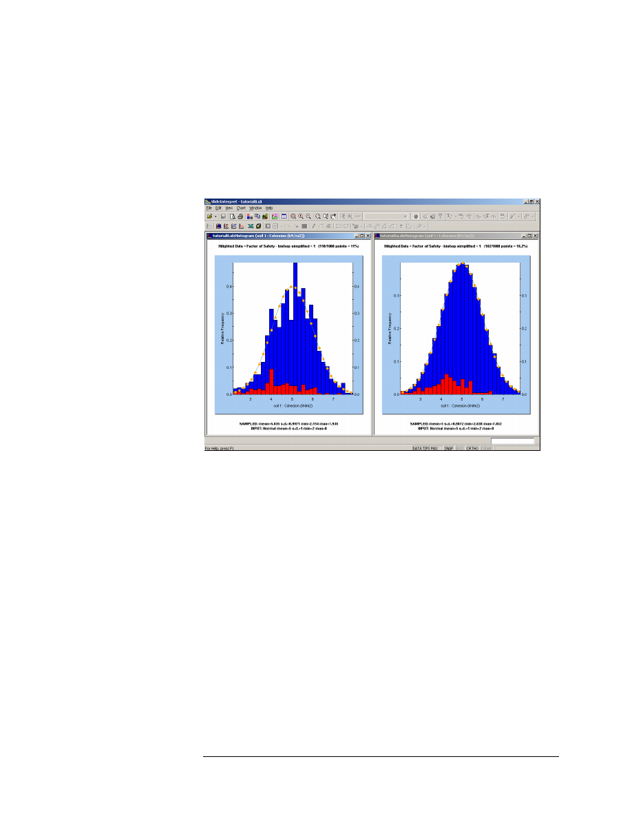
4. Notice that the input data distributions which you defined for your

input random variables, are much more smoothly sampled by Latin

Hypercube sampling, compared to Monte Carlo sampling.

Figure 8-12: Comparison of Monte Carlo sampling (left) and Latin Hypercube
sampling (right) – Cohesion random variable – 1000 samples.

As you can see in Figure 8-12, for 1000 samples, the Latin Hypercube

sampling is much smoother than the Monte Carlo sampling.

This is because the Latin Hypercube method is based upon "stratified"

sampling, with random selection within each stratum. Typically, an

analysis using 1000 samples obtained by the Latin Hypercube technique

will produce comparable results to an analysis of 5000 samples using the

Monte Carlo method.

In general, the Latin Hypercube method allows you to achieve similar

results to the Monte Carlo method, with a significantly smaller number

of samples.

Slide v.5.0 Tutorial

Manual

Probabilistic Analysis Tutorial

8-24

Slide v.5.0 Tutorial

Manual

Random Number Generation

The sampling of the statistical distributions of your input data random

variables, is achieved by the generation of random numbers. You may

wonder why the results in this tutorial are reproducible, if they are based

on random numbers?

The reason for this, is because we have been using the Pseudo-Random

option, in Project Settings. Pseudo-random analysis means that the same

sequence of random numbers is always generated, because the same

“seed” value is used. This allows the user to obtain reproducible results

for a Probabilistic Analysis.

Try the following:

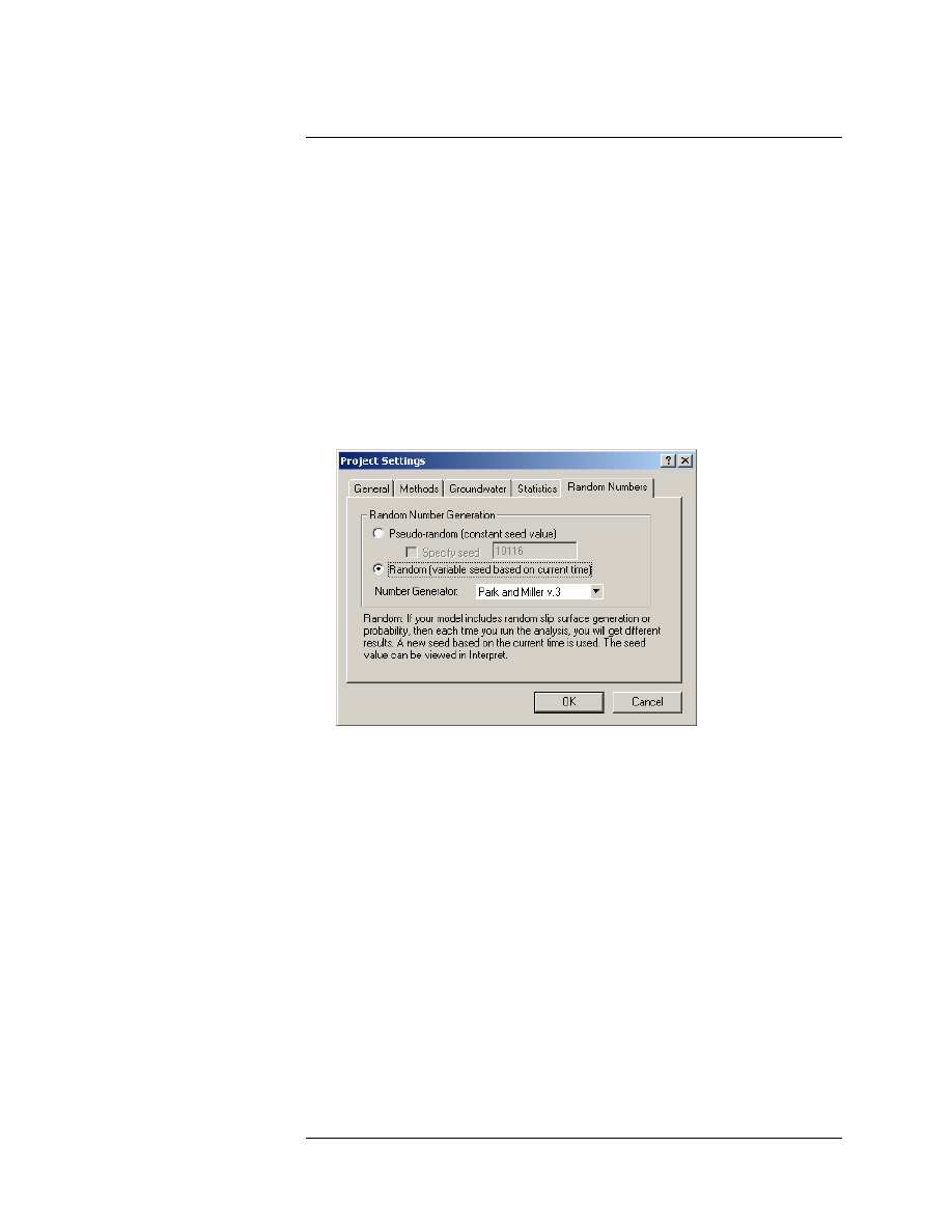
1. Select Project Settings > Random Numbers, and select the Random

option (instead of Pseudo-Random).

2. Re-compute the analysis.

3. You will notice that each time you re-compute, analysis results will

be different. This is because a different “seed” value is used each

time. This will give a different sequence of random numbers, and

therefore a different sampling of your random variables, each time

you re-run the analysis.

Document Outline