
Laplace Transform
•Pierre Simon de Laplace
•Oliver Heaviside
•Laplace transform definition
•Convergence region for Laplace
transform
•Laplace transform – analytic function
•Laplace transform examples
•Laplace transform properties
•Time differentiation
•Initial condition and value theorems
•Summary
„Signal Theory” Zdzisław Papir
Pierre Simone de
LAPLACE (
1749
-
†
1827)
Laplace was a mathematician and astronomer. Laplace
initially made an impact by
solving a complex problem of
mutual gravitation
that had eluded both Euler and
Lagrange. Laplace was among the most influential
scientists of his time and was called the Newton of France
for his study of and contributions to the
understanding of
the stability of the solar system
. Laplace generalized the
laws of mechanics for their application to the motion and
properties of the heavenly bodies. He is also famous for
his great treatises entitled
Mécanique céleste
and
Théorie
analytique des probabilités
. They were advanced in large
part by the mathematical techniques that Laplace
developed; most notably among those techniques are
generating functions, differential operators, and definite
integrals
.
„Signal Theory” Zdzisław Papir

Oliver HEAVISIDE
He then conducted private electrical research in a state of
near poverty. His views on
using inductance coils for
improving the performance of long-distance cables
ultimately proved correct. In 1901 he predicted the
existence of the ionosophere
. Heaviside formulated a
basis
for operational calculus
converting linear differential
equations into algebraic ones the solution of which can be
accomplished by relatively simple methods.
The Royal Society refused to publish his paper and Lord
Rayleigh once wrote to him „In the form, as it is, I am
afraid that your paper may not be of use to anyone”.
(
1850
- †
1925)
Oliver Heaviside, English mathematical physicist and
electrical engineer, made important contributions to
electromagnetic theory and measurement and anticipated
several advanced developments in mathematics and
electrical engineering. Heaviside had a brief career as
a telegrapher until growing deafness forced him to retire.
„Signal Theory” Zdzisław Papir

Laplace transform
definition
Fourier transform
dt
e
t
x
j
X
t
j
Laplace transform
0
0
signal)
(causal
0
for
0
dt
e
e
t
x
dt
e
t
x
s
X
j
s
t
t
x
t
j
t
st
„Signal Theory” Zdzisław Papir
t
x
s
X
dt
e
t
x
s
X
st
L
0

Laplace transform
definition – comment #1
0
0
signal)
(causal
0
for
0
dt
e
e
t
x
dt
e
t
x
s
X
j
s
t
t
x
t
j
t
st
Laplace transform
„Signal Theory” Zdzisław Papir
t
j
e
t
x
s
X
F
Laplace transform can be interpreted as a Fourier transform
of an original signal x(t) attenuated by an decaying
exponential term
exp(-j
t),
> 0
. Therefore, one can expect
that a broader class of signals is Laplace-transformable.

Laplace transform
definition – comment #2
0
0
signal)
(causal
0
for
0
dt
e
e
t
x
dt
e
t
x
s
X
j
s
t
t
x
t
j
t
st
Laplace transform
„Signal Theory” Zdzisław Papir
The lower limit in the Laplace integral allows for
inclusion any Dirac pulses
(t)
.

Inverse Laplace transform
s
X
t
x
ds
e
s
X
j
ds
e
s
X
j
t
x
j
j
st
j
j
st
1
-
L
lim
2
1
2
1
„Signal Theory” Zdzisław Papir
Laplace transform
definition – comment
#3
• An efficient method for obtaining the inverse Laplace
transform employs the
partial fraction expansion
of a Laplace transform being a
rational function
in s.
• Laplace transform without any
essential singularities
are rational function
in s.

Convergence region for
Laplace transform
0
,
1
0
0
a
a
j
j
X
j
a
e
dt
e
e
j
X
e
t
t
x
t
j
a
t
j
at
at
1
Fourier transform
„Signal Theory” Zdzisław Papir
Fourier transform
(integral) is
convergent for a < 0
only,
moreover, it is convergent on the imaginary
j
axis solely.
a
a
s
s
X
s
a
e
e
s
a
e
dt
e
e
s
X
e
t
t
x
t
j
t
a
t
s
a
st
at
at
,
1
0
0
0
1
Laplace transform
„Signal Theory” Zdzisław Papir
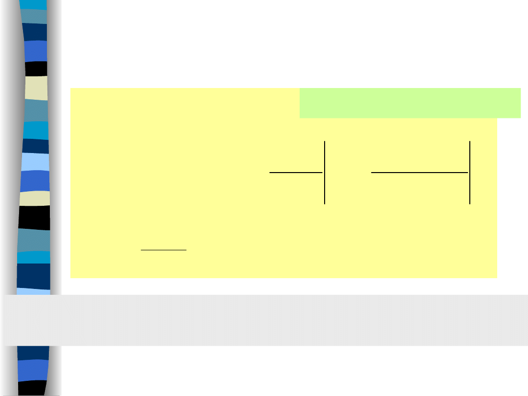
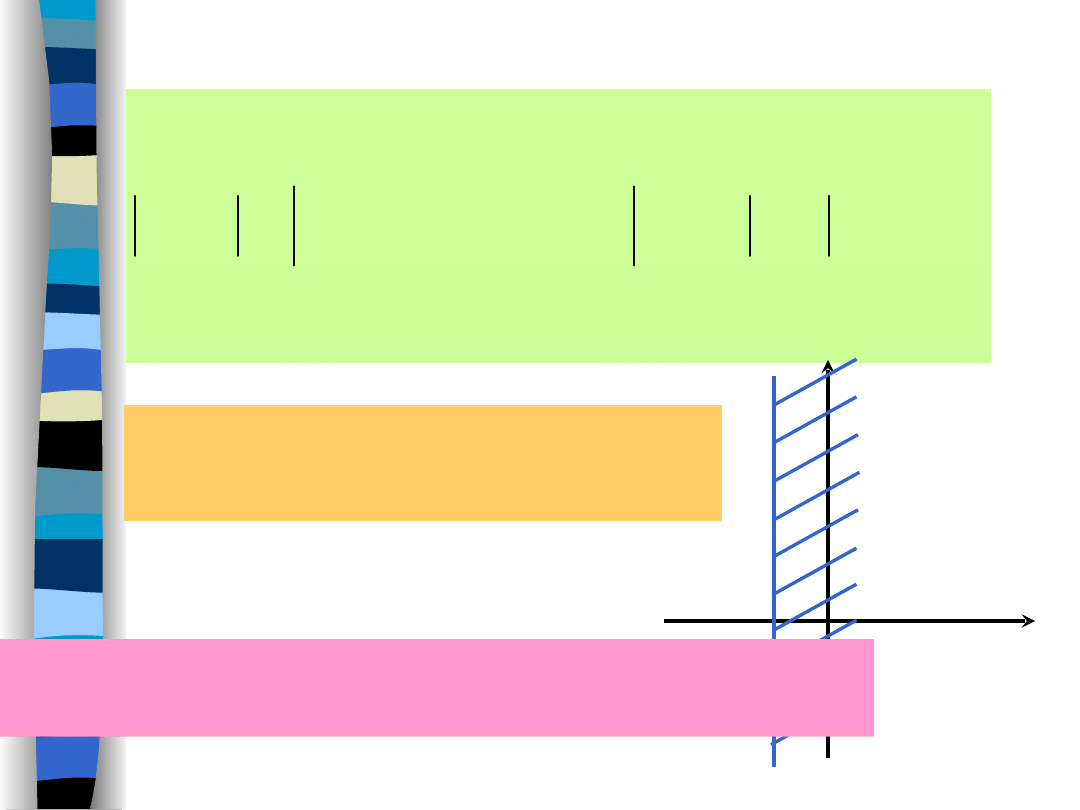
Convergence region for
Laplace transform
Laplace transform
(integral) is
convergent for any a
in a complex halfplane
Re
(s) =
> a.
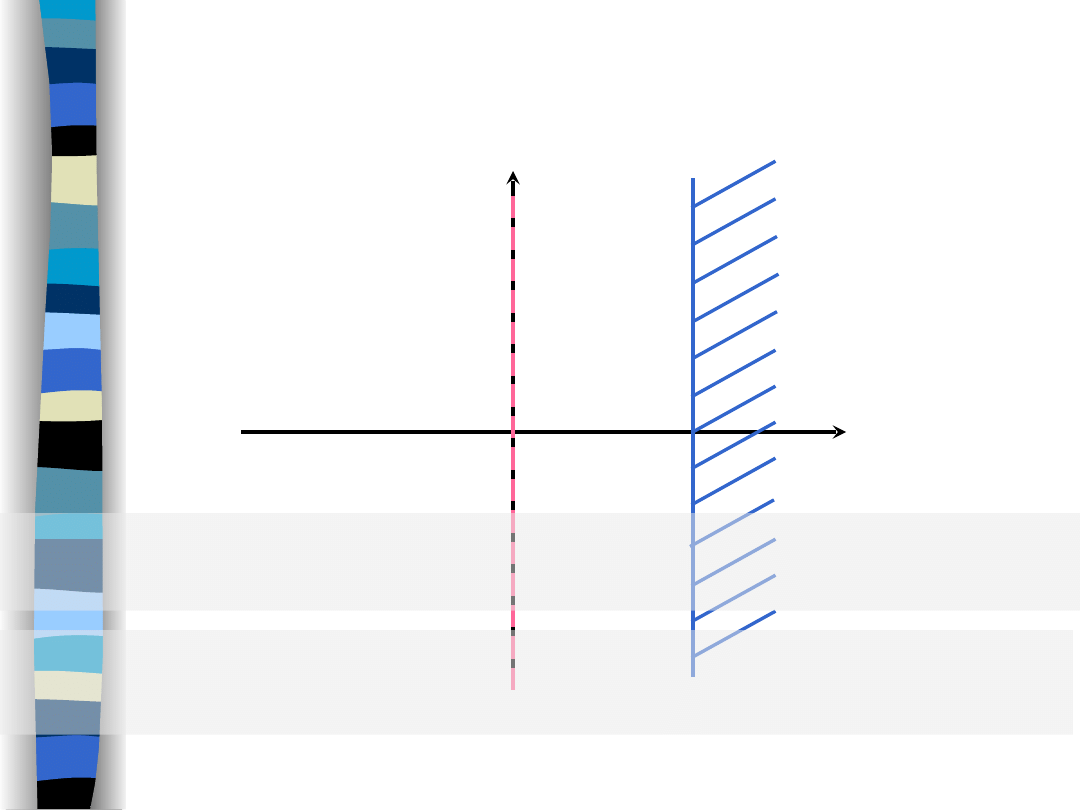
Convergence regions
compared
„Signal Theory” Zdzisław Papir
j
j
s
L
> a
a < 0
F
= 0
a
Fourier transform
(integral) is
convergent for a < 0
only,
moreover, it is convergent on the imaginary
j
axis solely.
Laplace transform
(integral) is
convergent for any a
in a complex halfplane
Re
(s) =
> a.
0
0
dt
e
e
t
x
dt
e
t
x
s
X
t
j
t
st
„Signal Theory” Zdzisław Papir
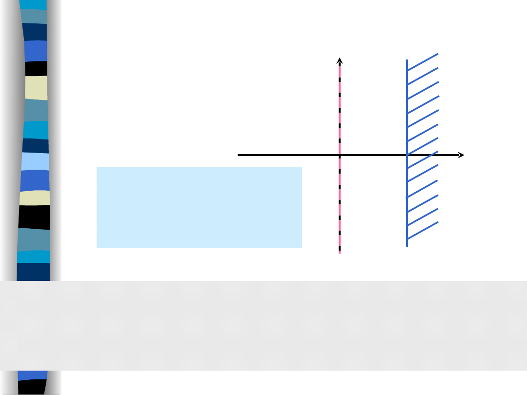
Convergence regions
compared
j
j
s
L
> a
a < 0
F
= 0
a
Laplace transform can be interpreted as a Fourier transform
of an original signal x(t) attenuated by an decaying
exponential term
exp(-j
t),
> 0
. As result,
a broader class of signals is Laplace-transformable.
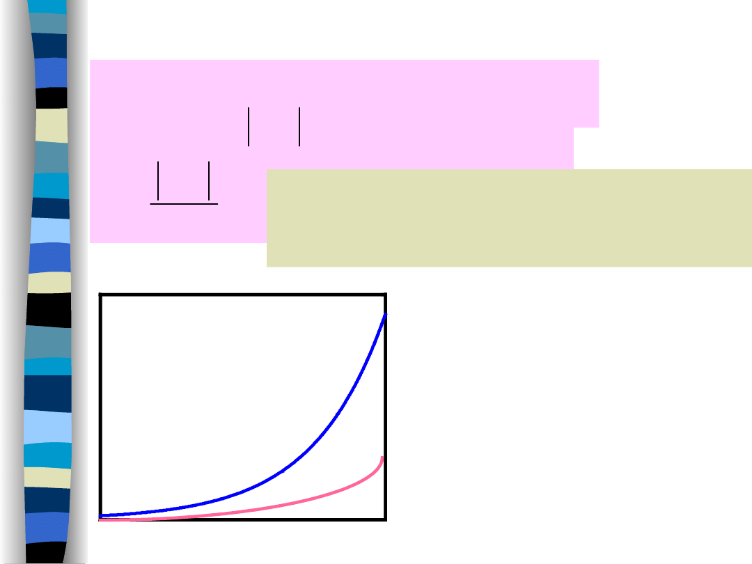
Exponential growth index
Signal x(t) is said to be of
exponential order if:
.
0
lim
for
:
0
,
t
t
t
Me
t
x
t
Me
t
x
M
Signal x(t) does not grow faster than
some exponential signal;
is called a
growth index of x(t).
t
Me
t
x
„Signal Theory” Zdzisław Papir
Convergence abscissa
0
0
0
0
0
0
dt
Me
dt
e
Me
dt
e
t
x
dt
e
e
t
x
s
X
dt
e
e
t
x
dt
e
t
x
s
X
t
t
t
t
t
j
t
t
j
t
st
0
a
dt
Me
t
j
j
s
L
>
< 0
Exponential growth index
Convergence abscissa
for Laplace transform.
„Signal Theory” Zdzisław Papir
Laplace transform
– analytic function
Function
C
f(s), s
C
is analytic if its derivative exists no
matter which path s is approaching s
0
.
0
0
0
0
lim
s
s
s
X
s
X
s
X
s
s
j
j
s
0
s
„Signal Theory” Zdzisław Papir
Laplace transforms
are
analytic functions
(for
Re
s
) so
important results are valid based on a
complex function
analysis
.
Cauchy integral theorem
L
0
ds
s
X
j
j
s
L
L
„Signal Theory” Zdzisław Papir
Laplace transform
– analytic function – Cauchy
theorem
j
j
s
L
Cauchy integral formula
L
ds
s
s
s
X
j
s
X
0
0
2
1
Value of an analytic function in any point s
0
L can be determined
if its values on an area boundary L are known.
L
0
s
„Signal Theory” Zdzisław Papir
Laplace transform
– analytic function – Cauchy
formula

Laplace transform
examples
a
s
e
s
t
s
n
t
s
t
s
s
t
at
n
n
t
t
t
t
t
1
1
1
!
sin
cos
1
2
0
2
0
0
2
0
2
0
1
1
1
1
1
„Signal Theory” Zdzisław Papir
Some signals that are not Fourier-transformable
(in an ordinary sense) are Laplace-transformable.

Laplace transform
properties
0
,
0
a
s
X
e
a
t
x
s
Y
s
X
t
y
t
x
a
s
X
t
x
e
s
s
X
d
x
a
a
s
X
at
x
s
bY
s
aX
t
by
t
ax
as
at
t
„Signal Theory” Zdzisław Papir
Laplace transform properties are similar
to Fourier transform properties; the difference is
in convergence regions.

Time differentiation
s
sX
x
e
x
dt
e
t
x
s
e
t
x
dt
e
t
x
t
x
Me
x
s
s
X
st
st
st
0
lim
as
,
0
0
0
0
L
0
x
s
sX
t
x
L
„Signal Theory” Zdzisław Papir
Time differentiation is a significant property as it replaces
differentiation in the time domain
to an
ordinary multi-
plication by s
in the complex frequency domain.

Time differentiation
0
0
0
0
0
0
2
3
2
x
x
s
x
s
s
X
s
t
x
x
x
s
s
X
s
t
x
x
s
sX
t
x
L
L
L
Time differentiation is quite significant property as:
• differential equations can be solved using
algebraic techniques
(d()/dt operator is replaced
by s-operator),
•
initial conditions
are included automatically,
• initial values and initial conditions have not to be
distinguished
(initial/final value theorem)
.
„Signal Theory” Zdzisław Papir

Time differentiation
(Fourier transform)
j
X
j
x
e
x
dt
e
t
x
j
e
t
x
dt
e
t
x
t
x
x
j
j
X
t
j
t
j
t
j
0
lim
0
for
,
0
0
0
0
F
Fourier transform
makes
algebraic solving differential
equations possible as well, however:
• assumptions are more restrictive
• is not convenient as consecutive derivative operators are:
(j
, -
2
, -j
3
,
4
...) as opposed to the Laplace transform
(s, s
2
, s
3
, s
4
, s
5
...).
„Signal Theory” Zdzisław Papir
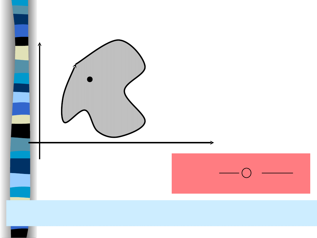
Initial condition
& value theorems
x(t)
t
continuous signal
discontinuous signal
x(0–)
x(0+)
x(0–) = x(0+) = x(0)
x(0–) –
initial
condition
x(0+) –
initial
value
„Signal Theory” Zdzisław Papir
Initial conditions can differ from initial values
when:
• signal driving an electric network changes stepwise
• electric network structure is subjected to a change
of its structure and was not deenergized right before.

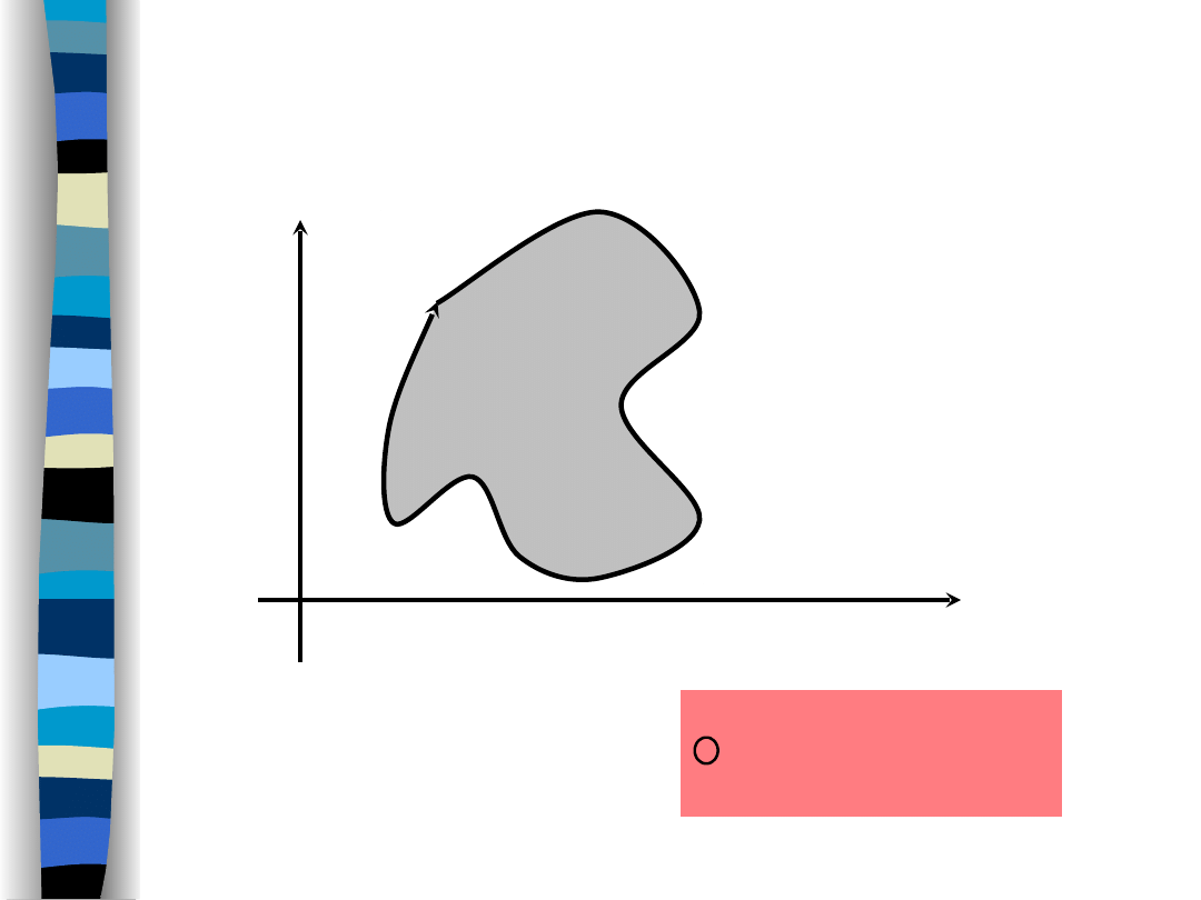
Initial value theorem
„Signal Theory” Zdzisław Papir
Consider a signal x(t) either continuous or
having
a finite discontinuity
at t = 0.
s
sX
x
t
x
s
X
t
x
s
t
lim
0
lim
0
The
initial value theorem
emphasizes the fact
that the
initial value
of a signal is to be determined
from
knowledge of its transform
(no matter if there is
a discontinuity x(0–) x(0+) at t = 0).

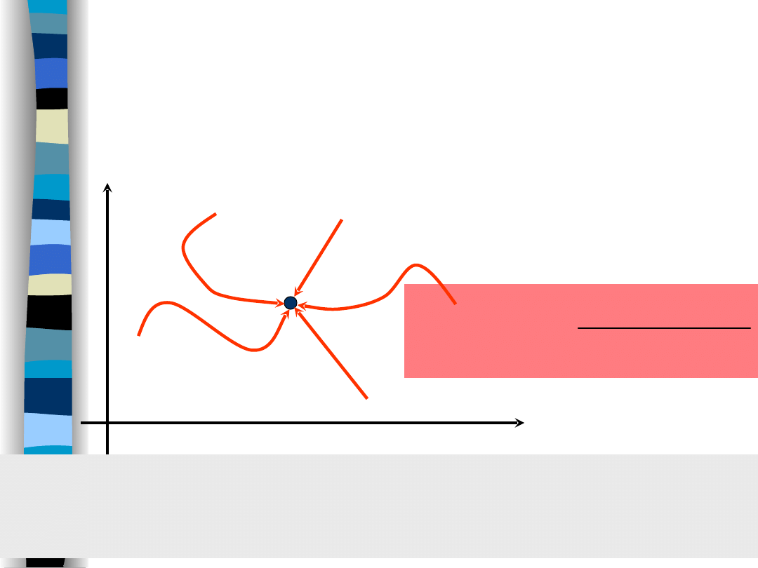
Final value theorem
„Signal Theory” Zdzisław Papir
Let the Laplace transform x(t) X(s) be analytic
in a right halfplane (
Re
s 0)
s
sX
t
x
s
X
t
x
s
t
0
lim
lim
The
final value theorem
emphasizes the fact
that the
steady state value
of a signal is to be determined
from
knowledge of its transform
.
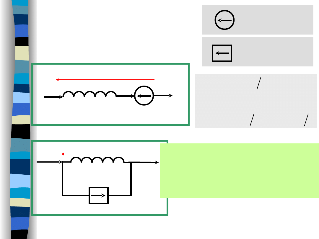
Initial condition
(an inductor)
Voltage source
„Signal Theory” Zdzisław Papir
Current source
s
i
Ls
s
U
s
I
Li
s
LsI
s
U
dt
t
di
L
t
u
0
0
Li(0–)
Ls
I(s)
U(s)
1/Ls
i(0–)/s
U(s)
I(s)
Initial energy storage in
an inductor is accounted for
by additional equivalent
sources (voltage/current).
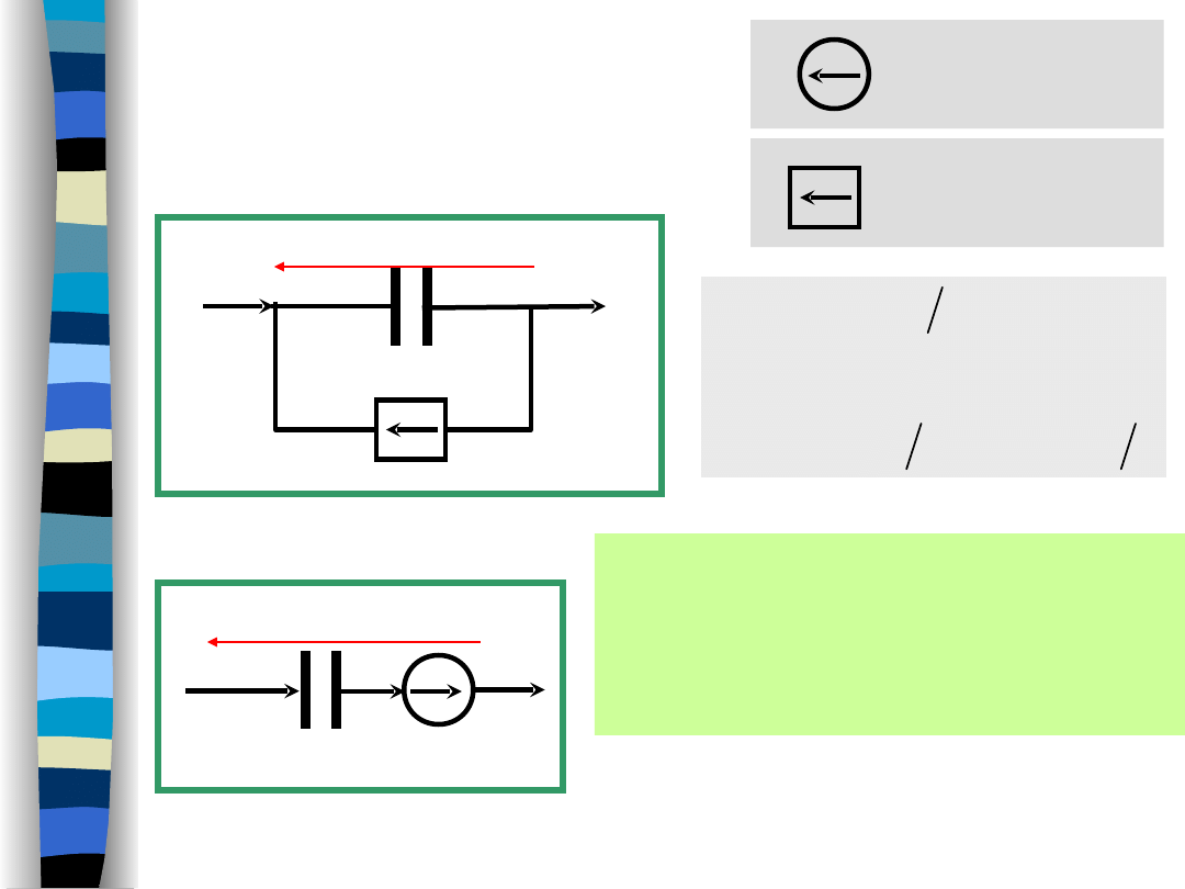
Initial condition
(a capacitor)
„Signal Theory” Zdzisław Papir
Voltage source
Current source
s
u
Cs
s
I
s
U
Cu
s
CsU
s
I
dt
t
Cdu
t
i
0
0
Initial energy storage in
an inductor is accounted for
by additional equivalent
sources (voltage/current).
Cs
Cu(0–)
I(s)
U(s)
u(0–)/s
1/Cs
I(s)
U(s)
t
L
R
A
t
i
t
R
U
t
i
exp
T
F
1
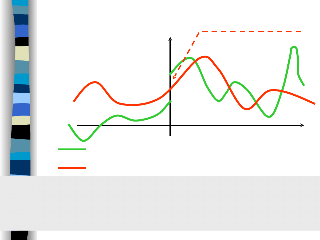
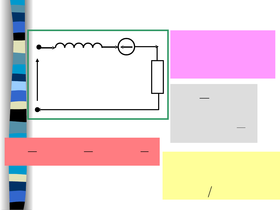
Example (a classic
approach)
R
U
I
A
I
i
i
i
i
A
i
0
0
F
T
)
0
(
)
0
(
0
0
0
t
L
R
t
R
U
I
t
R
U
t
i
exp
0
1
1
Li(0–) =
LI
0
L
t
U
1
R
i(t)
response
transient
-
response
forced
-
T
F
T
F
t
i
t
i
t
i
t
i
t
i
„Signal Theory” Zdzisław Papir
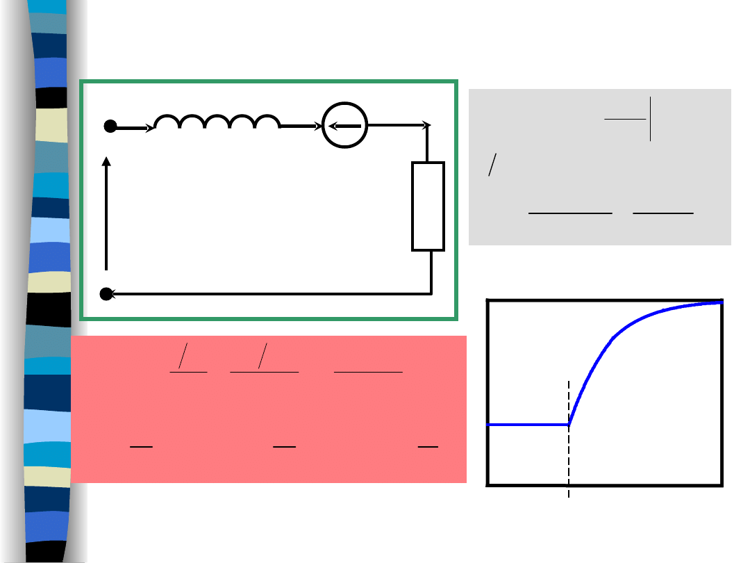
Example (Laplace
transform)
Ls
R
LI
Ls
R
s
U
s
I
LI
s
LsI
s
RI
s
U
dt
t
di
L
t
Ri
t
u
0
0
L
t
L
R
t
R
U
I
t
R
U
t
i
Ls
R
LI
Ls
R
R
L
s
R
U
s
I
exp
1
0
0
1
1
Li(0–) =
LI
0
L
t
U
1
R
i(t)
„Signal Theory” Zdzisław Papir
t = 0
t
I
0
i(t)
U/R

Summary
• Laplace transform is a convenient tool for solving
models of linear,
time-invariant systems (a set of fixed coefficients,
ordinary differential equations) as:
- it replaces the d()/dt operator by an algebraic s-
operator,
- yields a full solution comprising of a decaying
transient response (to initial conditions) and a forced
response (to external excitations).
• Class of Laplace-transformable signals is broader
than a class
Fourier-transformable signals due to a attenuating
term in the Laplace
transform kernel.
• Laplace transform are analytic functions (from
complex function analysis point of view) so we are
supported by a powerful technical apparatus (most
spectacular result are Hilbert relationships).
Telecommunication signals modeling is interested in a steady state in
most cases, therefore, more emphasis has been placed on the Fourier
transform which is more easy for a physical interpretation.
„Signal Theory” Zdzisław Papir
Document Outline
- Slide 1
- Slide 2
- Slide 3
- Slide 4
- Slide 5
- Slide 6
- Slide 7
- Slide 8
- Slide 9
- Slide 10
- Slide 11
- Slide 12
- Slide 13
- Slide 14
- Slide 15
- Slide 16
- Slide 17
- Slide 18
- Slide 19
- Slide 20
- Slide 21
- Slide 22
- Slide 23
- Slide 24
- Slide 25
- Slide 26
- Slide 27
- Slide 28
- Slide 29
Wyszukiwarka
Podobne podstrony:
Laplace Transform
Laplace Transforms and Inverse Laplace Transforms
Laplace Transforms and Inverse Laplace Transforms
New Laplace Transform Table
Fourier tranform and Laplace transfrom
Obliczanie transformat Laplace'a
Transformaty Laplacka
Transformata Laplacea oryginaly i transformaty funkcji [tryb zgodności]
AM23 w13 Transformata Laplace'a
Transformaty Laplace a
Transformacja Laplace wyprowadzenie wzorów
9 transformata Laplace'a + Transmitancja Operatorowa
Transformacja Laplacea
AM23 w14 Zastosowania transformaty Laplace'a
transformaty Laplace'a
Podstawowe regu y transformacji Laplace's (wzory)
transformata Laplaca
Transformata Laplace, Studia, Semestr 1, Sygnały i Systemy, Sprawozdanie 4
więcej podobnych podstron