
Przekształcenie Laplace’a
czyli
zaczynamy ułatwiać sobie życie
Przekształcenie Laplace’a
Rozważmy dowolną funkcję (dystrybucję)
f(t). Transformatą
Laplace’a f(t) nazywa się następujące przekształcenie całkowe
( )
{ }
( )
( )
0
e
d
st
f t
f t
t
F s
∞
−
−
=
∫
≜
L
gdzie
jest zespolonym parametrem przekształcenia,
j
s
σ
ω
= +
gdzie
jest zespolonym parametrem przekształcenia,
nazywanym zespoloną pulsacją.
Obszar
S
na płaszczyźnie
zespolonej nazywa się obszarem zbieżności transformaty Laplace’a,
jeżeli dla każdego
całka Laplace’a jest zbieżna.
j
s
σ
ω
= +
s
∈
S
Obszar zbieżności jest niepusty, jeżeli f(t) jest funkcją typu
wykładniczego, tzn.
( )
0
e
t
M
t
f t
M
ρ
ρ
>
<
∨∨∧

Odwrotne przekształcenie Laplace’a
Wzór Riemanna-Mellina
( )
{
}
( )
( )
+j
1
j
1
e d
2πj
c
st
c
F s
F s
s
f t
∞
−
− ∞
=
=
∫
L
Z wzoru Riemanna-Mellina otrzymuje się funkcję przyczynową
( )
0
dla
0.
f t
t
≡
<
Z wzoru Riemanna-Mellina otrzymuje się funkcję przyczynową
( )
( )
( )
{ }
( )
{
}
( )
( )
1
2
1
2
1
2
Jeżeli
0
i
0
dla
0
to
f t
f
t
t
f t
f
t
f t
f
t
≡
≡
<
=
⇔
=
L
L
Twierdzenie o jednoznaczności przekształcenia Laplace’a

( )
{ }
( )
( )
{
}
( )
1
f t
F s
F s
f t
−
=
⇔
=
L
L
f(t) — oryginał
F(s) — transformata
Stosuje się również oznaczenie
( )
( )
f t
F s
⇌
Przykład 1.
( ) ( )
( )
( )
( )
0
δ
δ
e
d
1
δ
1
st
f t
t
F s
t
t
t
∞
−
−
=
=
=
∫
⇌

Przykład 2.
( )
( )
( )
( )
( )
(
)
( )
(
)
( )
(
)
0
0
0
0
e
,
e
e
d
e
d
1
1
e
δ
e
d
at
s a t
at
st
s a t
s a t
f t
t
a
F s
t
t
t
t
t
t
t
s
a
s
a
∞
∞
− −
−
−
−
∞
∞
− −
− −
−
−
=
∈
=
=
=
= −
+
−
−
∫
∫
∫
1
1
1
1
ℝ
0
0
−
−
Całka będzie zbieżna, gdy Re{s – a} > 0. Wówczas
( )
( )
1
1
e
at
F s
s
a
t
s
a
= −
−
1
⇌
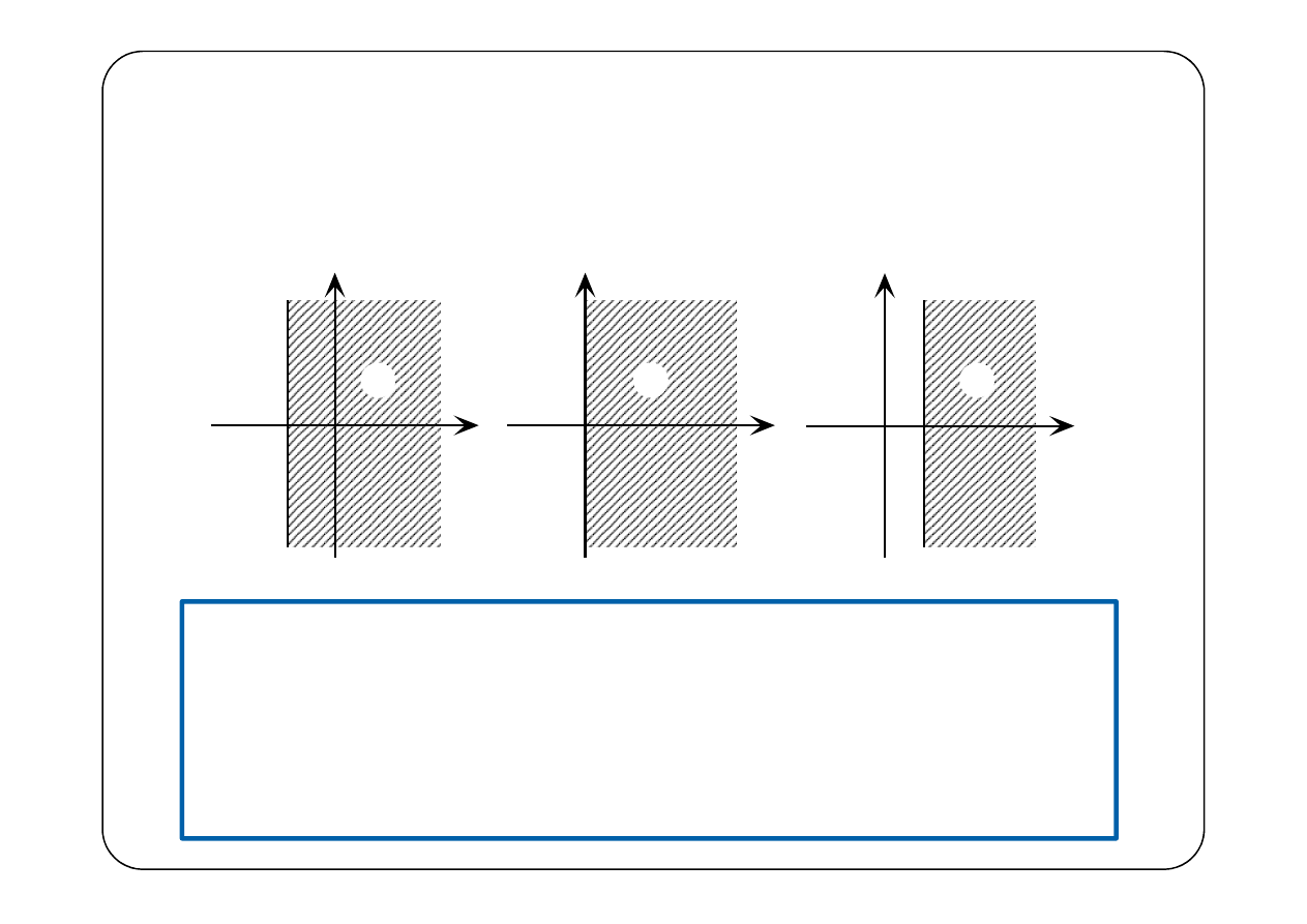
Obszarem zbieżności S na płaszczyźnie zespolonej jest
półpłaszczyzna Re{s} =
σ
> a
j
ω
σ
a
j
ω
σ
a
j
ω
σ
a
S
S
S
0
a
<
0
a
=
0
a
>
Jeżeli f(t) jest funkcją typu wykładniczego, to obszar
zbieżności transformaty Laplace’a S jest półpłaszczyzną
Re{s} >
σ
0
.
σ
0
nazywa się odciętą zbieżności transformaty
Laplace’a. W szczególności może zachodzić
σ
0
→
–
∞
, czyli
obszarem zbieżności jest cała płaszczyzna zespolona.

Twierdzenie
Transformata
jest w obszarze zbieżności S (czyli w półpłaszczyźnie Re{s} >
σ
0
)
funkcją holomorficzną, tzn. w każdym punkcie tego obszaru istnieje
pochodna
( )
( )
{ }
F s
f t
=
L
( )
( )
d
e
d .
st
F s
t f t
t
∞
−
= −
∫
( )
( )
0
e
d .
d
st
t f t
t
s
−
−
= −
∫
W praktycznych przypadkach funkcji f(t), reprezentującej przebieg
fizyczny, jej transformata poza obszarem zbieżności może mieć co
najwyżej przeliczalny zbiór odosobnionych punktów osobliwych,
którymi mogą być jedynie osobliwości usuwalne lub bieguny.
Funkcja taka nazywa się funkcją meromorficzną.

( )
( )
( )
( )
(
)
(
)
0
0
0
pod warunkiem, że
e
,
e
e
d
e
d
1
1
e
,
at
s a t
at
st
s a t
f t
t
a
F s
t
t
t
s
a
s
a
∞
∞
− −
−
+
+
∞
− −
+
=
∈
=
=
=
= −
=
−
−
∫
∫
1
1
ℝ
{ }
pod warunkiem, że
Re
.
s
a
>
Wniosek:
Jeżeli f(t) jest funkcją (nie zawiera składników dystrybucyjnych), to
jako dolną granicę całkowania można przyjąć zarówno 0– jak i 0+.

Własności przekształcenia Laplace’a
Stosować będziemy oznaczenia
( )
( )
( )
( )
,
f t
F s
g t
G s
⇌
⇌
1. Liniowość
( )
( )
( )
( )
1
2
1
2
a f t
a g t
a F s
a G s
+
+
⇌
2. Przesunięcie w dziedzinie s
( )
(
)
e
,
t
f t
F s
ξ
ξ
ξ
−
−
⇌
dowolna liczba
(rzeczywista, zespolona, urojona)
( )
{
}
( )
( )
(
)
(
)
0
0
e
e
e
d
e
d
s
t
t
t
st
f t
f t
t
f t
t
F s
ξ
ξ
ξ
ξ
∞
∞
− −
−
−
−
=
=
=
−
∫
∫
L
Dowód:

3. Różniczkowanie (dystrybucyjne) oryginału
( )
( )
( ) ( )
d
0
d
f t
f t
sF s
f
t
′
=
−
−
⇌
Dowód:
( )
{
}
( )
( )
( )
(
)
( )
( )
0
e
d
st
f
t
f
t
t
∞
−
−
∞
∞
−
−
′
′
=
=
=
−
−
= −
− +
∫
∫
L
( )
( )
(
)
( )
( )
0
0
e
e
d
0
st
st
f t
f t
s
t
f
sF s
∞
−
−
−
−
=
−
−
= −
− +
∫
4. Całkowanie (dystrybucyjne) oryginału
( )
( )
0
1
d
t
f
F s
s
τ τ
−
∫
⇌

5. Przesunięcie w dziedzinie t
(
) (
)
( )
0
0
0
e
st
f t
t
t
t
F s
−
−
−
1
⇌
Dowód:
(
) (
)
{
}
(
)
( )
(
)
( )
( )
0
0
0
0
0
0
0
0
0
e
d
e
d
e
e
d
e
s x t
st
t
st
st
sx
f t
t
t
t
f t
t
t
f x
x
f x
x
F s
∞
∞
−
+
−
∞
−
−
−
−
−
=
−
=
=
=
=
∫
∫
∫
1
L
6. Różniczkowanie transformaty
6. Różniczkowanie transformaty
( )
( )
d
d
t f t
F s
s
−
⇌
( )
( )
( )
( )
( )
{
}
0
0
0
d
d
e
d
e
d
d
d
e
d
st
st
st
F s
f t
t
f t
t
s
s
s
t f t
t
t f t
∞
∞
−
−
−
−
∞
−
−
∂
=
=
=
∂
=
−
= −
∫
∫
∫
L
Dowód:

7. Skalowanie
( )
( )
1
,
0
s
f at
F
a
a
a
>
⇌
8. Splot w dziedzinie t
( ) ( )
( ) (
)
( ) ( )
0
d
t
f t
g t
f
g t
F s G s
τ
τ τ
+
−
∗
=
−
∫
⇌
Dowód (szkic):
Dowód (szkic):
( ) ( )
{
}
( ) (
)
( ) (
)
( )
( )
( )
( ) ( )
0
0
0 0
0
0
d
e
d
e
e
d d
e
d
e
d
st
s t
s
s
s
f t
g t
f
g t
t
f
g t
t
f
g
F s G s
τ
τ
τ
ζ
τ
τ τ
τ
τ
τ
τ
τ
ζ
ζ
∞
∞
−
−
−
∞ ∞
−
−
−
− −
∞
∞
−
−
−
−
∗
=
−
=
=
−
=
=
=
∫ ∫
∫ ∫
∫
∫
L

8. Mnożenie funkcji w dziedzinie t
( ) ( )
( ) ( )
( ) (
)
j
j
1
1
d
2πj
2πj
c
c
f t g t
F s
G s
F
G s
λ
λ λ
+ ∞
− ∞
∗
=
−
∫
⇌

Transformaty elementarnych funkcji
( )
δ
1
t ⇌
( )
1
t
s
1
⇌
( )
1
e
at
t
s
a
−
+
1
⇌
( )
1
t
t
1
⇌
( )
2
1
t
t
s
1
⇌
(
) ( )
1
1
1 !
n
n
t
t
n
s
−
−
1
⇌
( )
0
0
2
2
0
sin
t
t
s
ω
ω
ω
⋅
+
1
⇌
( )
0
2
2
0
cos
s
t
t
s
ω
ω
⋅
+
1
⇌

Przykład 1.
( ) ( )
( )
3
1 e
t
f t
t
t
−
= −
1
( )
( )
( )
( )
( )
( )
(
)
3
3
3
3
2
e
e
1
e
3
d
1
1
e
d
3
3
t
t
t
t
f t
t
t
t
t
s
t
t
s s
s
−
−
−
−
=
−
+
−
=
+
+
1
1
1
1
⇌
⇌
( )
( )
{ }
(
)
(
)
2
2
1
1
2
3
3
3
s
F s
f t
s
s
s
+
=
=
−
= −
+
+
+
L
Inaczej
( ) ( )
( ) ( )
(
)
(
)
(
)
2
2
3
2
2
1
1
1
1
1
3
2
e
1
3
3
t
s
t
t
s
s
s
s
s
t
t
s
s
−
−
−
− =
− +
+
−
= −
+
+
1
1
⇌
⇌

Przykład 2.
( )
(
) ( )
2
e
cos3
2sin 3
t
f t
t
t
t
−
=
−
1
( )
( )
(
)
( )
2
2
2
cos 3
9
2
e
cos 3
2
9
3
sin 3
t
s
t
t
s
s
t
t
s
t
t
−
⋅
+
+
⋅
+
+
⋅
1
1
1
⇌
⇌
⇌
( )
( )
(
)
2
2
2
3
sin 3
9
3
e
sin 3
2
9
t
t
t
s
t
t
s
−
⋅
+
⋅
+
+
1
1
⇌
⇌
( )
( )
{ }
(
)
(
)
2
2
2
2
3
4
2
4
13
2
9
2
9
s
s
F s
f t
s
s
s
s
+
−
=
=
−
=
+
+
+
+
+
+
L
Przykład 3.
( )
(
) ( )
0
2 sin
f t
F
t
t
ω
θ
=
+ ⋅
1
( )
( )
( )
0
0
2 cos sin
2 sin cos
f t
F
t
t
F
t
t
θ
ω
θ
ω
=
⋅
+
⋅
1
1
( )
( )
{ }
0
2 cos
2 sin
s
F s
f t
F
F
ω
θ
θ
=
=
+
=
L
( )
( )
{ }
(
)
0
2
2
2
2
0
0
0
2
2
0
2 cos
2 sin
2
cos
sin
s
F s
f t
F
F
s
s
F
s
s
ω
θ
θ
ω
ω
ω
θ
θ
ω
=
=
+
=
+
+
+
=
+
L

Przykład 4.
( )
( )
3
1
f t
t
t
=
−
1
( )
( ) ( ) ( )
( )
( )
( ) ( )
( )
( )
{ }
( ) ( )
( )
( )
3
3
2
2
3
4
3
2
4
1
1
3
3
6
3 2
3
1
6 6
3
1
e
s
t
f t
t
t
t
t
t
t
t
t
t
s
s
s
s
t
s
s
s
s
s
f t
t
F s
s
ϕ
Φ
ϕ
ϕ
Φ
−
=
+ = +
=
+
+
+
⋅
+ +
+
=
=
+
+
+ =
=
−
⇒
=
1
1
1
1
1
L
( ) ( )
( )
( )
1
e
s
f t
t
F s
s
ϕ
Φ
−
=
−
⇒
=
( )
( )
{ }
2
3
4
6
6
3
e
s
s
s
s
F s
f t
s
−
+
+
+
=
=
L
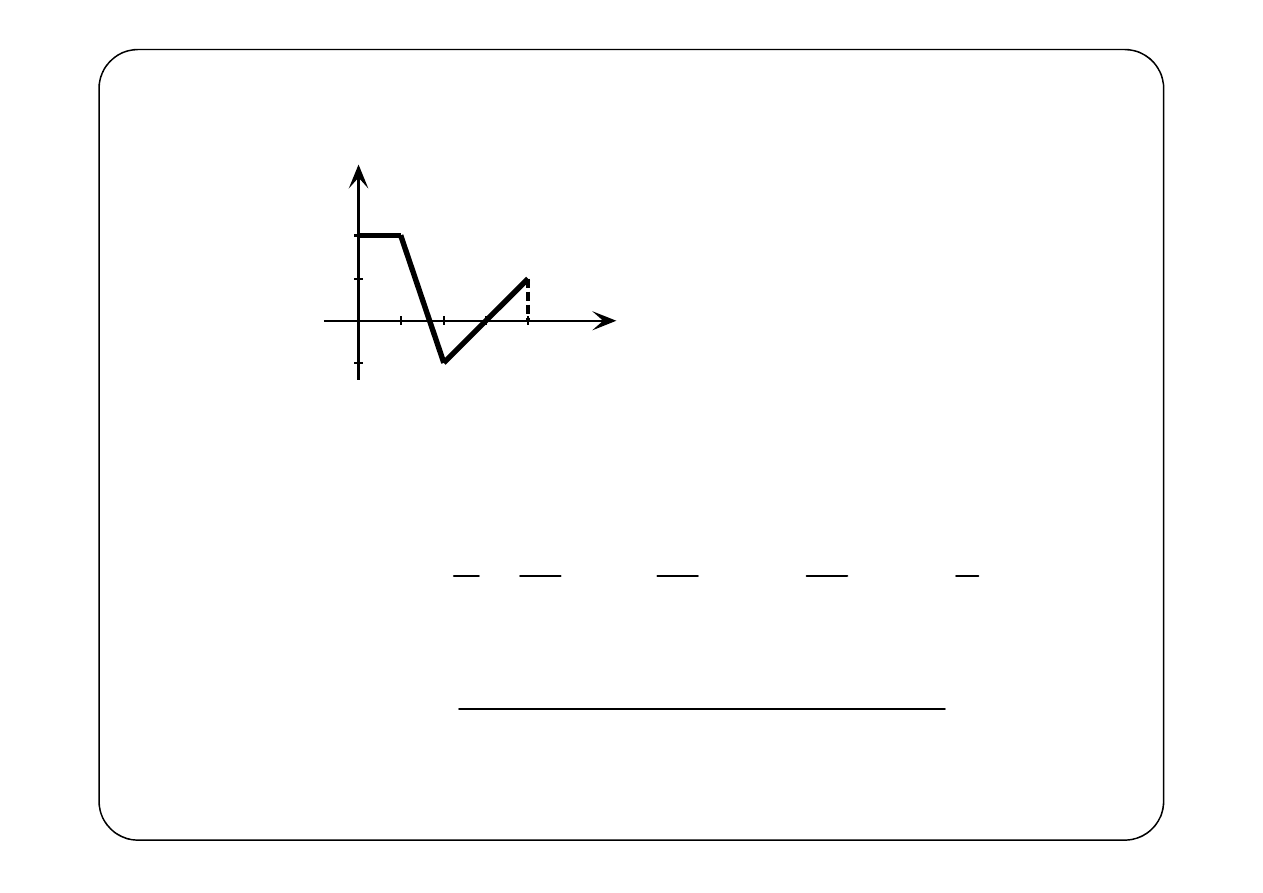
Przykład 5.
f(t)
t
1
2
1
2
3
4
–1
( )
( ) ( ) ( ) (
) (
) (
) (
) (
)
2
3
1
1
4
2
2
4
4
4
f t
t
t
t
t
t
t
t
t
= ⋅
−
−
− +
−
− − −
− −
−
1
1
1
1
1
( )
( ) ( ) ( ) (
) (
) (
) (
) (
)
2
3
1
1
4
2
2
4
4
4
f t
t
t
t
t
t
t
t
t
= ⋅
−
−
− +
−
− − −
− −
−
1
1
1
1
1
( )
( )
{ }
(
)
2
4
4
2
2
2
2
4
2
2
3
4
1
1
e
e
e
e
2
3e
4e
1
e
s
s
s
s
s
s
s
F s
f t
s
s
s
s
s
s
s
s
−
−
−
−
−
−
−
=
= −
+
−
−
=
−
+
− +
=
L
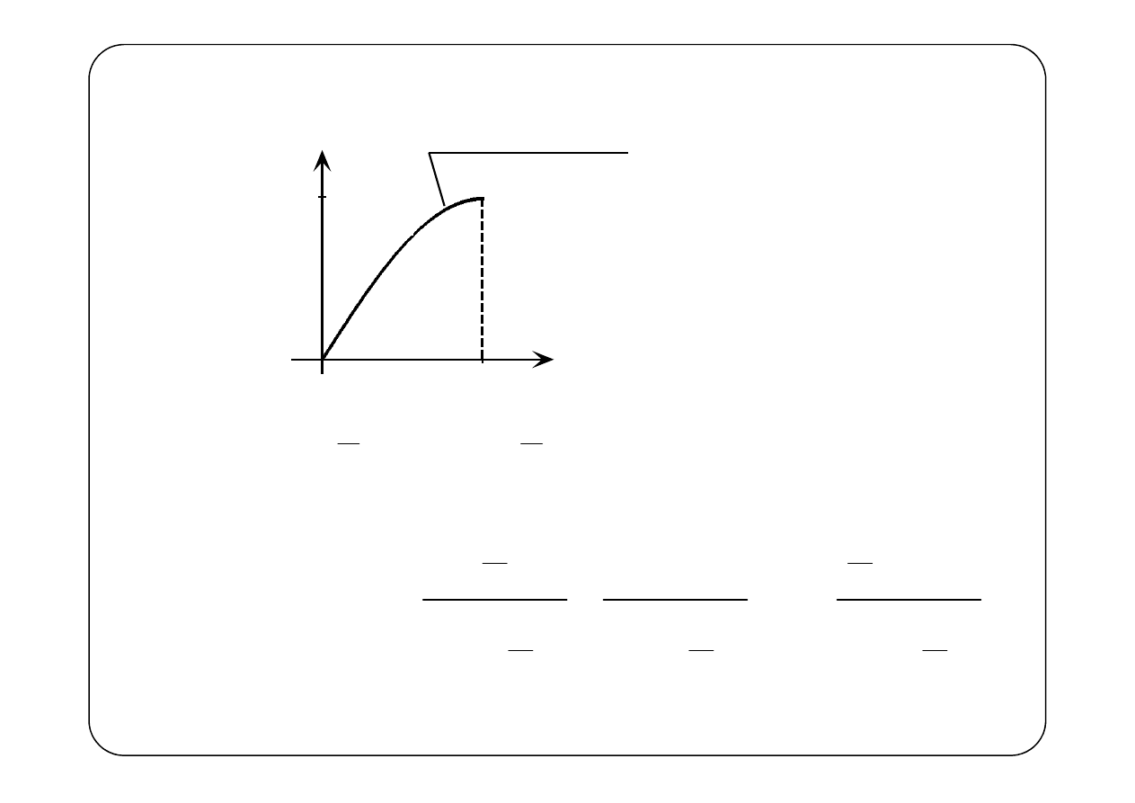
Przykład 6.
f(t)
t
1
1
"ćwiartka" sinusoidy
( )
( )
( ) ( )
π
π
sin
cos
1
1
2
2
f t
t
t
t
t
=
⋅
−
− ⋅
−
1
1
( )
( )
{ }
( )
( )
( )
2
2
2
2
2
2
π
π
e
2
2
e
π
π
π
2
2
2
s
s
s
s
F s
f t
s
s
s
−
−
−
=
=
−
=
+
+
+
L
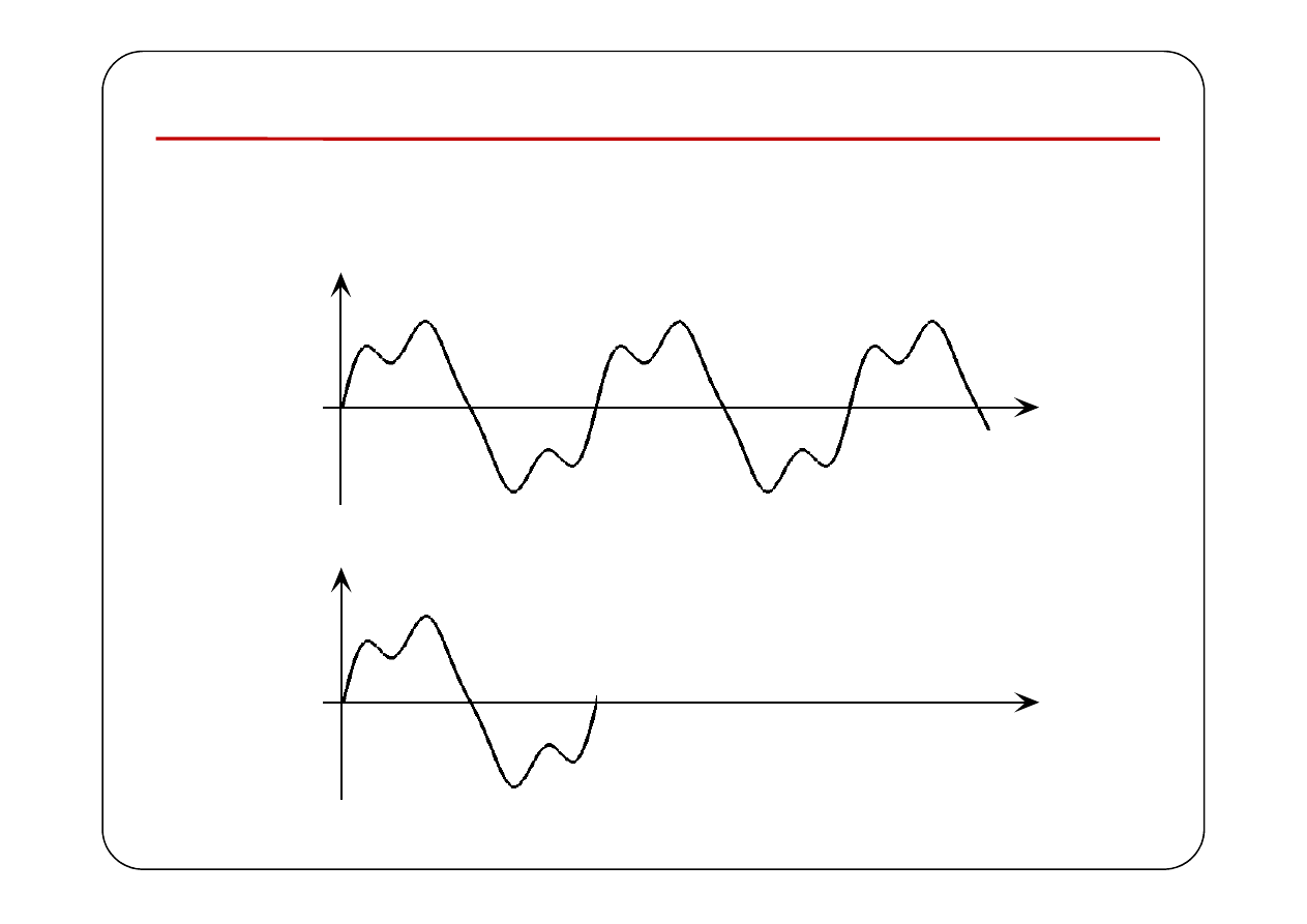
Transformata funkcji okresowej
( )
(
)
( )
,
1, 2,...,
0
dla
0
f t
f t
kT
k
f t
t
=
−
=
≡
<
f(t)
T
2T
t
T
f
T
(t)
t
T
f(t) – f
T
(t)
t
2T
( )
( )
(
) (
)
T
f t
f
t
f t
T
t
T
−
=
−
−
1
Niech
( )
{ }
( )
f t
F s
=
L
( )
{ }
( )
( )
{
}
( )
T
T
f t
F s
f
t
F
s
=
=
L
L
Wówczas
( )
( )
( )
e
sT
T
F s
F
s
F s
−
−
=
( )
( )
1 e
T
sT
F
s
F s
−
=
−
czyli
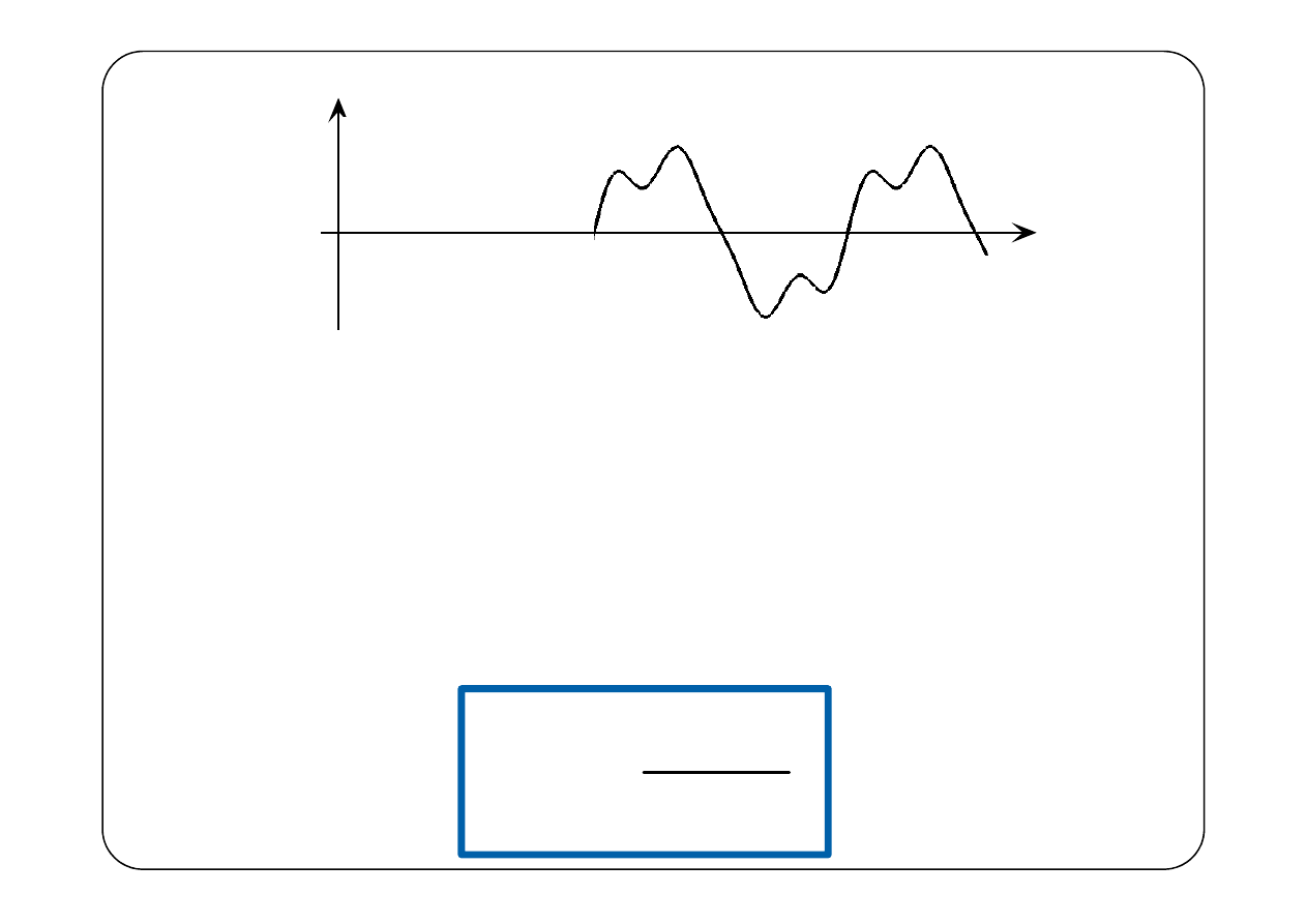
Przykład 7.
f(t)
t
1
1
3
2
T = 1
f
T
(t)
1
t
1
( )
( )
( ) ( )
sin π
sin π
1
1
T
f
t
t
t
t
t
=
⋅
+
− ⋅
−
1
1
( )
( )
{
}
(
)
2
2
π 1 e
π
s
T
T
F
s
f
t
s
−
+
=
=
+
L
( )
( )
{ }
( )
(
)
(
)(
)
2
2
π 1 e
1 e
π
1 e
s
T
s
s
F s
F s
f t
s
−
−
−
+
=
=
=
−
+
−
L
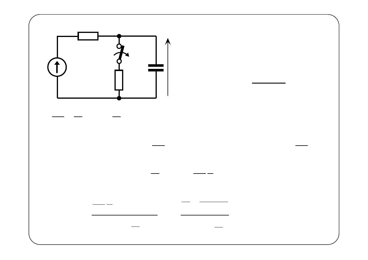
R
R
0
E
0
C
K
t = 0
u(t)
E
0
= const.
Warunek początkowy
( )
0
0
0
0
R
u
E
R
R
− = +
( )
0
d
1
1
,
0
d
u
C
u t
E
t
t
R
R
+
=
>
( )
{ }
( )
{ }
( ) ( )
{ }
0
0
d
,
0
,
d
E
u
u t
U s
sU s
u
E
t
s
=
=
−
−
=
L
L
L
( ) ( )
( )
0
1
1
0
E
C sU s
u
U s
R
R s
−
− +
=
( )
( )
( )
0
0
0
0
1
1
0
1
1
sCR
E
Cu
R
R
R
R s
U s
E
sC
s sC
R
R
+
+
−
+
=
=
+
+

( )
( )
{
}
1
?
u t
U s
−
=
=
L
( )
(
)
0
0
0
0
0
1
1
1
1
1
sCR
R
R
R
R
U s
E
E
s
R
R
s
s sC
RC
R
+ +
=
=
−
+
+
+
( )
( )
1
0
0
1
e
t
RC
R
u t
E
t
R
R
−
=
−
+
1

Obliczanie transformat odwrotnych
Niech
( )
( )
( )
( ) ( )
( )
( )
,
,
— wielomiany,
st
st
L s
F s
L s
M s
L s
M s
n
M s
=
<
=
Ponadto
( )
(
)
1
n
k
k
M s
s
s
=
=
−
∏
Czyli pierwiastki mianownika (bieguny
funkcji F(s)) są jednokrotne
Wówczas F(s) można rozłożyć na ułamki proste
Wówczas F(s) można rozłożyć na ułamki proste
( )
1
n
k
k
k
c
F s
s
s
=
=
−
∑
( )
( )
{
}
( )
1
1
e
k
n
s t
k
k
f t
F s
c
t
−
=
=
=
∑
1
L
gdzie
(
) ( )
k
k
k
s s
c
s
s
F s
=
= −
Transformata odwrotna

Przykład 1.
( ) ( )( )( )
2
3
23
14
1
4
1
s
s
F s
s
s
s
+
+
=
+
+
−
( )
3
1
2
1
4
1
c
c
c
F s
s
s
s
=
+
+
+
+
−
(
) ( )
(
)(
)
2
1
1
3
23
14
1
1
4
1
s
s
s
c
s
F s
s
s
=−
+
+
= +
=
=
+
−
1
2
4
1
4
1
s
s
s
−
=
+
+
+
+
−
(
)(
)
(
) ( )
(
)(
)
(
) ( )
(
)(
)
1
1
2
2
4
4
2
3
1
1
4
1
3
23
14
4
2
1
1
3
23
14
1
4
1
4
s
s
s
s
s
s
s
s
s
s
c
s
F s
s
s
s
s
c
s
F s
s
s
=−
=−
=−
=−
=
=
+
−
+
+
= +
=
= −
+
−
+
+
= −
=
=
+
+
( )
(
)
( )
4
e
2e
4e
t
t
t
f t
t
−
−
=
−
+
1

Przykład 2.
( ) ( )
(
)
2
2
4
11
2
4
2
10
s
s
F s
s
s
s
+
−
=
+
+
+
( )
1
0
1
2
4
2
10
k s
k
c
F s
s
s
s
+
=
+
+
+ +
(
) ( )
1
4
4
1
s
c
s
F s
=−
= +
=
1
1
k
=
−
= +
⇒
= −
0
0
0
1
0
1
1
0
1
1
0 :
3
3
20
4
10
3
1
1
1:
6
3
3
9
k
s
k
k
k
k
k
s
k
k
=
−
= +
⇒
= −
= −
− +
=
= −
− = +
⇒
− + = −
( )
(
)
(
)
2
2
2
1
3
3
1
1
3
3
2
4
4
2
10
1
9
1
9
s
s
F s
s
s
s
s
s
s
−
+
=
+
=
+
−
+
+
+ +
+
+
+
+
( )
(
) ( )
4
e
e
3cos3
2sin 3
t
t
f t
t
t
t
−
−
=
+
−
1

Niech
( )
( )
( )
( ) ( )
( )
( )
,
,
— wielomiany,
st
st
L s
F s
L s
M s
L s
M s
n
M s
=
<
=
( )
(
)
( )
1
1
,
st
k
m
m
k
k
k
k
M s
s
s
M s
n
α
α
=
=
=
−
= =
∑
∏
α
k
— krotność pierwiastka s
k
Rozkład na ułamki proste ma teraz postać
Rozkład na ułamki proste ma teraz postać
( )
(
)
1
1
k
m
kl
l
k
l
k
c
F s
s
s
α
=
=
=
−
∑∑
(
)
(
)
( )
1
d
! d
k
k
k
k
l
kl
k
l
k
s s
c
s
s
F s
l
s
α
α
α
α
−
−
=
=
−
−

Ponieważ
(
)
( )
( )
1
1
e
1 !
k
s t
l
kl
kl
l
k
c
c
t
t
l
s
s
−
−
=
−
−
1
L
( )
( )
{
}
( )
( )
1
1
e
k
k
m
s t
l
kl
c
f t
F s
t
t
α
−
−
=
=
=
∑∑
1
L
więc
( )
( )
{
}
( )
( )
( )
( )
1
1
1
1
1
1
1
e
1 !
e
1 !
k
k
k
s t
l
kl
k
l
m
s t
l
kl
k
l
f t
F s
t
t
l
c
t
t
l
α
−
−
=
=
−
=
=
=
=
=
−
=
−
∑∑
∑ ∑
1
1
L
Przykład 3.
( )
(
)(
)
3
1
2
1
s
F s
s
s
−
=
+
+
( )
(
) (
)
23
11
21
22
2
3
2
1
1
1
c
c
c
c
F s
s
s
s
s
=
+
+
+
+
+
+
+
(
) ( )
(
)
11
3
2
2
1
2
3
1
s
s
s
c
s
F s
s
=−
=−
−
= +
=
=
+
(
) ( )
(
)
(
) ( )
(
)
(
)
(
)
(
) ( )
(
)
(
)
2
3
23
1
1
3
22
2
2
1
1
1
2
3
21
2
2
3
1
1
1
1
1
2
2
2
1
d
3
1
3
d
2
2
1 d
1 d
3
3
1
3
2!
2 d
d
2
2
s
s
s
s
s
s
s
s
s
s
c
s
F s
s
s
s
c
s
F s
s
s
s
c
s
F s
s
s
s
s
=−
=−
=−
=−
=−
=−
=−
=−
=−
−
= +
=
= −
+
+ − −
=
+
=
=
=
+
+
−
=
+
=
=
= −
+
+

( )
(
) (
)
2
3
3
3
3
2
2
1
1
1
F s
s
s
s
s
=
−
+
−
+
+
+
+
( )
( )
{
}
(
)
( )
1
2
2
3e
3 3
e
t
t
f t
F s
t
t
t
−
−
−
=
=
+ − + −
1
L

Niech
( )
( )
( )
( ) ( )
( )
( )
,
,
— wielomiany,
st
st
L s
F s
L s
M s
L s
M s
n
M s
=
≥
=
( )
st L s
n
p
= +
Wówczas
( )
( )
( )
( )
( )
( )
( )
1
1
,
st
st
p
i
i
L s
L s
F s
k s
L s
M s
M s
M s
=
=
+
<
∑
( )
( )
( )
( )
( )
1
0
,
st
st
i
i
F s
k s
L s
M s
M s
M s
=
=
=
+
<
∑
( )
( )
δ
i
i
i
i
k s
k
t
≙
( )
( )
{
}
( )
( )
( )
( )
1
1
1
0
δ
p
i
i
i
L s
f t
F s
k
t
M s
−
−
=
=
=
+
∑
L
L

Przykład 4.
( )
3
2
2
6
14
11
4
4
s
s
s
F s
s
s
+
+
+
=
+
+
( )
(
)
(
)
(
)
2
2
2
2
3
2
4 1
2
1
2
2
2
2
2
2
2
s
s
F s
s
s
s
s
s
s
s
+
+ −
= + +
= + +
= + +
−
+
+
+
+
( )
( )
{
}
( )
( ) (
)
( )
1
2
δ
2
δ
2
e
t
f t
F s
t
t
t
t
−
−
′
=
=
+
+ −
1
L
Przykład 5.
Przykład 5.
( )
3
2
3
2
5
2
5
s
s
s
F s
s
s
s
+ + −
=
+
+
( )
(
)
(
)
(
)
2
2
2
2
2
4
5
2
5 2
1
2
1
1
1
2
5
2
5
1
4
s
s
s
s
s
F s
s
s s
s
s s
s
s
+ +
+ + +
= −
= −
= − −
+ +
+ +
+
+
( )
( )
{
}
( )
(
)
( )
1
δ
1 e sin 2
t
f t
F s
t
t
t
−
−
=
=
− +
1
L

Niech
( )
( )
( )
( )
( )
1
e
,
i
k
i
st
i
i
i
i
L s
F s
s
s
M
s
Φ
Φ
−
=
=
=
∑
Wówczas
( )
{
}
( ) ( )
( )
{
}
(
) (
)
1
1
,
e
i
i
st
s
t
t
s
t
t
t
t
Φ
ϕ
Φ
ϕ
−
−
−
=
=
−
−
1
1
L
L
( )
{
}
(
) (
)
1
e
i
st
i
i
i
i
s
t
t
t
t
Φ
ϕ
−
−
=
−
−
1
L
( )
( )
{
}
(
) (
)
1
1
k
i
i
i
i
f t
F s
t
t
t
t
ϕ
−
=
=
=
−
−
∑
1
L

Przykład 6.
( )
(
)
2
2
e
1
s
s
F s
s
s
−
−
=
+
( ) ( ) ( )
( )
( )
2
2
1
2
2
1
1
e
e
1
1
s
s
F s
s
s
s s
s
s
Φ
Φ
−
−
=
−
=
−
+
+
( ) ( )
( )
(
)
( )
1
1
1
1
1
1 e
,
1
1
t
s
t
t
s
s
s s
Φ
ϕ
−
=
= −
⇒
= −
+
+
1
( ) ( )
( )
(
)
( )
( )
(
)
( )
(
)
( )
1
1
1
2
2
2
2
2
1 e
,
1
1
0
1
1
1
1
1 e
,
1
1
2
t
s
t
t
s
s
s s
t
s
t
t
t
s
s
s
s
s
t
Φ
ϕ
Φ
ϕ
−
=
= −
⇒
= −
+
+
=
=
=
− +
⇒
= − +
+
+
=
1
1
( )
( )
{
}
(
)
( )
( )
(
)
2
1
1 e
3 e
2
t
t
f t
F s
t
t
t
− −
−
−
=
= −
− − +
−
1
1
L

Niech
( )
( )
1 e
sT
s
F s
Ψ
−
=
−
Jeżeli
to F(s) jest transformatą
funkcji okresowej f(t), która w przedziale 0
≤
t < T jest równa
( )
{
}
1
0
dla
s
t
T
Ψ
−
≡
>
L
( )
( )
{
}
1
.
T
f
t
s
Ψ
−
=
L
Jeżeli to F(s)
( )
{
}
1
0, czyli nie znika dla
s
t
T
Ψ
−
≠
>
L
Jeżeli to F(s)
nie jest transformatą funkcji okresowej. Wówczas
( )
{
}
0, czyli nie znika dla
s
t
T
Ψ
≠
>
L
( )
( )
(
)
2
3
1 e
e
e
sT
sT
sT
F s
s
Ψ
−
−
−
=
+
+
+
+
⋯
( )
( )
{
}
( ) ( )
(
) (
)
(
) (
)
1
2
2
f t
F s
t
t
t
T
t
T
t
T
t
T
ψ
ψ
ψ
−
=
=
=
+
−
−
+
−
−
+
1
1
1
⋯
L
( )
( )
{
}
1
t
s
ψ
Ψ
−
=
L
gdzie
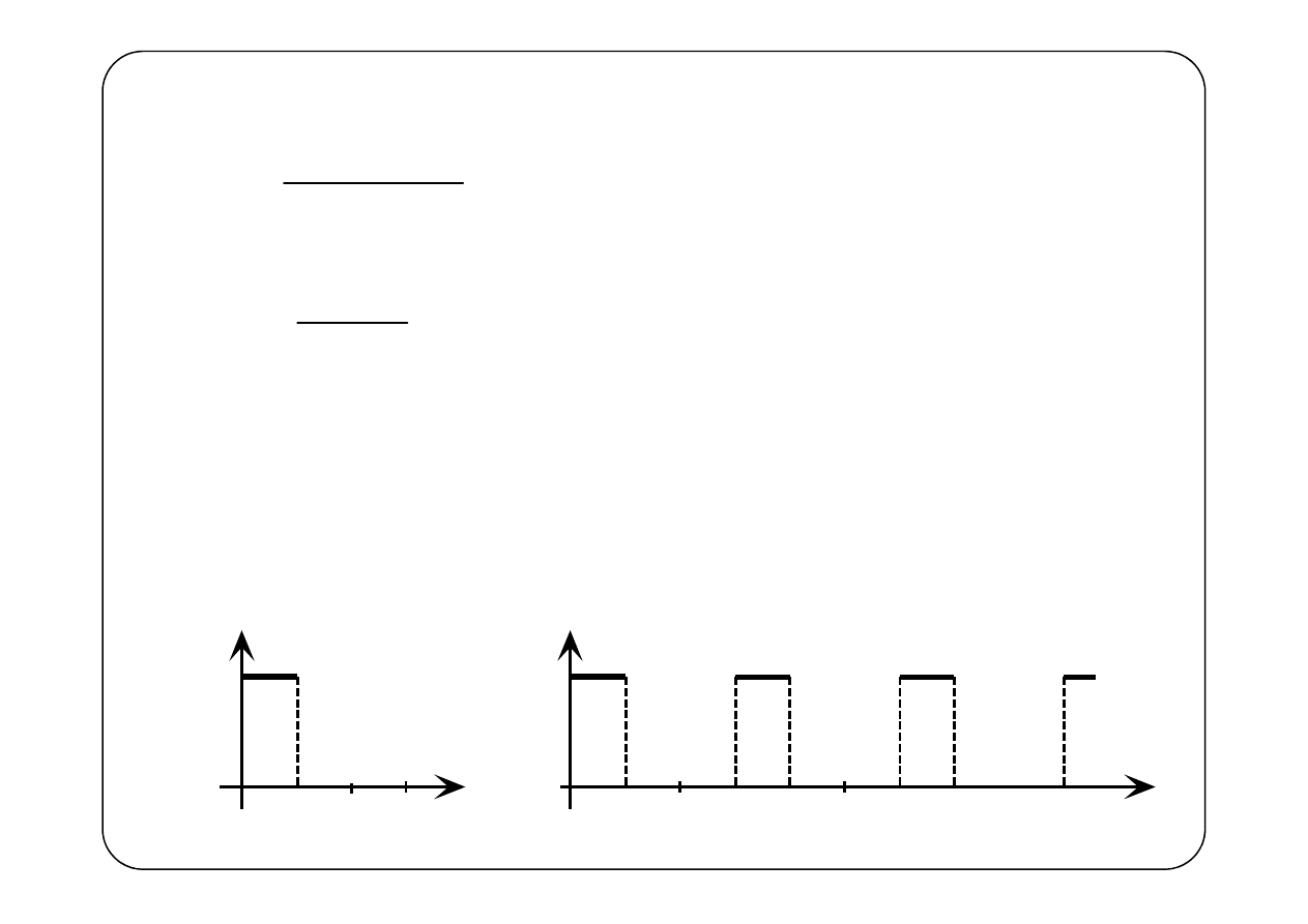
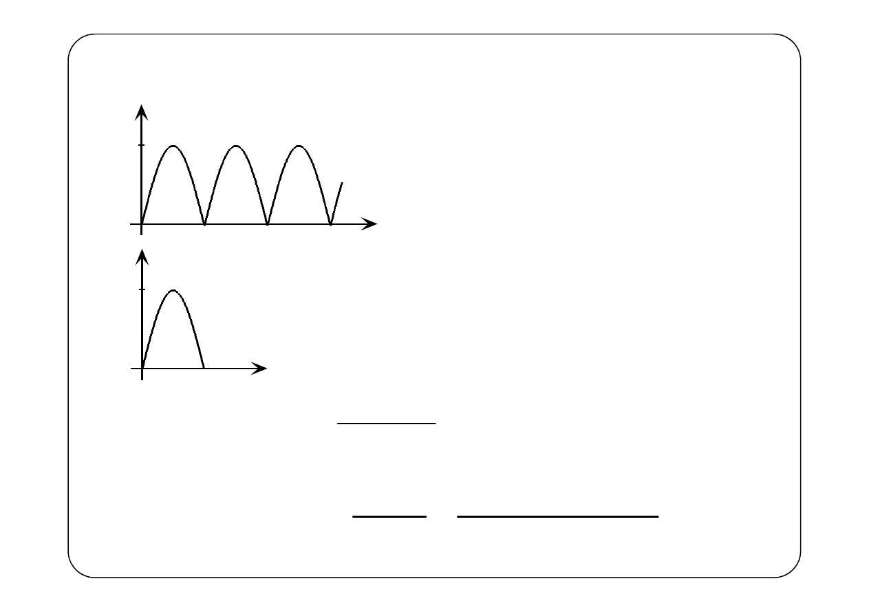
Przykład 7.
( )
(
)
3
1 e
1 e
s
s
F s
s
−
−
−
=
−
( )
( )
{
}
( ) ( )
1
1 e
,
1
s
s
s
t
t
s
Ψ
Ψ
−
−
−
=
=
−
−
1
1
L
Ponieważ więc
( )
{
}
1
0
dla
3,
s
t
T
Ψ
−
≡
> =
L
( )
{
}
( )
1
T
s
f
t
Ψ
−
=
L
( )
( )
{
}
1
f t
F s
−
=
L
i jest funkcją okresową o okresie T = 3.
t
1
2
3
1
2
3
4
5
6
t
( )
( )
{
}
1
T
f
t
s
Ψ
−
=
L
( )
( )
{
}
1
f t
F s
−
=
L
1
1
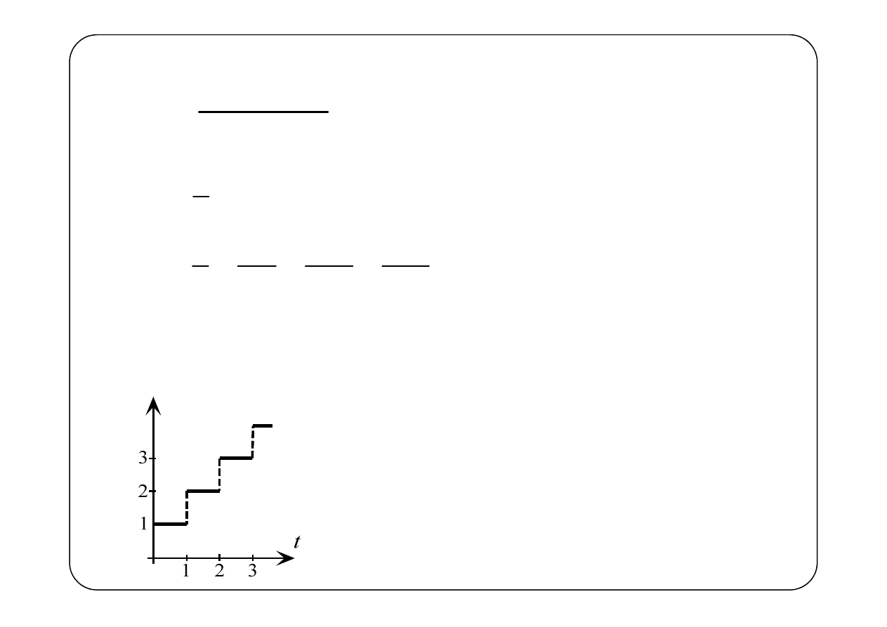
Przykład 8.
( )
(
)
1
1 e
s
F s
s
−
=
−
( )
( )
{
}
( )
1
1
,
s
s
t
s
Ψ
Ψ
−
=
=
1
L
( )
( )
( )
{
}
( ) ( ) (
) (
)
2
3
1
1
e
e
e
1
2
3
s
s
s
F s
s
s
s
s
f t
F s
t
t
t
t
−
−
−
−
= +
+
+
+
=
=
+
− +
− +
− +
1
1
1
1
⋯
⋯
L
( )
( )
{
}
( ) ( ) (
) (
)
1
1
2
3
f t
F s
t
t
t
t
−
=
=
+
− +
− +
− +
1
1
1
1
⋯
L
( )
( )
{
}
1
f t
F s
−
=
L
Wyszukiwarka
Podobne podstrony:
Przekształcenia Laplacea cz1
Przekształcenie Laplace
Przekształcenie Laplace'a
4 Przeksztalcenie Laplacea
Przekszta?nie Laplace 1
Przekształcenie Laplace-tabela
03 przeksztalcenie laplace
Przekształcenie Laplace'a
4 Przeksztalcenie Laplacea CW
02 Przeksztalcenie Laplace, MiBM Politechnika Poznanska, IV semestr, automatyka, egzamin, pierdoly,
Rozwiazywanie rownan rozniczkowych Przeksztalcenia Laplacea, Nauka i Technika, Automatyka, Teoria st
Przekształcenia Laplace'a, Matematyka
Przekształcenie Laplace
02 Przeksztalecenie Laplace
4 Przeksztalcenie Laplacea
więcej podobnych podstron