http://www.mece.ualberta.ca/tutorials/ansys/PP/DataPlotting/Pri

Using Tables to Post Process Results

Introduction

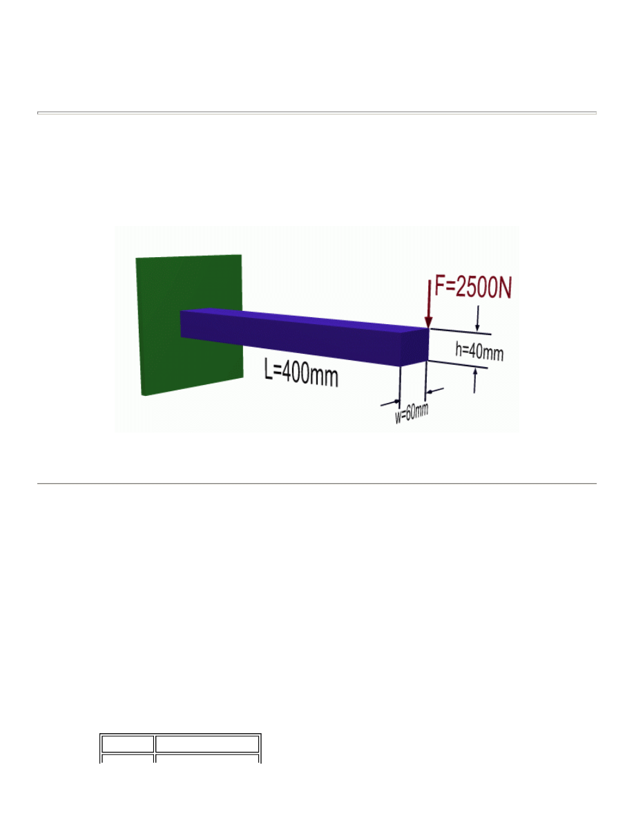
This tutorial was created using ANSYS 7.0 The purpose of this tutorial is to outline the steps required to plot

Vertical Deflection vs. Length of the following beam using tables, a special type of array. By plotting this data
on a curve, rather than using a contour plot, finer resolution can be achieved.

This tutorial will use a steel beam 400 mm long, with a 40 mm X 60 mm cross section as shown above. It will
be rigidly constrained at one end and a -2500 N load will be applied to the other.

Preprocessing: Defining the Problem

1. Give the example a Title

Utility Menu > File > Change Title ...

/title, Use of Tables for Data Plots

2. Open preprocessor menu

ANSYS Main Menu > Preprocessor

/PREP7

3. Define Keypoints

Preprocessor > Modeling > Create > Keypoints > In Active CS...

K,#,x,y,z

We are going to define 2 keypoints for this beam as given in the following table:

Keypoint Coordinates (x,y,z)

University of Alberta ANSYS Tutorials - www.mece.ualberta.ca/tutorials/ansys/AT/AdvancedX-SecResults/...

4. Create Lines

Preprocessor > Modeling > Create > Lines > Lines > In Active Coord

L,1,2

Create a line joining Keypoints 1 and 2

5. Define the Type of Element

Preprocessor > Element Type > Add/Edit/Delete...

For this problem we will use the BEAM3 (Beam 2D elastic) element. This element has 3 degrees of
freedom (translation along the X and Y axes, and rotation about the Z axis).

6. Define Real Constants

Preprocessor > Real Constants... > Add...

In the 'Real Constants for BEAM3' window, enter the following geometric properties:

i. Cross-sectional area AREA: 2400

ii. Area moment of inertia IZZ: 320e3

iii. Total beam height: 40

This defines a beam with a height of 40 mm and a width of 60 mm.

7. Define Element Material Properties

Preprocessor > Material Props > Material Models > Structural > Linear > Elastic > Isotropic

In the window that appears, enter the following geometric properties for steel:

i. Young's modulus EX: 200000

ii. Poisson's Ratio PRXY: 0.3

8. Define Mesh Size

Preprocessor > Meshing > Size Cntrls > ManualSize > Lines > All Lines...

For this example we will use an element edge length of 20mm.

9. Mesh the frame

Preprocessor > Meshing > Mesh > Lines > click 'Pick All'

Solution Phase: Assigning Loads and Solving

1. Define Analysis Type

Solution > Analysis Type > New Analysis > Static

ANTYPE,0

(0,0)

(400,0)

University of Alberta ANSYS Tutorials - www.mece.ualberta.ca/tutorials/ansys/AT/AdvancedX-SecResults/...

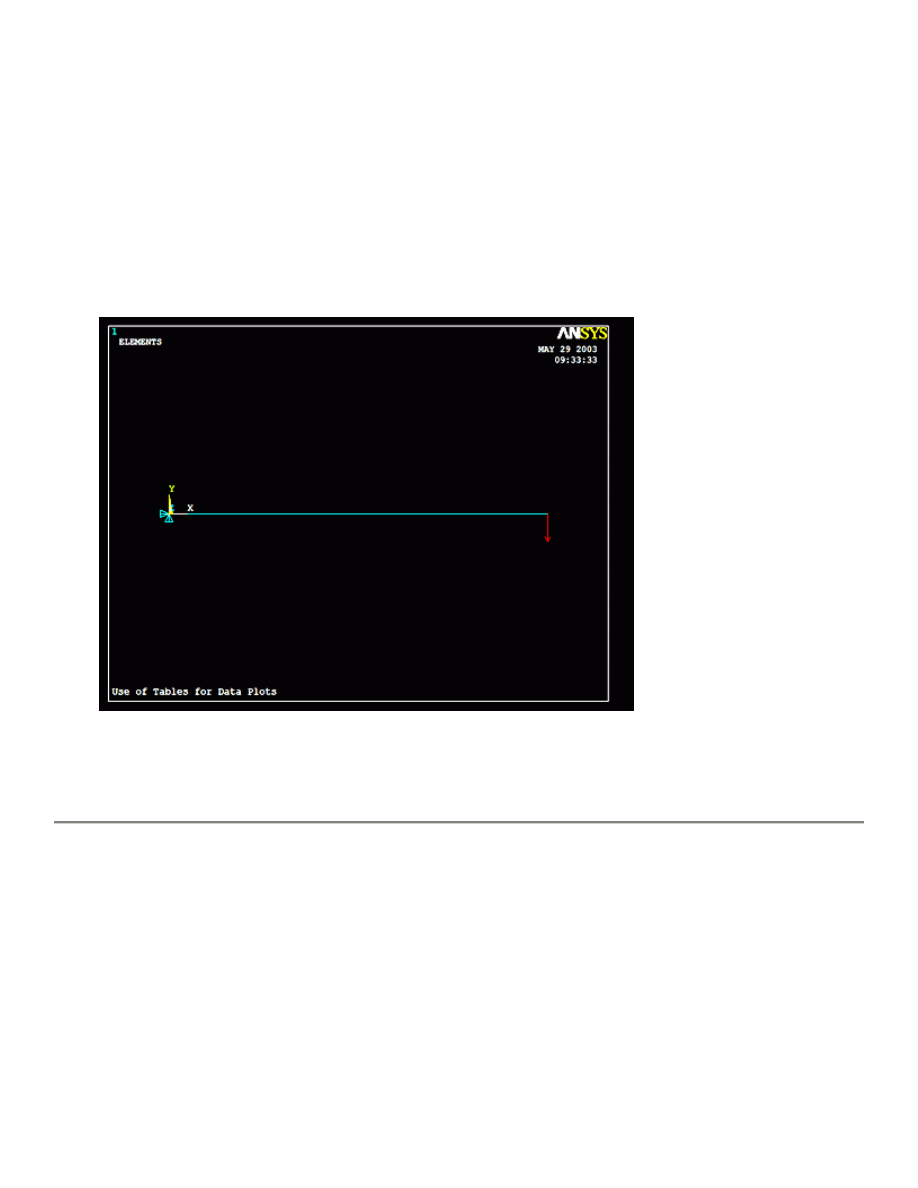
2. Apply Constraints

Solution > Define Loads > Apply > Structural > Displacement > On Keypoints

Fix keypoint 1 (ie all DOF constrained)

3. Apply Loads

Solution > Define Loads > Apply > Structural > Force/Moment > On Keypoints
Apply a load of -2500N on keypoint 2.

The model should now look like the figure below.

4. Solve the System

Solution > Solve > Current LS

SOLVE

Postprocessing: Viewing the Results

It is at this point the tables come into play. Tables, a special type of array, are basically matrices that can be
used to store and process data from the analysis that was just run. This example is a simplified use of tables, but

they can be used for much more. For more information type

help

in the command line and search for 'Array

Parameters'.

1. Number of Nodes

Since we wish to plot the verticle deflection vs length of the beam, the location and verticle deflection of

each node must be recorded in the table. Therefore, it is necessary to determine how many nodes exist in

University of Alberta ANSYS Tutorials - www.mece.ualberta.ca/tutorials/ansys/AT/AdvancedX-SecResults/...

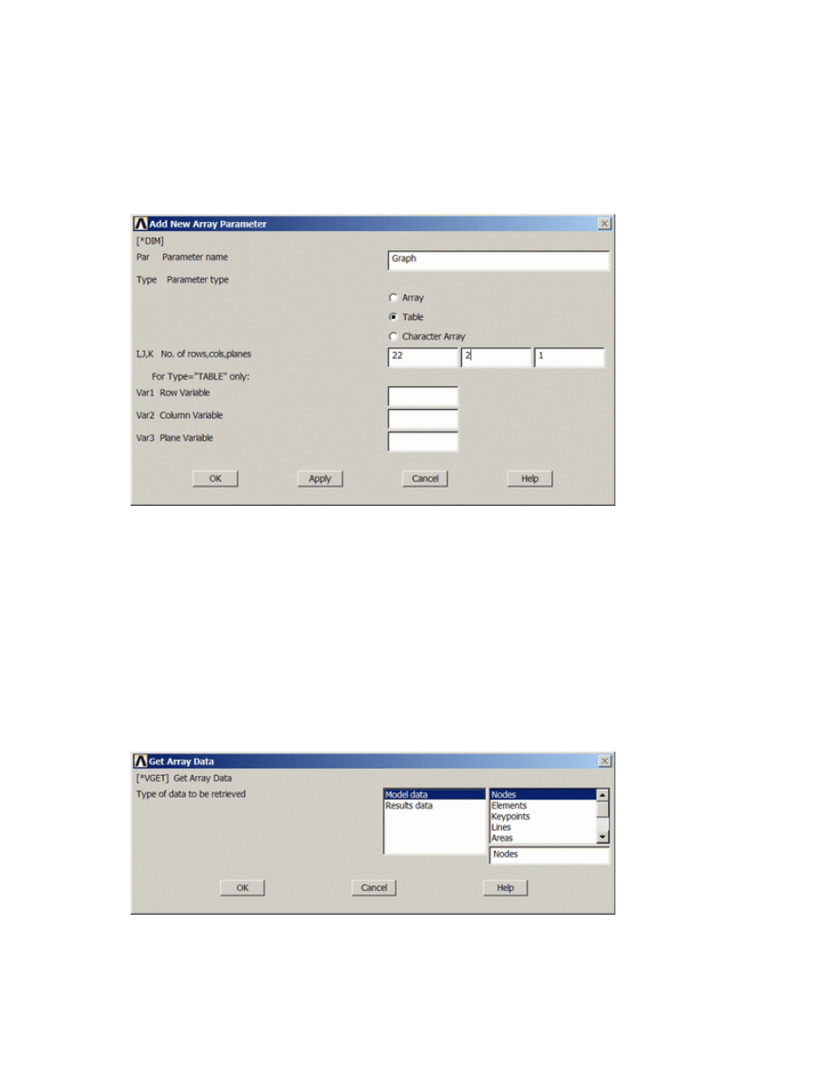
the model. Utility Menu > List > Nodes... > OK. For this example there are 21 nodes. Thus the table

must have at least 21 rows.

2. Create the Table

{

Utility Menu > Parameters > Array Parameters > Define/Edit > Add

{

The window seen above will pop up. Fill it out as shown [Graph > Table > 22,2,1]. Note there are

22 rows, one more than the number of nodes. The reason for this will be explained below. Click
OK and then close the 'Define/Edit' window.

3. Enter Data into Table

First, the horizontal location of the nodes will be recorded

{

Utility Menu > Parameters > Get Array Data ...

{

In the window shown below, select Model Data > Nodes

{

Fill the next window in as shown below and click OK [Graph(1,1) > All > Location > X]. Naming
the array parameter 'Graph(1,1)' fills in the table starting in row 1, column 1, and continues down
the column.

University of Alberta ANSYS Tutorials - www.mece.ualberta.ca/tutorials/ansys/AT/AdvancedX-SecResults/...

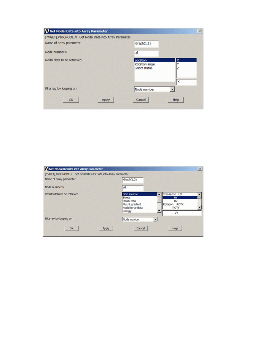
Next, the vertical displacement will be recorded.

{

Utility Menu > Parameters > Get Array Data ... > Results data > Nodal results

{

Fill the next window in as shown below and click OK [Graph(1,2) > All > DOF solution > UY].

Naming the array parameter 'Graph(1,2)' fills in the table starting in row 1, column 2, and continues
down the column.

4. Arrange the Data for Ploting

Users familiar with the way ANSYS numbers nodes will realize that node 1 will be on the far left, as it is
keypoint 1, node 2 will be on the far right (keypoint 2), and the rest of the nodes are numbered

sequentially from left to right. Thus, the second row in the table contains the data for the last node. This
causes problems during plotting, thus the information for the last node must be moved to the final row of

the table. This is why a table with 22 rows was created, to provide room to move this data.

{

Utility Menu > Parameters > Array Parameters > Define/Edit > Edit

University of Alberta ANSYS Tutorials - www.mece.ualberta.ca/tutorials/ansys/AT/AdvancedX-SecResults/...

{

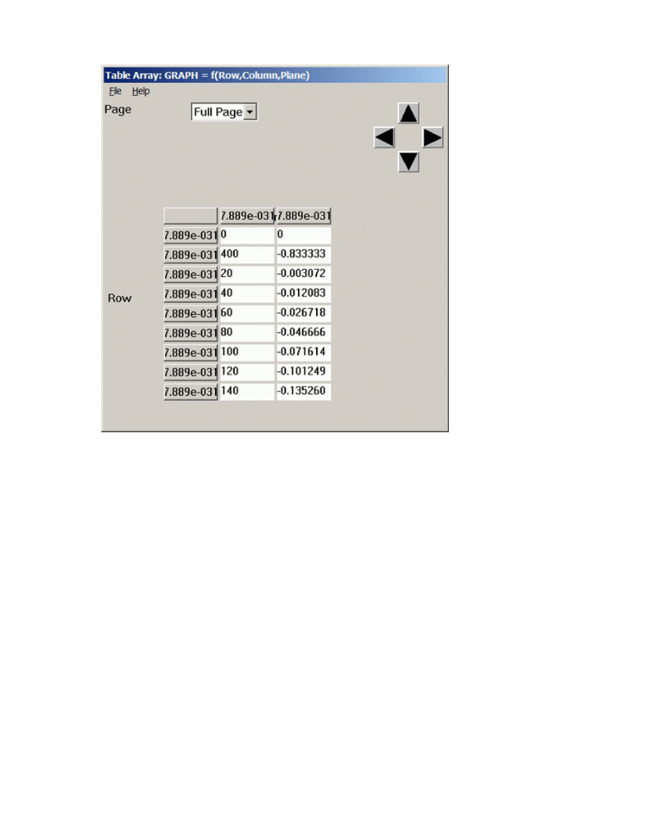
The data for the end of the beam (X-location = 400, UY = -0.833) is in row two. Cut one of the

cells to be moved (right click > Copy or Ctrl+X), press the down arrow to get to the bottom of the
table, and paste it into the appropriate column (right click > Paste or Ctrl+V). When both values

have been moved check to ensure the two entries in row 2 are zero. Select File > Apply/Quit

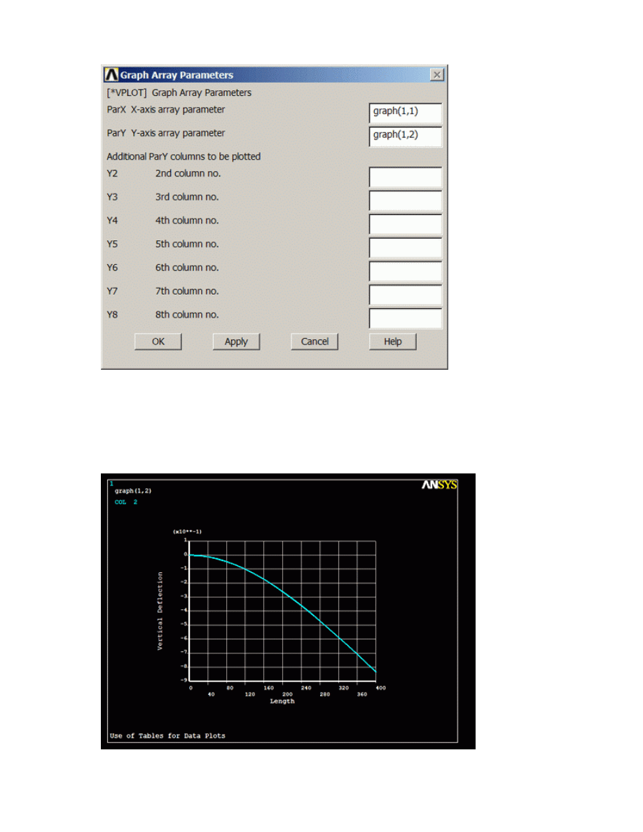
5. Plot the Data

{

Utility Menu > Plot > Array Parameters

{

The following window will pop up. Fill it in as shown, with the X-location data on the X-axis and

the vertical deflection on the Y-axis.

University of Alberta ANSYS Tutorials - www.mece.ualberta.ca/tutorials/ansys/AT/AdvancedX-SecResults/...

{

To change the axis labels select Utility Menu > Plot Ctrls > Style > Graphs > Modify Axes ...

{

To see the changes to the labels, select Utility Menu > Replot

{

The plot should look like the one seen below.

University of Alberta ANSYS Tutorials - www.mece.ualberta.ca/tutorials/ansys/AT/AdvancedX-SecResults/...

Command File Mode of Solution

The above example was solved using a mixture of the Graphical User Interface (or GUI) and the command
language interface of ANSYS. This problem has also been solved using the

ANSYS command language

interface

that you may want to browse. Open the file and save it to your computer. Now go to 'File > Read

input from...' and select the file.

University of Alberta ANSYS Tutorials - www.mece.ualberta.ca/tutorials/ansys/AT/AdvancedX-SecResults/...