Copyright

© by SIAM. Unauthorized reproduction of this article is prohibited.

SIAM J. M

ATRIX

A

NAL.

A

PPL

.

c

2008 Society for Industrial and Applied Mathematics

Vol. 30, No. 4, pp. 1320–1338

OPTIMAL SCALING OF GENERALIZED AND POLYNOMIAL

EIGENVALUE PROBLEMS

∗

T. BETCKE

†

Abstract. Scaling is a commonly used technique for standard eigenvalue problems to improve

the sensitivity of the eigenvalues. In this paper we investigate scaling for generalized and polynomial
eigenvalue problems (PEPs) of arbitrary degree. It is shown that an optimal diagonal scaling of a
PEP with respect to an eigenvalue can be described by the ratio of its normwise and componentwise
condition number. Furthermore, the effect of linearization on optimally scaled polynomials is investi-
gated. We introduce a generalization of the diagonal scaling by Lemonnier and Van Dooren to PEPs
that is especially effective if some information about the magnitude of the wanted eigenvalues is
available and also discuss variable transformations of the type λ = αμ for PEPs of arbitrary degree.

Key words. polynomial eigenvalue problem, balancing, scaling, condition number, backward

error

AMS subject classifications. 65F15, 15A18

DOI. 10.1137/070704769

1. Introduction. Scaling of standard eigenvalue problems Ax = λx is a well-

established technique that is implemented in the LAPACK routine xGEBAL. It goes
back to work by Osborne [14] and Parlett and Reinsch [15]. The idea is to find a
diagonal matrix D that scales the rows and columns of A ∈ C

n×n

in a given norm

such that

D

−1

ADe

i

= e

∗

i

D

−1

AD,

i = 1, . . . , n,

where e

i

is the ith unit vector. This is known as balancing. LAPACK uses the 1-

norm. Balancing matrix rows and columns can often reduce the effect of rounding
errors on the computed eigenvalues. However, as Watkins demonstrated [19], there
are also cases in which balancing can lead to a catastrophic increase of the errors in
the computed eigenvalues.

For generalized eigenvalue problems (GEPs) Ax = λBx, a scaling technique pro-

posed by Ward [18] is implemented in the LAPACK routine xGGBAL. Its aim is to
find diagonal matrices D

1

and D

2

such that the elements of D

1

AD

2

and D

1

BD

2

are

scaled as equal in magnitude as possible.

A different approach for the scaling of GEPs is proposed by Lemonnier and Van

Dooren [11]. In section 5 we will come back to this. It is interesting to note that
the default behavior of LAPACK (and also of MATLAB) is to scale nonsymmetric
standard eigenvalue problems but not to scale GEPs.

In this paper we discuss the scaling of polynomial eigenvalue problems (PEPs) of

the form

(1.1)

P (λ)x := (λ

A

+

· · · + λA

1

+ A

0

)x = 0,

A

k

∈ C

n×n

, A

= 0, ≥ 1.

Every λ ∈ C for which there exists a solution x ∈ C

n

\{0} of P (λ)x = 0 is called an

∗

Received by the editors October 8, 2007; accepted for publication (in revised form) by L. De Lath-

auwer April 30, 2008; published electronically October 16, 2008. This work was supported by Engi-
neering and Physical Sciences Research Council grant EP/D079403/1.

http://www.siam.org/journals/simax/30-4/70476.html

†

School of Mathematics, The University of Manchester, Oxford Road, Manchester, M13 9PL, UK

([e-mail], http://www.ma.man.ac.uk/˜tbetcke).

1320

Copyright

© by SIAM. Unauthorized reproduction of this article is prohibited.

SCALING OF EIGENVALUE PROBLEMS

1321

eigenvalue of P with associated right eigenvector x. We will also need left eigenvectors
y ∈ C

n

\{0} defined by y

∗

P (λ) = 0.

In section 2 we review the definition of condition numbers and backward errors

for the PEP (1.1). Then in section 3 we investigate diagonal scalings of (1.1) of the
form D

1

P (λ)D

2

, where D

1

and D

2

are diagonal matrices in the set

D

n

:=

{D : D ∈ C

n×n

is diagonal and det(D) = 0}.

We show that the minimal achievable normwise condition number of an eigenvalue by
diagonal scaling of P (λ) can be bounded by its componentwise condition number. This
gives easily computable conditions on whether the condition number of eigenvalues
can be improved by scaling. The results of that section can be applied to generalized
linear and higher degree polynomial problems.

The most widely used technique to solve PEPs of degree ≥ 2 is to convert

the associated matrix polynomial into a linear pencil, the process of linearization,
and then solve the corresponding GEP. In section 4 we investigate the difference
between scaling before or after linearizing the matrix polynomial. Then in section 5 we
introduce a heuristic scaling strategy for PEPs that generalizes the idea of Lemonnier
and Van Dooren. It is applicable to arbitrary polynomials of degree ≥ 1 and includes
a weighting factor that, given some information about the magnitude of the wanted
eigenvalues, can crucially improve the normwise condition numbers of eigenvalues
after scaling.

Fan, Lin and Van Dooren [3] propose a transformation of variables of the form

λ = αμ for some parameter α for quadratic polynomials whose aim is to improve the
backward stability of numerical methods for quadratic eigenvalue problems (QEPs)
that are based on linearization. In section 6 we extend this variable transformation
to matrix polynomials of arbitrary degree ≥ 2.

Numerical examples illustrating our scaling algorithms are presented in section 7.

We conclude with practical remarks on how to put the results of this paper into
practice.

Scaling routines for standard and generalized eigenvalue problems often include

a preprocessing step that attempts to remove isolated eigenvalues by permutation of
the matrices. This is, for example, implemented in the LAPACK routines xGBAL and
xGGBAL. Since the permutation algorithm described in [18] can be easily adapted for
matrix polynomials, we will not discuss this further in this paper. But nevertheless,
it is advisable to use this preprocessing step also for PEPs to reduce the problem
dimension if possible.

All notation is standard. For a matrix A, we denote by |A| the matrix of absolute

values of the entries of A. Similarly, |x| for a vector x denotes the absolute values of
the entries of x. The vector of all ones is denoted by e; that is, e =

1, 1, . . . , 1

T

∈ R

n

.

2. Normwise and componentwise error bounds. An important tool to mea-

sure the quality of an approximate eigenpair (˜

x, ˜

λ) of the PEP P (λ)x = 0 is its

normwise backward error. With ΔP (λ) =

k=0

λ

k

ΔA

k

it is defined for the 2-norm

by

η

P

˜

x, ˜

λ

:= min

:

P

˜

λ

+ ΔP

˜

λ

˜

x = 0, ΔA

k

2

≤ A

k

2

, k = 0 :

.

Tisseur [17] shows that

η

P

˜

x, ˜

λ

=

r

2

˜

α˜

x

2

,

Copyright

© by SIAM. Unauthorized reproduction of this article is prohibited.

1322

TIMO BETCKE

where r = P (˜

λ)˜

x and ˜

α =

k=0

|˜λ|

k

A

k

2

. The normwise backward error η(˜

λ) of a

computed eigenvalue ˜

λ is defined as

η

P

˜

λ

= min

x∈C

n

x=0

η

P

x, ˜

λ

.

It follows immediately [17, Lemma 3] that η

P

(˜

λ) = (˜

αP (˜

λ)

−1

2

)

−1

.

The sensitivity of an eigenvalue is measured by the condition number. It relates

the forward error, that is, the error in the computed eigenvalue ˜

λ, and the backward

error η

P

(˜

λ). To first order (meaning up to higher terms in the backward error) one

has

(2.1)

forward error

≤ backward error × condition number.

The condition number of a simple, finite, nonzero eigenvalue λ = 0 is defined by

κ

P

(λ) := lim

→0

sup

|Δλ|

|λ|

:

P (λ + Δλ) + ΔP (λ + Δλ)

(x + Δx) = 0,

ΔA

k

2

≤ A

k

2

, k = 0 :

.

Let x be a right eigenvector and y be a left eigenvector associated with the eigenvalue
λ of P . Then κ

P

(λ) is given by [17, Theorem 5]

(2.2)

κ

P

(λ) =

y

2

x

2

α

|y

∗

P

(λ)x||λ|

,

α =

k=0

|λ|

k

A

k

2

.

Backward error and condition number can also be defined in a componentwise

sense. The componentwise backward error of an eigenpair (˜

x, ˜

λ) is

(2.3) ω

P

˜

x, ˜

λ

:= min

:

P

˜

λ

+ ΔP

˜

λ

˜

x = 0; |ΔA

k

| ≤ |A

k

|, k = 0 :

.

The componentwise condition number of a simple, finite, nonzero eigenvalue λ is
defined as

cond

P

(λ) := lim

→0

sup

|Δλ|

|λ|

:

P (λ + Δλ) + ΔP (λ + Δλ)

(x + Δx) = 0,

|ΔA

k

| ≤ |A

k

|, k = 0 :

.

(2.4)

The following theorem gives explicit expressions for these quantitites.

Theorem 2.1.

The componentwise backward error of an approximate eigenpair

(˜

x, ˜

λ) is given by

(2.5)

ω

P

(˜

x, ˜

λ) = max

i

|r

i

|

A|˜

x|

i

,

A :=

k=0

|˜λ|

k

|A

k

|,

Copyright

© by SIAM. Unauthorized reproduction of this article is prohibited.

SCALING OF EIGENVALUE PROBLEMS

1323

where r

i

denotes the ith component of the vector P (˜

λ)˜

x. The componentwise condi-

tion number of a simple, finite, nonzero eigenvalue λ with associated left and right
eigenvectors y and x is given by

(2.6)

cond

P

(λ) =

|y|

∗

A|x|

|λ||y

∗

P

(λ)x|

,

A :=

k=0

|λ|

k

|A

k

|.

Proof. The proof is a slight modification of the proofs of [5, Theorems 3.1 and

3.2] along the lines of the proof of [17, Theorem 1].

Surveys of componentwise error analysis are contained in [8, 9]. The compo-

nentwise backward error and componentwise condition number are invariant under
multiplication of P (λ) from the left and the right with nonsingular diagonal matri-
ces. In the next section we will use this property to characterize optimally scaled
eigenvalue problems.

3. Optimal scalings. In this section we introduce the notion of an optimal

scaling with respect to a certain eigenvalue and give characterizations of it.

Ultimately, we are interested in computing eigenvalues to as many digits as pos-

sible. Hence, we would like to find a scaling that leads to small forward errors. If
we assume that we use a backward stable algorithm, that is, the backward error is
only a small multiple of the machine precision, then it follows from (2.1) that we can
hope to compute an eigenvalue to many digits of accuracy by finding a scaling that
minimizes the condition number.

In the following we define what we mean by a scaling of a matrix polynomial

P (λ).

Definition 3.1.

Let P (λ) ∈ C

n×n

be a matrix polynomial. A scaling of P (λ) is

the matrix polynomial D

1

P (λ)D

2

, where D

1

, D

2

∈ D

n

.

It is immediately clear that the eigenvalues of a matrix polynomial P (λ) are

invariant under scaling. Furthermore, if (y, x, λ) is an eigentriplet of P (λ) with eigen-
value λ and left and right eigenvector y and x, respectively, then an eigentriplet of
the scaling D

1

P (λ)D

2

is (D

−∗

1

y, D

−1

2

x, λ).

The following definition defines an optimal scaling of P (λ) with respect to a given

eigenvalue λ in terms of minimizing the condition number of λ.

Definition 3.2.

Let λ be a simple, finite, nonzero eigenvalue of the matrix

polynomial P (λ). We call P (λ) optimally scaled with respect to λ if

κ

P

(λ) =

inf

D

1

,D

2

∈D

n

κ

D

1

P D

2

(λ).

This definition of optimal scaling depends on the eigenvalue λ. We cannot expect

that an optimal scaling for one eigenvalue also gives an optimal scaling for another
eigenvalue. The following theorem states that a PEP is almost optimally scaled with
respect to an eigenvalue λ, if the componentwise and normwise condition numbers
of λ are close to each other. Furthermore, it gives explicit expressions for scaling
matrices D

1

, D

2

∈ D

n

that achieve an almost optimal scaling.

Theorem 3.3.

Let λ be a simple, finite, nonzero eigenvalue of an n × n matrix

polynomial P (λ) with associated left and right eigenvectors y and x, respectively. Then

(3.1)

1

√

n

cond

P

(λ) ≤

inf

D

1

,D

2

∈D

n

κ

D

1

P D

2

(λ) ≤ n cond

P

(λ).

Moreover, if all the entries of y and x are nonzero, then for

D

1

= diag(

|y|), D

2

= diag(

|x|),

Copyright

© by SIAM. Unauthorized reproduction of this article is prohibited.

1324

TIMO BETCKE

we have

(3.2)

κ

D

1

P D

2

(λ) ≤ n cond

P

(λ).

Proof.

Let A :=

k=0

|λ|

k

|A

k

| and α :=

k=0

|λ|

k

A

k

2

.

Using

|B|

2

≤

√

nB

2

[9, Lemma 6.6] for any matrix B ∈ C

n×n

, the lower bound follows from

cond

P

(λ) =

|y|

∗

A|x|

|λ||y

∗

P

(λ)x|

≤

y

2

x

2

A

2

|λ||y

∗

P

(λ)x|

≤

√

nαy

2

x

2

|λ||y

∗

P

(λ)x|

=

√

nκ

P

(λ),

and the fact that the componentwise condition number is invariant under diagonal
scaling. For > 0 define the vectors ˜

y and ˜

x by

˜

y

i

=

y

i

, y

i

= 0

,

y

i

= 0

˜

x

i

=

x

i

, x

i

= 0

,

x

i

= 0

and consider the diagonal matrices

D

1

= diag(

|˜y|), D

2

= diag(

|˜x|).

Using

B

2

≤ e

∗

|B|e for any matrix B ∈ C

n×n

[9, Table 6.2], we have

κ

D

1

P D

2

(λ) =

D

−1

1

y

2

D

−1

2

x

2

k=0

|λ|

k

D

1

A

k

D

2

2

|λ||y

∗

P

(λ)x|

≤

n

k=0

|λ|

k

e

∗

|D

1

A

k

D

2

|e

|λ||y

∗

P

(λ)x|

=

n

k=0

|λ|

k

· |˜y|

∗

· |A

k

| · |˜x|

|λ||y

∗

P

(λ)x|

−→ n cond

P

(λ) as → 0.

(3.3)

The upper bounds in (3.1) and (3.2) follow immediately.

Theorem 3.3 is restricted to finite and nonzero eigenvalues. Assume that λ = 0

is an eigenvalue. Then we have to replace relative componentwise and normwise
condition numbers by the absolute condition numbers

κ

(a)

P

(λ) =

y

2

x

2

α

|y

∗

P

(λ)x|

,

cond

(a)

P

(λ) =

|y|

∗

A|x|

|y

∗

P

(λ)x|

.

With these condition numbers Theorem 3.3 is also valid for zero eigenvalues. If P (λ)
has an infinite eigenvalue, the reversal rev P (λ) := λ

P (1/λ) has a zero eigenvalue,

and we can apply Theorem 3.3 using absolute condition numbers to rev P (λ).

While Theorem 3.3 applies to generalized linear and polynomial problems, it

does not immediately apply to standard problems of the form Ax = λx. The crucial
difference is that for standard eigenvalue problems we assume the right-hand side
identity matrix to be fixed and only allow scalings of the form D

−1

AD that leave the

identity unchanged. However, if λ is an eigenvalue of A with associated left and right
eigenvectors y and x that have nonzero entries, we can still define D

1

= diag(

|y|) and

D

2

= diag(

|x|) to obtain the generalized eigenvalue problem

(3.4)

D

1

AD

2

v = λD

1

D

2

v,

where x = D

2

v. Since D

1

D

2

has positive diagonal entries there exists ˆ

D such that

ˆ

D

2

= D

1

D

2

. We then obtain from (3.4) the standard eigenvalue problem

(3.5)

ˆ

D

−1

D

1

AD

2

ˆ

D

−1

˜

x = λ˜

x,

Copyright

© by SIAM. Unauthorized reproduction of this article is prohibited.

SCALING OF EIGENVALUE PROBLEMS

1325

where ˜

x = ˆ

DD

−1

2

x and |˜

x| =

|y

1

||x

1

|, . . . ,

|y

n

||x

n

|

T

. For the scaled left eigen-

vector ˜

y we have ˜

y = ˆ

DD

−1

1

y and |˜

y| = |˜

x|. If we define the normwise condition

number k

A

(λ) and the componentwise condition number c

A

(λ) for the eigenvalue λ

of a standard eigenvalue problem by

1

k

A

(λ) =

y

2

x

2

|λ||y

T

x|

,

c

A

(λ) =

|y|

T

|x|

|λ||y

T

x|

,

it follows for the scaling D

−1

AD, where D = D

2

ˆ

D

−1

= D

−1

1

ˆ

D that

c

A

(λ) = k

D

−1

AD

(λ).

But this scaling is not always useful as

D

−1

AD

2

can become large if x or y contain

tiny entries.

There is a special case in which the scaling (3.5) also minimizes

D

−1

AD

2

. If λ

is the Perron root of an irreducible and nonnegative matrix A, the corresponding left
and right eigenvectors y and x can be chosen to have positive entries. After scaling
by D as described above, we have k

D

−1

AD

(λ) = 1 and D

−1

AD

2

= λ. This was

investigated by Chen and Demmel in [2] who proposed a weighted balancing which is
identical to the scaling described above for nonnegative and irreducible A.

Theorem 3.3 gives us an easy way to check whether a matrix polynomial P is

nearly optimally scaled with respect to an eigenvalue λ. We only need to compute
the ratio

(3.6)

κ

P

(λ)

cond

P

(λ)

=

y

2

x

2

k=0

|λ|

k

A

k

2

|y|

∗

k=0

|λ|

k

|A

k

|

|x|

after computing the eigenvalues and eigenvectors. If an eigensolver already returns
normwise condition numbers, this is only a little extra effort. If

κ

P

(λ)

cond

P

(λ)

n the

eigensolver can give a warning to the user that the problem is badly scaled and
that the error in the computed eigenvalue λ is likely to become smaller by rescaling
P . Furthermore, from Theorem 3.3 it follows that a polynomial is nearly optimally
scaled if the entries of the left and right eigenvectors have equal magnitude. This
motivates a heuristic scaling algorithm, which is discussed in section 5.

At the end we would like to emphasize that a diagonal scaling which improves

the condition numbers of the eigenvalues needs not necessarily be a good scaling for
eigenvectors. An example is the generalized linear eigenvalue problem L(λ)x = 0,
where

L(λ) = λ

⎡
⎣

1

0

0

0

2

0

0

0

2

⎤
⎦ +

⎡
⎣

0

1 + 2

· 10

−8

2

2

10

−8

1

1

1 + 10

−8

−1

⎤
⎦ .

One eigenvalue is λ = 1 with associated right eigenvector x =

1

−1 10

−8

T

and

left eigenvector y =

1
3

1
3

−1

T

. The condition number

2

of the eigenvector x before

scaling is approximately 33.1. After scaling with D

1

= diag(

|y|) and D

2

= diag(

|x|),

it increases to 1.70 · 10

9

. For the corresponding eigenvalue λ = 1 we have κ

L

(1)

≈ 21.8

and after scaling κ

D

1

LD

2

(1)

≈ 19.6. However, in most of our experiments we could

not observe an increase of the eigenvector condition number after scaling.

1

Choose E = I, F = 0, and B = I in Theorems 2.5 and 3.2 of [5].

2

The condition number of the eigenvector was computed using Theorem 2.7 from [5] with the

normalization vector g =

1

0

0

T

.

Copyright

© by SIAM. Unauthorized reproduction of this article is prohibited.

1326

TIMO BETCKE

4. Scalings and linearizations. The standard way to solve the PEP (1.1) of

degree ≥ 2 is to convert P (λ) into a linear pencil

L(λ) = λX + Y

having the same spectrum as P (λ) and then solve the eigenproblem for L. Formally,
L(λ) is a linearization if

E(λ)L(λ)F (λ) =

P (λ)

0

0

I

(−1)n

for some unimodular E(λ) and F (λ) [4, section 7.2]. For example,

(4.1)

C

1

(λ) = λ

⎡
⎢

⎢

⎢

⎢

⎣

A

0

· · ·

0

0

I

n

. .. ...

..

.

. .

.

. .

.

0

0

· · ·

0

I

n

⎤
⎥

⎥

⎥

⎥

⎦

+

⎡
⎢

⎢

⎢

⎣

A

−1

A

−2

· · ·

A

0

−I

n

0

· · ·

0

..

.

. ..

. ..

..

.

0

· · ·

−I

n

0

⎤
⎥

⎥

⎥

⎦

is a linearization of P (λ), called the first companion form. In [12] Mackey, Mackey,
Mehl, and Mehrmann identified two vector spaces of pencils that are potential lin-
earizations of P (λ). Let Λ := [λ

−1

, λ

−2

, . . . , 1]

T

. Then these spaces are defined

by

L

1

(P ) =

L(λ) : L(λ)(Λ ⊗ I

n

) = v ⊗ P (λ), v ∈ C

,

L

2

(P ) =

L(λ) : (Λ

T

⊗ I

n

)L(λ) = ˜

v

T

⊗ P (λ), ˜v ∈ C

.

The first companion linearization belongs to

L

1

(P ) with v = e

1

. Furthermore, the

pencils in

L

1

(P ) and L

2

(P ) that are not linearizations form a closed nowhere dense

subset of measure zero in these spaces [12, Theorem 4.7].

Another important space of potential linearizations is given by

DL(P ) := L

1

(P ) ∩ L

2

(P ).

In [12, Theorem 5.3] it is shown that each pencil L(λ) ∈ DL(P ) is uniquely defined
by a vector v ∈ C

such that

L(λ)(Λ ⊗ I

n

) = v ⊗ P (λ),

Λ

T

⊗ I

n

L(λ) = v

T

⊗ P (λ).

There is a well-defined relationship between the eigenvectors of linearizations L(λ) ∈

DL(P ) and eigenvectors of P (λ); namely, for finite eigenvalues λ x is a right eigenvec-
tor of P (λ) if and only if Λ ⊗ x is a right eigenvector of L(λ) and y is a left eigenvector
of P (λ) if and only if Λ ⊗ y is a left eigenvector of L(λ) [12, Theorems 3.8 and 3.14].

A simple observation is that scaling P (λ) leads to a scaling of L(λ) within the

same space of potential linearizations.

Lemma 4.1.

Let L(λ) ∈ S(P ) with vector v, where S(P ) = L

1

(P ), L

2

(P ), or

DL(P ). Then (I

n

⊗ D

1

)L(λ)(I

n

⊗ D

2

) is in

S(D

1

P D

2

) with the same vector v, where

D

1

, D

2

∈ C

n×n

are nonsingular matrices.

Proof. The statements follow immediately from the identities

(I ⊗ D

1

)L(λ)(I ⊗ D

2

)(Λ

⊗ I

n

) = v ⊗ D

1

P (λ)D

2

Copyright

© by SIAM. Unauthorized reproduction of this article is prohibited.

SCALING OF EIGENVALUE PROBLEMS

1327

and

Λ

T

⊗ I

n

(I ⊗ D

1

)L(λ)(I ⊗ D

2

) = ˜

v

T

⊗ D

1

P (λ)D

2

for matrices D

1

, D

2

∈ C

n×n

.

Hence, if we solve a PEP by a linearization in

L

1

(P ), L

2

(P ), or DL(P ), scaling of

the original polynomial P (λ) with matrices D

1

and D

2

is just a special scaling of the

linearization L(λ) with scaling matrices (I ⊗ D

1

) and (I ⊗ D

2

). If preserving structure

of the linearization is not an issue, we can scale the linearization L(λ) directly with
diagonal scaling matrices

D

1

and

D

2

that have 2n free parameters compared to the

2n free parameters in D

1

and D

2

. The following theorem gives a worst case bound

on the ratio between the optimal condition numbers with the two different scaling
strategies (i.e., scaling and then linearizing or linearizing and then scaling).

Theorem 4.2.

Let λ be a simple finite eigenvalue of P and let L(λ) ∈ DL(P )

with vector v. Then

inf

D

1

,D

2

∈D

n

κ

L

(λ; v; D

1

P D

2

)

≤

⎧

⎪

⎨
⎪

⎩

1/2

n

3/2

|λ|

2

−1

|λ|

2

−1

inf

˜

D

1

, ˜

D

2

∈D

n

κ

˜

D

1

L ˜

D

2

(λ) for |λ| ≥ 1,

1/2

n

3/2

|λ|

2(−1)

|λ|

2

−1

|λ|

2

−1

inf

˜

D

1

, ˜

D

2

∈D

n

κ

˜

D

1

L ˜

D

2

(λ)

for

|λ| < 1,

where κ

L

(λ; v; D

1

P D

2

) is the condition number of λ for the linearization

L(λ) ∈

DL(D

1

P D

2

) with vector v.

Proof. Let y and x be left and right eigenvectors of P (λ) associated with the

eigenvalue λ. Since L(λ) = λX +Y ∈ DL(P ), its left and right eigenvectors associated
with λ are Λ ⊗ y and Λ ⊗ x. Assume that y and x have no zero entries. The case
of zero entries follows by a limit process similar to that in the proof of Theorem 3.3.
Define D

1

= diag(

|y|) and D

2

= diag(

|x|). Since Λ ⊗ (D

−1

1

y)

2

=

Λ

2

D

−1

1

y

2

and

Λ ⊗ (D

−1

2

x)

2

=

Λ

2

D

−1

2

x

2

, we have

κ

L

(λ; v; D

1

P D

2

)

=

Λ

2

2

D

−1

1

y

2

D

−1

2

x

2

(

|λ|(I ⊗ D

1

)X(I ⊗ D

2

)

2

+

(I ⊗ D

1

)Y (I ⊗ D

2

)

2

)

|λ||

Λ

⊗ y

∗

X(Λ ⊗ x)|

,

and therefore by using

B

2

≤ e

∗

|B|e for any B ∈ C

n×n

κ

L

(λ; v; D

1

P D

2

)

≤

Λ

2

2

nˆ

e

∗

(

|λ||(I ⊗ D

1

)X(I ⊗ D

2

)

| + |(I ⊗ D

1

)Y (I ⊗ D

2

)

|)ˆe

|λ||

Λ

⊗ y

∗

X(Λ ⊗ x)|

for ˆ

e =

1

. . .

1

T

∈ R

n

. Assume that

|λ| ≥ 1. Since componentwise ˆe ≤ |Λ|⊗e =

|Λ| ⊗ e and

|Λ| ⊗ e

∗

(I ⊗ D

1

) =

|Λ ⊗ y|

∗

,

(I ⊗ D

2

)(

|Λ| ⊗ e) = |Λ ⊗ x|,

we obtain

(4.2)

κ

L

(λ; v; D

1

P D

2

)

≤ n

Λ

2

2

|Λ ⊗ y|

∗

(

|λ||X| + |Y |)|Λ ⊗ x|

|λ||

Λ

⊗ y

∗

X(Λ ⊗ x)|

= nΛ

2

2

cond

L

(λ).

It holds that

(4.3)

Λ

2

2

=

|λ|

2

− 1

|λ|

2

− 1

.

Copyright

© by SIAM. Unauthorized reproduction of this article is prohibited.

1328

TIMO BETCKE

Furthermore, from Theorem 3.3 we know that

(4.4)

1

√

n

cond

L

(λ) ≤

inf

˜

D

1

, ˜

D

2

∈D

n

κ

˜

D

1

L ˜

D

2

(λ).

Combining (4.2), (4.3), and (4.4), the proof for the case

|λ| ≥ 1 follows. The proof

for

|λ| < 1 is similar. The only essential difference is that now componentwise ˆe ≤

|Λ|

|λ|

−1

⊗ e.

Theorem 4.2 suggests that for eigenvalues that are large or small in magnitude

first linearizing and then scaling can in the worst case be significantly better than first
scaling and then linearizing. However, if we first linearize and then scale, the special
structure of the linearization is lost.

How sharp are these bounds?

In the following we discuss the case

|λ| ≥ 1.

For the case

|λ| < 1 analogous arguments can be used. Consider the QEP Q(λ) =

λ

2

A + λB + C, where

(4.5)

A =

−0.6 −0.1

2

0.1

,

B =

1

−0.1

0.6 −0.8

,

C =

3

· 10

7

7

· 10

7

−1 · 10

8

1.6 · 10

8

,

and its linearization in

DL(Q)

L(λ) = λX + Y := λ

A

0

0

−C

+

B

C

C

0

,

which corresponds to the vector v =

1

0

T

. One eigenvalue of this pencil is λ ≈

4.105·10

4

. If we first scale Q using the left and right eigenvectors associated with λ and

then linearize, this eigenvalue has the condition number 1.2 · 10

9

for the linearization.

If we first linearize the QEP and then scale the pencil L(λ) using the left and right
eigenvectors of λ for the linearization, this eigenvalue has the condition number 5.2.
The ratio between the condition numbers is in magnitude what we would expect from
applying Theorem 4.2.

However, Theorem 4.2 can be a large overestimate. Assume that P (λ) is already

almost optimally scaled in the sense of Theorem 3.3, that is,

|y| = |x| = e for the left

and right eigenvectors y and x associated with the simple finite eigenvalue λ of P .
Let L(λ) = λX + Y be a linearization of P and let D

1

and D

2

be scaling matrices

for L such that |D

−∗

1

˜

y| = |D

−1

2

˜

x| = e for the left and right eigenvectors ˜

y and ˜

x of L

associated with the eigenvalue λ. The ratio of the condition numbers of the eigenvalue
λ for the two pencils L and D

1

LD

2

is given by

(4.6)

κ

L

(λ)

κ

D

1

LD

2

(λ)

=

˜x

2

˜y

2

D

−∗

1

˜

y

2

D

−1

2

˜

x

2

|λ|X

2

+

Y

2

|λ|D

1

XD

2

2

+

D

1

Y D

2

2

.

If L(λ) ∈ DL(P ) (4.6) simplifies to

κ

L

(λ)

κ

D

1

LD

2

(λ)

=

1

|λ|

2

− 1

|λ|

2

− 1

|λ|X

2

+

Y

2

|λ|D

1

XD

2

2

+

D

1

Y D

2

2

since

|˜x| = |˜y| = |Λ ⊗ e|. This shows that for |λ| > 1 the upper bound in Theorem 4.2

can be attained only if

(4.7)

|λ|X

2

+

Y

2

|λ|D

1

XD

2

2

+

D

1

Y D

2

2

=: τ (λ)

Copyright

© by SIAM. Unauthorized reproduction of this article is prohibited.

SCALING OF EIGENVALUE PROBLEMS

1329

10

0

10

2

10

4

10

6

10

8

10

−14

10

−12

10

−10

10

−8

10

−6

10

−4

10

−2

10

0

A,B,C random

A, B, C as in (4.5)

λ

τ(λ)

Fig. 4.1

. The function τ (λ) for a large range of values in the case of a random 2

× 2 QEP and

the QEP from (4.5).

is approximately constant in the range of the eigenvalues in which we are interested.
For L(λ) ∈ DL(P ) the matrices D

1

and D

2

are given as

D

1

= D

2

=

⎡
⎢

⎣

|λ|

−1

I

. ..

I

⎤
⎥

⎦ = diag(|Λ|) ⊗ I.

It follows that for

|λ| large enough

(4.8)

τ (λ) ∼ γ|λ|

2−2

for some constant γ > 0 and therefore

κ

L

(λ)

κ

D

1

LD

2

(λ)

∼

γ

in that case.

In particular, if the upper left n × n block of X is in norm comparable or larger

than the other n×n subblocks of X, we expect a good agreement of the asymptotic in
(4.8) for all

|λ| > 1, where γ is not much larger than 1. Only if the n × n subblocks of

X and Y are of widely varying norm it is possible that τ (λ) is approximately constant
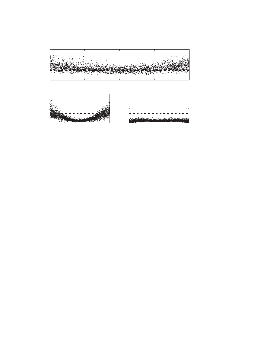
for a large range of values of λ, leading to the worst case bound in (4.2) being attained.

The situation is demonstrated in Figure 4.1. For a random 2

×2 QEP τ(λ) decays

like γ|λ|

−2

, where γ ≈ 1. For the QEP from (4.5) the function τ (λ) is almost constant

for a long time, leading to the worst case bound of Theorem 4.2 being attained in
these range of values. Then at about 10

4

it starts decaying like γ|λ|

−2

, where this

time γ is in the order of 10

8

.

One of the most frequently used linearizations for unstructured problems is the

companion form (4.1). Unfortunately, we cannot immediately apply the previous
results to it since the companion form is not in

DL(P ) but only in L

1

(P ). However,

we can still compare the ratio in (4.6). Consider the QEP Q(λ) = λ

2

A + λB + C.

Copyright

© by SIAM. Unauthorized reproduction of this article is prohibited.

1330

TIMO BETCKE

The companion linearization takes the form

C

1

(λ) = λ

A

I

+

B

C

−I 0

.

We assume that for the left and right eigenvectors y and x associated with the eigen-
value λ of Q we have |y| = |x| = e. Furthermore, let D

1

and D

2

again be chosen

such that

|D

−∗

1

˜

y| = |D

−1

2

˜

x| = e, where ˜

y and ˜

x are the corresponding left and right

eigenvectors for the eigenvalue λ of the companion linearization C

1

(λ) = λX + Y .

The relationship between the eigenvectors of C

1

and the eigenvectors of P associated

with a finite nonzero eigenvalue λ is given by

˜

x = Λ ⊗ x,

˜

y =

y

−

1

λ

C

∗

y

.

The formula for the left eigenvector is a consequence of [6, Theorem 3.2]. It follows
that

κ

C

1

(λ)

κ

˜

D

1

C

1

˜

D

2

(λ)

=

1

2n

1/2

|λ|

4

− 1

|λ|

2

− 1

1/2

n +

1

|λ|

2

C

∗

y

2

2

1/2

τ (λ).

If

|λ| 1 this simplifies to

κ

C

1

(λ)

κ

˜

D

1

C

1

˜

D

2

(λ)

≈

1

2

|λ|τ(λ),

which differs by a factor of

|λ| from the corresponding case using a DL(P ) linearization.

Asymptotically, we have

τ (λ) ∼ γ|λ|

−1

,

|λ| 1

for some factor γ and therefore

κ

C1

(λ)

κ

˜

D1C1 ˜

D2

(λ)

∼

γ

2

, where again we expect this asymptotic

to hold approximately for all

|λ| > 1 with a value of γ that is not much larger than 1

if the n × n subblocks of X and Y do not differ too widely in norm.

5. A heuristic scaling strategy. For standard eigenvalue problems the motiva-

tion of scaling algorithms is based on the observation that in floating point arithmetic
computed eigenvalues of a matrix A can be expected to be at least perturbed by an
amount of the order of

mach

A. Hence, by reducing A one hopes to reduce the

inaccuracies in the computed eigenvalues.

One way of minimizing

A is to find a nonsingular diagonal matrix D such that

the rows and columns of A are balanced in the sense that

(5.1)

D

−1

ADe

i

= e

∗

i

D

−1

AD,

i = 1, . . . , n.

Osborne [14] shows that if A is irreducible and · is the 2-norm in (5.1), then for
this D it holds that

!!

D

−1

AD

!!

F

= inf

ˆ

D∈D

n

!!

! ˆ

D

−1

A ˆ

D

!!

!

F

.

A routine that attempts to find a matrix D that balances the row and column norms of
A is built into LAPACK under the name xGEBAL. It uses the 1-norm in the balancing
condition (5.1). A description of the underlying algorithm is contained in [15].

Copyright

© by SIAM. Unauthorized reproduction of this article is prohibited.

SCALING OF EIGENVALUE PROBLEMS

1331

For generalized eigenvalue problems Ax = λBx, Ward [18] proposes to find non-

singular diagonal scaling matrices D

1

and D

2

such that the elements of the scaled

matrices D

1

AD

2

and D

1

BD

2

would have absolute values close to unity. Then the

relative perturbations in the matrix elements caused by computational errors would
be of similar magnitude. To achieve this Ward proposes to minimize the function

n

i,j=1

(r

i

+ c

j

+ log

|A

ij

|)

2

+ (r

i

+ c

j

+ log

|B

ij

|)

2

,

where the r

i

and c

j

are the logarithms of the absolute values of the diagonal entries

of D

1

and D

2

. The scaling by Ward can fail if the matrices A and B contain tiny

entries that are not due to bad scaling [10, Example 2.16].

A different strategy for generalized eigenvalue problems is proposed by Lemonnier

and Van Dooren [11]. By introducing the notion of generalized normal pencils they
motivate a scaling strategy that aims to find nonsingular diagonal matrices D

1

and

D

2

such that

(5.2)

D

1

AD

2

e

j

2

2

+

D

1

BD

2

e

j

2

2

=

e

∗

i

D

1

AD

2

2

2

+

e

∗

i

D

1

BD

2

2

2

= 1,

i, j = 1, . . . , n.

The scaling condition (5.2) can be generalized in a straightforward way to matrix

polynomials of higher degree by

(5.3)

k=0

ω

2k

D

1

A

k

D

2

e

i

2

2

= 1,

k=0

ω

2k

e

∗

j

D

1

A

k

D

2

2

2

= 1,

i, j = 1, . . . , n

for some ω > 0 that is chosen in magnitude close to the wanted eigenvalues. The
intuitive idea behind (5.3) is to balance rows and columns of the coefficient matrices
A

k

while taking into account the weighting of the coefficient matrices induced by the

eigenvalue parameter; that is, for very large eigenvalues the rows and columns of A

dominate and for very small eigenvalues the rows and columns of A

0

dominate. This

also reflects the result of Theorem 3.3 that the optimal scaling matrices are dependent
on the wanted eigenvalue. In section 7 we show that including the estimate ω can
greatly improve the results of scaling.

In [11] Lemonnier and Van Dooren introduced a linearly convergent iteration to

obtain matrices D

1

and D

2

consisting of powers of 2 that approximately satisfy (5.2).

The idea in their code is to alternatively update D

1

and D

2

by first normalizing all

rows of

A B

and then all columns of

A

B

. The algorithm repeats this operation

until (5.2) is approximately satisfied. This iteration can easily be extended to weighted
scaling of matrix polynomials. This is done in Algorithm 1. The main difference to
the MATLAB code in [11] is the definition of the variable M in line 6 that now
accommodates matrix polynomials and the weighting parameter ω.

If we do not have any estimate for the magnitude of the wanted eigenvalues, a

possible choice is to set ω = 1 in (5.3). In that case all coefficient matrices have the
same weight in that condition.

6. Transformations of the eigenvalue parameter. In the previous sections

we investigated how diagonal scaling of P (λ) by multiplication of P (λ) with left
and right scaling matrices D

1

, D

2

∈ D

n

can improve the condition number of the

eigenvalues. In this section we consider scaling a PEP by transforming the eigenvalue
parameter λ. This was proposed by Fan, Lin, and Van Dooren for quadratics in

Copyright

© by SIAM. Unauthorized reproduction of this article is prohibited.

1332

TIMO BETCKE

Algorithm 1

Diagonal scaling of P (λ) = λ

A

+

· · · + λA

1

+ A

0

.

Require: A

0

, . . . , A

∈ C

n×n

, ω > 0.

1:

M ←

k=0

|λ|

2k

|A

k

|.

2

, D

1

← I, D

2

← I (|A

k

|.

2

is entry-wise square)

2:

maxiter ← 5

3:

for iter = 1 to maxiter do

4:

emax ← 0, emin ← 0

5:

for i = 1 to n do

6:

d ←

n

j=0

M (i, j), e ← −round(

1
2

log

2

d)

7:

M (i, :) ← 2

2e

· M(i, :), D

1

(i, i) ← 2

e

· D

1

(i, i)

8:

emax ← max(emax, e), emin ← min(emin, e)

9:

end for

10:

for i = 1 to n do

11:

d ←

n

j=0

M (j, i), e ← −round(

1
2

log

2

d)

12:

M (:, i) ← 2

2e

· M(:, i), D

2

(i, i) ← 2

e

· D

2

(i, i)

13:

emax ← max(emax, e), emin ← min(emin, e)

14:

end for

15:

if emax ≤ emin + 2 then

16:

BREAK

17:

end if

18:

end for

19:

return D

1

, D

2

[3] (see also [6]). Let Q(λ) := λ

2

A

2

+ λA

1

+ A

0

. Define the quadratic polynomial

Q(μ) = μ

2

A

2

+ μ

A

1

+

A

0

as

Q(μ) := βQ(αμ) = βμ

2

α

2

A

2

+ βμαA

1

+ βA

0

.

The parameters β > 0 and α > 0 are chosen such that the 2-norms of the new
coefficient matrices

A

2

:= βα

2

A

2

,

A

1

:= βαA

1

, and

A

0

:= βA

0

are as close to 1 as

possible; that is, we need to solve

(6.1)

min

α>0,β>0

max

|βα

2

A

2

2

− 1|, |βαA

1

2

− 1|, |βA

0

2

− 1|

.

It is shown in [3] that the unique solution of (6.1) is given by

α =

A

0

2

A

2

2

1

2

,

β =

2

A

0

2

+

A

1

2

α

.

Hence, after scaling we have

A

0

2

=

A

2

2

. The motivation behind this scaling

is that solving a QEP by applying a backward stable algorithm to solve (4.1) is
backward stable if

A

0

2

=

A

1

2

=

A

2

2

[17, Theorem 7]. For matrix polynomials

of arbitrary degree it is shown in [7] that with

ρ :=

max

i

A

i

2

min(

A

0

2

, A

2

)

≥ 1

one has

2

√

+ 1

1

ρ

≤

inf

v

κ

L

(λ; v; P )

κ

P

(λ)

≤

2

ρ,

Copyright

© by SIAM. Unauthorized reproduction of this article is prohibited.

SCALING OF EIGENVALUE PROBLEMS

1333

where κ

L

(λ; v; P ) is the condition number of the eigenvalue λ for the linearization

L(λ) ∈ DL(P ) with vector v. Hence, if ρ ≈ 1 then there is L(λ) ∈ DL(P ) such
that κ

L

(λ; v; P ) ≈ κ

P

(λ). For backward errors analogous results were shown in [6].

The aim is therefore to find a transformation of λ such that ρ is minimized. For the
transformation λ = αμ the solution is given in the following theorem.

Theorem 6.1.

Let P (λ) be a matrix polynomial of degree and define

ρ(α) :=

max

0≤i≤

α

i

A

i

2

min(

A

0

2

, α

A

2

)

for α > 0. The unique minimizer of ρ(α) is α

opt

= (

A

0

2

/A

2

)

1

.

Proof. The function ρ(α) is continuous. Furthermore, for α → 0 and α → ∞ we

have ρ(α) → ∞. Hence, there must be at least one minimium in (0, ∞). Let ˜

α be a

local minimizer. Now assume that

A

0

2

< ˜

α

A

2

. Then

ρ(α) =

1

A

0

2

max(αA

1

2

, . . . , α

A

2

)

in a neighborhood of ˜

α. But this function is strictly increasing in this neighborhood.

Hence, ˜

α cannot be a minimizer. Similarly, the assumption A

0

2

> ˜

α

A

2

at the

minimum leads to

ρ(α) =

1

α

A

2

max

A

0

2

, . . . , α

−1

A

−1

2

,

in a neighborhood of this minimum, which is strictly decreasing. A necessary condition
for a minimizer is therefore given as

A

0

2

= α

A

2

, which has the unique solution

α

opt

= (

A

0

2

/A

2

)

1

in (0, ∞). Since there must be at least one minimum of ρ(α)

in (0, ∞), it follows that α

opt

is the unique minimizer there.

We emphasize that the variable transformation λ = αμ does not change condition

numbers or backward errors of the original polynomial problem. It affects only these
quantities for the linearization L(λ).

For the special case = 2, this leads to the same scaling as proposed by Fan, Lin,

and Van Dooren [3]. If

A

0

2

=

A

2

, then α

opt

= 1 and we cannot improve ρ with

the transformation λ = αμ. In that case one might consider more general M¨obius
transformations of the type

P (μ) := (cμ + d)

P

aμ + b
cμ + d

,

a, b, c, d ∈ C.

However, it is still unclear how to choose the parameters a, b, c, d in order to improve
ρ for a specific matrix polynomial.

7. Numerical examples. We first present numerical experiments on sets of ran-

domly generated PEPs. The test problems are created by defining A

k

:= F

(k)

1

˜

A

k

F

(k)

2

,

where the entries of ˜

A

k

are N (0, 1) distributed random numbers and the entries of

F

(k)

1

and F

(k)

2

are jth powers of N (0, 1) distributed random numbers obtained from

the randn function in MATLAB. As j increases these matrices become more badly
scaled and ill-conditioned. This is a similar strategy to create test matrices as was
used in [11]. In our experiments we choose the parameter j = 6.

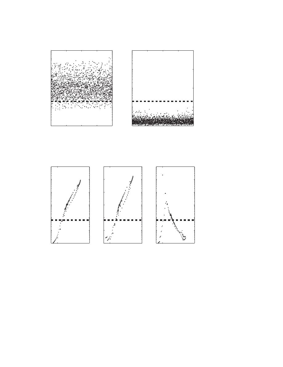
In Figure 7.1(a) we show the ratio of the normwise and componentwise eigen-

value condition numbers of the eigenvalues for 100 quadratic eigenvalue problems of

Copyright

© by SIAM. Unauthorized reproduction of this article is prohibited.

1334

TIMO BETCKE

500

1000

1500

2000

2500

3000

3500

4000

10

0

10

2

10

4

Eigenvalue number

κ

(λ

)/cond(

λ

)

(a) No scaling

1000

2000

3000

4000

10

0

10

2

10

4

Eigenvalue number

κ

(λ

)/cond(

λ

)

(b) Scaling,

ω=1

1000

2000

3000

4000

10

0

10

2

10

4

Eigenvalue number

κ

(λ

)/cond(

λ

)

(c) Scaling,

ω=|λ|

Fig. 7.1

. (a) The ratio of the normwise and componentwise condition numbers for the eigen-

values of 100 randomly created quadratic test problems of dimension n = 20 before scaling. (b) The
same test set but now after scaling with ω = 1. (c) Eigenvalue dependent scaling with ω =

|λ|.

dimension n = 20. The eigenvalues range in magnitude from 10

−8

to 10

8

and are

sorted in ascending magnitude. According to Theorem 3.3 the ratio of normwise
and componentwise condition number is smaller than n (shown by the dotted line)
if the problem is almost optimally scaled for the corresponding eigenvalue. But only
a few eigenvalues satisfy this condition. Hence, we expect that scaling will improve
the normwise condition numbers of the eigenvalues in these test problems. In Figure
7.1(b) the test problems are scaled using Alg. 1 with the fixed parameter ω = 1.
Apart from the extreme ones, all eigenvalues are now almost optimally scaled. In Fig-
ure 7.1(c) an eigenvalue dependent scaling is used; that is, ω = |λ| for each eigenvalue
λ. Now all eigenvalues are almost optimally scaled. This demonstrates that having
some information about the magnitude of the wanted eigenvalues can greatly improve
the results of scaling.

The source of badly scaled eigenvalue problems often lies in a nonoptimal choice

of units in the modelling process, which can lead to all coefficient matrices A

k

being

badly scaled in a similar way. In that case it is not necessary to provide any kind of
weighting. This is demonstrated by the example in Figure 7.2. The left plot in that
figure shows the ratio of the normwise and componentwise condition numbers of the
eigenvalues of another set of eigenvalue problems. Again, we choose n = 20 and = 2.
However, this time the matrices F

(k)

1

and F

(k)

2

in the definition A

k

:= F

(k)

1

˜

A

k

F

(k)

2

are

kept constant for all k = 0, . . . , . They vary only between different eigenvalue test
problems. The right plot in Figure 7.2 shows the ratio of normwise and componentwise
condition number after scaling using ω = 1. Now all eigenvalue condition numbers
are almost optimal.

Let us now consider the example of a 4th order PEP (λ

4

A

4

+ λ

3

A

3

+ λ

2

A

2

+

λA

1

+ A

0

)x = 0 derived from the Orr–Sommerfeld equation [16]. The matrices are

created with the NLEVP benchmark collection [1]. To improve the scaling factor ρ,
we substitute λ = μα

opt

, where α

opt

≈ 8.42 · 10

−4

. This reduces ρ from 1.99 · 10

12

to

4.86. The ratio κ

P

(μ)/cond

P

(μ) for the unscaled problem is shown in Figure 7.3(a).

Copyright

© by SIAM. Unauthorized reproduction of this article is prohibited.

SCALING OF EIGENVALUE PROBLEMS

1335

1000

2000

3000

4000

10

0

10

1

10

2

10

3

10

4

Eigenvalue number

κ

(λ

)/cond(

λ

)

(a) No scaling

1000

2000

3000

4000

10

0

10

1

10

2

10

3

10

4

Eigenvalue number

κ

(λ

)/cond(

λ

)

(b) Scaling,

ω=1

Fig. 7.2

. In this test all coefficient matrices of an eigenvalue problem are badly scaled in a

similar way. (a) Ratio of normwise and componentwise condition condition numbers before scaling.
(b) The same ratio after scaling with ω = 1.

10

0

10

5

10

0

10

1

10

2

10

3

10

4

10

5

10

6

|

μ|

κ

(μ

)/cond(

μ

)

(a) No scaling

10

0

10

5

10

0

10

1

10

2

10

3

10

4

10

5

10

6

|

μ|

κ

(μ

)/cond(

μ

)

(b) Scaling,

ω=1

10

0

10

5

10

0

10

1

10

2

10

3

10

4

10

5

10

6

|

μ|

κ

(μ

)/cond(

μ

)

(c) Scaling,

ω=10

3

Fig. 7.3

. Scaling of a 4th order PEP. (a) κ(μ)/cond(μ) for the unscaled PEP. (b) The same

ratio after scaling with ω = 1. (c) Scaling with ω = 10

3

. The horizontal lines denote the dimension

n = 64 of the PEP.

The x-axis denotes the absolute value |μ| of an eigenvalue μ. The horizontal line shows
the dimension n = 64 of the problem. The large eigenvalues in this problem are far
away from being optimally scaled. In Figure 7.3(b) we use Alg. 1 with the weighting
parameter ω = 1. This has almost no effect on the normwise condition numbers
of the eigenvalues. In Figure 7.3(c) we use ω = 10

3

. Now the larger eigenvalues

are almost optimally scaled while the normwise condition numbers of some of the
smaller eigenvalues have become worse. Hence, in this example the right choice of

Copyright

© by SIAM. Unauthorized reproduction of this article is prohibited.

1336

TIMO BETCKE

10

5

10

10

10

0

10

1

10

2

10

3

10

4

10

5

10

6

|

λ|

κ

(λ

)/cond(

λ

)

(a) No scaling

10

5

10

10

10

0

10

1

10

2

10

3

10

4

10

5

10

6

|

λ|

κ

(λ

)/cond(

λ

)

(b) Scaling,

ω=1

10

5

10

10

10

0

10

1

10

2

10

3

10

4

10

5

10

6

|

λ|

κ

(λ

)/cond(

λ

)

(c) Scaling,

ω=10

7

Fig. 7.4

. Scaling of the GEP Kx = λM x, where K and M are the matrices BCSSTK03 and

BCSSTM03 from Matrix Market [13]. The best overall results are obtained with ω = 10

7

(see right

graph). The horizontal lines denote the dimension n = 112 of the GEP.

the weighting parameter ω is crucial. If we want to improve the scaling of the large
eigenvalue, we need to choose ω as approximately the magnitude of these values
to obtain good results. By diagonal scaling with D

1

and D

2

the scaling factor ρ

might increase again. In this example, after diagonal scaling using the weight ω =
10

3

, ρ increases to 1.8 · 10

5

. However, we can reduce this again by another variable

transformation of the form μ = ˜

α

opt

˜

μ. From Theorem 6.1 it follows that ˜

α

opt

≈

13.9, and after this variable transformation ρ reduces to 67.6. Hence, at the end the
condition numbers of the largest eigenvalues have decreased by a factor of about 10

5

,

while the scaling factor ρ has increased only by a factor of about 10.

Not only for polynomial problems can a weighted scaling significantly improve the

condition numbers compared to unweighted scaling. In Figure 7.4 we show the results
of scaling for the GEP Kx = λM x, where K and M are the matrices BCSSTK03
and BCSSTM03 from Matrix Market [13]. The dimension of the GEP is 112. While
unweighted scaling improves the condition number of the smaller eigenvalues, the
best result is obtained by using the weighting parameter ω = 10

7

. Then the condition

number of all eigenvalues is improved considerably.

8. Some remarks about scaling in practice. In this concluding section we

want to give some suggestions for practical scaling algorithms based on the results of
this paper.

1. Compute κ(λ) and cond(λ) for each eigenvalue. At the moment eigensolvers

often return a normwise condition number if desired by the user. It is only a little more
effort to additionally compute the ratio κ(λ)/cond(λ). From Theorem 3.3 it follows
that a polynomial is almost optimally scaled for a certain eigenvalue if κ(λ)/cond(λ) ≤
n. If this condition is violated, the user may decide to rescale the eigenvalue problem
and then to recompute the eigenvalues in order to improve their accuracy.

2. Use a weighted scaling. The numerical examples in section 7 show that the

results of scaling can be greatly improved if ω is chosen to be of the magnitude of

Copyright

© by SIAM. Unauthorized reproduction of this article is prohibited.

SCALING OF EIGENVALUE PROBLEMS

1337

the wanted eigenvalues. In many applications this information is available from other
considerations. If no information about the eigenvalues is available, a reasonable
choice is to set ω = 1.

3. First linearize and then scale if no special structure of the linearization is

used. The results in section 4 show that one can obtain a smaller condition number if
one scales after linearizing the polynomial P (λ). If the eigenvalues of the linearization
L(λ) are computed without taking any special structure of L(λ) into account, this is
therefore the preferable way. However, if the eigensolver uses the special structure of
the linearization L(λ), then one should scale the original polynomial P (λ) and then
linearize in order not to destroy this structure.

4. Use a variable substitution of the type λ = αμ to reduce the scaling factor ρ.

This technique, which was introduced by Fan, Lin, and Van Dooren [3] for quadratics
and generalized in Theorem 6.1, often reduces the ratio of the condition number of
an eigenvalue λ between the linearization and the original polynomial. In practice we
would compute α using the Frobenius or another cheaply computable norm.

The first two suggestions also apply to generalized linear eigenvalue problems and

can be easily implemented to current standard solvers for them. Further research is
needed for the effect of scaling on the backward error. Bounds on the backward error
after scaling are difficult to obtain since the computed eigenvalues change after scaling
and this change depends on the eigensolver.

Acknowledgments. The author would like to thank Nick Higham and Fran¸coise

Tisseur for their support and advice on this work. Furthermore, the author would
like to thank the anonymous referees whose comments improved the paper.

REFERENCES

[1] T. Betcke, N. J. Higham, V. Mehrmann, C. Schr¨

oder, and F. Tisseur

, NLEVP: A col-

lection of nonlinear eigenvalue problems, MIMS EPrint 2008.40, Manchester Institute of
Mathematical Sciences, University of Manchester, 2008.

[2] T.-Y. Chen and J. W. Demmel, Balancing sparse matrices for computing eigenvalues, Linear

Algebra Appl., 309 (2000), pp. 261–287.

[3] H.-Y. Fan, W.-W. Lin, and P. Van Dooren, Normwise scaling of second order polynomial

matrices, SIAM J. Matrix Anal. Appl., 26 (2004), pp. 252–256.

[4] I. Gohberg, P. Lancaster, and L. Rodman, Matrix Polynomials, Academic Press, New York,

1982.

[5] D. J. Higham and N. J. Higham, Structured backward error and condition of generalized

eigenvalue problems, SIAM J. Matrix Anal. Appl., 20 (1998), pp. 493–512.

[6] N. J. Higham, R.-C. Li, and F. Tisseur, Backward error of polynomial eigenproblems solved

by linearization, SIAM J. Matrix Anal. Appl., 29 (2007), pp. 1218–1241.

[7] N. J. Higham, D. S. Mackey, and F. Tisseur, The conditioning of linearizations of matrix

polynomials, SIAM J. Matrix Anal. Appl., 28 (2006), pp. 1005–1028.

[8] N. J. Higham, A survey of componentwise perturbation theory in numerical linear algebra, in

Mathematics of Computation 1943–1993: A Half Century of Computational Mathematics,
W. Gautschi, ed., Proc. Sympos. Appl. Math. 48, AMS, Providence, RI, 1994, pp. 49–77.

[9] N. J. Higham, Accuracy and Stability of Numerical Algorithms, 2nd ed., SIAM, Philadelphia,

2002.

[10] D. Kressner, Numerical methods for general and structured eigenvalue problems, Lecture

Notes in Comput. Sci. Engrg. 46, Springer-Verlag, Berlin, 2005.

[11] D. Lemonnier and P. Van Dooren, Balancing regular matrix pencils, SIAM J. Matrix Anal.

Appl., 28 (2006), pp. 253–263.

[12] D. S. Mackey, N. Mackey, C. Mehl, and V. Mehrmann, Vector spaces of linearizations for

matrix polynomials, SIAM J. Matrix Anal. Appl., 28 (2006), pp. 971–1004.

[13] Matrix Market. http://math.nist.gov/MatrixMarket/.
[14] E. E. Osborne, On pre-conditioning of matrices, J. ACM, 7 (60), pp. 338–345.

Copyright

© by SIAM. Unauthorized reproduction of this article is prohibited.

1338

TIMO BETCKE

[15] B. N. Parlett and C. Reinsch, Balancing a matrix for calculation of eigenvalues and eigen-

vectors, Numer. Math., 13 (1969), pp. 293–304.

[16] F. Tisseur and N. J. Higham, Structured pseudospectra for polynomial eigenvalue problems,

with applications, SIAM J. Matrix Anal. Appl., 23 (2001), pp. 187–208.

[17] F. Tisseur, Backward error and condition of polynomial eigenvalue problems, Linear Algebra

Appl., 309 (2000), pp. 339–361.

[18] R. C. Ward, Balancing the generalized eigenvalue problem, SIAM J. Sci. Statist. Comput., 2

(1981), pp. 141–152.

[19] D. S. Watkins, A case where balancing is harmful, Electron. Trans. Numer. Anal., 23 (2006),

pp. 1–4.