Lecture 14: CUSUM and EWMA

Spanos

EE290H F05

1

CUSUM, MA and EWMA Control Charts

Increasing the sensitivity and getting ready for
automated control:

The Cumulative Sum chart, the Moving
Average and the Exponentially Weighted
Moving Average Charts.

Lecture 14: CUSUM and EWMA

Spanos

EE290H F05

2

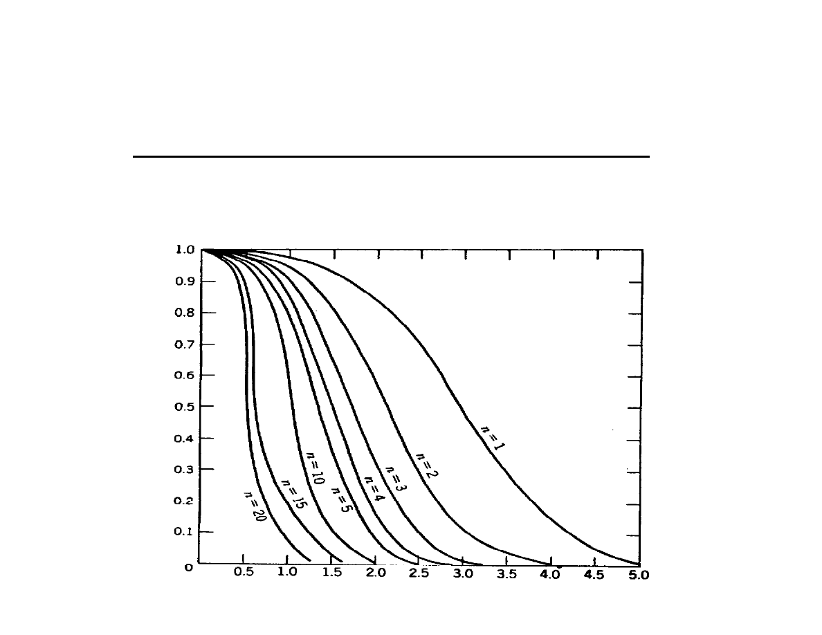
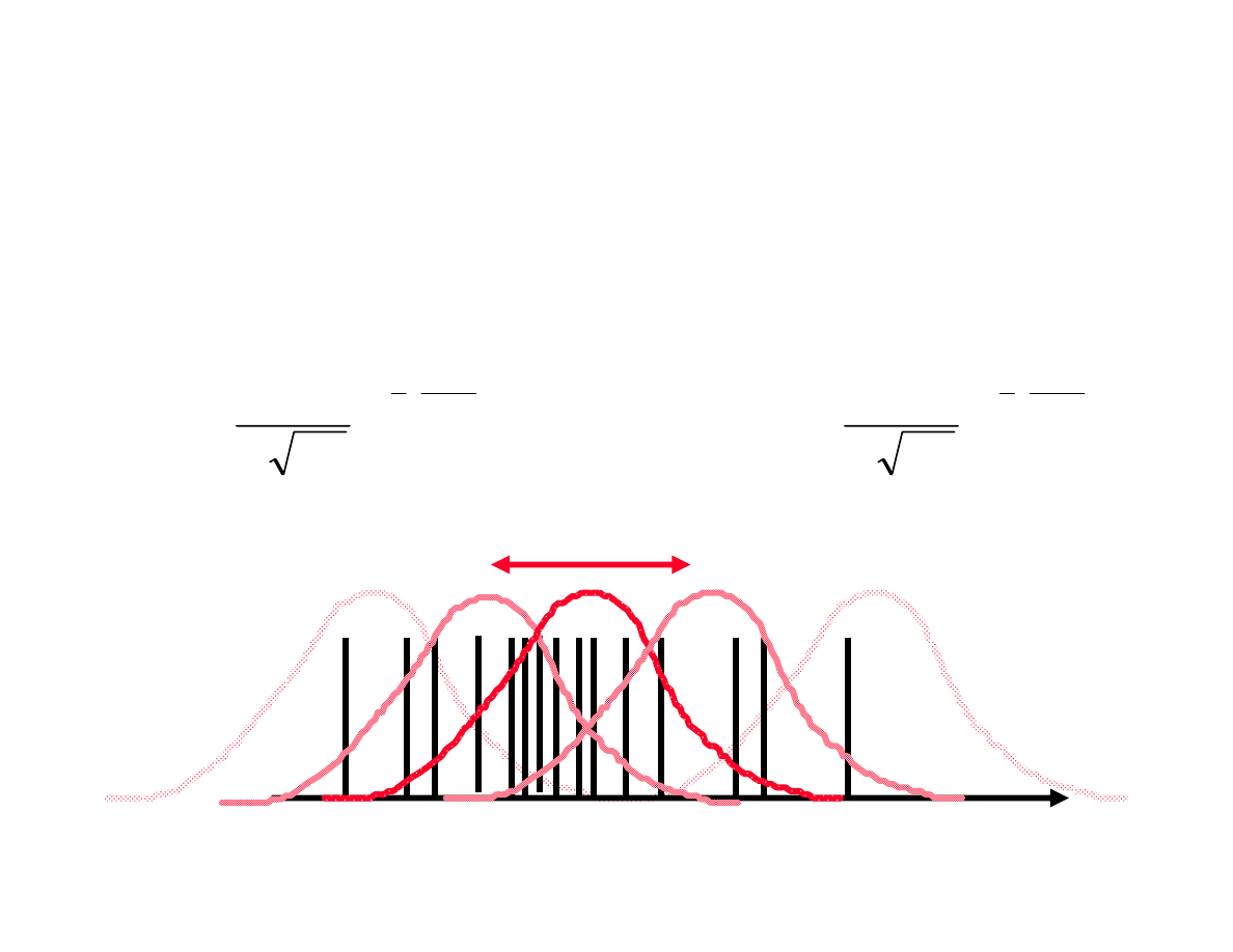
Shewhart Charts cannot detect small shifts

Fig 6-13 pp 195 Montgomery.

The charts discussed so far are variations of the Shewhart
chart: each new point depends only on one subgroup.

Shewhart charts are sensitive to large process shifts.

The probability of detecting small shifts fast is rather small:

Lecture 14: CUSUM and EWMA

Spanos

EE290H F05

3

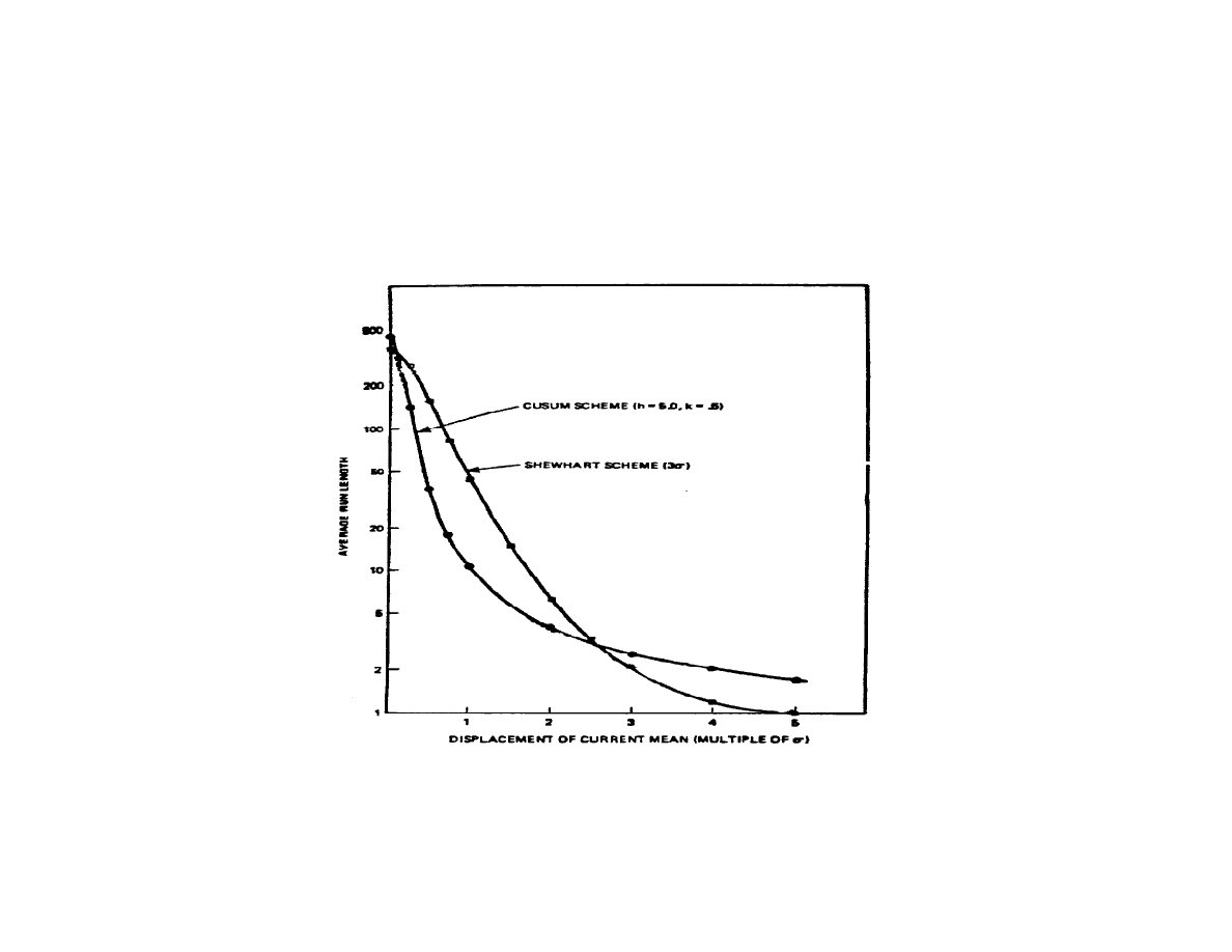
Cumulative-Sum Chart

If each point on the chart is the cumulative history (integral)
of the process, systematic shifts are easily detected. Large,
abrupt shifts are not detected as fast as in a Shewhart chart.

CUSUM charts are built on the principle of Maximum
Likelihood Estimation (MLE).

Lecture 14: CUSUM and EWMA

Spanos

EE290H F05

4

The "correct" choice of probability density function (pdf)
moments maximizes the collective likelihood of the
observations.

If x is distributed with a pdf(x,

θ) with unknown θ, then θ can

be estimated by solving the problem:

This concept is good for estimation as well as for comparison.

Maximum Likelihood Estimation

max

θ

m

Π

i=1

pdf( x

i

,

θ)

Lecture 14: CUSUM and EWMA

Spanos

EE290H F05

5

Maximum Likelihood Estimation Example

To estimate the mean value of a normal distribution, collect
the observations x

1

,x

2

, ... ,x

m

and solve the non-linear

programming problem:

⎪

⎪

⎭

⎪⎪

⎬

⎫

⎪

⎪

⎩

⎪⎪

⎨

⎧

⎟

⎟

⎠

⎞

⎜

⎜

⎝

⎛

Σ

⎪

⎭

⎪

⎬

⎫

⎪

⎩

⎪

⎨

⎧

Π

⎟

⎠

⎞

⎜

⎝

⎛ −

−

=

⎟

⎠

⎞

⎜

⎝

⎛ −

−

=

2

2

ˆ

2

1

1

ˆ

ˆ

2

1

1

ˆ

2

1

log

min

2

1

max

σ

μ

μ

σ

μ

μ

π

σ

π

σ

i

i

x

m

i

x

m

i

e

or

e

Lecture 14: CUSUM and EWMA

Spanos

EE290H F05

6

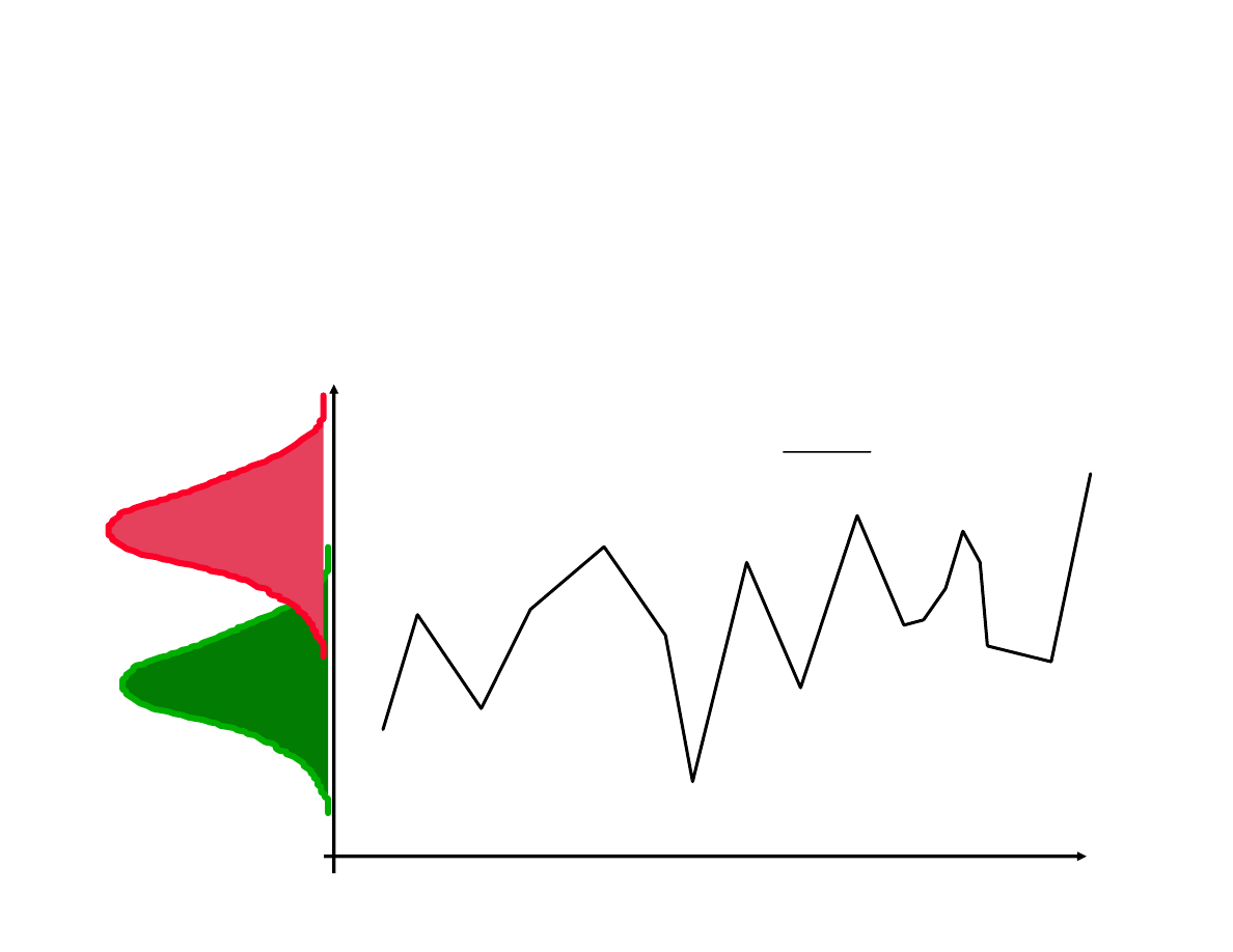
MLE Control Schemes

If a process can have a "

good

" or a "

bad

" state (with the control

variable distributed with a pdf f

G

or f

B

respectively).

This statistic will be small when the process is "

good

" and large when

"

bad

":

m

Σ

i=1

log

f

B

(x

i

)

f

G

(x

i

)

∑

=

=

=

Π

m

i

i

i

m

i

p

p

1

1

)

log(

)

log(

Lecture 14: CUSUM and EWMA

Spanos

EE290H F05

7

MLE Control Schemes (cont.)

S

m =

m

Σ

i=1

log

f

B

(x

i

)

f

G

(x

i

)

- min

k < m

k

Σ

i=1

log

f

B

(x

i

)

f

G

(x

i

)

> L

or

S

m

= max (S

m-1

+log

f

B

(x

m

)

f

G

(x

m

)

, 0) > L

Note that this counts from the beginning of the process. We
choose the best k points as "calibration" and we get:

This way, the statistic S

m

keeps a cumulative score of all the

"bad" points.

Notice that we need to know what the "bad"

process is!

Lecture 14: CUSUM and EWMA

Spanos

EE290H F05

8

The Cumulative Sum chart

S

m

=

m

Σ

i=1

(x

i

- µ

0

)

Advantages

The CUSUM chart is very effective for small shifts and
when the subgroup size n=1.

Disadvantages

The CUSUM is relatively slow to respond to large shifts.
Also, special patterns are hard to see and analyze.

If

θ is a mean value of a normal distribution

,

is simplified to:

where

μ

0

is the target mean of the process. This can be

monitored with V-shaped or tabular “limits”.

Lecture 14: CUSUM and EWMA

Spanos

EE290H F05

9

Example

-15

-10

-5

0

5

10

15

20

40

60

80

100

120

140

160

µ0=-0.1

LCL=-13.6

UCL=13.4

-60

-40

-20

0

20

40

60

80

100

120

0

20

40

60

80

100

120

140

160

0

Shewhart

small shift

CUSUM small shift

Lecture 14: CUSUM and EWMA

Spanos

EE290H F05

10

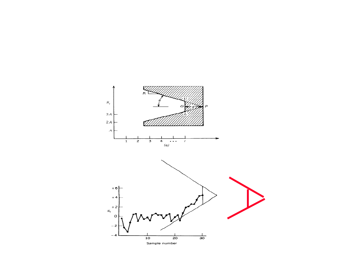
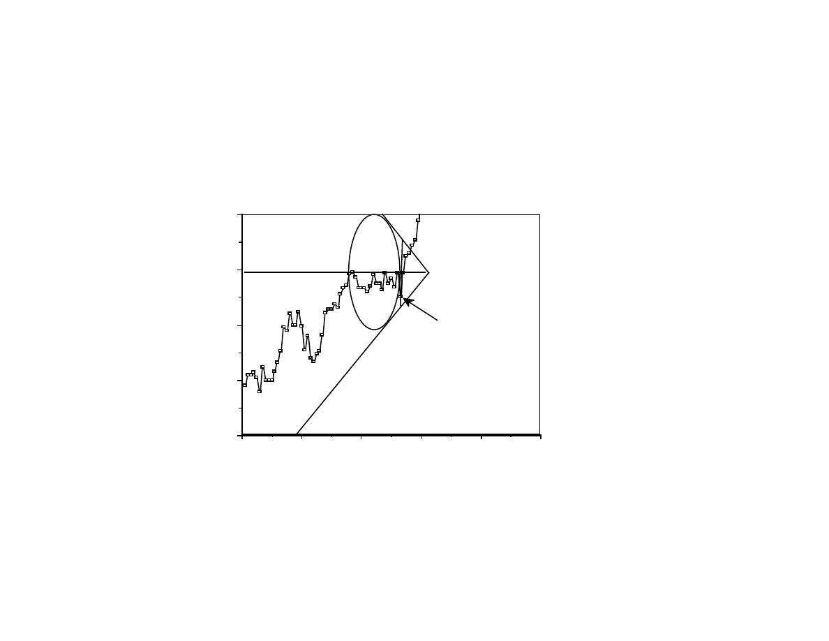
The V-Mask CUSUM design

for standardized observations y

i

=(x

i

-

μ

o

)/

σ

Figure 7-3 Montgomery pp 227

Need to set

L(0)

(i.e. the run length when the process is in

control), and

L(

δ)

(i.e. the run-length for a specific deviation).

Lecture 14: CUSUM and EWMA

Spanos

EE290H F05

11

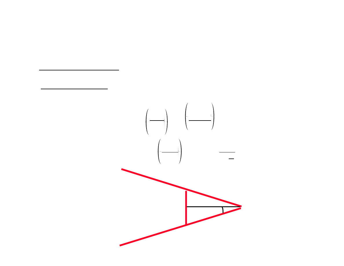
The V-Mask CUSUM design

for standardized observations y

i

=(x

i

-

μ

o

)/

σ

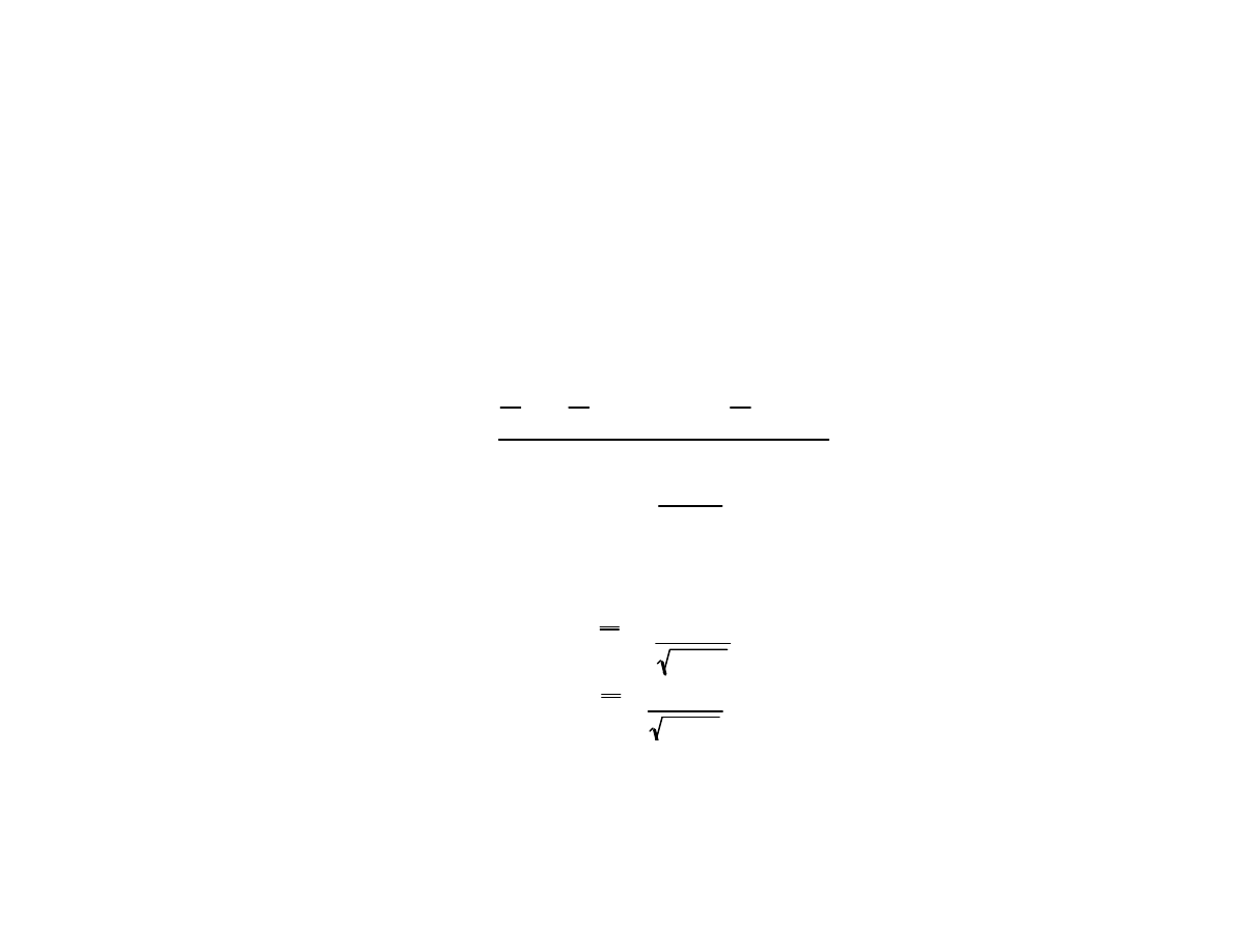
d = 2

δ

2

ln

1-

β

α

θ = tan

-1

δ

2A

δ = Δ

σ

x

d

θ

δ is the amount of shift (normalized to σ) that we wish to detect with type I
error

α and type II error β.

Α is a scaling factor: it is the horizontal distance between successive
points in terms of unit distance on the vertical axis.

Lecture 14: CUSUM and EWMA

Spanos

EE290H F05

12

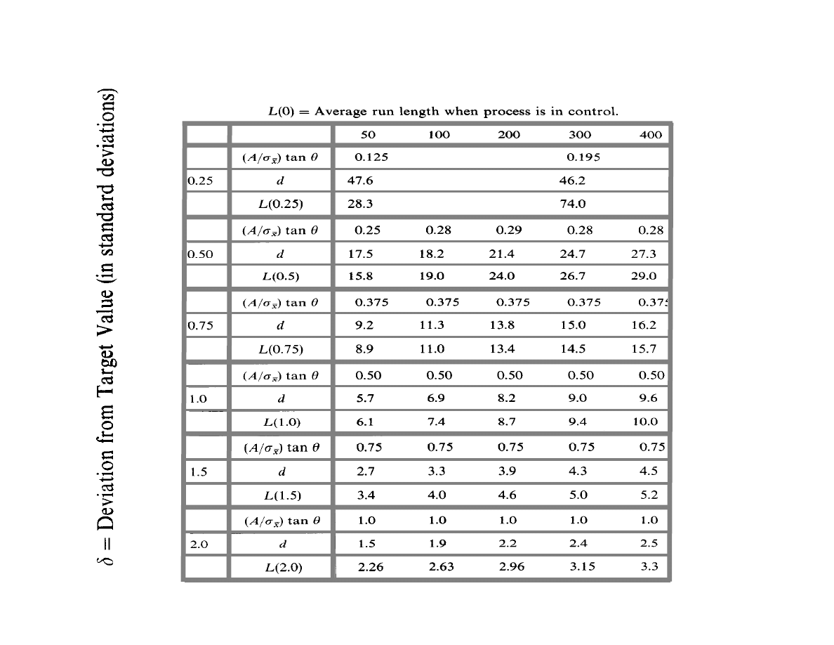
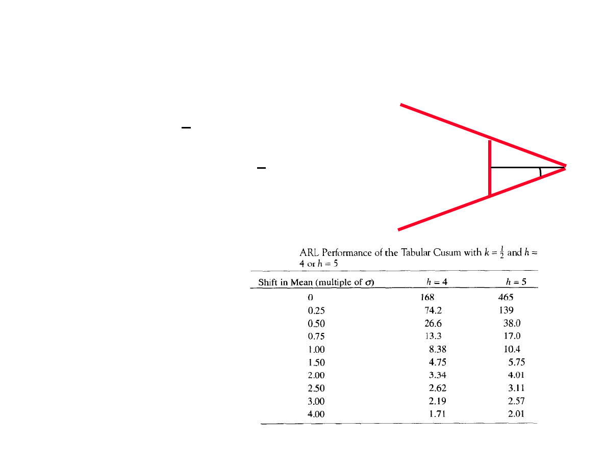
ARL vs. Deviation for V-Mask CUSUM

Lecture 14: CUSUM and EWMA

Spanos

EE290H F05

13

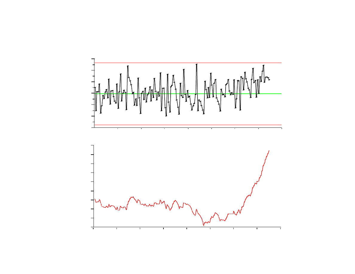
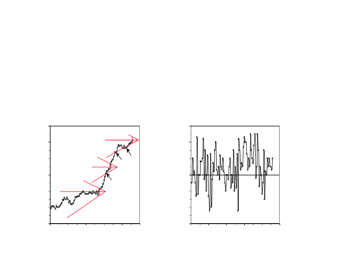
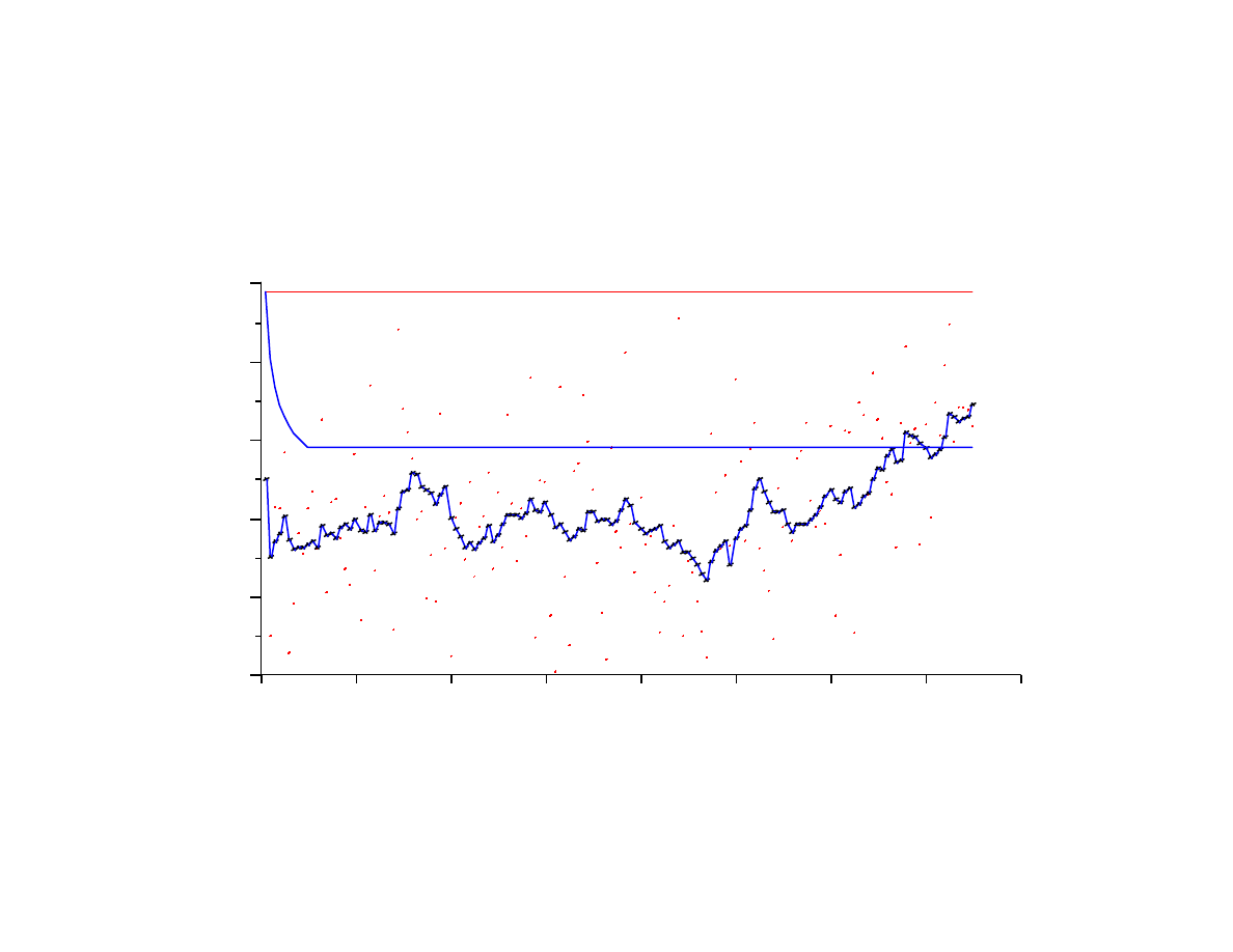
CUSUM chart of furnace Temperature difference

I

II

III

Detect 2C

o

,

σ =1.5C

o

, (i.e.

δ=1.33), α=.0027 β=0.05,

A=1

=>

θ = 18.43

o

, d = 6.6

100

80

60

40

20

0

-10

0

10

20

30

40

50

100

80

60

40

20

0

-3

-2

-1

0

1

2

3

Lecture 14: CUSUM and EWMA

Spanos

EE290H F05

14

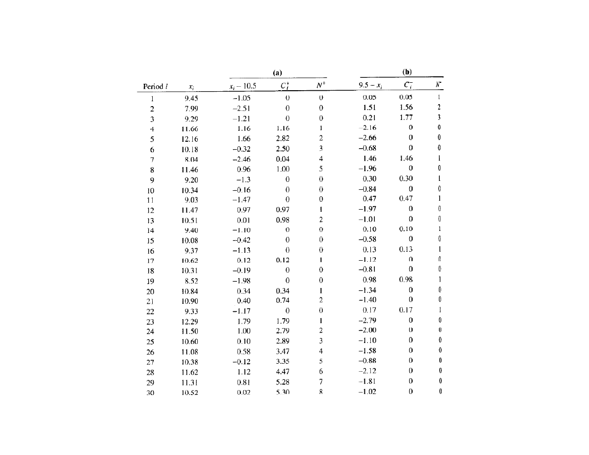
Tabular CUSUM

A tabular form is easier to implement in a CAM system

C

i

+

= max [ 0, x

i

- (

μ

o

+ k ) + C

i-1

+

]

C

i

-

= max [ 0, (

μ

o

- k ) - x

i

+ C

i-1

-

]

C

0

+

= C

0

-

= 0

k = (

δ/2)/σ

h = d

σ

x

tan(

θ)

d

θ

h

Lecture 14: CUSUM and EWMA

Spanos

EE290H F05

15

Tabular CUSUM Example

Lecture 14: CUSUM and EWMA

Spanos

EE290H F05

16

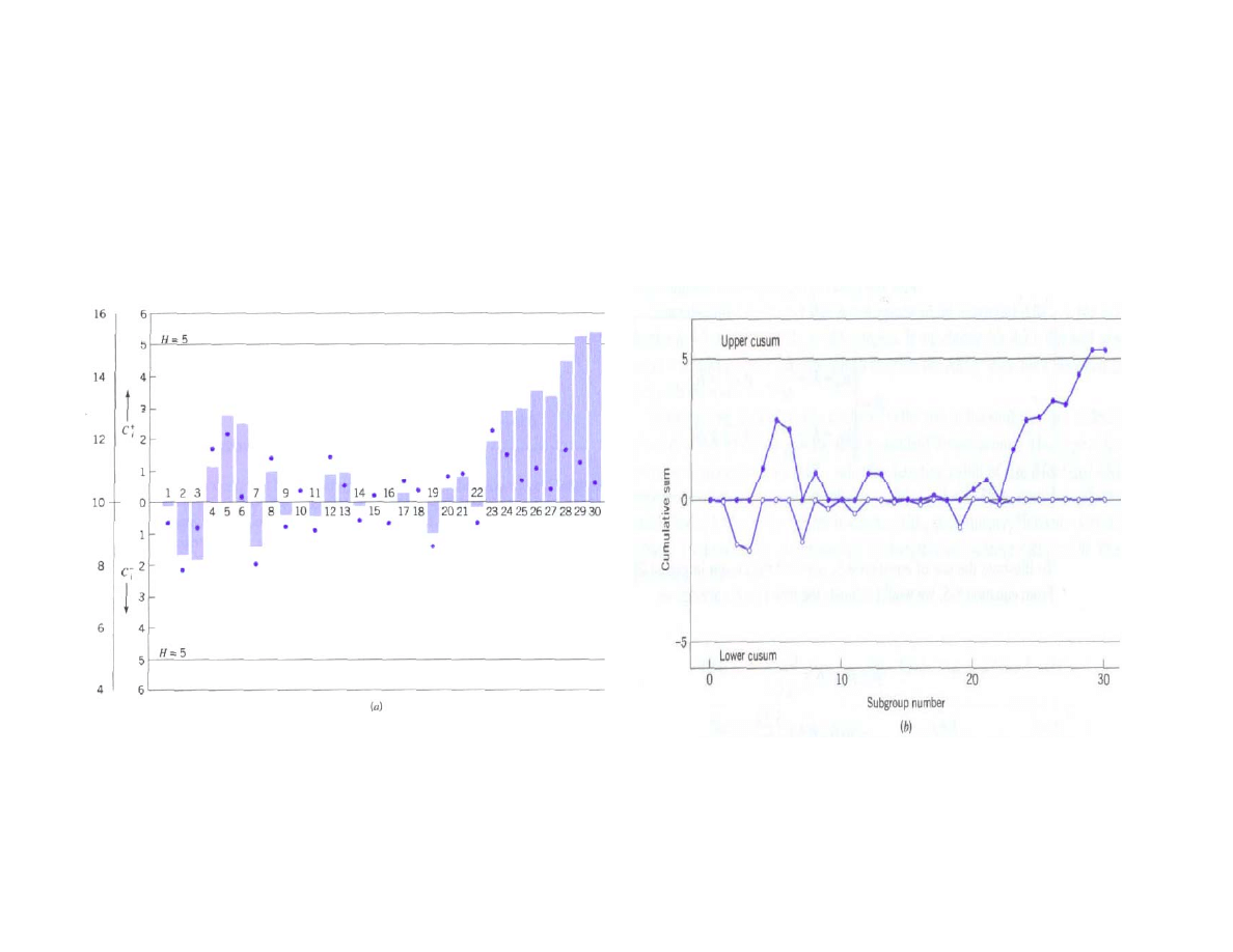
Various Tabular CUSUM Representations

Lecture 14: CUSUM and EWMA

Spanos

EE290H F05

17

CUSUM Enhancements

Other solutions include the application of Fast Initial
Response (FIR) CUSUM, or the use of combined CUSUM-
Shewhart charts.

To speed up CUSUM response one can use "modified" V
masks:

100

80

60

40

20

0

-5

0

5

10

15

Lecture 14: CUSUM and EWMA

Spanos

EE290H F05

18

General MLE Control Schemes

Since the MLE principle is so general, control
schemes can be built to detect:

• single or multivariate deviation in means

• deviation in variances

• deviation in covariances

An important point to remember is that MLE
schemes need, implicitly or explicitly, a definition of
the "

bad

" process.

The calculation of the ARL is complex but possible.

Lecture 14: CUSUM and EWMA

Spanos

EE290H F05

19

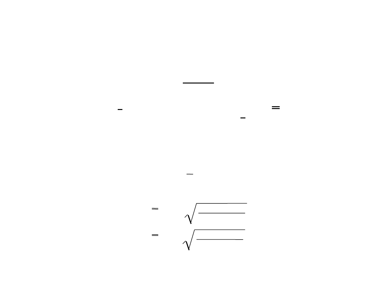
Control Charts Based on Weighted Averages

The 3-sigma control limits for M

t

are:

M

t

=

x

t

+ x

t-1

+ ... +x

t-w+1

w

V(M

t

) = σ

2

n w

UCL = x + 3 σ

n w

LCL = x - 3 σ

n w

Small shifts can be detected more easily when multiple
samples are combined.

Consider the average over a "moving window" that contains
w subgroups of size n:

Limits are wider during start-up and stabilize after the first w
groups have been collected.

Lecture 14: CUSUM and EWMA

Spanos

EE290H F05

20

Example - Moving average chart

-10

-5

0

5

10

15

0

20

40

60

80

100

120

140

160

sample

w = 10

Lecture 14: CUSUM and EWMA

Spanos

EE290H F05

21

The Exponentially Weighted Moving Average

If the CUSUM chart is the sum of the entire process history,
maybe a weighed sum of the recent history would be more
meaningful:

z

t

=

λx

t

+ (1 -

λ)z

t -1

0 <

λ < 1 z

0

= x

It can be shown that the weights decrease geometrically
and that they sum up to unity.

z

t

=

λ

( 1 -

λ )

j

x

t - j

+ ( 1 -

λ )

t

z

0

Σ

j = 0

t - 1

UCL

=

x

+

3

σ

λ

( 2 -

λ ) n

LCL

=

x

-

3

σ

λ

( 2 -

λ ) n

Lecture 14: CUSUM and EWMA

Spanos

EE290H F05

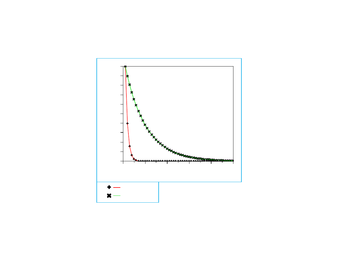
22

Two example Weighting Envelopes

0.0

0.1

0.2

0.3

0.4

0.5

0.6

0.7

0.8

0.9

1.0

0

10

20

30

40

50

EWMA 0.6
EWMA 0.1

-> age of sample

relative
importance

Lecture 14: CUSUM and EWMA

Spanos

EE290H F05

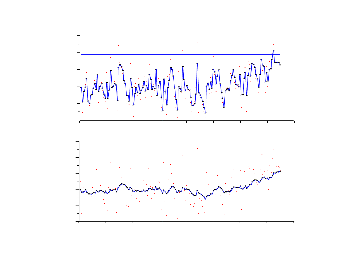
23

EWMA Comparisons

-10

-5

0

5

10

15

0

20

40

60

80

100

120

140

160

sample

-10

-5

0

5

10

15

0

20

40

60

80

100

120

140

160

λ=0.6

λ=0.1

Lecture 14: CUSUM and EWMA

Spanos

EE290H F05

24

Another View of the EWMA

• The EWMA value z

t

is a forecast of the sample at the t+1

period.

• Because of this, EWMA belongs to a general category of

filters that are known as “time series” filters.

• The proper formulation of these filters can be used for

forecasting and feedback / feed-forward control!

• Also, for quality control purposes, these filters can be used

to translate a non-IIND signal to an IIND residual...

x

t

= f ( x

t - 1

, x

t - 2

, x

t - 3

,... )

x

t

- x

t

= a

t

Usually:

x

t

=

φ

i

x

t - i

Σ

i = 1

p

+

θ

j

a

t - j

Σ

j = 1

q

Lecture 14: CUSUM and EWMA

Spanos

EE290H F05

25

Summary so far…

While simple control charts are great tools for visualizing
the process,it is possible to look at them from another
perspective:

Control charts are useful “summaries” of the process
statistics.

Charts can be designed to increase sensitivity without
sacrificing type I error.

It is this type of advanced charts that can form the
foundation of the automation control of the (near) future.

Next stop before we get there: multivariate and model-
based SPC!