
1
(DDPS)
DIDACTIC AND DIGITAL
PHOTOGRAMMETRIC SOFTWARE
User’s Guide


3
INTRODUCTION
This program was developed within the framework of a cooperative project between
the SURFACES Laboratory, Department of Geomatics, University of Liege and the
Institute of Geodesy and Cartography (IGiK), Department of Photogrammetry ,
Poland.
Our main objective is to produce a complete and integrated educational
photogrammetric package. The graphic interface was made with a didactical
objective, rapid as possible and easy to understand. The final result is a very user-
friendly interface. No special knowledge is needed (except in photogrammetry) for
using the software.

4
POSSIBILITIES AND FUNCTIONNALITIES OF THE SOFTWARE
1. REQUIREMENTS AND POSSIBILITIES
1.1.Requirements
Digital Photogrammetric Software
processes digital images with 8 bits/pixel (grey
level). File format is BMP.
The images must be photographs taken with a metric camera for that characteristics
are known. So the user must have at one's disposal the calibration certificate of the
camera.
To enable the absolute orientation of the photos, a sufficient number of control points
discernible on the two photos must be known.
1.2.Possibilities
A complete photogrammetric treatment is possible with Digital Photogrammetric
Sofware. The following general workflow can be use to realise it:
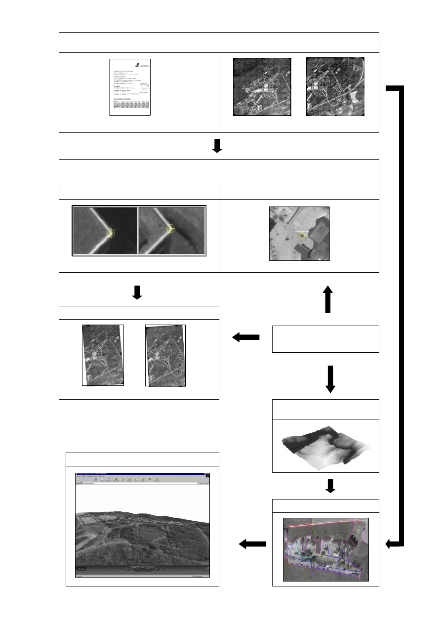
5
INNER
ORIENTATION
Pixel coordinates => Photo coordinates
Calibration Certificate
Left Image
Right Image
EXTERIOR ORIENTATION
RELATIVE ORIENTATION ABSOLUTE ORIENTATION
Photo coordinates => Model coordinates Model coordinates => Ground coordinates
Homologous points
Control points
EPIPOLAR
RESAMPLING
Determination of the bounding box
IMAGE MATCHING
GENERATION OF THE
DEM
ORTHORECTIFICATION
VRML MODEL GENERATION
6
2. TO MOVE IN THE IMAGES
The views of the different steps of the photogrammetric orientation (inner, relative
and absolute orientation) are organised in three different views of the same image.
1
1
3
3
1
2
3
2
2
The view 1 is the over view that shows the entire image.
The view 2 corresponds to the original size of the image and is the part of the view 1
included in the white rectangle.
The view 3 is a detail view that shows the part of the image within the white rectangle
of the view 2.
When you want to track down a point in the image, place the cursor in the view 1
near by this point and click on the right mouse button. The white rectangle is then
centred on the selected point and the part of the image included inside appears in the
view 2. Next do the same thing with the view 2 to locate more accurately the point.
3. TO TRACK DOWN POINTS IN THE IMAGES
Before tracking down a point in the image, you must select the line of the current
point in the chart below the image. Then the cursor becomes a hair cross.
Points can
be selected in all the three views. To be more accurate, it’s better to
locate it in the view 3 (refer at 2: to move in the images)
When you have adjusted the view on the point, place the centre of the hair cross on
this. Then click two times on the left mouse button to select the point. The image
coordinates appear on the correspondent line of the chart below the image. . When
the hair cross isn’t just on the point, it can be moved by holding the left mouse button
and move the mouse.
INNER ORIENTATION
RELATIVE AND ABSOLUTE
ORIENTATION
7
4. TO MOVE IN THE CHARTS
Some additional functions have been added to make easier the displacements in the
relative and absolute orientations charts.
After the selection of the current line (by clicking on this in the chart with the left
mouse button), you can move from line to line or laterally with the help of the
direction arrows of the keyboard.
5. TO MAKE A ZOOM
It’s possible to increase or decrease the size of the white rectangle in the views 1 and
2, modifying in this way respectively the views 2 and 3.
After the selection of the view within you want to make the zoom, click concurrently
on Alt and * to decrease the zoom and on Alt and / to increase it. Then the view of
the superior level will automatically change.
6. THE THREADS
Sometimes, by mistake or inexperience, the user can choose parameters that lead to
process the data for long time. In this case, it’s useful to know how many times the
process will take.
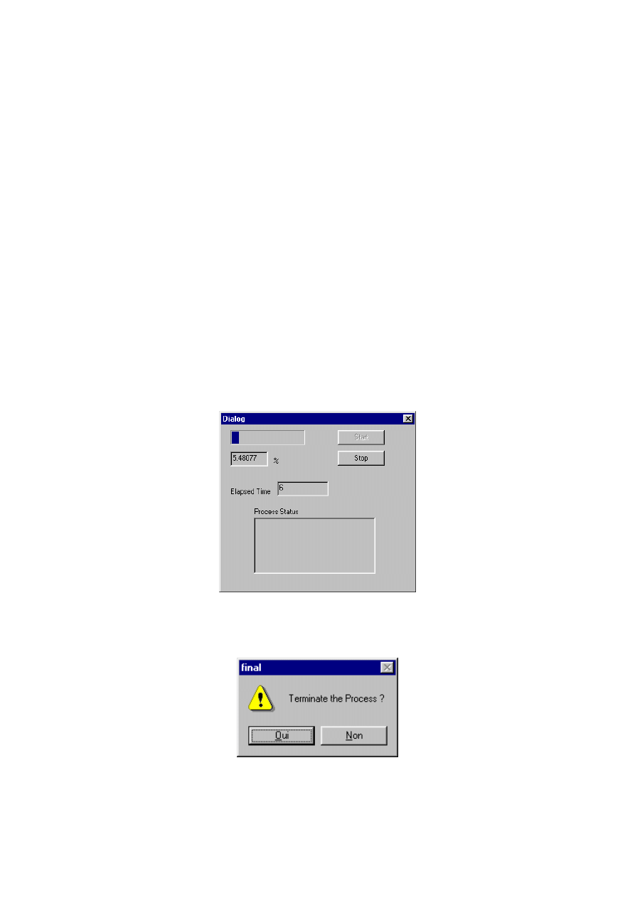
The thread is useful for estimating the duration of a specific task.
Another interesting functionality is that a process putted in a thread can be
interrupted at each time the user wants.
8
DATA PROCESSING
1.INNER ORIENTATION
An inner orientation must be done for every image. This process allows establishing
a relation between the pixel and image coordinates. This relation is determined with
the help of the fiducial marks photo coordinates given in the calibration certificate
(see annex 1).
To change the pixel coordinates into photo coordinates, you must encode the values
of the photo coordinates of the fiducial marks. Then a parallel between these values
and the pixel coordinates will can be drawn.
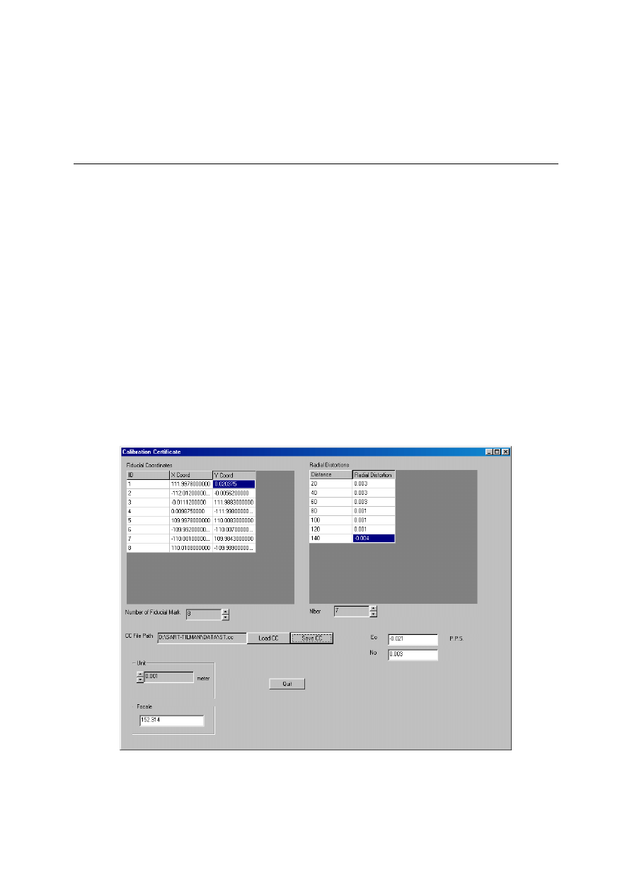
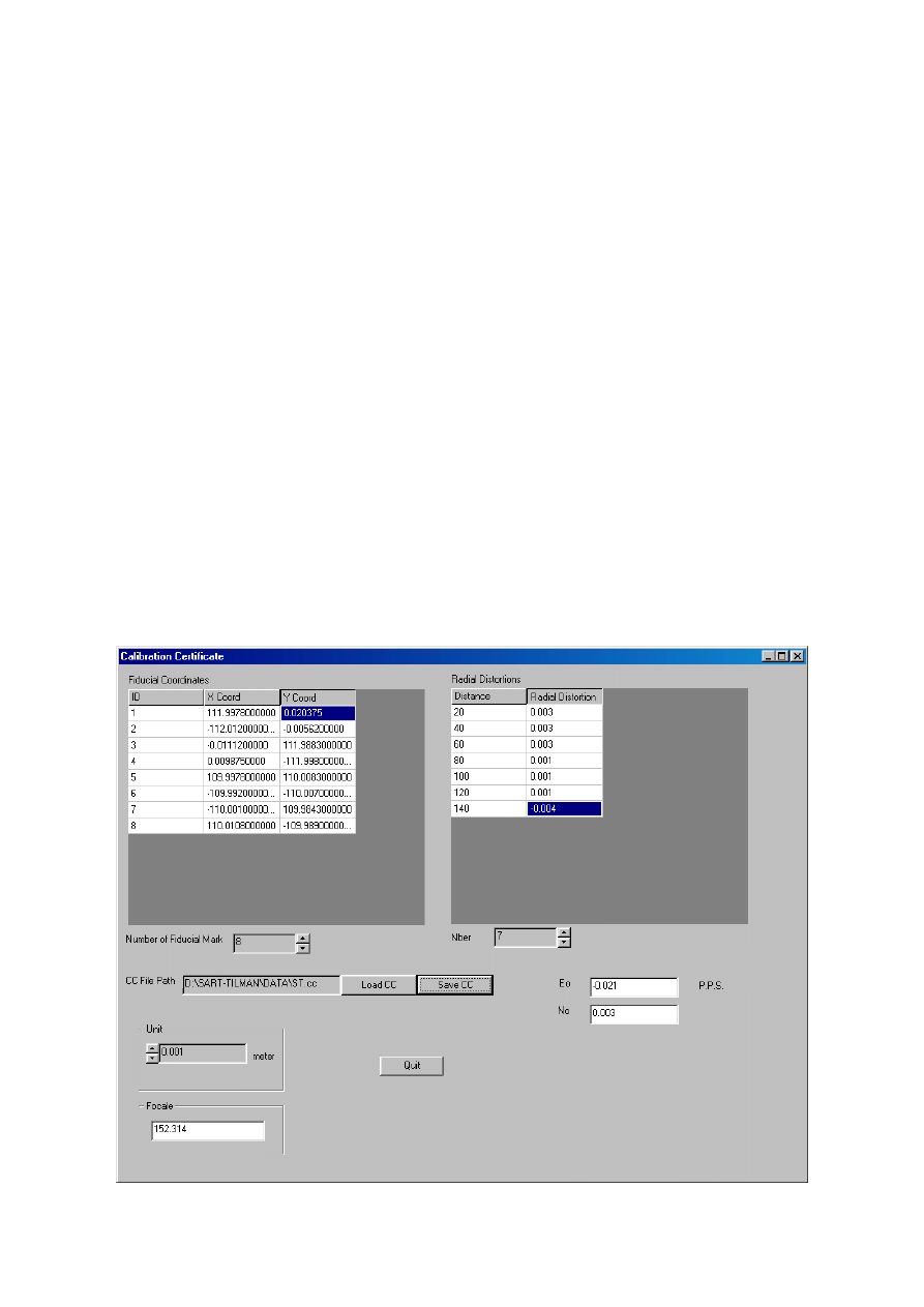
Encode the calibration certificate
A. The camera has never been encoded.
In the project window, choose the option New CC. The following dialog box will pop
up:
The first thing to do is the choice of the units, that will be the units used in all the
project. For more facilities, the units can be these of the calibration certificate. With

9
the help of the arrows on the left of the case called Unit, you can increase or
decrease the value of the units. When you have determined it, you must think that all
the values will be expressed in these units.
The following step is the encoding of the values that you have in the calibration
certificate:
- f focal length: the value must be written in the Focale case
- PP position of the principal point:
The value of
0
corresponds to the E
0
case
The value of
0
corresponds to the N
0
case
- position of the fiducial marks:
The superior part of the left window is devoted to receive the photo coordinates of
the fiducial marks. By clicking on the arrows below the chart can you determinate
the number of fiducial marks. Next, the ID, X Coord and Y Coord (corresponding
to the photo coordinates) of every fiducial marks can be encoded.
- lens distortion:
The superior part of the right window is devoted to receive the values of the lens
distortion. You can also determinate the number of radial distance and mean
radial distortion values by clicking on the arrows on the left of the case. Then the
chart can be completed with the radial distances in the left column and the mean
radial distortions in the right column.
All these informations can be saved in a “.cc” file with the option save CC or by
answering YES at the
question “Do you want to SAVE Calibration Certificate?” when
you quit.
B. The camera is the same that these that has already been encoded for precedent
photos.
Then the calibration certificate previously encoded can be got back. Click on Load
CC in the CC File Path case and take the appropriate file.
Location of fiducial marks
Now that the photo coordinates of the fiducial marks are known, the parameters of
the transformation of the pixel coordinates will be computed. Those will depend of
two things: the pixel coordinates values of the fiducial marks and the orientation of
the X and Y axes.
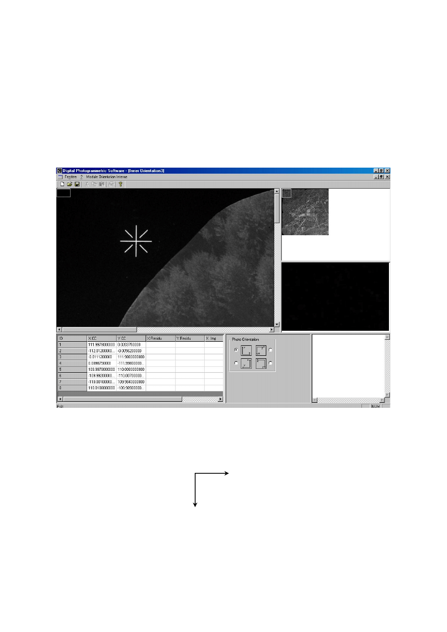
In the project window, choose the option Left or Right IO to make the inner
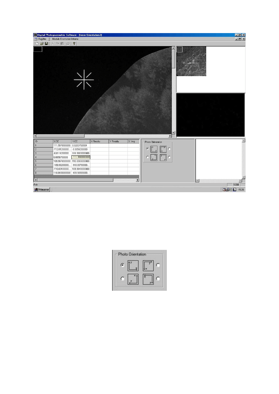
orientation of every one. The following window will appear:
10
There are three views of the same image. The right superior view is the over view
that shows the entire image. The left view corresponds to the original size of the
image. The right inferior view is a detail view that shows the part of the image within
the cursor of the left view.
The first step is the determination of the photo orientation. According to it, the
parameters of transformation will change. You have the choice between four cases.
This step will transform the start system in the ideal case (see the theory about this
part)
In the chart below the image, you find in the two first columns the values of the photo
coordinates given in the calibration certificate. The pixel coordinates are directly
registered in the XImg and YImg columns when you track down the fiducial marks on
every image. To move and locate points on the image, see the section
Functionnalities of the software.
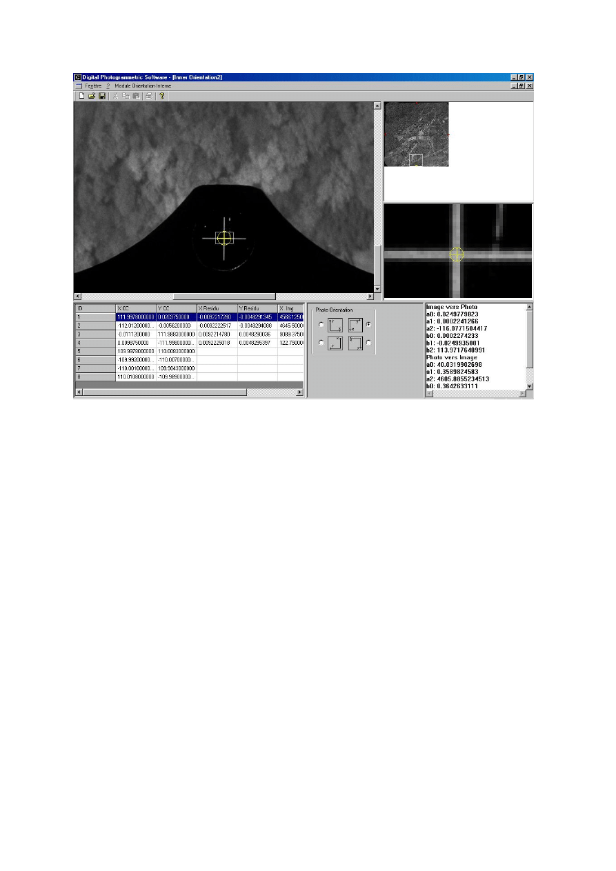
11
Parameters of transformation will appear as from three fiducial marks and residues
as from four fiducial marks.
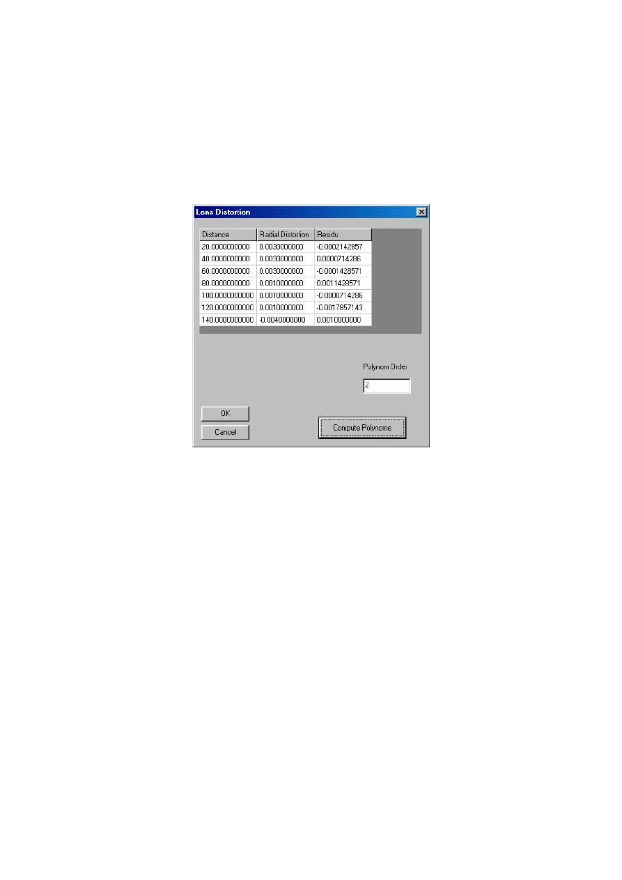
Correction of the radial lens distortion
In the menu Inner orientation module, choose the Radial Distortion option. The
window in that the parameters of the polynome are computed will pop up:
In this window, the values of the radial distances and of the mean radial distortions
previously encoded will automatically appear. You have the possibility to choose the
polynomial order but it must be less than the number of associated radial distances
and mean radial distortions. The you can compute the polynomial, in the third
column appear the residues.
2. EXTERIOR ORIENTATION
2.1. Relative orientation by rotations
Relative orientation allows determining the relative positions of the two bundles of
rays by creating spatial stereomodel in an arbitrary coordinate system. Tracking
down homologous points on the left and right images is necessary to make this
orientation.
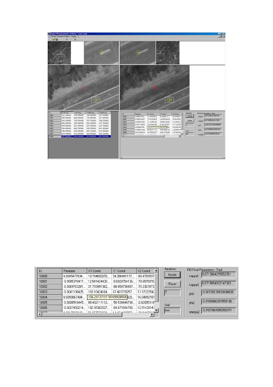
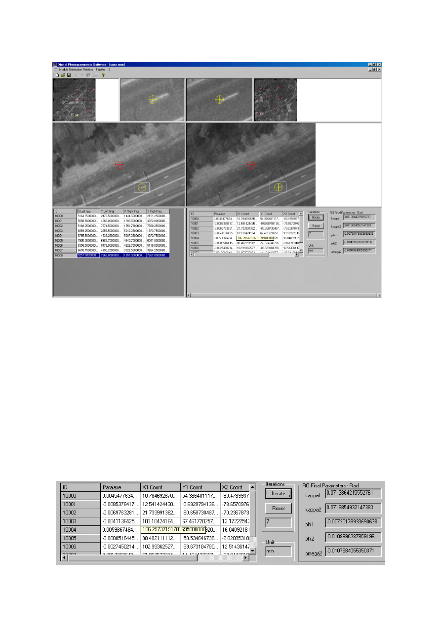
In the project window, click on the button RO by Rotations. The following window
box will appear:
12
By clicking with the right mouse button on a grey case of the chart under the left
image, you can choose to add a point with the option Add Point. Then you must
track down the homologous point on the left and right images: The left and right
image coordinates of the point will appear in the current line of the chart
It is possible to delete one point by clicking on the ID with the right mouse button and
by choosing the option Delete This Point.
As from five homologous points, it is possible to have values of RO Final Parameters
(expressed in Radians) by clicking on Reset the first time and after Iterate. Then
values of the chart will change: the parallax will decrease, new RO Final Parameters
are computed and new model coordinates (X
i
Coord, Y
i
Coord) are computed for every
image. Stop the iterations when you think that the parallax values are small enough
and that RO Final parameters don’t significantly change.
13
2.2. Absolute orientation
The purpose of absolute orientation is the transformation from model coordinates to
ground coordinates. To realise it, you must have points that ground coordinates are
known. These points are called the control points (CTRL) and will serve to the
computing of the parameters allowing the transformation from model coordinates to
ground coordinates.
Another type of points is the checkpoint (CHECK). It corresponds to points that
ground coordinates are known but that are not used for the computing of the absolute
orientation parameters. The residues on these points give an idea on the global
accuracy.
Last type is the tie point (TIE). It corresponds to points that ground coordinates are
unknown and for that ground coordinates are computed with the absolute orientation
parameters.
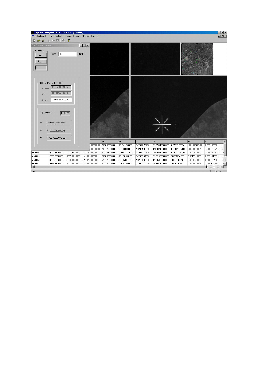
In the project window, click on AO & Restitution. Then appears the window of the
absolute orientation
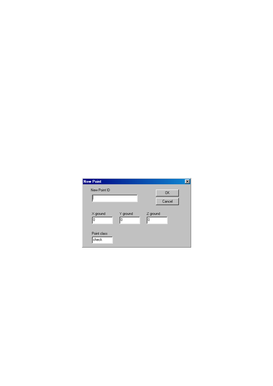
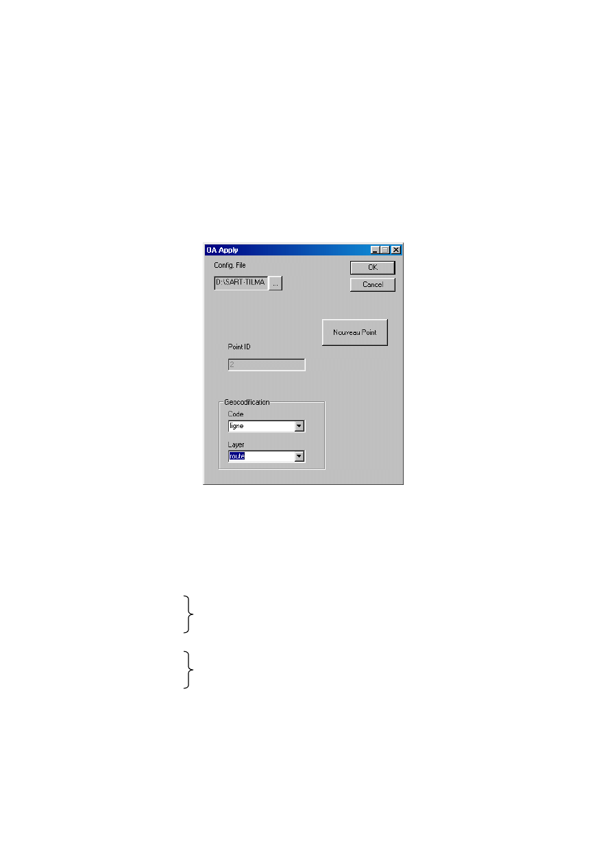
As for the relative orientation, you can add or delete points by clicking on the right
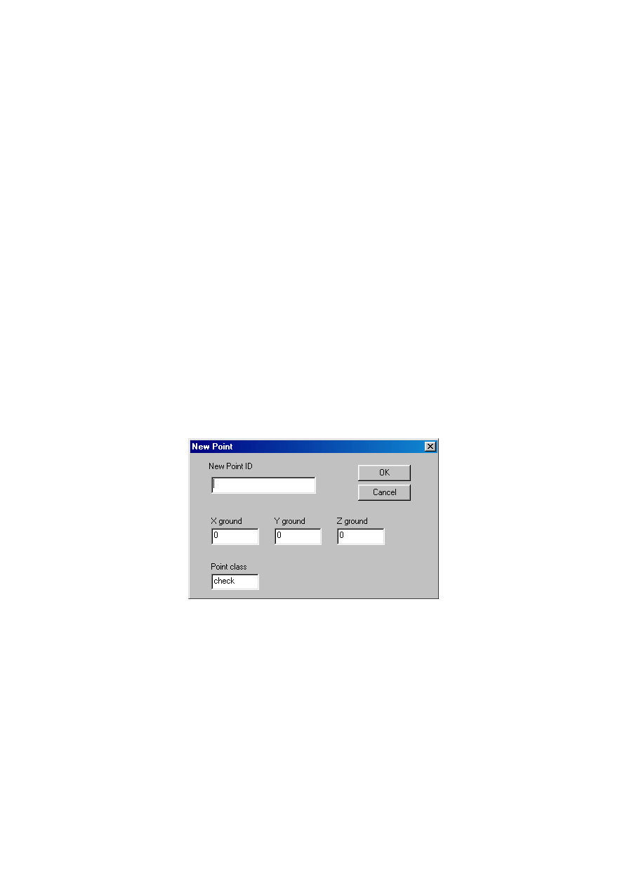
mouse button when you are in the chart.. The following window will appear:
This window allows the encoding of the control, the check and the tie points. In the
point class, write ctrl for control points, check for checkpoints and tie for tie points.
When ground coordinates of the current point are known, they can be encoded in this
chart. Coordinates can also be encoded in the general chart below the image by
selecting the correspondent case.
When points are located, control points appear in blue, checkpoints in green and tie
points in red. As for three control points, absolute orientation parameters can be
computed by clicking on Reset and then Iterate.
Stop the iterations when the residues on the control and checkpoints are small
enough (in the window, the residues are expressed in the same units that the units of
the check and control points). The values of the absolute orientation parameters are
in the grey window.
14
The value of the base has no importance; it will only change the value of the scale
factor.
The angle κ must sometimes be changed. Indeed, the first value of this angle is
calculated with the two first control points. In accordance with the relative position of
these points, you obtain the value of the κ-angle or of (π-κ). If the computed value is
(π-κ), residues will increase. Either you inverse the two first control points or just
after clicking Reset, change the given value by (π-κ) and then Iterate.
15
3. RESTITUTION
3.1. Monoscopic Restitution
In the project window, click on AO & Restitution - menu Module option Application.
This module allows to track down additional points for that ground coordinates are
unknown and to compute their ground coordinates with the absolute orientation
parameters. For the location of the homologous points, proceed in the same way
that for the others modules. The ground coordinates of the new points will directly
appear. These points will receive the type resti points.
3.2. Geo
– Coding
Create a Configuration File (.cl) that has the following structure (ex: tess.cl):
BEGIN_CODES
point
line
spline
END_CODES
BEGIN_LAYERS
road
hedge
fence
END_LAYERS
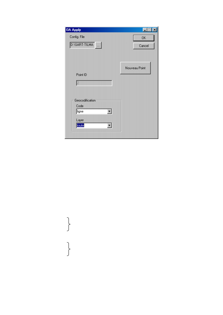
Then you choose for every point its code and its layer. A file with the ID, the type, the
layer, the code and the coordinates of the points is created. This file can directly be
employed in topographic programs.
you put here all the layers that you want to use
you put here all the codes that you want to use
16
3.3. Image Matching techniques
In the project window, click on AO & Restitution - menu Configuration option Auto
Find
– ON
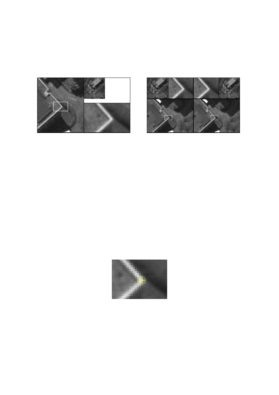
This module allows the automatic detection on the right image of the homologous
point tracked down on the left image.
In this program, an area based matching is used to identify the homologous points.
This method works with pattern, target and search window. Points are associated if
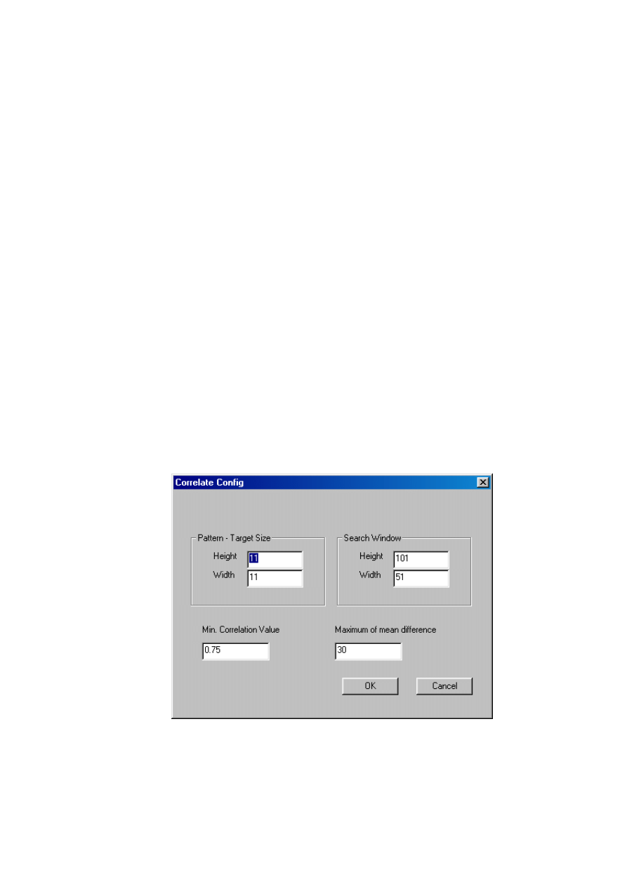
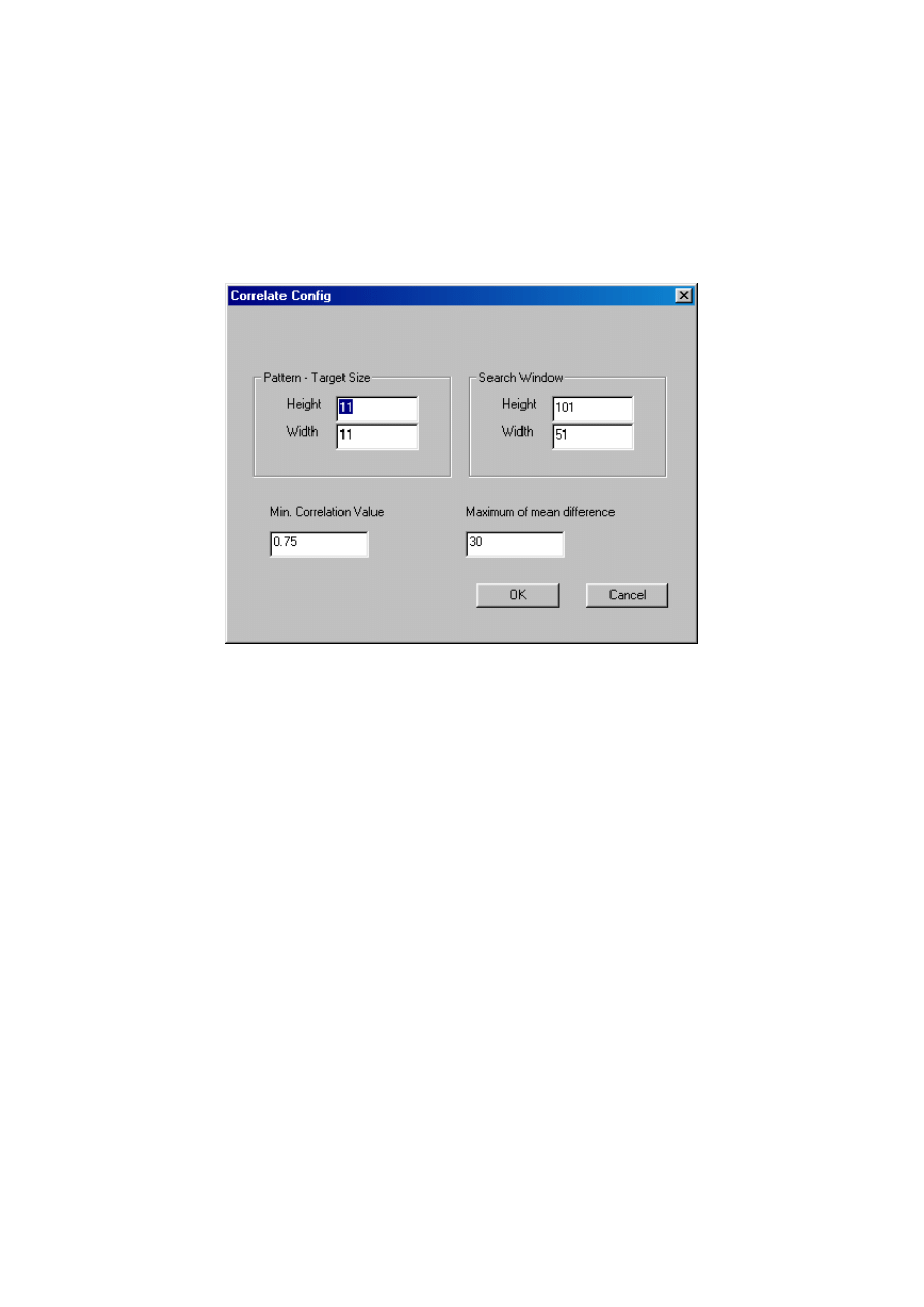
they have similar grey values. Before starting, you must configure the parameters of
the matching. The parameters of the matching that you can change are:
The size of the pattern and target window: there are the windows surrounding the
matched pixel
The size of the search window: the search window contains the matched pixels for
which correlation coefficients are computed
The minimum correlation value: if this value isn’t reached, the window “not
correlation” will appear and the cursor will be on an approximate position of the
homologous point.
The maximum of mean difference
When you have chosen to activate the auto-correlation, the homologous point on the
right image of the left image current point will automatically appear in the right
window. Sometimes the program can’t find the homologous point and then sends the
message “No Correlation”. Sometimes the point is not exactly the homologous of this
17
of the left image. In these two cases, you have always the possibility to displace the
point on the two images or to delete it. When the two points are tracked down, their
ground coordinates are computed in accordance with the absolute orientation
parameters.
4. EPIPOLAR RESAMPLING
The resolution of the created image can also be chosen. This parameter will
determinate its size in Ko.
Empty images are then created. Every point in these images undergoes inverse
transformation to catch in the original image its grey value.
Epipolar images have only horizontal parallaxes. These images offer the big
advantage to simplify the automatic correlation procedure, because it works in a
single direction.
4.1. Application
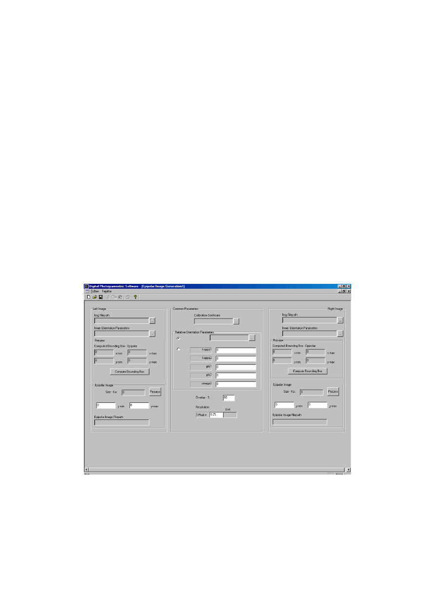
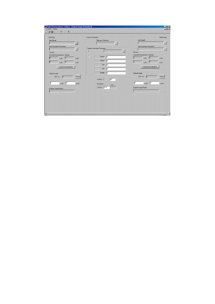
In the project window, click on Epipolar Images. The following dialog box will pop
up:
Load the necessary files.
Click on Compute Bounding Box to have the limits of this. These limits can be
changed. The X-limits depend on the overlay. The user can directly change the Y-
limits.
18
The options are:
you can choose to use the relative orientation parameters or put other values
for dω
2
, dφ
1
, dφ
2
, dκ
1
, and dκ
2
. Indeed, this module is completely independent
of the rest of the treatment and can be used with values found by another
program.
the overlay that will change the x min value of the left image and the x max
value of the right image
the resolution that will determinate the size of the created epipolar image (the
size appear above the y min and y max values).
When all these parameters are fixed, click on Process. You must directly give a
name and a File Path for the created image.
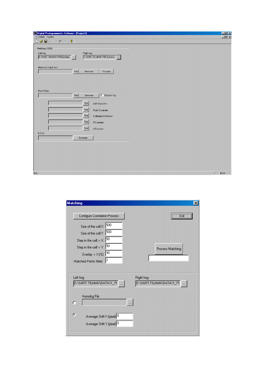
5. IMAGE MATCHING
5.1. Application
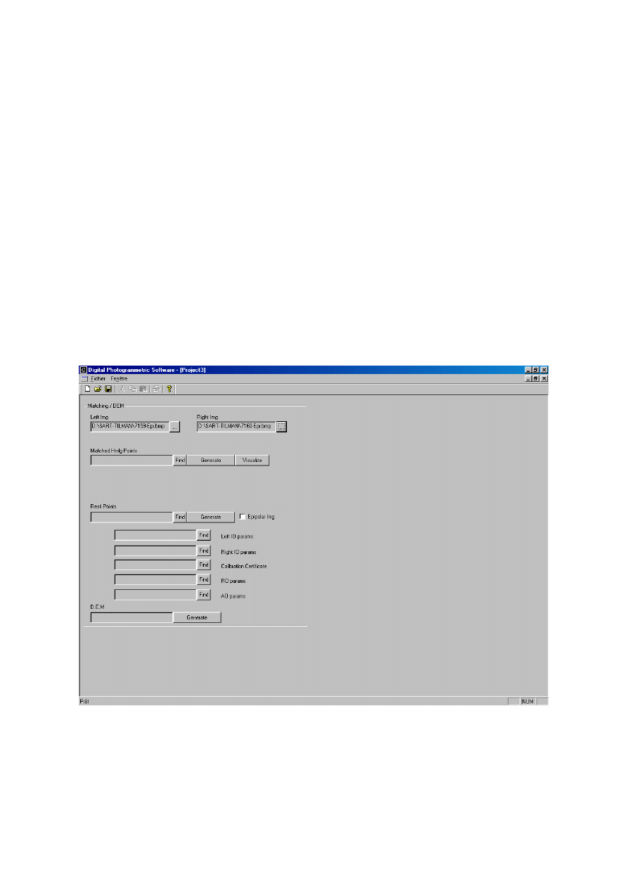
In the project window, click on Matching:
First choose the two images on which the matching is made. Indeed, image
matching can be made on the original images or on the epipolar images. In
accordance with the chosen images, the parameters of configuration can differ.
Click on Generate in the Matched Hmlg Points part. A dialog box allowing the
configuration of the matching will appear:
19
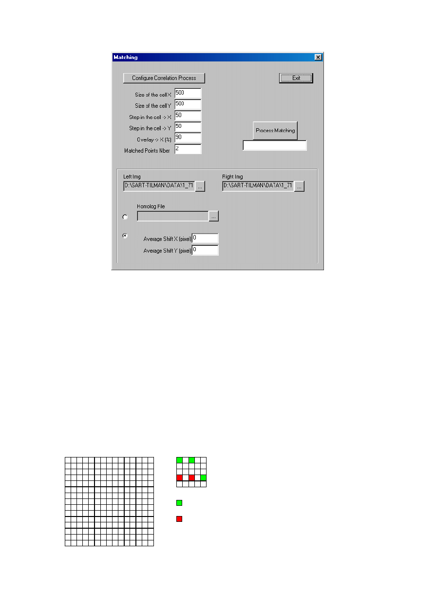
When you click on Configure Correlation Process, the same window that in the
automatic detection of homologous points will appear (see the absolute orientation to
configure it).
The superior part of the window contains various parameters:
Size of the cell: The chosen images are broken down into several cells in that
homologous points are searched.
Step in the cell is the number of points that it increments when homologous points
are found
Matched Points Nbr is the number of matched points that must be find in each
cell. As soon as this number is reached, points are computed in the following cell.
These three parameters must be chosen in accordance with the desired number of
matched points.
Overlay
Original image (15*15)
Matched point
Non-matched point
Example :
Size of the cell X :5
Size of the cell Y :5
Step in the cell X :2
Step in the cell Y :3
Matched Points Nbr : 3
20
For the predicted position of homologous points, there are two options:
Loading a homolog file; the predicted position are calculated in accordance with
the relative positions of the previously tracked down points.
Computing an average shift X and Y values in pixels. The shift values are given
by the respective differences between the X and Y image coordinates of two
homologous points. For one computed point in the left image, the homologous
point on the right image will be search in a zone displaced of the shift X and shift
Y values compared with the position on the left image.
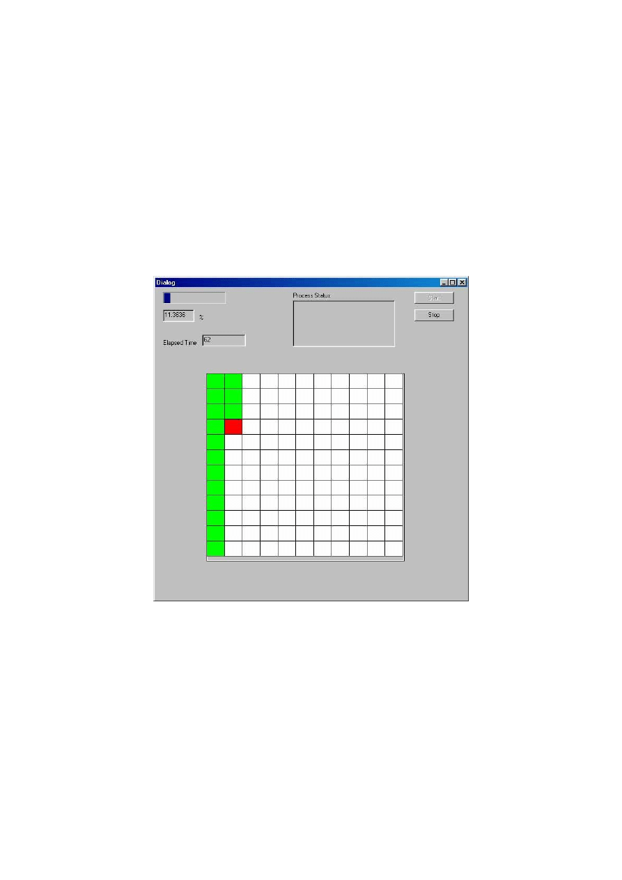
When all these parameters are fixed, click on Process Matching. A window informs
you on the course of the.process:
The under graph shows the cells within homologous points are searched. If the cell
remains green, then a sufficient number of homologous points for that the correlation
coefficient is sufficient have been found. If the cell remains red, then a number
inferior to the number asked by the user have been found.
When the matching is finished, it is possible to visualize the matched points by
clicking Visualize. This module allows deleting eventual non-homologous points. To
delete these points, click on its ID and press Del.
N.B: It is also possible to visualize a file with already matched points by clicking on
Find and by choosing the adequate file.
21
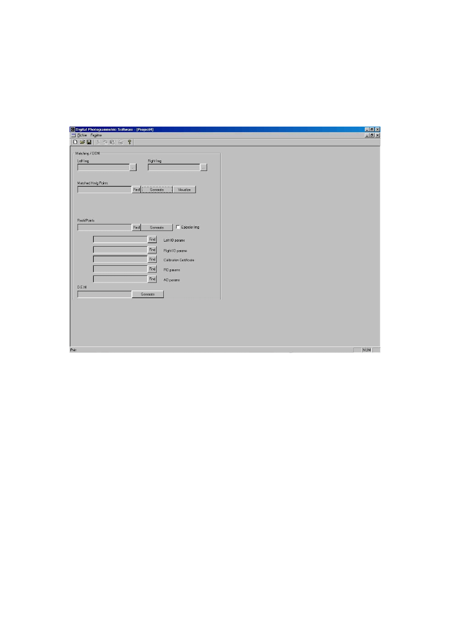
6. GENERATION OF THE DIGITAL ELEVATION MODEL (DEM)
6.1. Application
In the project window, click on Matching. The following window will appear:
For generating a DEM, you need a file containing ground coordinates. To have this
file, either load an already OAApply file by clicking on Find or generate a new file
with Generate. This new file is generated as from an hmlg file that must be load in
the Matched Hmlg Points case.
The hmlg file can be constituted of homologous points tracked down on the epipolar
images
– then mark the Epipolar Img case – or of homologous points tracked down
on the original images:
For the epipolar images, you must load the cc and OAparam files.
For the original images, you must load the Left and Right OIparam, cc,
ORparam and OAparam files.
When the OAApply file is loaded or generated, you can click on Generate in the DEM
part. The DEM config window will appear:
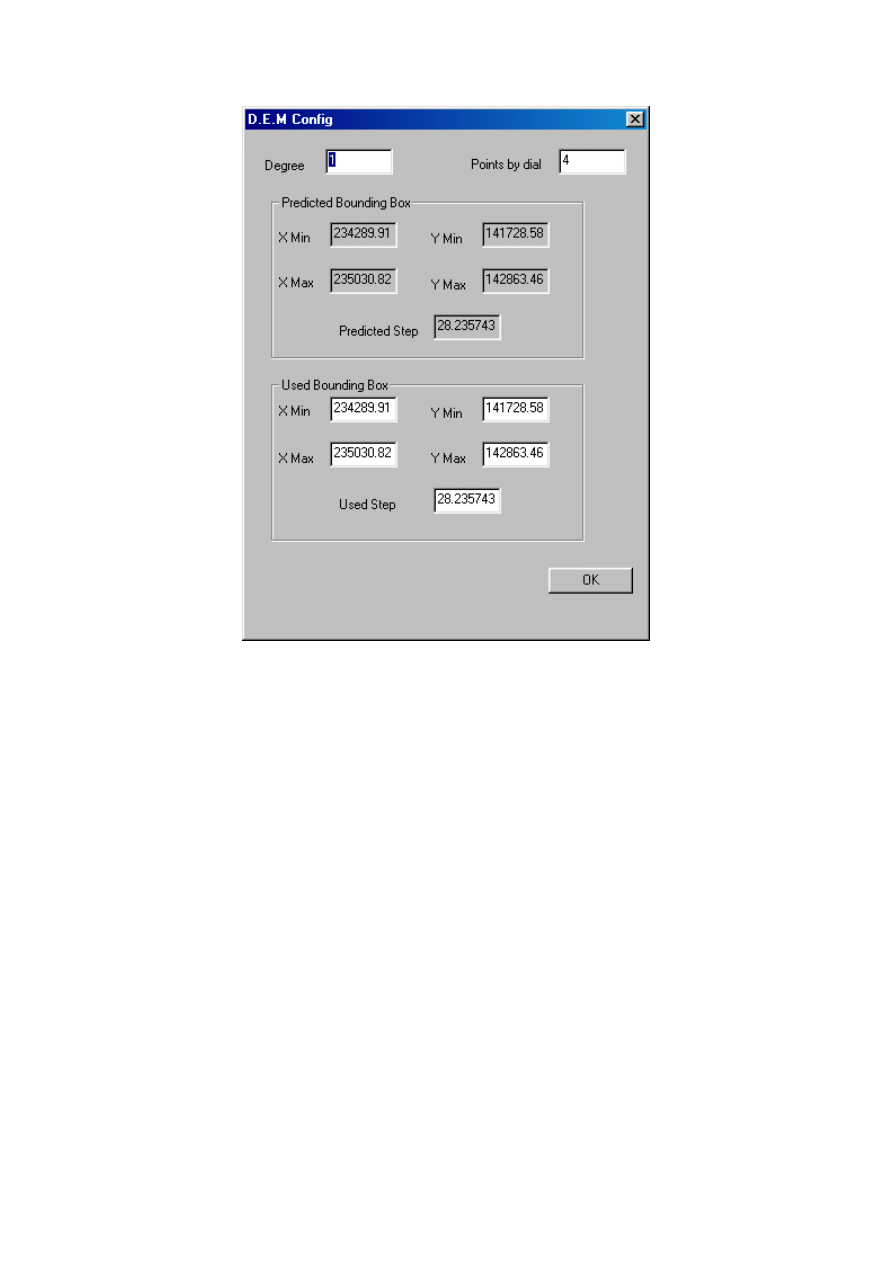
22
The predicted values that are proposed correspond respectively to:
degree of elevation is 1. So the distance is elevated at the degree 1. The fact of
increasing the degree of elevation allows to reduce the importance of the points
that are more far of the evaluated point.
the number of points by dial is 4. This number depends of the already determined
points and their distribution.
the bounding box is the framework built on the points the ground coordinates of
which are known. The user can change the area of the DEM if he wants to make
the DEM only within a part of the original image. He musts then enter the ground
coordinates of the X and Y minimum and maximum of the desired area. It is also
possible to make a DEM on a larger area but the points, which are out of the
framework, will be less accurate because they have
n’t known points in each
direction surrounding them.
the mean of the distance between each point known in the ground coordinates
and its nearest neighbour. This distance can be increased to accelerate the
procedure if few points are desired. It can be also reduced if the DEM must be
more accurate.
23
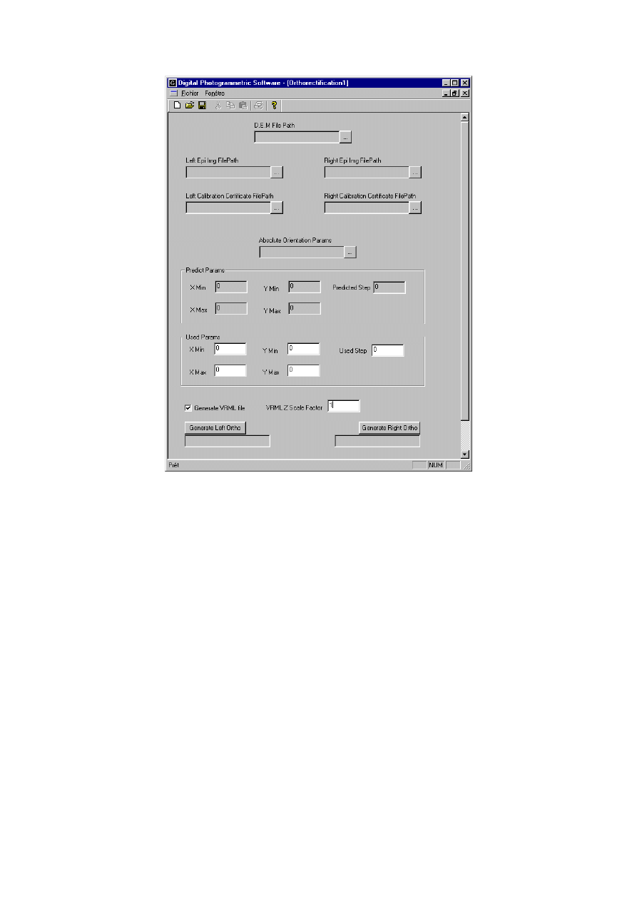
7. ORTHORECTIFICATION
7.1. Application
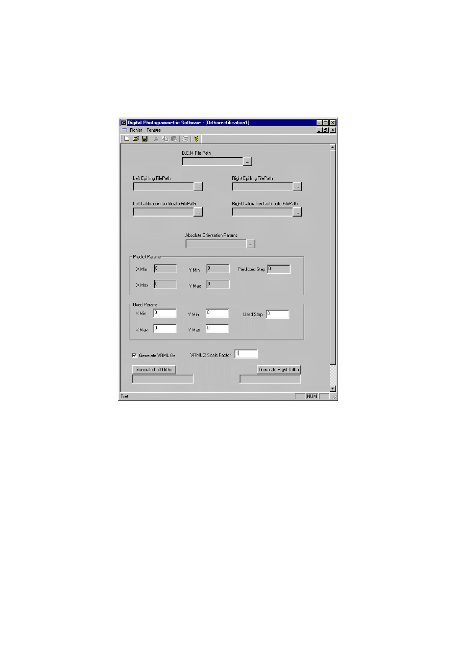
In the project window, click on Ortho:
To construct the orthophotograph, dem file, epipolar images, cc and OAparam files
must be loaded.
The first step is the choice of the future orthophotograph size. The default size given
by the program is the size of the area covered by the DEM. This can be changed but
must have limits inferior of those of the DEM. The predicted step corresponds also to
the step of the DEM. This factor will determine the resolution of the orthophotograph.
For every point in the orthophotograph, the DEM case in that it is localised is
computed. The Z value of the current point is then interpolated with a bilinear
interpolation.
Every point in the photograph must also receive the grey value of the corresponding
pixel in the epipolar image. This operation is realised by a transformation of the
24
ground coordinates into the epipolar coordinates. The current pixel receives the grey
value of the corresponding pixel of the epipolar image.
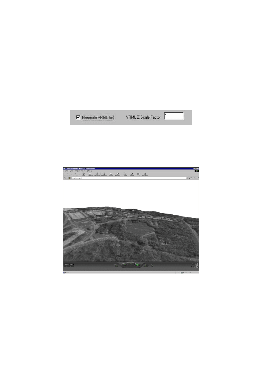
8. VRML MODEL GENERATION AND VISUALIZATION
The Virtual Reality Modeling Language allows to represent every 3D space with a
sufficient reality.
So it’s possible to have a view of the DEM draped with the orthophoto by activating
the option Generate VRML file in the Ortho module. The user chooses the Z scale
factor.
You can visualise the generated file with a VRML viewer available on Internet.
Here below, an example of VRML result realised as from Sart-Tilman photos and
visualized with COSMO Player (free plug-in for Internet Explorer):
25
STEP BY STEP EXAMPLE
The following step by step example have been realised with aerial photographs of the
Sart-Tilman. All the documentation necessary for the treatment is in the annexes.
Annex1: Calibration certificate
Annex2: Control and check points
To have more details on the different modules, refer on the precedent sections
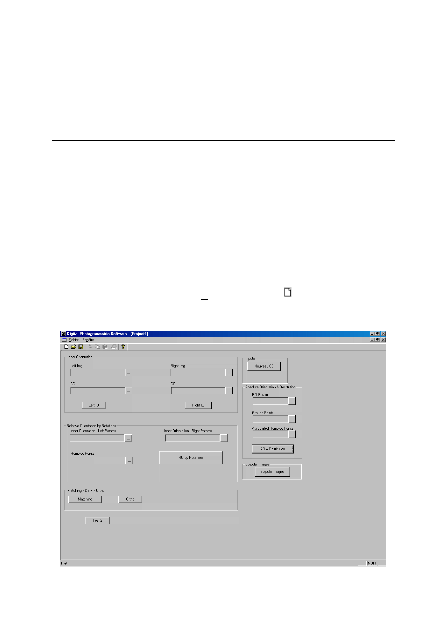
1. Create a project
Start
“Digital Photogrammetric Software“
On the File Menu, choose the option New Project or click
The project window will pop up:
26
2. Load the images
The program processes digital images with 8 bits/pixel (grey level). File format is
BMP.
The corresponding images for the Sart-Tilman are
- 1_7159.bmp for the left image
- 1_1760.bmp for the right image.
In the project window, click on the browser and choose 1_7159.bmp for the left
image and 1_7160.bmp for the right image.
3. Inner orientation
An inner orientation must be done for every image. This process allows establishing
a relation between the pixel and image coordinates. This relation is determined with
the help of the fiducial marks photo coordinates given in the calibration certificate
(see annex 1).
Encode the calibration certificate
In the project window, choose the option New CC. The following dialog box will pop
up:
27
y
x
The units of the calibration certificate are millimeters (10
-3
m). All the necessary data
are in the annex 1
When the entire certificate is encoded, save it. A CC file is created.
Location of fiducial marks
In the project window, choose the option Left and Right IO. The following window will
appear:
Below the images automatically appear the photo coordinates of the fiducial marks.
The first step is the determination of the photo orientation. According to it, the
parameters of transformation will change. In the example, the photo orientation is :
Then, you must track down the fiducial marks on the image.
28
Parameters of transformation will appear as from three fiducial marks and residues
as from four fiducial marks.
Correction of the radial lens distortion
In the menu Inner Orientation Module, choose the option Radial Distortion:
Then you can compute the coefficients of the polynomial after having chosen the
polynomial order. The values of the residues appear in the third column.
Before leaving the inner orientation, you must save the parameters:
menu Inner Orientation Module option Save OIparam. An OIParam File is created.
This operation must be done for the left and for the right image.
4. Relative orientation
Relative orientation allows determining the relative positions of the two bundles of
rays by creating spatial stereomodel in an arbitrary coordinate system. Tracking
down homologous points on the left and right images is necessary to make this
orientation.
Before starting the relative orientation, you must load the OIparam files of the left and
right images in the project window.
Click on the button RO by Rotations. The following window box will appear:
29
By clicking with the right mouse button on a grey case of the left inferior part of the
screen, you can choose to add a point with the option Add Point. Then you must
track down the homologous point on the left and right images:
The left and right image coordinates of the point will appear in the left inferior part of
the screen.
NB: It is possible to delete one point by clicking on the ID with the right mouse button
and by choosing the option Delete This Point.
As from five homologous points, RO Final Parameters (expressed in Radians) can be
computed by clicking on Reset the first time and after Iterate. Then values of the
chart will change: the parallax will decrease, new RO Final Parameters are computed
and new model coordinates (X
i
Coord, Y
i
Coord) are computed for every image. Stop
the iterations when you think that the parallax values are small enough and that RO
Final parameters don’t significantly change.
30
Before leaving the RO orientation, save the parameters by choosing the Save
Relative Orientation option in the Relative Orientation Module menu. An
ORparam File is created for every couple of images.
It is also possible to save the file with the image coordinates of the homologous
points by choosing the Save Hmlg File option in the Relative Orientation Module
menu. An hmlg File is created.
Another possibility is the loading of an already realised Hmlg File. Either you load
this file in the project dialog box before starting the RO by Rotations or you load the
file by choosing the option Load Hmlg File option in the Relative Orientation
Module menu.
5. Absolute orientation
The purpose of absolute orientation is the transformation from model coordinates to
ground coordinates. Control and check points are in the annex 2.
In the project window, click on AO & Restitution. There are two steps:
Determination of the parameters (menu Module option Determination)
As for the inner orientation, you can add or delete points by clicking on the right
mouse button. The following window will appear:
This window allows the encoding of the control, the check and the tie points. In the
point class, write ctrl for control points, check for checkpoints and tie for tie points
(statues of the points can be changed in the following steps).
Then you can track down these points on the two images. On the over view, control
points will appear in blue, checkpoints in green and tie points in red. As for three
control points, absolute orientation parameters can be computed by clicking on Reset
and then Iterate.
Stop the iterations when the residues on the control and checkpoints are small
enough.

31
To save the absolute orientation parameters:
menu Absolute Orientation Module option Save
– OA Params
A Oaparam file is created
To save the ground coordinates of the points:
menu Absolute Orientation Module option Save - Hmlg & Ground Points
An OA hmlg file is created, with the image coordinates of the homologous points
An OActrl file is created, with the ground coordinates of these points. Tie points will
not have ground coordinates. To have them, see the Restitution module
It is also possible to load files before realised:
menu Absolute Orientation Module option Load - Homolog Points to load the
image coordinates of the homologous points
menu Absolute Orientation Module option Load - Ground Points to load the
ground coordinates of the homologous points
Restitution (menu Module option Application)
This module allows to track down additional points for that ground coordinates are
unknown and to compute their ground coordinates with the absolute orientation
parameters. The ground coordinates of the new points will directly appear. These
points will receive the type resti points.
32
To save the ground coordinates of these new points:
menu Absolute Orientation Module option Save
– OAApply
An OAApply File is created
To load already tracked down points:
menu Absolute Orientation Module option Load OAApply
To make the eventual future realisation of plans easier, you can use the
geocodification module. This module allows generating files that can directly be
employed in topographic programs.
Create a Configuration File (.cl) that has the following structure
BEGIN_CODES
point
line
spline
END_CODES
BEGIN_LAYERS
road
hedge
fence
END_LAYERS
So you choose for every point its code and its layer. A file with the ID, the type, the
layer, the code and the coordinates of the points is created. This file can directly be
employed in topographic programs.
you put here all the layers that you want to use
you put here all the codes that you want to use
33
Automatic detection of homologous points (menu Configuration option AutoFind
– ON)
This module allows the automatic detection on the right image of the homologous
point tracked down on the left image. For the configuration of the correlation window,
refer to the points 3.5 and 3.6 of the data processing part.
6. Epipolar resampling
Epipolar images are images for that the
-parallaxes are removed.
The necessary inputs are:
- the original images (left and right)
- the calibration certificate
- the inner orientation parameters
In the project window, click on Epipolar Images. The following dialog box will pop up:
34
Load the necessary files in the corresponding cases.
Click on Compute Bounding Box to have the limits of this. These limits can be
changed. The X-limits depend on the overlay. The user can directly change the Y-
limits. To have more information about the determination of the limits, refer to point 4
of the data processing part.
When all these parameters are fixed, click on Process. You must directly give a
name and a File Path for the created image.
7. Image matching/DEM generation
In the project window, click on Matching
Image Matching
Image matching allows the automatic search of homologous points on the
overlapping area of several images. First choose the two images on which the
matching is made.
35
Click on Generate in the Matched Hmlg Points part. A dialog box allowing the
configuration of the matching will appear.

36
When you click on Configure Correlation Process, the same window that in the
automatic detection of homologous points (see the absolute orientation) will appear.
The superior part of the window contains various parameters. These are described
at the point 5 of the data processing part
For the predicted position of homologous points, there are two options:
Loading a homolog file
Computing an average shift X and Y values in pixels
When all these parameters are fixed, click on Process Matching. A window showing
the progress of the treatment appear. If you have made an error of configuration or if
the treatment is too long you have the possibility to stop it by clicking on Stop.
When the matching is finished, it is possible to visualize the matched points by
clicking Visualize.
ex: MatchEpi.hmlg
So you can delete eventual non-homologous points. It is also possible to load a file
with already matched points by clicking on Find and by choosing the adequate file.
DEM Generation
A DEM is a numeric representation of the heights of a surface. It is a regular grid of
points, localised with their planimetric coordinates, for that the heights were
interpolated as from known points.
For this step, you need a file containing ground coordinates. To have this file, either
load an already OAApply file by clicking on Find or generate a new file with
Generate. This new file is generated as from an hmlg file that must be load in the
Matched Hmlg Points case. The hmlg file can be constituted of homologous points
tracked down on the epipolar images
– then mark the Epipolar Img case – or of
homologous points tracked down on the original images.
For the epipolar images, you need the cc and OAparam files.
For the original images, you need the Left and Right OIparam, cc, ORparam and
OAparam files.
ex: ST.OAApply
When the OAApply file is loaded, you can click on Generate in the DEM part. The
DEM config window will appear:

37
Different parameters are proposed, that can be changed by the user. These are
described at the point 6 of the data processing part.
When the DEM is finished, save the file. A dem file is created.
ex: ST-5m.dem
8. Orthorectification
Orthorectification is the process of removing geometric errors inherent within
photography.
In the project window, click on Ortho.
38
To construct the orthophotograph, dem file, epipolar images, cc and OAparam files
must be loaded.
Predict parameters appear, that can be changed by the user. Click on Generate Left
Ortho and Generate Right Ortho. Save the images before leaving.
ex: ST_orthoG-0.5m.bmp
ST_orthoD-0.5m.bmp
It’s possible to have a view of the DEM draped with an orthophoto by activating the
option Generate VRML file. You can visualise this file with a VRML viewer available
on Internet.

39
ANNEXES

40
Annex 1
CALIBRATION
No.
AF/ZEISS JENA LMK 266632B/1
DATE
14. 3. 94
CAMERA CALIBRATION CERTIFICATE
LMK LENS CONE
No.
266632B
TYPE
ZEISS JENA LMK
41
CALIBRATION
No.
AF/ZEISS JENA LMK 266632B/1
DATE OF CALIBRATION
14.3.94
LENS TYPE:
ZEISS JENA LMK
Serial No
: 2666632B
FILTER TYPE
: NONE FITTED
ORIGIN OF MEASUREMENTS o:
The point of Symmetry
SIGN CONVENTION:
Distortion is positive if away from origin
CALIBRATED AT A TEMPERATURE OF 20°C
CALIBRATION PERFORMED BY:
D T PHILPOT
MEASUREMENTS
CALIBRATED PRINCIPAL DISTANCE:
152.314 mm
COORDINATES OF POINT OF SYMMETRY
x = -0.021
y = +0.003
COORDINATES OF PRINCIPAL POINT OF AUTOCOLLIMATION
x = -0.017
y = -0.003
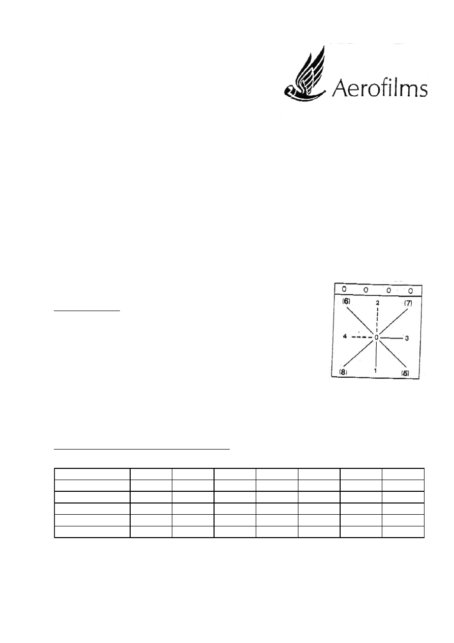
RADIAL DISTORTION IN MILLIMETRES
Back of camera
Radius (mm)
20
40
60
80
100
120
140
Semi diagonal (5)
0,003
0,004
0,003
0,001
0,000
-0,001
-0,005
Semi diagonal (6)
0,003
0,002
0,003
0,003
0,002
0,000
-0,002
Semi diagonal (7)
0,004
0,004
0,004
-0,001
0,000
-0,002
-0,006
Semi diagonal (8)
0,003
0,002
0,002
-0,001
0,002
0,004
-0,003
Mean
0,003
0,003
0,003
0,001
0,001
0,001
-0,004
42
CALIBRATION RESULTS FOR ZEISS RMK
CAMERA
ZEISS LMK 266632B
DATE
15 MARCH 1994
CENTRE OF GRAVITY
x = 110.0101
y = 109.9923
FIDUCIAL COORDINATES (SIDES)
x1 = 111.9978
x2 = -112.012
x3 = -0.01112
x4 = 0.009875
y1 = 0.020375
y2 = -0.00562
y3 = 111.9883
y4 = -111.998
DISTANCES
1-2 = 224.0100
3-4 = 223.9870
FIDUCIAL COORDINATES (CORNERS)
x5 = 109.9978
x6 = -109.992
x7 = -110.001
x8 = 110.0108
y5 = 110.0083
y6 = -110.007
y7 = 109.9843
y8 = -109.989
DISTANCES (DIAG)
7-8 = 311.1170
5-6 = 311.1312
DISTANCES (SIDE)
7-5 = 219.999
5-8 = 219.998
8-6 = 220.003
6-7 = 219.992
43
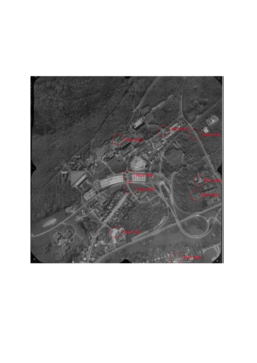
Annex 2
44
ROV001
– CTRL
middle of the sewage
X
Y
Z
234944.589
142672.707
242.564
ROV002
– CTRL
middle of the circular slab
X
Y
Z
234936.900
142094.695
232.874
ROV003
– CTRL
middle of the sewage
X
Y
Z
234566.378
142849.604
233.904
2
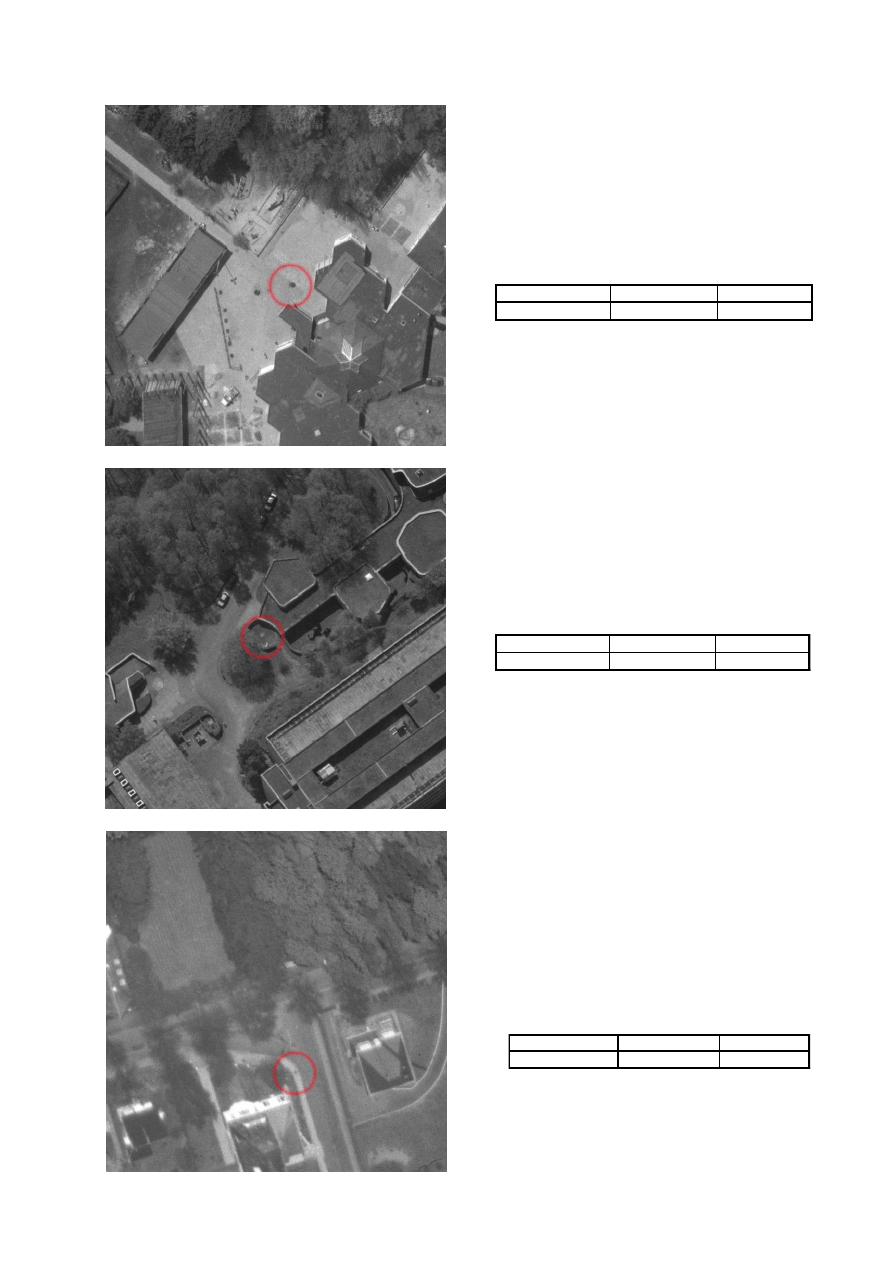
45
ROV004
– CTRL
extremity of the sewage
ROV005
– CTRL
middle of the sewage
X
Y
Z
234859.241
142401.975
246.506
ROV006
– CHECK
bottom of the parking banisters
X
Y
Z
234866.893
142323.762
244.944
X
Y
Z
234451.001
142059.345
245.169
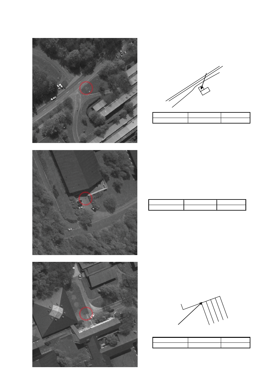
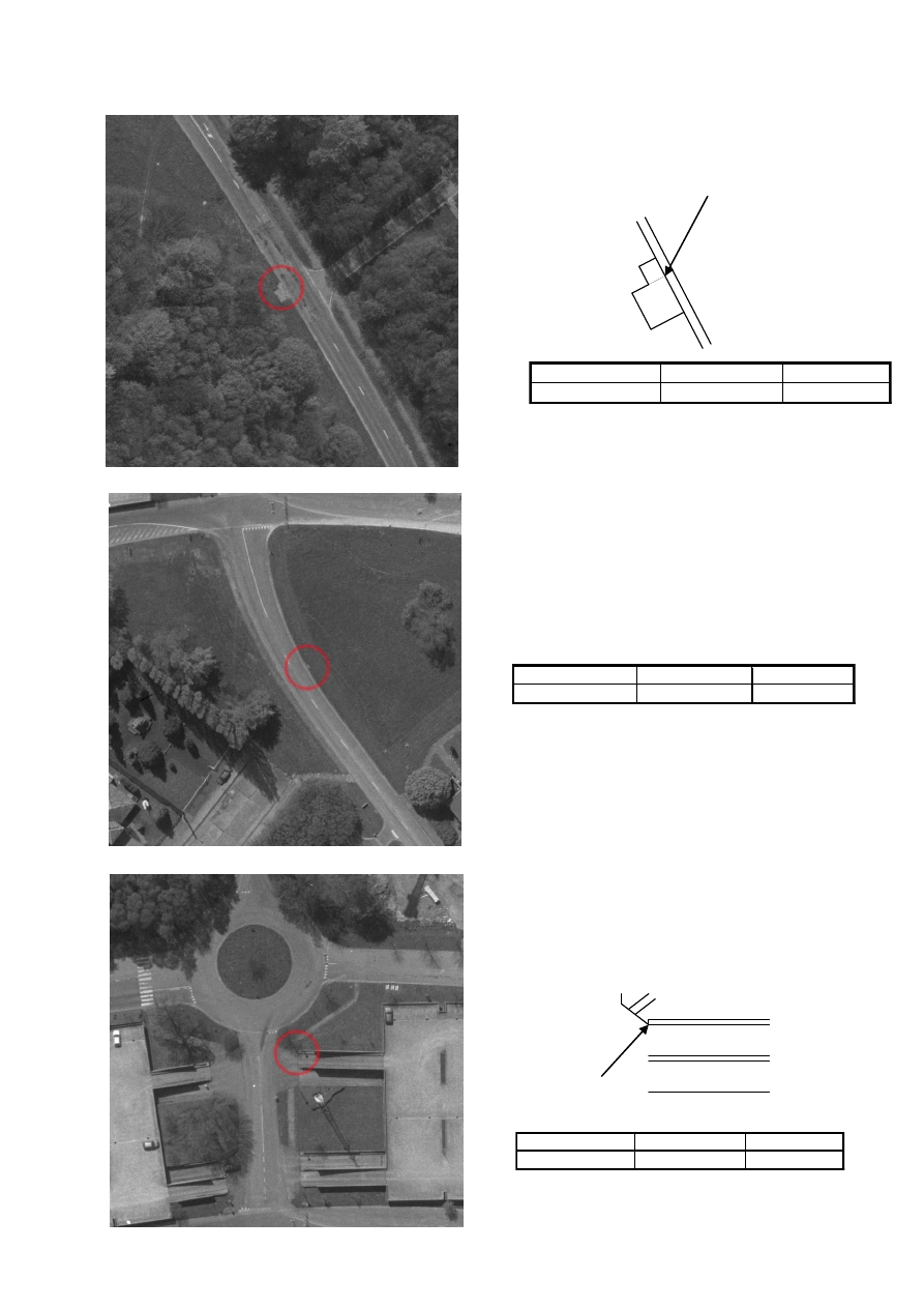
46
ROV008
– CHECK
middle of the sewage
X
Y
Z
234444.199
142440.695
241.045
ROV009
– CHECK
extremity of the stile
X
Y
Z
234422.382
142348.426
242.670
ROV007
– CHECK
middle of the sewage
X
Y
Z
234644.270
142036.037
241.687
Wyszukiwarka
Podobne podstrony:
M12 Oncore Users Guide Supplement
Mathcad Users Guide
Audio?ughter?rd Users Guide
Echo Link Users Guide
DFMProForNX Users Guide
MMConverter v2 0 Users Guide
PICkit 2 Users Guide
M12 Oncore Users Guide Supplement
Mathcad Users Guide
users guide PL
users guide
Faces 4 0 Users Guide
metasploit users guide
nikon d70 users guide
PBGrid Users Guide
PipBoxer V2 0 6 Users Guide
więcej podobnych podstron