MASSACHUSETTS INSTITUTE OF TECHNOLOGY

Department of Electrical Engineering

and Computer Science

Signals and Systems — 6.003

INTRODUCTION TO MATLAB — Fall 1999

Thomas F. Weiss

Last modification September 9, 1999

1

Contents

1 Introduction

3

2 Getting Started

3

3 Getting Help from Within MATLAB

4

4 MATLAB Variables — Scalars, Vectors, and Matrices

4

4.1

Complex number operations . . . . . . . . . . . . . . . . . . . . . . . . . . .

4

4.2

Generating vectors . . . . . . . . . . . . . . . . . . . . . . . . . . . . . . . .

5

4.3Accessing vector elements . . . . . . . . . . . . . . . . . . . . . . . . . . . .

5

5 Matrix Operations

5

5.1

Arithmetic matrix operations . . . . . . . . . . . . . . . . . . . . . . . . . .

6

5.2

Relational operations . . . . . . . . . . . . . . . . . . . . . . . . . . . . . . .

6

5.3Flow control operations . . . . . . . . . . . . . . . . . . . . . . . . . . . . . .

7

5.4

Math functions . . . . . . . . . . . . . . . . . . . . . . . . . . . . . . . . . .

7

6 MATLAB Files

7

6.1

M-Files

. . . . . . . . . . . . . . . . . . . . . . . . . . . . . . . . . . . . . .

8

6.1.1

Scripts . . . . . . . . . . . . . . . . . . . . . . . . . . . . . . . . . . .

8

6.1.2

Functions . . . . . . . . . . . . . . . . . . . . . . . . . . . . . . . . .

8

6.2

Mat-Files . . . . . . . . . . . . . . . . . . . . . . . . . . . . . . . . . . . . .

9

6.3Postscript Files . . . . . . . . . . . . . . . . . . . . . . . . . . . . . . . . . .

9

6.4

Diary Files . . . . . . . . . . . . . . . . . . . . . . . . . . . . . . . . . . . . .

10

7 Plotting

10

7.1

Simple plotting commands . . . . . . . . . . . . . . . . . . . . . . . . . . . .

11

7.2

Customization of plots . . . . . . . . . . . . . . . . . . . . . . . . . . . . . .

11

8 Signals and Systems Commands

11

8.1

Polynomials . . . . . . . . . . . . . . . . . . . . . . . . . . . . . . . . . . . .

11

8.2

Laplace and Z Transforms . . . . . . . . . . . . . . . . . . . . . . . . . . . .

12

8.3Frequency responses . . . . . . . . . . . . . . . . . . . . . . . . . . . . . . .

13

8.4

Fourier transforms and filtering . . . . . . . . . . . . . . . . . . . . . . . . .

13

9 Examples of Usage

13

9.1

Find pole-zero diagram, bode diagram, step response from system function .

13

9.1.1

Simple solution . . . . . . . . . . . . . . . . . . . . . . . . . . . . . .

14

9.1.2

Customized solution . . . . . . . . . . . . . . . . . . . . . . . . . . .

14

9.2

Locus of roots of a polynomial . . . . . . . . . . . . . . . . . . . . . . . . . .

16

9.3Response of an LTI system to an input . . . . . . . . . . . . . . . . . . . . .

18

10 Acknowledgement

18

2

1

Introduction

MATLAB is a programming language and data visualization software package which is es-
pecially effective in signal processing and systems analysis. This document is a brief in-
troduction to MATLAB that focuses on those features that are of particular importance in
6.003.

1

It is assumed that the reader is familiar with Project Athena, has an Athena account,

and has little or no experience with MATLAB. Other MATLAB help is available through
Athena consulting which offers a number of more tutorial handouts and short courses (ext.
3-4435), on-line consulting (type olc at the Athena prompt), and Athena on-line help (type
help at the Athena prompt). There are a number of books available that describe MAT-
LAB. For example, Engineering Problem Solving with Matlab, by D. M. Etter, published by
Prentice-Hall (1997) and Mastering MATLAB , by Hanselman and Littlefield, published by
Prentice-Hall (1996). The paperback MATLAB Primer by K. Sigmon, published by CRC
Press (1994) is a handy summary of MATLAB instructions. Further information about
MATLAB can be found at the web page of the vendor (The MathWorks, Inc.) whose URL
is http://www.mathworks.com. Full documentation can be purchased by contacting The
MathWorks.

2

Getting Started

On Project Athena, MATLAB can be accessed directly from the Dashboard (menu at the
top of the screen after you login to Project Athena) by using the hierarchical menu and
navigating as follows:

Numerical/Math//Analysis and Plotting//MATLAB.

MATLAB will then open a command window which contains the MATLAB prompt ‘>>’.

MATLAB contains a number of useful commands that are similar to UNIX commands,

e.g., ‘ls’, ‘pwd’, and ‘cd’. These are handy for listing MATLAB’s working directory, checking
the path to the working directory, and changing the working directory. MATLAB checks
for MATLAB files in certain directories which are controlled by the command ‘path’. The
command ‘path’ lists the directories in MATLAB’s search path. A new directory can be
appended or prepended to MATLAB’s search path with the command path(path,p) or
path(p,path) where p is some new directory, for example, containing functions written by
the user.

There is specially designed software available which can also be accessed from the Project

Athena Dashboard by navigating as follows:

Courseware//Electrical Engineering and Computer Science//

6.003 Signals and Systems//MATLAB.

These commands display a graphical user interface for exploring several important topics in
6.003. The same software is used in lecture demonstrations.

1

Revisions of this document will be posted on the 6.003 homepage on the web.

3

3

Getting Help from Within MATLAB

If you know the name of a function which you would like to learn how to use, use the ‘help’
command:

>>

help functionname

This command displays a description of the function and generally also includes a list of
related functions. If you cannot remember the name of the function, use the ‘lookfor’
command and the name of some keyword associated with the function:

>>

lookfor keyword

This command will display a list of functions that include the keyword in their descriptions.

Other help commands that you may find useful are ‘info’, ‘what’, and ‘which’. Descrip-

tions of these commands can be found by using the help command. MATLAB also contains
a variety of demos that can be with the ‘demo’ command.

4

MATLAB Variables — Scalars, Vectors, and Matri-
ces

MATLAB stores variables in the form of matrices which are M

× N, where M is the number

of rows and N the number of columns. A 1

× 1 matrix is a scalar; a 1 × N matrix is a row

vector, and M

×1 matrix is a column vector. All elements of a matrix can be real or complex

numbers;

√

−1 can be written as either ‘i’ or ‘j’ provided they are not redefined by the user.

A matrix is written with a square bracket ‘[]’ with spaces separating adjacent columns and
semicolons separating adjacent rows. For example, consider the following assignments of the
variable x

Real scalar

>> x = 5

Complex scalar

>> x = 5+10j (or >> x = 5+10i)

Row vector

>> x = [1 2 3] (or x = [1, 2, 3])

Column vector

>> x = [1; 2; 3]

3

× 3matrix

>> x = [1 2 3; 4 5 6; 7 8 9]

There are a few notes of caution. Complex elements of a matrix should not be typed with
spaces, i.e., ‘-1+2j’ is fine as a matrix element, ‘-1 + 2j’ is not. Also, ‘-1+2j’ is interpreted
correctly whereas ‘-1+j2’ is not (MATLAB interprets the ‘j2’ as the name of a variable.
You can always write ‘-1+j*2’.

4.1

Complex number operations

Some of the important operations on complex numbers are illustrated below

4

Complex scalar

>> x = 3+4j

Real part of x

>> real(x)

=

⇒ 3

Imaginary part of x

>> imag(x)

=

⇒ 4

Magnitude of x

>> abs(x)

=

⇒ 5

Angle of x

>> angle(x)

=

⇒ 0.9273

Complex conjugate of x

>> conj(x)

=

⇒ 3 - 4i

4.2

Generating vectors

Vectors can be generated using the ‘:’ command. For example, to generate a vector x that
takes on the values 0 to 10 in increments of 0.5, type the following which generates a 1

× 21

matrix

>>

x = [0:0.5:10];

Other ways to generate vectors include the commands: ‘linspace’ which generates a vector
by specifying the first and last number and the number of equally spaced entries between
the first and last number, and ‘logspace’ which is the same except that entries are spaced
logarithmically between the first and last entry.

4.3

Accessing vector elements

Elements of a matrix are accessed by specifying the row and column. For example, in the
matrix specified by A = [1 2 3; 4 5 6; 7 8 9], the element in the first row and third
column can be accessed by writing

>>

x = A(1,3) which yields 3

The entire second row can be accessed with

>>

y = A(2,:) which yields [4 5 6]

where the ‘:’ here means “take all the entries in the column”. A submatrix of A consisting
of rows 1 and 2 and all three columns is specified by

>>

z = A(1:2,1:3) which yields [1 2 3; 4 5 6]

5

Matrix Operations

MATLAB contains a number of arithmetic, relational, and logical operations on matrices.

5

5.1

Arithmetic matrix operations

The basic arithmetic operations on matrices (and of course scalars which are special cases
of matrices) are:

+

addition

-

subtraction

*

multiplication

/

right division

\

left division

^

exponentiation (power)

’

conjugate transpose

An error message occurs if the sizes of matrices are incompatible for the operation. Division
is defined as follows: The solution to A

∗ x = b is x = A\b and the solution to x ∗ A = b is

x = b/A provided A is invertible and all the matrices are compatible.

Addition and subtraction involve element-by-element arithmetic operations; matrix mul-

tiplication and division do not. However, MATLAB provides for element-by-element opera-
tions as well by prepending a ‘.’ before the operator as follows:

.*

multiplication

./

right division

.\

left division

.^

exponentiation (power)

.’

transpose (unconjugated)

The difference between matrix multiplication and element-by-element multiplication is

seen in the following example

>>A = [1 2; 3 4]
A =

1

2

3

4

>>B=A*A
B =

7

10

15

22

>>C=A.*A
C =

1

4

9

16

5.2

Relational operations

The following relational operations are defined:

6

<

less than

<=

less than or equal to

>

greater than

>=

greater than or equal to

==

equal to

~=

not equal to

These are element-be-element operations which return a matrix of ones (1 = true) and zeros
(0 = false). Be careful of the distinction between ‘=’ and ‘==’.

5.3

Flow control operations

MATLAB contains the usual set of flow control structures, e.g., for, while, and if, plus
the logical operators, e.g., & (and), | (or), and ~ (not).

5.4

Math functions

MATLAB comes with a large number of built-in functions that operate on matrices on an
element-by element basis. These include:

sin

sine

cos

cosine

tan

tangent

asin

inverse sine

acos

inverse cosine

atan

inverse tangent

exp

exponential

log

natural logarithm

log10

common logarithm

sqrt

square root

abs

absolute value

sign

signum

6

MATLAB Files

There are several types of MATLAB files including files that contain scripts of MATLAB
commands, files that define user-created MATLAB functions that act just like built-in MAT-
LAB functions, files that include numerical results or plots.

7

6.1

M-Files

MATLAB is an interpretive language, i.e., commands typed at the MATLAB prompt are
interpreted within the scope of the current MATLAB session. However, it is tedious to type
in long sequences of commands each time MATLAB is used to perform a task. There are two
means of extending MATLAB’s power — scripts and functions. Both make use of m-files
(named because they have a .m extension and they are therefore also called dot-m files)
created with a text editor like emacs. The advantage of m-files is that commands are saved
and can be easily modified without retyping the entire list of commands.

6.1.1

Scripts

MATLAB script files are sequences of commands typed with an editor and saved in an m-file.
To create an m-file using emacs, you can type from Athena prompt

athena%

emacs filename.m &

or from within MATLAB

>>

!

emacs filename.m &

Note that ‘!’ allows execution of UNIX commands directly. In the emacs editor, type
MATLAB commands in the order of execution. The instructions are executed by typing the
file name in the command window at the MATLAB prompt, i.e., the m-file filename.m is
executed by typing

>>

filename

Execution of the m-file is equivalent to typing the entire list of commands in the command
window at the MATLAB prompt. All the variables used in the m-file are placed in MAT-
LAB’s workspace. The workspace, which is empty when MATLAB is initiated, contains all
the variables defined in the MATLAB session.

6.1.2

Functions

A second type of m-file is a function file which is generated with an editor exactly as the
script file but it has the following general form:

function [output 1, output 2] = functionname(input1, input2)
%
%[output 1, output 2] = functionname(input1, input2) Functionname
%
% Some comments that explain what the function does go here.
%

8

MATLAB command 1;
MATLAB command 2;
MATLAB command 3;

The name of the m-file for this function is functionname.m and it is called from the MATLAB
command line or from another m-file by the following command

>>

[output1, output2] = functionname(input1, input2)

Note that any text after the ‘%’ is ignored by MATLAB and can be used for comments.
Output typing is suppressed by terminating a line with ‘;’, a line can be extended by typing
‘...’ at the end of the line and continuing the instructions to the next line.

6.2

Mat-Files

Mat-files (named because they have a .mat extension and they are therefore also called dot-
mat files) are compressed binary files used to store numerical results. These files can be
used to save results that have been generated by a sequence of MATLAB instructions. For
example, to save the values of the two variables, variable1 and variable2 in the file named
filename.mat, type

>>

save filename.mat variable1 variable2

Saving all the current variables in that file is achieved by typing

>>

save filename.mat

A mat-file can be loaded into MATLAB at some later time by typing

>>

load filename (or load filename.mat)

6.3

Postscript Files

Plots generated in MATLAB can be saved to a postscript file so that they can be printed at
a later time (for example, by the standard UNIX ‘lpr’ command). For example, to save the
current plot type

>>

print -dps filename.ps

The plot can also be printed directly from within MATLAB by typing

>>

print -Pprintername

9

0

1

2

3

4

5

6

7

8

-0.4

-0.3

-0.2

-0.1

0

0.1

0.2

0.3

0.4

Time (s)

Amplitude

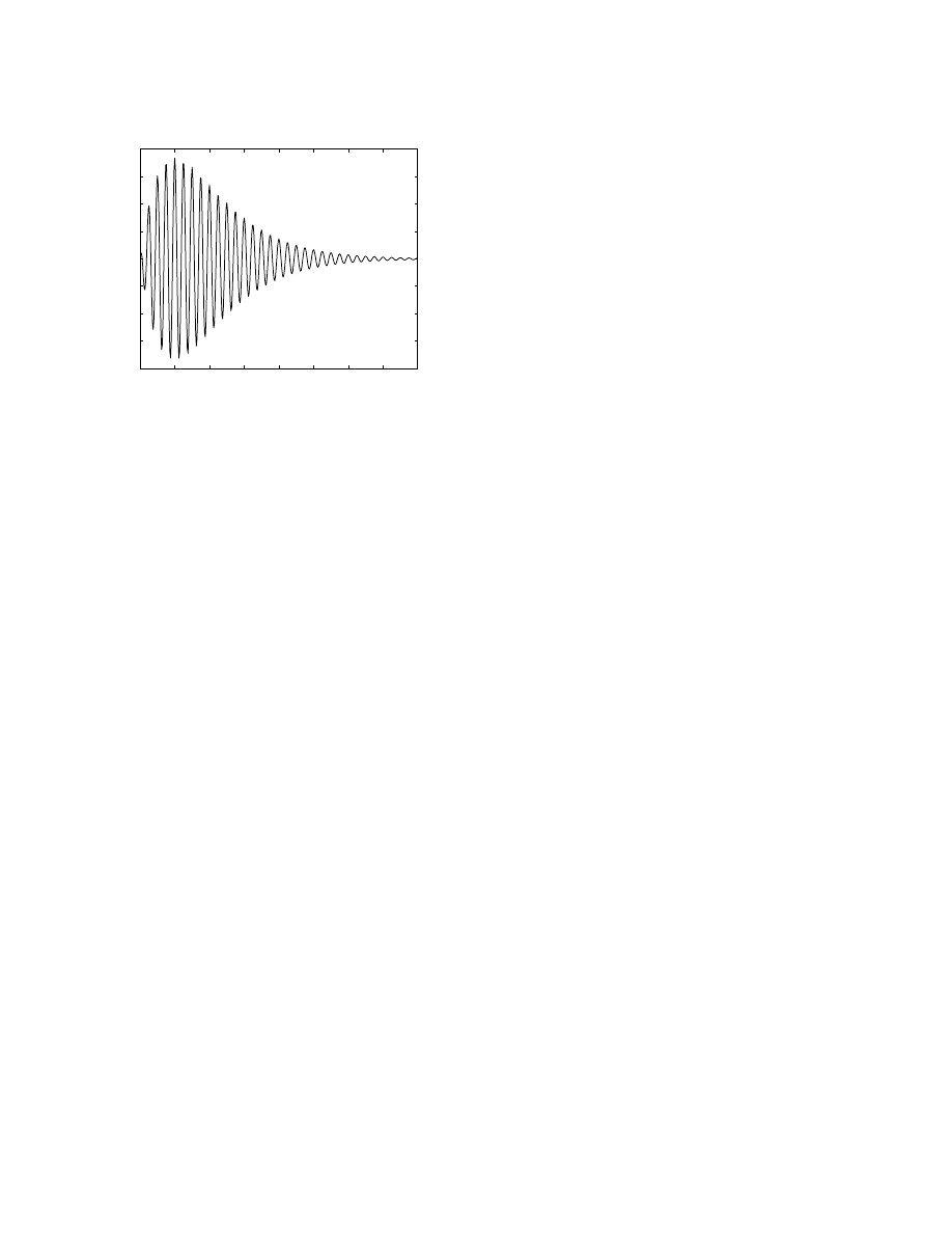
Figure 1: Example of the plotting of the
function x(t) = te

−t

cos(2π4t).

Type ‘help print’ to see additional options.

6.4

Diary Files

A written record of a MATLAB session can be kept with the diary command and saved
in a diary file. To start recording a diary file during a MATLAB session and to save it in
filename, type

>>

diary filename

To end the recording of information and to close the file type

>>

diary off

7

Plotting

MATLAB contains numerous commands for creating two- and three-dimensional plots. The
most basic of these commands is ‘plot’ which can have multiple optional arguments. A
simple example of this command is to plot a function of time.

t = linspace(0, 8, 401);

%Define a vector of times from ...

0 to 8 s with 401 points

x = t.*exp(-t).*cos(2*pi*4*t); %Define a vector of x values
plot(t,x);

%Plot x vs t

xlabel(’Time (s)’);

%Label time axis

ylabel(’Amplitude’);

%Label amplitude axis

This script yields the plot shown in Figure 1.

10

7.1

Simple plotting commands

The simple 2D plotting commands include

plot

Plot in linear coordinates as a continuous function

stem

Plot in linear coordinates as discrete samples

loglog

Logarithmic x and y axes

semilogx

Linear y and logarithmic x axes

semilogy

Linear x and logarithmic y axes

bar

Bar graph

errorbar

Error bar graph

hist

Histogram

polar

Polar coordinates

7.2

Customization of plots

There are many commands used to customize plots by annotations, titles, axes labels, etc.
A few of the most frequently used commands are

xlabel

Labels x-axis

ylabel

Labels y-axis

title

Puts a title on the plot

grid

Adds a grid to the plot

gtext

Allows positioning of text with the mouse

text

Allows placing text at specified coordinates of the plot

axis

Allows changing the x and y axes

figure

Create a figure for plotting

figure(n)

Make figure number n the current figure

hold on

Allows multiple plots to be superimposed on the same axes

hold off

Release hold on current plot

close(n)

Close figure number n

subplot(a,b,c)

Create an a

× b matrix of plots with c the current figure

orient

Specify orientation of a figure

8

Signals and Systems Commands

The following commands are organized by topics in signals and systems. Each of these
commands has a number of options that extend its usefulness.

8.1

Polynomials

Polynomials arise frequently in systems theory. MATLAB represents polynomials as row
vectors of polynomial coefficients. For example, the polynomial s

2

+ 4s

− 5 is represented in

11

MATLAB by the polynomial >> p = [1 4 -5]. The following is a list of the more impor-
tant commands for manipulating polynomials.

roots(p)

Express the roots of polynomial p as a column vector

polyval(p,x)

Evaluate the polynomial p at the values contained in the vector x

conv(p1,p2)

Computer the product of the polynomials p1 and p2

deconv(p1,p2)

Compute the quotient of p1 divided by p2

poly2str(p,’s’)

Display the polynomial as an equation in s

poly(r)

Compute the polynomial given a column vector of roots r

8.2

Laplace and Z Transforms

Laplace transforms are an important tool for analysis of continuous time dynamic systems,
and Z transforms are an important tool for analysis of discrete time dynamic systems. Im-
portant commands to manipulate these transforms are included in the following list.

residue(n,d)

Compute the partial fraction expansion of the ratio of polynomials
n(s)/d(s)

lsim(SYS,u)

Compute/plot the time response of SYS to the input vector u

step(SYS)

Compute/plot the step response of SYS

impulse(SYS)

Compute/plot the impulse response of SYS

pzmap(n,d)

Compute/plot a pole-zero diagram of SYS

residuez(n,d)

Compute the partial fraction expansion of the ratio of polynomials
n(z)/d(z) written as functions of z

−1

rlocus(SYS)

Compute/plot the root locus for a system whose open loop system is
specified by SYS

dlsim(n,d,u)

Compute the time response to the input vector u of the system with
system function n(z)/d(z)

dstep(n,d)

Compute the step response of the system with system function
n(z)/d(z)

dimpulse(n,d)

Compute the impulse response of the system with system function
n(z)/d(z)

zplane(z,p)

Plot a pole-zero diagram from vectors of poles and zeros, p and z

A number of these commands work with several specifications of the LTI system. One
such specification is in terms of the transfer function for which ‘SYS’ is replaced with
‘TF(num,den)’ where ‘num’ and ‘den’ are the vectors of coefficients of the numerator and
denominator polynomials of the system function.

12

8.3

Frequency responses

There are several commands helpful for calculating and plotting frequency response given
the system function for continuous or discrete time systems as ratios of polynomials.

bode(n,d)

Plot the Bode diagram for a CT system whose system function is a the
ratio of polynomials n(s)/d(s)

freqs(n,d)

Compute the frequency response for a CT system with system function
n(s)/d(s)

freqz(n,d)

Compute the frequency response for a DT system with system function
n(z)/d(z)

8.4

Fourier transforms and filtering

There is a rich collection of commands related to filtering. A few basic commands are listed
here.

fft(x)

Compute the discrete Fourier transform of the vector x

ifft(x)

Compute the inverse discrete Fourier transform of the vector x

fftshift

Shifts the fft output from the discrete range frequency range (0, 2π) to
(

−π, π) radians

filter(n,d,x)

Filters the vector x with a filter whose system function is n(z)/d(z),
includes some output delay

filtfilt(n,d,x)

Same as filter except without the output delay

In addition there are a number of filter design functions including firls, firl1, firl2,
invfreqs, invfreqz, remez, and butter. There are also a number of windowing functions
including boxcar, hanning, hamming, bartlett, blackman, kaiser, and chebwin.

9

Examples of Usage

9.1

Find pole-zero diagram, bode diagram, step response from
system function

Given a system function

H(s) =

s

s

2

+ 2s + 101

,

MATLAB allows us to obtain plots of the pole-zero diagram, the Bode diagram, and the
step response.

13

-1

-0.9

-0.8

-0.7

-0.6

-0.5

-0.4

-0.3

-0.2

-0.1

0

-10

-8

-6

-4

-2

0

2

4

6

8

10

Real Axis

Imag Axis

10

-1

10

0

10

1

10

2

-80

-60

-40

-20

0

Frequency (rad/sec)

Gain dB

10

-1

10

0

10

1

10

2

-90

0

90

Frequency (rad/sec)

Phase deg

0

0.5

1

1.5

2

2.5

3

3.5

4

4.5

5

-0.08

-0.06

-0.04

-0.02

0

0.02

0.04

0.06

0.08

0.1

Time (secs)

Amplitude

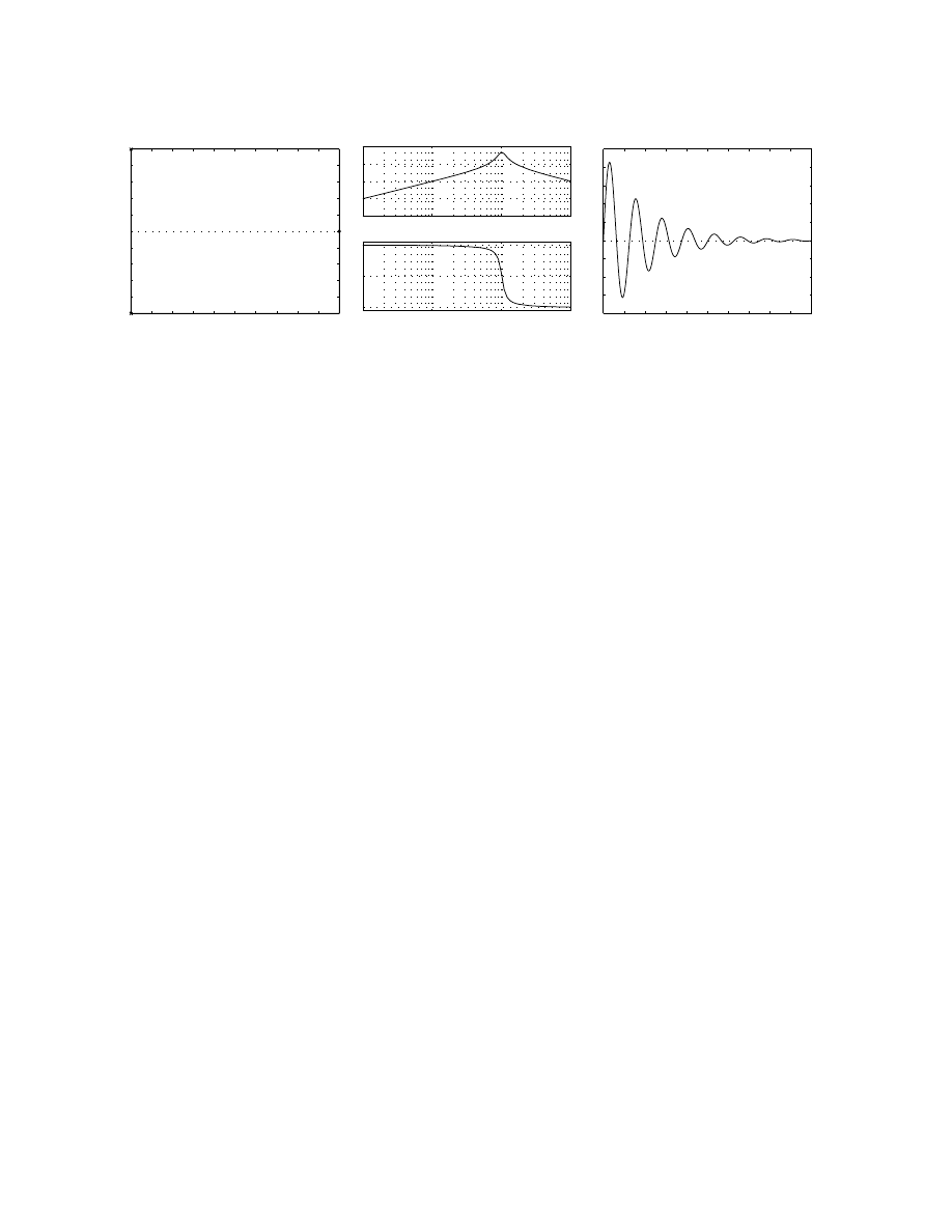
Figure 2: The plots were generated by the script and each plot was saved as an encapsulated
postscript file. The three files were scaled by 0.3and included in the document.

9.1.1

Simple solution

The simplest way to obtain the requisite plots is to let MATLAB choose all the scales, labels,
and annotations with the following script.

num = [1 0];

%Define numerator polynomial

den = [1 2 101];

%Define denominator polynomial

%% Pole-zero diagram
figure(1)

%Create figure 1

pzmap(num,den);

%Plot pole-zero diagram in figure 1

%% Bode diagram
figure(2);

%Create figure 2

bode(num,den);

%Plot the Bode diagram in figure 2

%% Step response
figure(3);

%Create figure 3

step(num,den);

%Plot the step response in figure 3

This script leads to the individual plots shown in Figure 2.

9.1.2

Customized solution

It may be desirable to display the results with more control over the appearance of the plot.
The following script plots the same results but shows how to add labels, add titles, define
axes scales, etc.

%% Define variables
t = linspace(0,5,201);

%Define a time vector with 201 ...

equally-spaced points from 0 to 5 s.

w = logspace(-1,3,201);

%Define a radian frequency vector ...

with 201 logarithmically-spaced ...

14

points from 10^-1 to 10^3 rad/s

num = [1 0];

%Define numerator polynomial

den = [1 2 101];

%Define denominator polynomial

[poles,zeros] = pzmap(num,den); %Define poles to be a vector of the ...

poles and zeros to be a vector of ...
zeros of the system function

[mag,angle] = bode(num,den,w);

%Define mag and angle to be the ...

magnitude and angle of the ...
frequency response at w

[y,x] = step(num,den,t);

%Define y to be the step response ...

of the system function at t

%% Pole-zero diagram
figure(1)

%Create figure 1

subplot(2,2,1)

%Define figure 1 to be a 2 X 2 matrix ...

of plots and the next plot is at ...
position (1,1)

plot(real(poles),imag(poles),’x’,real(zeros),imag(zeros),’o’); %Plot ...

pole-zero diagram with x for poles ...
and o for zeros

title(’Pole-Zero Diagram’);

%Add title to plot

xlabel(’Real’);

%Label x axis

ylabel(’Imaginary’);

%Label y axis

axis([-1.1 0.1 -12 12]);

%Define axis for x and y

grid;

%Add a grid

%% Bode diagram magnitude
subplot(2, 2, 2);

%Next plot goes in position (1,2)

semilogx(w,20*log10(mag));

%Plot magnitude logarithmically in w ...

and in decibels in magnitude

title(’Magnitude of Bode Diagram’);
ylabel(’Magnitude (dB)’);
xlabel(’Radian Frequency (rad/s)’);
axis([0.1 1000 -60 0]);
grid;
subplot(2, 2, 4);

%Next plot goes in position (2,2)

semilogx(w,angle);

%Plot angle logarithmically in w and ...

linearly in angle

title(’Angle of Bode Diagram’);
ylabel(’Angle (deg)’);
xlabel(’Radian Frequency (rad/s)’);
axis([0.1 1000 -90 90]);
grid;

15

-1

-0.5

0

-10

-5

0

5

10

Pole-Zero Diagram

Real

Imaginary

10

0

10

2

-60

-40

-20

0

Magnitude of Bode Diagram

Magnitude (dB)

Radian Frequency (rad/s)

10

0

10

2

-50

0

50

Angle of Bode Diagram

Angle (deg)

Radian Frequency (rad/s)

0

2

4

6

-0.1

-0.05

0

0.05

0.1

Step Response

Time (s)

Amplitude

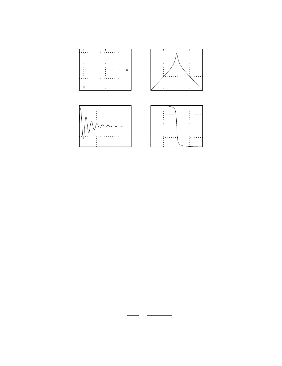
Figure 3: This combined plot was generated by the script and saved as an encapsulated
postscript file which was scaled by 0.6 and included in the document.

%% Step Response

%Next plot goes in position (2,1)

subplot(2, 2, 3);
plot(t,y);

%Plot step response linearly in t and y

title(’Step Response’);
xlabel(’Time (s)’);
ylabel(’Amplitude’);
grid;

This script leads to the plot shown in Figure 3.

9.2

Locus of roots of a polynomial

In analyzing a system, it is often of interest to determine the locus of the roots of a polynomial
as some parameter is changed. A common example is to track the poles of a closed-loop
feedback system as the open loop gain is changed. For example, in the system shown in
Figure 4, the closed loop gain is given by Black’s formula as

H(s) =

Y (s)

X(s)

=

G(s)

1 + KG(s)

.

If G(s) is a rational function in s then it can be expressed as

16

+

+

−

X(s)

Y (s)

G (s)

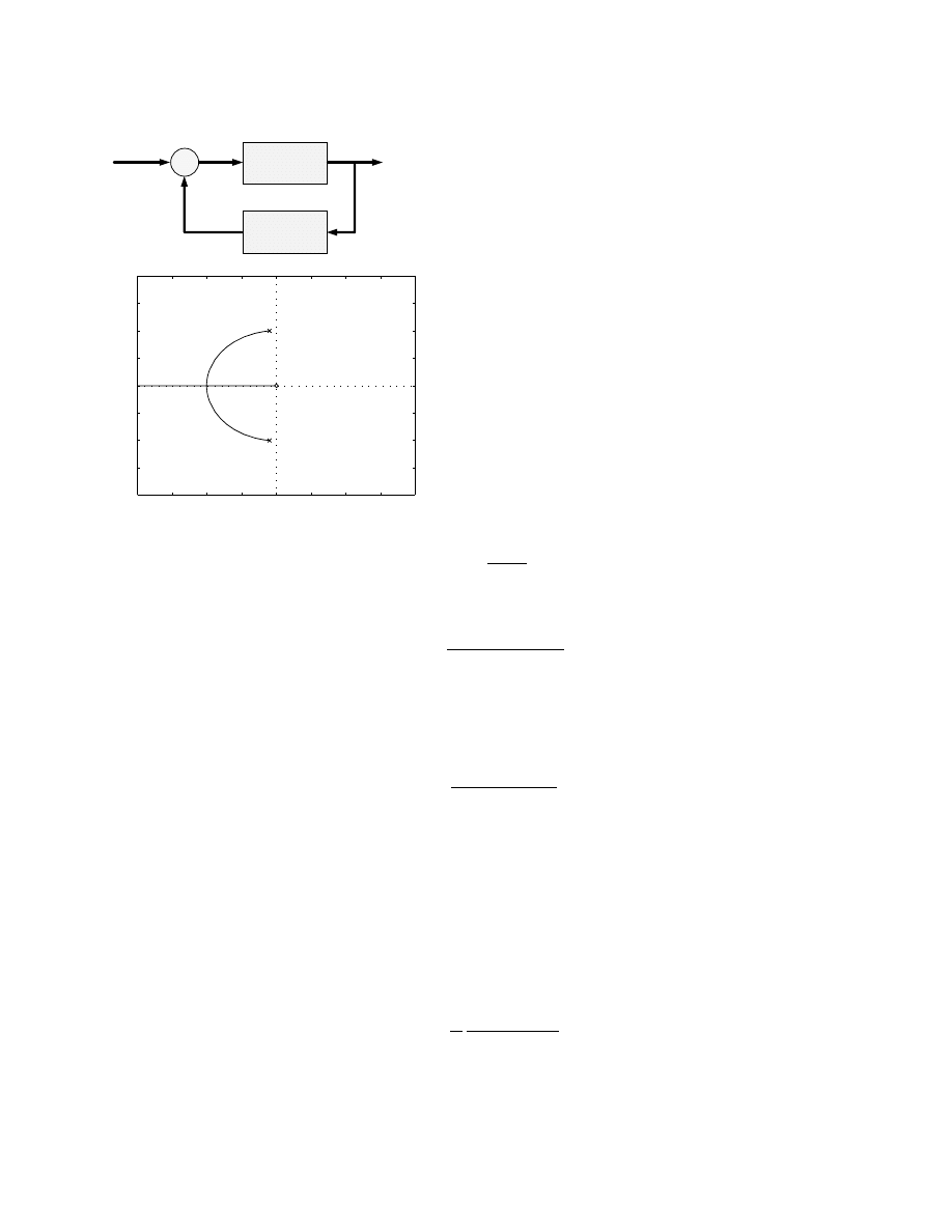
K

Figure 4: Feedback system with open loop gain
G(s).

-20

-15

-10

-5

0

5

10

15

20

-20

-15

-10

-5

0

5

10

15

20

Real Axis

Imag Axis

Figure 5: Root-locus plot of the poles of H(s)
as K varies for G(s) = s/(s

2

+ 2s + 101).

G(s) =

N (s)

D(s)

where N (s) and D(s) are polynomials. Solving for H(s) yields

H(s) =

N (s)

D(s) + KN (s)

.

Finding the poles of H(s) as K changes implies finding the roots of the polynomial D(s) +
KN (s) as K changes. Because this is such a common computation, MATLAB provides a
function for computing the root locus conveniently called ‘rlocus’. The following script
plots the root locus for G(s)

G(s) =

s

s

2

+ 2s + 101

.

num = [1 0];

%Define numerator polynomial

den = [1 2 101];

%Define denominator polynomial

figure(1);
rlocus(num,den)

%Plot root locus

The plot is shown in Figure 5. The root-locus plot can be customized in a manner similar
to the example given above, see ‘help rlocus’.

The command rlocus can be used in other contexts. For example, suppose we have a

series R, L, C circuit whose admittance is

Y (s) =

1

L

s

s

2

+ Rs + 2

,

and we wish to obtain a plot of the locus of the poles (roots of the denominator polynomial)
as the resistance R varies. It is only necessary to parse the denominator polynomial into two
parts N (s) = s and D(s) = s

2

+ 2 and use ‘rlocus’ to obtain the plot.

17

0

1

2

3

4

5

6

7

8

9

10

-1

-0.8

-0.6

-0.4

-0.2

0

0.2

0.4

0.6

0.8

1

Time (s)

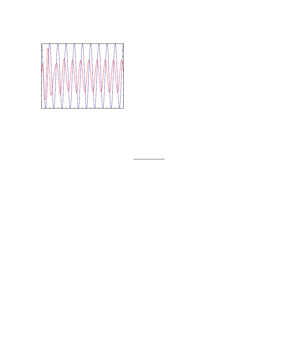
Amplitude

Figure 6: The input time function is a cos-
inusoid that starts at t = 0.

The out-

put of an LTI system with system function
H(s) = 5s/(s

2

+ 2s + 101) is shown in red.

9.3

Response of an LTI system to an input

The MATLAB command lsim makes it easy to compute the response of an LTI system with
system function H(s) to an input x(t). Suppose

H(s) =

5s

s

2

+ 2s + 101

,

and we wish to find the response to the input x(t) = cos(2πt) u(t). The following script
computes and plots the response.

figure(1);
num = [5 0];

%Define numerator polynomial

den = [1 2 101];

%Define denominator polynomial

t = linspace(0, 10, 401);

%Define a time vector

u = cos(2*pi*t);

%Compute the cosine input function

[y,x] = lsim(num,den,u,t); %Compute the response to the input u at times t
plot(t,y,’r’,t,u,’b’);

%Plot the output in red and the input in blue

xlabel(’Time (s)’);
ylabel(’Amplitude’);

The plot is shown in Figure 6.

10

Acknowledgement

This document makes use of earlier documents prepared by Deron Jackson and by Alan
Gale.

18