
The Arrow of Time
in
Cosmology and Statistical Physics
SEBASTIAAN KOLE
Eerste referent: Dr G.J.Stavenga
Co-referent: Prof.dr D.Atkinson
Derde beoordelaar: Prof.dr T.A.F.Kuipers
Faculteit der Wijsbegeerte
Rijksuniversiteit Groningen
Datum goedkeuring: juli 1999


Contents
I Chaos out of order
9
1 The Second Law
11
1.1 Introduction . . . . . . . . . . . . . . . . . . . . . . . . . . . . . . . . . . . . . 11
1.2 Thermodynamical entropy . . . . . . . . . . . . . . . . . . . . . . . . . . . . . . 12
1.3 The
H
-theorem . . . . . . . . . . . . . . . . . . . . . . . . . . . . . . . . . . . 13
1.4 The rise of statistical mechanics . . . . . . . . . . . . . . . . . . . . . . . . . . 15
1.5 Non-equilibrium phenomena . . . . . . . . . . . . . . . . . . . . . . . . . . . . . 17
1.5.1 The ensemble formalism . . . . . . . . . . . . . . . . . . . . . . . . . . 18
1.5.2 The approach to equilibrium . . . . . . . . . . . . . . . . . . . . . . . . 19
2 Time Asymmetry and the Second Law
23
2.1 Introduction . . . . . . . . . . . . . . . . . . . . . . . . . . . . . . . . . . . . . 23
2.2 Interventionism . . . . . . . . . . . . . . . . . . . . . . . . . . . . . . . . . . . 25
2.3 Initial conditions . . . . . . . . . . . . . . . . . . . . . . . . . . . . . . . . . . . 26
2.3.1 Krylov and the preparation of a system . . . . . . . . . . . . . . . . . . . 26
2.3.2 Prigogine and singular ensembles . . . . . . . . . . . . . . . . . . . . . . 26
2.4 Branch systems . . . . . . . . . . . . . . . . . . . . . . . . . . . . . . . . . . . 27
2.4.1 Reichenbach's lattice of mixture . . . . . . . . . . . . . . . . . . . . . . 28
2.4.2 Davies' non-existing prior states . . . . . . . . . . . . . . . . . . . . . . 28
2.5 Conclusion . . . . . . . . . . . . . . . . . . . . . . . . . . . . . . . . . . . . . . 29
3 Contemporary discussions
31
3.1 Introduction . . . . . . . . . . . . . . . . . . . . . . . . . . . . . . . . . . . . . 31
3.2 Cosmology and information theory . . . . . . . . . . . . . . . . . . . . . . . . . 31
3.3 A unied vision of time . . . . . . . . . . . . . . . . . . . . . . . . . . . . . . . 33
3.4 The atemporal viewpoint . . . . . . . . . . . . . . . . . . . . . . . . . . . . . . 34
3.5 Conclusion . . . . . . . . . . . . . . . . . . . . . . . . . . . . . . . . . . . . . . 35
II The emergence of time
37
4 Introduction
39

4
Contents
5 In the Beginning
43
5.1 The Big Bang . . . . . . . . . . . . . . . . . . . . . . . . . . . . . . . . . . . . 44
5.2 Initial conditions and ination . . . . . . . . . . . . . . . . . . . . . . . . . . . . 46
5.3 Another way out? . . . . . . . . . . . . . . . . . . . . . . . . . . . . . . . . . . 49
6 In the End
51
6.1 Quantum cosmology . . . . . . . . . . . . . . . . . . . . . . . . . . . . . . . . . 52
6.2 Time symmetric cosmologies . . . . . . . . . . . . . . . . . . . . . . . . . . . . 53
6.3 Conclusions . . . . . . . . . . . . . . . . . . . . . . . . . . . . . . . . . . . . . 57
7 Review and main conclusions
59
7.1 The Second Law . . . . . . . . . . . . . . . . . . . . . . . . . . . . . . . . . . . 59
7.2 Cosmology . . . . . . . . . . . . . . . . . . . . . . . . . . . . . . . . . . . . . . 60
7.3 Main Conclusions . . . . . . . . . . . . . . . . . . . . . . . . . . . . . . . . . . 62
Glossary of technical terms
63
References
67

Introduction
A subject of both a philosophical and a physical nature is the arrow of time. Many people are not
aware of the problem of the arrow of time and wonder why there should be a problem since there
is nothing more natural than the ow of time. In this report I will show that there are indeed
problems concerning the arrow of time. The arrow of time could be described as the direction of
time in which a particular process naturally occurs. If one would record such a process (say on
video), play it backwards and conclude there is something strange happening then that process
occurred in one specic direction of time. People for example remember the past and can only
imagine (or predict) the future. Does this x the arrow of time? We will see that this is only a
manifestation of one particular arrow of time: the psychological arrow of time. It could simply
be dened as the direction of time which people experience.
There are several other arrows of time. Each of these arrows describes a process or class of
processes always evolving in the same direction of time. The direction of time in which chaos
increases denes the thermodynamical arrow time. If one accidentally drops a plate on the ground,
then it breaks and the scattered pieces will not join each other by themselves (unless one records
his clumsiness and plays it backwards). The same point can be made if one throws a rock in a
pond. As it enters the water, waves start diverging and gradually damp out. The reverse event,
where waves start converging and a rock is thrown out of the pond is never observed. This process
constitutes the arrow of time of radiation. On the grand scale of the entire universe a similar
process is known: the overall expansion of the universe. The direction of time in which the size
of the universe increases is called the cosmological arrow of time. Other arrows can be identied
but they will play no important role in this report.
The arrows mentioned are not completely independent of each other. I will show in detail
how specic arrows are related to other arrows, but for now we can take the following picture for
granted: the psychological arrow is dened by the thermodynamical arrow, which depends on the
radiative arrow (although some people argue otherwise), which in its turn is ultimately grounded
in the cosmological arrow.
The arrows of time could be denoted as phenomenological facts of nature. They describe time
asymmetrical processes, processes which behave dierently in one direction of time with respect
to the other direction. The main problem that arises now is that the major laws of physics are
time symmetrical. To get some feeling for what exactly time symmetry for physical laws entails,
I will state three possible denitions (as pointed out by Savitt in [42, pp. 12{14]):
Denition 1.
A physical theory is time reversal invariant if every solution of the dierential
equations (provided the theory can be expressed in dierential equations, but this is generally
the case) still satises the dierential equations under time reversal of the solution:
t
replaced by
;t
.
Denition 2.
Denote the evolution of the system as a sequence of states:
S
i
time
;
!
S
f
. A
6
Introduction
sequence of states is dynamically possible if it is consistent with the theory. Now, a physical
theory is time reversal invariant if such a sequence of states is dynamically possible if and
only if the sequence
(S
f
)
R
time
;
!
(S
i
)
R
is dynamically possible, where
(S
)
R
denotes the time
reversed equivalent of the state
S
(e.g. a system with the spins and velocities of all its
particles reversed). It thus places extra constraints on a sequence of states, compared with
denition 1.
Denition 3.
A physical theory is time reversal invariant if and only if should
S
i
evolve to
S
f
then
(S
f
)
R
must evolve to
(S
i
)
R
. This denition is stronger than denition 2 in the sense
that a theory allowing a system to contain a bifurcation point
1
would not be time reversal
invariant according to this denition.
How then can physics explain time asymmetrical phenomena within a time symmetrical frame-
work? This will be the central question of this report and I will focus on two particular arrows of
time in answering it: the thermodynamical and cosmological arrows of time. But, rst of all, we
should be suspicious of what reasoning can be accepted as a `good' explanation and what cannot.
Many people `solve' the problem of deriving an asymmetrical arrow of time from time sym-
metric laws by applying a double standard: they accept certain assertions about one direction of
time which they would not accept in the opposite direction. The time asymmetry is thus explicitly
inserted without sound arguments. The principle fallaciously used in such a way is called PI
3
by
Price [37]: the principle of independence of incoming inuences, which tells us that systems are
independent of one another before they interact. When used without a similar principle concerning
the independence of systems after they have interacted, this principle is clearly time asymmetrical.
Closely connected to the double standard fallacy is what Sklar [21] calls the `parity of reasoning
problem'. Any reasoning which is in itself time symmetrical and which is invoked to explain a time
asymmetrical phenomenon can similarly be applied to project the behavior of such a phenomenon
backwards in time and predict possibly a counter factual process. Somewhere in the derivation of
a time asymmetrical theory, an asymmetrical principle or law will have to be used to escape this
parity of reasoning.
Now we can understand why a theory explaining the asymmetry of the Second Law has its
limitations [37, pag. 44]. The main issue is that such a theory either has to be time symmetrical
and consequently fails to explain the asymmetry or it has to treat the two directions of time
dierently and fallaciously applies a double standard concerning the two directions of time. This
can be demonstrated as follows: A theory predicting the dynamical evolution of a system, from
time equals
t
to
t
+
dt
, must give a symmetrical result when the information whether
dt
is positive
or negative is missing since it has to treat the two cases dierently right from the beginning in
order to reach asymmetry. The only way to escape this limitation is to use an objective direction
of time as reference, but the existence of such a reference can be doubted. Stating that the
direction of time is the direction in which entropy increases would be a petitio principii.
Penrose [33] actually suggested to impose the time asymmetry explicitly by his `principle of
causality': `A system which has been isolated throughout the past is uncorrelated with the rest
of the universe.' We shall see in the next chapter that this principle is very similar to an Ansatz
Boltzmann made to derive his time asymmetrical
H
-theorem. To summarize: the use of any time
asymmetrical principle must be justied because of the crucial role it plays in deriving a time
asymmetric theory.
1
A bifurcation point is a concept from chaos theory which occurs when a system is allowed to `choose' among
a set of dierent future evolutions. The actual choice cannot be known beforehand. A bifurcation point applies to
both directions of time since it is only dependent upon the state prior to the bifurcation.

Introduction
7
Outline
In the rst part of this report the thermodynamical arrow of time will be investigated. The explicit
direction of time that can be observed in any thermodynamical system is commonly known as
the Second Law of Thermodynamics. Now, the derivation of this law from rst principles poses
a serious problem for physicists. First principles are for example Newtonian mechanics, which
are time symmetric. Somewhere along the line in the derivation of the Second Law a time
asymmetrical principle has to be put into the theory, and an arrow of time is thus explicitly
inserted. I will try to pin down where in each theory this occurs.
The main line I will follow in my discussion of the subject is of a historical nature. The
development of the theory of statistical mechanics and the subsequent problems, considering its
foundation, quite naturally allow an investigation into the foundation of the arrow of time of the
Second Law. Following the historical development, various concepts will be introduced providing
the necessary context of contemporary discussions on the subject. As the theories are being
discussed, I will analyze their shortcomings and inconsistencies in justifying the introduction of
time-asymmetrical principles. A `good' theory explaining the time-asymmetrical character of the
Second Law should be, in my opinion, ultimately grounded in `facts' nobody doubts. One can
think of the fundamental laws of physics and boundary conditions of the early universe. I will
investigate whether a derivation starting from these facts is possible, and see which problems are
encountered in an attempt to do so. How the ultimate boundary conditions of the universe may
be explained is a matter to which we will return in the second part of this thesis.
To continue with the outline of the rst part, after a short introduction to thermodynamical
entropy in the beginning of Chapter 1, I will look at the rst attempt, made by Boltzmann, to
ground the irreversible character of the Second Law. This is precisely what he established with
his so-called
H
-theorem. His contemporaries immediately raised two objections: the reversibility
and recurrence objections. In response, he developed a statistical viewpoint in which there was
essentially no place for irreversibility. He sought the nal explanation of temporal asymmetry in
cosmological uctuations. Another approach to ground thermodynamics was made by Gibbs. He
developed the so-called ensemble formalism. This formalism is statistical in nature and immune
from the recurrence objection. The very denition of entropy, however, is essential, and one of the
main problems is that one particular denition, viz. that of ne-grained entropy, remains constant
in time. However, the time asymmetrical entropy increase might be established using another,
more `subjective', denition of entropy: that of coarse-grained entropy. The actual increase of
this coarse-grained entropy remains a problematic issue. Using very general arguments, one can
show that coarse-grained entropy increases (if the system is initially not in a state of equilibrium)
but the time involved and the monotonicity of the approach to equilibrium remain unclear. More
rigorous attempts to explain the actual approach to equilibrium will be examined in Chapter 1 but
they will all turn out to rely in some way on assumptions comparable to the assumption Boltzmann
made when he derived his
H
-theorem, viz. the assumption of molecular chaos. If these so-called
rerandomization posits are not taken to be time asymmetric in themselves, and the possibility
that a system might not be totally isolated remains unexploited, then the ultimate source of time
asymmetry is by most people sought in the particular initial conditions of the system. Various
attempts to explain why of all the possible initial conditions only those occur that lead to entropy
increase, will be examined in Chapter 2. In Chapter 3, I will review alternative approaches to
establish the time asymmetry of the Second Law, followed by some concluding remarks.
The outline of the part about the arrow of time in cosmology will be mainly given in the rst

8
Introduction
chapter constituting that part. We will delve into the mysteries of the early universe, the Big
Bang, as well as its ultimate end, the Big Crunch (in the case that it will occur) and the path
the universe will follow towards this end. Along the way many abstract and exotic concepts, such
as black holes, grand unied theories and the wave function of the universe, will be part of the
discussion. The central questions will be how to explain the low entropy of the universe and the
alignment of the various arrows of time throughout every phase of the universe. In doing this,
the connection between the arrows of time will be claried.
In the nal chapter an overview will be given and the main conclusions will be restated.

P
a
rt
I
Chaos out of order


Chapter
1
The Second Law
\We have looked through the window on the world provided by the Second law, and have
seen the naked purposelessness of nature. The deep structure of change is decay; the spring
of change in all its forms is the corruption of the quality of energy as it spreads chaotically,
irreversibly, and purposelessly in time. All change, and time's arrow, point in the direction
of corruption. The experience of time is the gearing of the electro-chemical processes in
our brains to the purposeless drift into chaos as we sink into equilibrium and the grave."
Atkins, P.W. in [11, pp. 88{90]
1.1 Introduction
The negative picture inspiring Atkins to write these ominous words must have been the so-
called \heat death" that awaits the universe as it evolves in time. For when the Second Law
of Thermodynamics is applied to the universe as an isolated system, equilibrium will be reached
when no particle is any longer correlated with another and life as we know it will be impossible
(provided the universe does not contain enough mass to halt the expansion). Nevertheless, the
same law enabled life to evolve to its various complex forms crowding the earth nowadays by
permitting order to emerge from chaos through the principle of negentropy
1
and by the presence
of the abundant energy radiating from the sun. The justication of this law, and mainly of its
asymmetric character in time, will be the object of investigation in this paper. Although derived
by Clausius more than a century ago and observationally correct, a thorough theoretical basis is
still lacking.
Generally speaking, the basic time asymmetry of the Second Law is the transition from order to
chaos as time increases, and two secondary{parallel{arrows can be identied from this principle:
the thermodynamical and statistical arrows of time. The thermodynamical formulation of the
Second Law states that in an isolated system entropy will increase in time until equilibrium
is reached. Equilibrium used in this sense means that all macroscopic observable quantities,
such as pressure, temperature and volume, will remain constant. Typical systems considered
in thermodynamics are many particle systems (of order
10
23
) such as a gas in a vessel. One
of the macroscopic parameters describing the state of such a system is the entropy, which is a
measure for the degree of chaos. In the statistical sense, the Second Law states that a system
1
Negentropy stands for \negative entropy" and the negentropy principle embodies the fact that the entropy of
a subsystem can decrease as long as the entropy of the whole system increases.

12
The Second Law
in an improbable state will evolve to a more probable state as time increases. Since by denition
probable states are far more abundant than improbable ones, the chance that a system will be
found in an improbable state is very small and consequently the time interval before such an event
takes place is very large. Fluctuations from equilibrium in which a gas will be located in one half
of a vessel are statistically possible, but the time needed to reach such an improbable state will
be much larger than the age of the universe. Nevertheless, such uctuations are theoretically
important since they violate the Second Law.
The arrows of time concerning the Second Law may be pictured as follows:
Phenomenological level
:
Order
time
;
!
Chaos
Thermodynamical level
:
Non-equilibrium
time
;
!
Equilibrium
Statistical level
:
Improbable state
time
;
!
Probable state
What is the problem involving the irreversibility of the Second Law? One way to grasp the
main point is to imagine the following two situations. Firstly, imagine the planetary system
hypothetically seen from above in outer space. After a long period of time, the nine planets
clearly can be seen to orbit the sun. If one would record this event and play it backwards, the only
dierence would be that the direction in which the planets would evolve along their orbits would
be opposite to the direction found in the rst situation. Nothing `strange' happens. Now consider
the situation where two dierently colored liquids, e.g. coee and milk, are initially put together
in a glass. Without disturbing this delicate situation the two liquids will remain separated, but
stirring will turn the two liquids into a homogeneous mixture. If one would again record this event
and play it backwards, an unfamiliar sequence of events seems to take place. Someone begins to
stir a uniformly colored liquid and after a while it seems to unmix, forming two separate liquids!
No one would accept such a sequence of events. It clearly does not take place in reality. At this
point an asymmetry in time is displayed. The mixture of two liquids is said to be irreversible.
The reverse event, the unmixture of a compound liquid, is never observed to take place. The
Second Law captures this phenomenological fact by stating that entropy may only increase with
time in any (closed) process, which indeed happens if one mixes two liquids. The unmixture of
two liquids would lead to an entropy decrease and is therefore forbidden by the Second Law.
The striking paradox already mentioned is that the fundamental laws of physics do not dis-
tinguish between the two imaginative situations. They are by denition of a fundamental na-
ture because they apply to all situations. Disregarding a particular decay in elementary particle
physics, fundamental physical laws do not even distinguish between the directions of time. How
to reconcile this fact with the existence of the Second Law? The Second Law of thermodynam-
ics is a phenomenological fact, not a law derived in some sense from more fundamental laws.
`Anti-thermodynamic' behavior (like the unmixture of two liquids) is therefore not forbidden by
fundamental physical laws but just never takes place. Now, the main issue is to explain why it
never takes place, or similarly, consists of how to justify the Second Law.
1.2 Thermodynamical entropy
The rst one to formulate the Second Law of Thermodynamics was Clausius when he observed
that heat does not, by itself, ow from a colder to a hotter body. The addition \by itself" cannot
be omitted since we all know that for example in a refrigerator the reverse process actually takes
place (but when the surroundings are taken into account the Second Law is not violated). He
1.3 The
H
-theorem
13
Fig.
1.1:
Thermodynamical entropy
found the relation between the change of entropy and the transfer of heat to be (in the case of
two bodies in thermal contact):
S
=
Q
1
T
1
;
1
T
2
[with:
Q
: transferred heat;
T
: temperature;
S
: change in entropy;
T
1
<
T
2
]
The fact that this quantity will always remain positive led him to formulate the Second Law of
Thermodynamics: the change of entropy in isolated systems is always greater than or equal to
zero. A process is called irreversible when this change is greater than zero. Any process involving
heat transfer is therefore irreversible. Countless examples can be given.
Whenever friction occurs the reverse process will not take place, although, as already men-
tioned in the previous chapter, physical laws do allow for this to happen. Heat would have to
be transferred into for example kinetic energy and that requires a collective behavior of many
particles which is extremely unlikely to occur (this argument, based on improbability, will be more
closely examined in another section of this chapter, and it will be shown to be less trivial than it
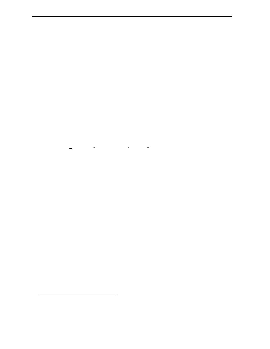
now seems to be). The change in entropy depends on the change of other physical observables
as well, but it is important to realize that in an isolated system (which does not exchange heat or
particles with its surroundings) entropy increases until equilibrium has been reached. After that,
only uctuations will occur and the arrow of time from the entropy gradient will vanish. See
gure 1.1.
It is important to realize that the considerations which led Clausius to formulate the Second
Law, were all phenomenological in nature. He simply observed thermodynamical systems and
generalized their behavior. Theoretical support, starting from contemporary physical theories,
was lacking and Boltzmann was the rst in attempting to derive such a foundation.
1.3 The
H
-theorem
Before we focus our attention on Boltzmann, some interesting results obtained by J.C. Maxwell
should be mentioned rst. He analyzed the behavior of gas molecules in thermal equilibrium.
Using statistical assumptions about the collisions taking place between the molecules constituting
the gas, he proved that a particular distribution of velocities (that is, the frequency with which a
certain velocity occurs in the gas) is stable and therefore describes the equilibrium. This velocity
distribution is called the Maxwell distribution. A link between thermodynamics (the notion of
equilibrium) and statistical mechanics (the assumption about the collisions) was made to arrive
at this conclusion.

14
The Second Law
Boltzmann generalized the result of Maxwell by proving that any initial distribution of velocities
will eventually converge to Maxwell's distribution. The connection between statistical mechanics
and thermodynamics was thus made explicit. However, a price had to be paid for this. Boltzmann's
result relied on an assumption called the Stozahlansatz, which may be stated as follows: the
positions and velocities of the particles are uncorrelated before they collide. In other words, the
velocities of colliding particles do not depend on the fact that they are going to collide. After
collision however, the velocities of the collided particles will be correlated with one another,
namely in such a way that particles with relative high velocities will slow down and particles with
low velocities will speed up. Intuitively one can guess that a Gaussian-like
2
curve will result for
the velocity distribution, which is centered around the velocity corresponding to the temperature
of the gas. The last important step Boltzmann made was to dene a measure describing the
deviation of a specic velocity distribution from equilibrium, which he (later) denoted by
H
.
He showed this quantity to decrease monotonically until equilibrium has been reached and it
therefore could be identied with negative entropy, using an appropriate normalization constant.
The latter result, the monotonic decrease of
H
, became known as the
H
-theorem and is crucial in
arguments concerning the arrow of time exhibited in the evolution of systems from non-equilibrium
to equilibrium (see section 1.5).
How was Boltzmann able to derive an asymmetric principle (the
H
-theorem is explicitly time
asymmetrical) from apparent symmetric assumptions? The question is actually incorrect. The
Stozahlansatz, without the additional assumption of `molecular chaos' after collision, is in fact
time asymmetrical. The justication of the Stozahlansatz is therefore crucial and in section 1.5
we will see under which circumstances it will hold.
Contemporaries immediately raised various objections to Boltzmann's
H
-theorem. Using the
time invariance of the underlying dynamical laws at the microscopic level, one can show (in the
sense of denition 2 of time invariance) that if at a certain moment all velocities are inverted,
the system will revert to the initial conguration (with its velocities inverted). This amounts to
a violation of the
H
-theorem: if a system evolves from non-equilibrium to equilibrium, entropy
increases (and the
H
quantity decreases, satisfying the
H
-theorem) but after reversing all velocities
as described above once equilibrium has been reached, the entropy should begin to decrease and
the
H
-theorem will be violated. Loschmidt pointed this out and the objection thus became known
as \Loschmidts Umkehreinwand" or the reversibility objection. One could object that reversing
all velocities of all molecules of for instance a gas is only theoretically possible (since inverting
a velocity instantaneously requires an innite force) but without an objective direction of time,
actual examples of such a process are not even necessary, as has been pointed out by Price [37,
p. 28]:
\[
:
:
:
], it is worth noting that the atemporal viewpoint provides an irony-proof version
of the objection. Given that there isn't an objective direction of time, we don't need
to reverse anything to produce actual counterexamples of the imagined kind. Any
actual case of entropy increase is equally a case of entropy decrease {which is to say
that it isn't objectively a case of either kind, but simply one of entropy dierence.
(The argument doesn't need actual examples, for it is only the trying to establish
the physical possibility of entropy-decreasing microstates. Lots of things are possible
which never actually happen, like winning the lottery ten times in a row. However,
to understand the atemporal viewpoint is to see that actual examples are all around
us.)"
2
In Dutch this curve is called the `standaard normaal verdeling', known from elementary statistics.

1.4 The rise of statistical mechanics
15
How seriously the
H
-theorem is aected by this objection is clearly shown by Davies in chapter
three of [7]. One can freely construct a distribution function
f
depending only on the absolute
magnitude of the velocities, since the
H
-theorem does not restrict the particular form of
f
. The
value of
f
for any state of the system will be equal to the value for its time reversed state. From
this it follows that if the system resides in a state of molecular chaos then in both directions of
time the entropy should increase and consequently the
H
-theorem can only be valid at a local
entropy minimum. The desired monotonic behavior becomes elusive.
Another objection is based on Poincare's recurrence theorem and will further be referred to as
the recurrence objection. Poincare proved that isolated systems, governed by classical equations
of motion, will eventually return arbitrarily close to their initial conditions (and consequently to
any state in their time evolution). Zermelo pointed out that as a consequence, a system initially
in a low entropy state will eventually return to this state and the
H
-theorem will be violated.
However, the time involved to make a system return to its initial state, the recurrence time, can
be very large compared to the age of the universe. How seriously should we take this theoretical
objection? Using Gibbs' ensemble approach (to be explained later in this chapter), one can show
that the recurrence time for individual subsystems can vary greatly and the ensemble as a whole
will not necessarily return to its initial conguration. However, the ensemble approach itself needs
to be justied, an important issue to which I will return shortly.
The last objection to be discussed here in connection with Boltzmann's
H
-theorem is called
Maxwell's Demon. Maxwell's Demon is an imaginary creature that segregates the slow and
fast molecules of two vessels by controlling an aperture in between. Due to the segregation
of the molecules one vessel will heat up and the other will cool down, again in conict with
Boltzmann's
H
-theorem . However, later (in the twentieth century) it was shown that the amount
of information needed by the Demon to distinguish between slow and fast molecules can account
for the apparent decrease of entropy
3
. Locally, at the Demon, the entropy increase more than
compensates for the entropy decrease in the two vessels: the entropy of the system as a whole
increases and Boltzmann's
H
-theorem will be satised.
1.4 The rise of statistical mechanics
After taking notice of the objections of his contemporaries, Boltzmann began to rethink his theory
and in response developed a statistical interpretation of the equilibrium theory. His main goal was
to reformulate the
H
-theorem such that the reversibility and recurrence objections are avoided.
Using various assumptions, the justication of which is still one of the main problems of the
foundation of statistical mechanics today, he could only show that the
H
value, in a statistical
interpretation, most probably decreases. In his analysis he dened a statistical variant of entropy
that we nd in textbooks today. Entropy is there dened to be proportional to the logarithm
of the number of microstates (the actual positions and momenta of all the individual particles)
that are compatible with a given macrostate of a gas (characterized by temperature, pressure,
etc.). One way to justify this denition is to point to the fact that a macrostate can generally be
realized by a large number of microstates.
In order to gain insight into the rationalization of this alleged reduction of thermodynamics to
statistical mechanics, some rather technical details of his derivation cannot be omitted. Boltzmann
himself was not very clear in the justication of his concepts but P. and T. Ehrenfest reconstructed
it in [11]. I will therefore follow their analysis.
3
Entropy and information are related by the fact that their sum remains equal.

16
The Second Law
The main argument runs as follows: proof that the equilibrium state is the most probable
state of all states in which the system can reside (in the sense that the system will spend most
of its time in this state in the innite time limit), and then show that the system, if it is in a
non-equilibrium state, will evolve very probably towards this state.
The arguments used in both proofs make use of the abstract notions of
;
-space and
-
space that I will explain in this paragraph. Describing a system consisting of many particles
requires the specication of their spatial coordinates and velocities. Real systems `live' in three
dimensions and a particle consequently possesses three spatial coordinates and a velocity vector
of three dimensions. In order to represent a system of
N
particles a six dimensional space can
be constructed with two axes for each degree of freedom. Every particle can now be represented
by one point in this space, called
-space. If, on the other hand, the representation space is
constructed by taking the degrees of freedom of all the particles into account, the system can be
represented by exactly one point. A space constructed in this manner is called
;
-space and would
have
6N
dimensions if the system consists of
N
particles.
The partitioning of phase space into discrete boxes is called coarse-graining and is usually
grounded in the fact that if a measurement is made, in order to determine the microstate of the
system, errors are introduced and the values obtained are only given to lie within a certain error
range. In
-space every box contains a specic number of particles, the occupation number. The
total set of occupation numbers form the so-called state-distribution. It should be clear now that
a state distribution does not completely specify the microstate of a system but only determines
the range of microstates in which the system must reside. Therefore, the associated region of
;
-space of a state-distribution will not be a point, as would be yielded by an exact microstate,
but a nite volume.
We can now proceed to the proof of the rst issue, namely that the equilibrium state is the
most probable state of all states in which the system can reside. It depends on the fundamental
postulate of statistical mechanics: in the absence of any information about a given system, the
representative point is equally likely to be found in any volume of
;
-space. Now, what exactly
does this mean? The whole volume of
;
-space represents all the states physically accessible. If
one knows nothing about the system then it is equally likely to be found in any region of this
volume. Since the volume of the equilibrium state-distribution occupies the largest fraction of
;
-space, equilibrium will be the most probable state. In order to guarantee that the system will
actually spend most of its time in this state, another assumption must be used, the Ergodic
Hypothesis: the trajectory of a representative point eventually passes through every point on
the energy surface
4
. Since most points on the energy surface will correspond to the equilibrium
state-distribution, the system will spend most of its time in equilibrium.
The last issue to be proved is that a system, if it is in a non-equilibrium state, will evolve very
probably towards equilibrium. This can be shown as follows. Suppose the system resides in a
region of
;
-space for which
H
is not at a minimum (or similarly: entropy is not at a maximum).
Now consider the ensemble consisting of the all points within the volume of
;
-space corresponding
to the state-distribution of the system. The evolution of all these representative points is xed
but since the volume of
;
-space associated with equilibrium is largest, it is very likely that most
points will start to evolve towards this region. Now, the entropy for the state, which is achieved
at each instant of time by the overwhelmingly greatest number of systems, will very probably
increase. The curve obtained in this manner is called the concentration curve.
At rst sight the decrease of the concentration curve seems to reestablish an
H
-theorem
4
The energy surface is a region of
;
-space in which the energy of the system remains constant.

1.5 Non-equilibrium phenomena
17
free of reversibility and recurrence objections but there turn out to be many problems. The
arguments of Boltzmann by no means show that the most probable behavior is the actual or
necessary behavior of a system. Secondly, a monotonic decrease of
H
along the concentration
curve requires a construction of ensembles of representative points according to the fundamental
postulate of statistical mechanics at every instant in time. The use of the postulate in this
manner must rst be shown to be legitimate and is in fact in contradiction with the deterministic
character of the underlying laws of dynamics. Thirdly, the reasoning involved in establishing the
statistical interpretation of the
H
-theorem is perfectly time symmetrical. The consequence of this
(as pointed out by E. Culverwell in 1890) is that transitions from microstates corresponding to
a non-equilibrium macrostate to a microstate corresponding with an equilibrium macrostate are
equally likely to occur as reverse transitions.
The third problem led Boltzmann to formulate his time symmetrical picture of the universe.
In this picture he still supports the view that a system in an improbable state is very likely to
be found in a more probable state (meaning closer to equilibrium) at a later stage, but now we
must also infer that it was closer to equilibrium in the past. The entropy gradient in time has
disappeared. In order to explain the present situation, in which we nd ourselves, he turns to
cosmological arguments, which I will not discuss in this paper.
The turn towards a time symmetrical universe is by no means the only `solution' of the
problems concerning the concentration curve. Price however embraces it and urges that the main
question should be: `Why is the entropy so low in the past?' There are many other arguments
in establishing the time asymmetry of the Second Law besides the very general one delineated
above. In the next section I will analyze these methods and especially address the question how
time asymmetry itself is established by these methods.
1.5 Non-equilibrium phenomena
Earlier in this chapter we encountered a very intuitive example illustrating the irreversibility of the
Second Law. It ran as follows. If one adds some blue ink to a glass of water and starts stirring,
then after a while this will result in a homogeneous light blue liquid. The feature of interest in
this process is its irreversibility. Before the compound liquid of the water and ink was disturbed,
the system resided in a non-equilibrium state. When the ink and water mixed due to stirring,
the system approached equilibrium and the emergence of the light blue liquid marked the nal
equilibrium state.
This is a very natural phenomenon, one would be inclined to think. But how can one account
for this process physically? In this case the presence of external forces, caused by the stirring, adds
some complications, but even in the case of an isolated gas initially in a non-equilibrium state, to
predict the resulting behavior has been proven to be very dicult. Many problems occur if one
tries to make a prediction. The enormous amount of particles and our inability to measure the
initial coordinates and velocities of all the particles precede the fact that given such data, solving
the time evolution of such a system is impossible, even with the aid of current supercomputers.
The goal of statistical mechanics is to account for the evolution of thermodynamic quantities
while precisely avoiding such calculations. In the case of systems residing in equilibrium, the
theory is quite successful but its extension to non-equilibrium phenomena is not straightforward.
The rst problem is the wide range of behaviors displayed in non-equilibrium phenomena. Even
the emergence of order can occur in systems residing far from equilibrium. Prigogine describes
such examples of self-organization in great detail in [38]. A grounding theory, based on the

18
The Second Law
dynamical laws governing the behavior of the micro-constituents and perhaps some additional
fundamental assumptions (which would have to be proved), would have to explain the behavior
of all these phenomena. Most theorists only focus their attention on the problem of the approach
to equilibrium, as we will see later in this chapter, a phenomenon which in itself is hard enough
to explain.
Another fundamental problem is which denition of entropy to use within a theory. In the
previous section we encountered the concept of coarse-graining, i.e. the partitioning of phase
space into discrete boxes. Many authors object that this concept is somehow 'subjectivistic'
because it is essentially based on our limited abilities to measure the state of a system exactly.
Yet without the use of coarse-graining it can be shown that the entropy will remain constant (!),
due to the important theorem of Liouville.
Now, what would a theory describing the approach to equilibrium look like? There are various
ways to describe the initial state of a non-equilibrium system. One could provide a set of ther-
modynamical observables whose values depend on the coordinates within the system. The aim of
the grounding theory in this case is to provide a sort of scheme to derive the time evolution of the
observables involved. A successful theory would thus account for the important time-asymmetry
of many macroscopic phenomena.
In this section I will examine some attempts at establishing such a theory. The rst part of
this chapter will deal with theories explaining the approach to equilibrium. The success of these
theories depends in a way on the degree of chaos that is exhibited by the system in question.
Claims about the evolution of thermodynamic observables are only valid when one has rigorously
proven that the system is indeed chaotic with respect to some standard. Sklar speaks in this
context of the justication of the use of some rerandomization posit [44]. Nevertheless, even if
one can prove that the system behaves chaotically with respect to some standard, one would still
have to deal with the recurrence and reversibility objections to justify the use of a specic theory.
Why is the use of a rerandomization posit successful when applied to one direction of time and
not for the reverse direction? Several attempts to explain the macroscopic time-asymmetry will
be reviewed.
1.5.1 The ensemble formalism
The several statistical theories which oer an approach to the derivation of the kinetic behavior
of a system in non-equilibrium are all based on the use of ensembles to describe the current state
of a system. The ensemble formalism will therefore be outlined in this section.
Initially developed by Maxwell and extended mainly by Gibbs, the ensemble formalism is
regarded as a very useful tool to analyze the properties of many particle systems. An ensemble
is a large number of mental copies (meaning that they interact in no way with each other) of
a single system. Usually, an ensemble is constructed is such a way that all the members of the
ensemble have the same macrostate but a dierent microstate. Each copy will have an associated
representative point in
;
-space, so that the whole ensemble will be described by a cloud or swarm
of points, all moving together in a complicated fashion. The swarm of points can actually be
treated as a uid in
;
-space because the theorem of Liouville earlier mentioned, which states that
if the evolution of the members of the ensemble is governed by the classical equations of motion,
the uid is incompressible. The density of the uid is described by the so-called probability density
function, which indicates the probability that the system is found in a particular region in
;
-space.
A correct probability density function describing equilibrium should be stationary (this is ac-
tually the very denition of statistical equilibrium) since all macroscopic parameters are supposed

1.5 Non-equilibrium phenomena
19
to remain constant if the system is in equilibrium. For an isolated system in equilibrium, a certain
probability distribution (the micro-canonical distribution) is known to be stationary, but one of
the main problems in equilibrium theory is to show that this probability distribution is the only
stationary distribution. If it were not the only stationary distribution, the recipe for calculating
equilibrium values of thermodynamic quantities using this distribution would be unjustied.
This recipe for calculating equilibrium values is straightforward, this in contrast to its full justi-
cation. First an ensemble must be created which is compatible with the macroscopic constraints.
Given the xed energy of the system, an appropriate stationary probability density function com-
bined with an invariant volume measure over
;
-space should be constructed. The value of any
phase function (that is, a function depending on the coordinates in phase space) can now be
obtained by integrating the product of the phase function and the probability density function
with respect to the volume measure. The quantity obtained in this manner is the ensemble aver-
age of the phase function. Gibbs formulated a phase function analogy for every thermodynamic
quantity, but whether the ensemble average of a phase function coincides with the thermodynamic
equilibrium value remains an unsettled issue. A number of assumptions is used in justifying this
equality, but the feature of ergodicity is by far the most important one. I will discuss this concept
in some detail here because it will return.
In the previous section the Ergodic Hypothesis was briey mentioned. This original formulation
of ergodicity was later proven to be too strong in the sense that no single system could comply
with it. A weaker version, the so-called Quasi Ergodic Hypothesis, turned out to be insucient
to gain the result desired, that is, the equality of the ensemble average and time average of a
phase function. Von Neumann and Birkho nally found a suitable constraint for the dynamics
of a system that ensured that this equality would hold: metric indecomposibility
5
of phase space.
Problems persisted, however. For realistic systems it is very hard to prove that they behave
ergodically. Some progress has been by Sinai on systems showing much resemblance with realistic
systems, but there is a theorem (the KAM theorem
6
) that indicates that even when interacting
only weakly, many particle systems may have regions of stability in phase space, in contradiction
with the ergodic hypothesis.
Now we can focus our attention on the theories explaining the approach to equilibrium.
1.5.2 The approach to equilibrium
How does statistical mechanics establish the apparent time-asymmetry in thermodynamical sys-
tems as they approach equilibrium? In order to gain insight into the answers various theories
provide, the theories themselves will have to be elucidated. A single theory describing all the
phenomena displayed by systems residing far from equilibrium is not available. Progress has been
made, but contemporary theories oer at best an approach to a possible `solution'.
The procedure to predict the evolution of a system initially not in equilibrium is quite clear.
The rst step is to dene an initial ensemble. A set of macroscopic parameters must be chosen
to restrict the available phase space and an appropriate probability density should be assigned
5
Metric indecomposibility of phase space entails that the phase space cannot be divided into subspaces of nite
volume containing trajectories that will remain within such a subspace.
6
The KAM theorem has been proven by Kolmogorov, Arnold and Moser and roughly states that a system
satisfying certain conditions will not show ergodicity under weak perturbations. The unperturbed system must
consist of a number of non-interacting subsystems whose eigenfrequencies ratios are not integers. Without a
perturbation such a system is not ergodic. People were strongly convinced that a perturbation would cause the
system to behave ergodic but Kolmogorov, Arnold and Moser proved this not to be the case. See Chapter 4 of [1]
for more details on the KAM theorem.

20
The Second Law
over this restricted part of phase space. The next step consists in following the evolution of this
ensemble by means of a kinetic equation, which has the proper time-asymmetry and monotonicity
to represent the approach to equilibrium. The last step will be the calculation of the phase
function associated with the thermodynamical observable one wishes to measure by taking its
ensemble average. Serious diculties present themselves in each step of this procedure but the
second step, the use of a kinetic equation, or actually the derivation and justication of the kinetic
equation, will be the subject of this section.
The behavior of the initial ensemble is xed in principle, provided that the interaction laws
between the particles are known and that the process is completely isolated. However, approxima-
tions and assumptions will have to be made if one does not wish not to solve the evolution solely
using the basic interaction laws and Newton's equations of motion. The assumption usually made
somewhere in the derivation of a kinetic equation is a generalization of the hypothesis of molec-
ular chaos. One assumes that the ensemble has evolved in such a way that at a given time the
macroscopic parameters have such a value that the future evolution could be predicted correctly
if one started with a random ensemble compatible with the macroscopic parameters. Sklar calls
this process `rerandomization' and explores three dierent approaches to derive a kinetic equation
in chapters 6 and 7 of [44]. The attention in the discussion of every approach will be focused on
the question where rerandomization is used and how it is justied:
Kinetic theory approach.
In this approach one approximates the ensemble by a partial descrip-
tion that allows the computation of macroscopic observables. The aim of this theory is to
be able to formulate a closed dynamics for this partial description. In the so-called BBGKY
approach this approximation is being made continuously and constitutes a variant of the
hypothesis of molecular chaos. Here we nd the rerandomization posit and the ultimate
source of time asymmetry. The main objection lies in the fact that the neglected part of the
ensemble does not always behave as `smoothly' as required for the approximation to be jus-
tied. A more rigorous version has been formulated by Lanford. Here the rerandomization
occurs initially by again taking the partial description instead of the full ensemble. Lanford
was able to derive a kinetic equation without any further assumptions, but the restrictions
under which this equation holds make it inapplicable to real systems.
Master Equation approach.
The rst assumption one makes is that the system consists of a
set of weakly interacting subsystems. Secondly, it is presumed that the probability of energy
leaving or entering a region of modes is proportional to the spread of that region and remains
constant. Constant probability indicates a continuous rerandomization. Aside from some
other restrictions, this approximation is only valid in the innite time limit, which restricts
its applicability to real systems rather seriously, since relaxation times
7
of less than a second
are known. Besides this, the KAM theorem applies to precisely this category of systems
and may impose additional restrictions on the use of this approach.
Coarse-graining approach.
The foundations for this approach were laid early in the development
of statistical mechanics. If one can show that trajectories in phase space are continuously
unstable with respect to some measure of chaos, then the assumption that a Markov process
8
accurately describes the dynamics may hold. Using the Markovian assumption, a kinetic
equation can be derived indicating an approach to equilibrium in the coarse-grained sense.
7
The relaxation time of a system in non-equilibrium is the time needed for the system to stabilize to equilibrium.
8
The Markovian postulate states that the probability of the transition of a representative point from one box in
phase space to another box is proportional to the number of points in the rst box.

1.5 Non-equilibrium phenomena
21
Several problems can be signalled in this approach. The argument for coarse-graining must
be rationalized more thoroughly than the intuitive reasoning mentioned earlier. Secondly,
one must show why the Markovian assumption works in accurately describing the dynamics
of the system (when it works) since it is incompatible with the deterministic character of
the actual evolution of the ensemble. And thirdly, in order to legitimise the use of the
Markovian assumption, one must show that the system behaves chaotically with respect to
some measure, which is by no means a trivial exercise.
Some general remarks concerning the derivation of a kinetic equation should be noted at this
point. The three approaches outlined above are all restricted in some sense, and use unproved
assumptions. Even if one of the approaches holds and successfully provides a kinetic equation,
what are then the implications for time-asymmetry? The kinetic equation describes the time
evolution of macroscopic observables, in the sense of a `concentration curve' of an ensemble evo-
lution. What can we then infer about the behavior of an individual member of the ensemble from
the concentration curve? Some members may evolve to a state further away from equilibrium,
whereas others may indeed show an approach towards equilibrium. On average, the concentration
curve will be followed. This picture is completely compatible with the recurrence theorem. As
long as the recurrences of the individual members are incoherent, i.e. are not taking place at
the same time, the ensemble as a whole can follow the concentration curve. However, the other
major objection against time-asymmetry, viz. reversibility, still holds. Why should a rerandom-
ization assumption be applied to one direction of time and not to the reverse direction? If the
rerandomization posit itself is not taken to be fundamentally time asymmetric, then the source of
time asymmetry must be found elsewhere. In the next chapter I will analyze two such attempts:
interventionism, which takes the system not to be totally isolated, and several theories that exploit
the initial conditions.


Chapter
2
Time Asymmetry and the Second Law
2.1 Introduction
In the previous chapter I have attempted to demonstrate how dicult it is to establish a theory
predicting the approach to equilibrium of a system initially not in equilibrium. Even if one accepts
one of the various accounts that were mentioned, another more fundamental problem still persists:
the time asymmetrical character of such phenomena. I have delineated where time asymmetrical
assumptions are `inserted into' the theories. They turned out to be rerandomization posits, i.e.
generalizations of the assumption of molecular chaos from Boltzmann, applied either to the initial
state of a system or continuously during its evolution in time. Now, if one refrains from taking
such assumptions to be fundamental (law-like) time asymmetries, the reversibility objection still
holds. The main question then becomes: why do only those initial states that lead to an increase
in entropy occur in nature? One implicitly accepts that anti-thermodynamic behavior (meaning
a decrease in entropy) of a system is allowed, but simply does not occur, or is too unlikely to
occur. Before turning to the theories that exploit the initial conditions, I will try to make clear
what anti-thermodynamic behavior entails in some detail.
In the previous chapter the concept of phase space was briey mentioned. Simple systems,
typically consisting of one particle in a two dimensional potential, can be analyzed by making
phase space portraits of their time evolution. If the potential is conservative, the total energy will
remain constant and the evolution of the system will be restricted to take place in a limited part
of the whole phase space. Now the phase space portrait of a system like a pendulum is a simple
curve, leaving the available phase space almost entirely uncovered. The trajectory of an ergodic
system on the other hand will eventually pass arbitrarily close to any point in the available phase
space.
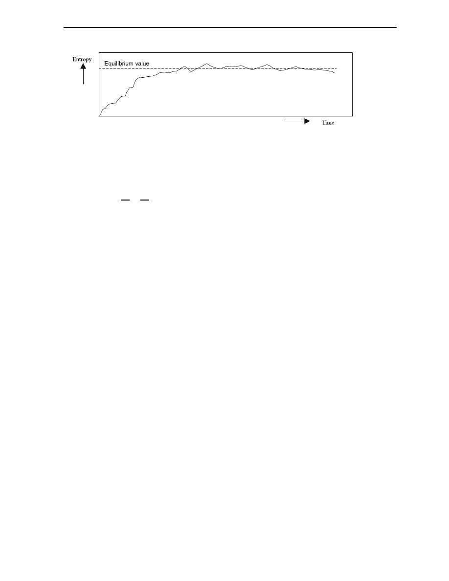
In the ensemble formalism one analyzes not the trajectory of one point in phase space, but
a whole region of points. Every point has a probability assigned to it, representing the chance
that the system will be found in the corresponding state. Initially the region is constructed in
such a way that each individual member of the ensemble satises a dierent microstate but the
same macrostate. The probability density is usually uniformly distributed over the region. The
trajectory of each point is xed, due to the deterministic nature of underlying dynamical laws
and at a later time the points will have spread. See gure 2.1. Note that the surface of the
region as displayed in the picture remains constant, due to Liouville's theorem. This indicates the
constancy of ne-grained entropy.
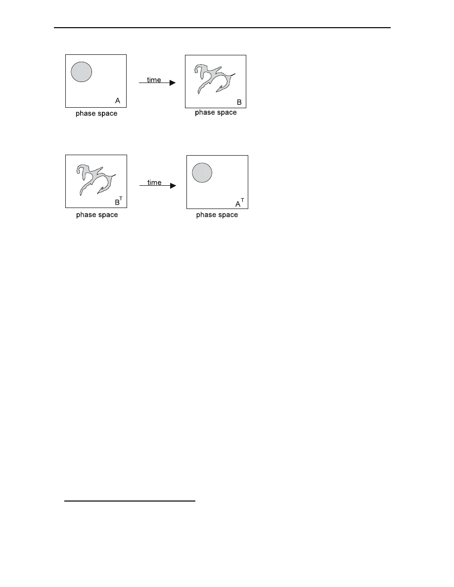
Since the trajectories of all representative points are time reversible, the ensemble construed
24
Time Asymmetry and the Second Law
Fig.
2.1:
Time evolution of a system in phase space
Fig.
2.2:
Time reversed evolution of a system in phase space
by taking the time reversed states of all the points in the second picture (B) should evolve back
to the rst picture (where B
T
and A
T
denote the time reversed states). See gure 2.2. What we
see here is reversibility at the ensemble level. The transformation of B
T
to A
T
could be described
as anti-thermodynamic since the coarse-grained entropy clearly decreases. The complex form of
B
T
required for the anti-thermodynamic behavior to occur is regarded as improbable. Standard
statistical mechanics uses the postulate of equal a priori probabilities
1
to justify this claim. Now
the central problem is reduced to the requirement to give an explanation why such a complex
initial condition that leads to anti-thermodynamic behavior, does not occur in nature.
At this point it should be noted that indeed an experiment can be conceived where the
process of time reversal can be carried out. In an experiment which became known as the spin-
echo experiment, the alignment of nuclear spins in a magnetic eld can be manipulated. In the
initial conguration all spins are set up in correlation with each other, but after a while many
spins will be oriented in a random direction. Now by means of a radio-frequency pulse the spins
can be ipped and the system will evolve back to the original conguration. The analogy with
Loschmidt's original reversibility objection is quite obvious. In this case it is not the velocities of
the molecules, but rather the axis of rotation of the spins that are inverted. The eect is the
same: the system can be made to evolve back to its initial state, even from a macroscopically
`chaotic' state.
To see more clearly what is going on in such processes, the relation between entropy and infor-
mation will have to be made more explicit. Our knowledge about specic macroscopic properties
of a system is generally described by macroscopic information, this in contrast with knowledge
about microscopic correlations between molecules, which is called microscopic information. If
the initial condition is known only in macroscopic terms (which is typically the case for non-
equilibrium systems), then the initial macroscopic information has a specic non-zero value. The
1
This postulate states (see Chapter 1): in the absence of any information about a given system, the representative
point is equally likely to be found in any volume of
;
-space.

2.2 Interventionism
25
microscopic information is absent in such a case. This fact is reected in the choice of assigning
a uniform probability density to the microstates of the initial ensemble. After a while, the system
will have evolved to a new state, probably closer to equilibrium. When the system has reached
equilibrium, the macroscopic information will have disappeared, since all macroscopic observables
will have a uniform value throughout the system. The information has not been lost, however:
it has been transformed into microscopic knowledge, i.e. specic knowledge about correlations
between individual molecules. The presence of this knowledge in the system is reected in the
spin-echo experiment. If knowledge about the initial conguration was not present somewhere in
the system, it could never evolve back to this state.
Some people are convinced that microscopic knowledge is also lost in equilibrium, and that
`true' equilibrium is only reached when reversibility is impossible. How this interventionistic ap-
proach tries to solve the problem of the approach to equilibrium and time asymmetry will be
analyzed in the next section.
2.2 Interventionism
Not a single thermodynamical system, the universe as a whole excluded, can be considered com-
pletely isolated. In the case of a gas in a vessel, there will be interaction between the walls and
the gas through collisions besides the gravitational interaction with the rest of the universe. No
one will doubt these facts, but can they somehow be used to solve some of the puzzles we have
encountered so far?
First of all, one should not overestimate the inuence the outer walls have on a gas. The
relaxation time for the combined system (container and gas) to reach equilibrium can be up to
104 times as large as the relaxation time for the gas itself to reach internal equilibrium. What
would we like to obtain by invoking such small perturbations? Can they somehow break the
conservation of ne-grained entropy or even of time symmetry itself?
Davies discusses this issue by presenting interventionism as an alternative to the coarse-
graining approach for entropy increase. Maybe, if one can show that ne-grained entropy indeed
increases, and microscopic correlations are subsequently destroyed, then the `subjective' concept
of coarse-graining is unnecessary. It is indeed true that the ne-grained entropy of the system
consisting of a gas and its `intervening' walls will increase, but Davies points out that there is
no real conict between this picture and the coarse-graining approach to entropy increase. Each
description applies to a dierent conceptual level. Coarse-graining applies to the macroscopic level
of observation and the associated entropy can be proven to increase if microscopic correlations
are continuously thrown away, something Davies describes simply as `what is actually observed'
[7, p. 77]. He justied this earlier with the remark: \
:
:
:
statistical mechanics is precisely a
macroscopic formalism, in which macroscopic prejudices, such as the irrelevance of microscopic
correlations, are legitimate." On the other hand, we see that the increase of ne-grained entropy
occurs at microscopic level, due to interventionism, and it is at this level of description where
the random perturbations from outside cause irreversibility. According to Davies: [idem] \
:
:
:
attempts should now not be made to use the undeniable existence of this micro-irreversibility to
discuss the question of asymmetry at macroscale." He concludes that interventionism does not
oer an alternative for coarse-graining but merely a description at a dierent conceptual level.
In his account of interventionism, Sklar [44] also doubts the results that can be obtained using
intervention from outside. The spin-echo experiment shows that even in the provable absence
of loss of microscopic correlations, there is still some loss of information unaccounted for by

26
Time Asymmetry and the Second Law
interventionism, since the system becomes more chaotic at macroscale. As for interventionistic
arguments proving time asymmetry, Sklar does not see how they can escape the parity of reasoning
mentioned in Chapter One, since random perturbations that would lead to time asymmetries would
have to be time asymmetrical in themselves, a posit that would have to be justied.
2.3 Initial conditions
I will not analyze the route to asymmetry by means of the structure of probabilistic inference as
understood from a subjectivistic or logical theory of probability point of view. Gibbs explored this
possibility by observing that we often infer future probabilities from present probabilities, but that
such inference with respect to the past is illegitimate. Instead I will concentrate on Krylov's and
Prigogine's investigations on the nature of initial ensembles.
2.3.1 Krylov and the preparation of a system
In the introductory section to this chapter it has been emphasized that the usual way in statistical
mechanics to describe the initial ensemble is by means of a uniform probability density assigned
over the appropriate microstates. Such a description will not lead to ensembles behaving anti-
thermodynamically. But how does one justify this choice? Krylov is not satised by the statement
that the existence of such initial conditions (and subsequently their statistical characterization) is
a `mere fact about the world' [23]. He thinks that this choice can be based on our limited abilities
to prepare the initial state of a thermodynamical system. For neither quantum theory nor classical
mechanics provide any restriction on our ability to prepare systems in such a way that only the
appropriate kind of initial ensembles is ever allowed to be representative of the system's initial
state. Krylov invokes the ineliminable interaction of the preparer with the system that is being
prepared to justify his claim. It is the ineluctably interfering perturbation, which occurs when a
system is being set up initially, that guarantees that the appropriate statistical description of the
system will be a collection of initial states that is suciently large, suciently simple in shape,
and with a uniform probability density distribution assigned to it. When combined with the (to
be proven) instability of the trajectories characterizing the system to be chaotic with respect to
some measure, these circumstances can hopefully lead to an entropy increase in the coarse-grained
sense, and time asymmetry is reached.
There are various arguments against this line of reasoning. The spin-echo experiment men-
tioned earlier showed that it is indeed possible to prepare a system in such a way that it will
show anti-thermodynamic behavior, but, strictly speaking, Krylov did not claim that this was
impossible. Secondly, the precise notion of the preparation of a system remains problematic. How
does Krylov escape the parity of reasoning? What makes the preparation of a system dierent
from the destruction of it other than by means of causal arguments? Reference to causality to
found the arrow of time of the Second Law cannot be the argument Krylov tries to make, but I
see no way to avoid this reference.
2.3.2 Prigogine and singular ensembles
In a rather mathematical framework, Prigogine tries to establish time asymmetrical behavior in
thermodynamical systems by permitting only a specic kind of ensembles, viz. `bers', as initial
ensembles. He shows that such an ensemble and its evolution can be transformed by a so-called
non-unitary transformation and that the evolution of the newly obtained representation can be

2.4 Branch systems
27
described by a Markovian type time asymmetric kinetic equation. The ensembles he allows as
appropriate initial ensembles are singular
2
and will approach equilibrium in one time direction and
not the other!
The bers come in two kinds: `contracting' and `dilating'. Both kinds t the above mentioned
requirements but the choice to use only the dilating one is justied by the fact that the entropy
for this ber will remain nite and can be prepared physically (at least in principle), whereas the
entropy for the contracting ber goes to innity as time increases and is impossible to prepare.
Prigogine's derivation of time asymmetry may seem promising but again there are objections.
To prove that a real system behaves like a ber is mathematically very dicult. And besides the
fact that it is practically impossible to prepare singular ensembles, Prigogine's whole derivation is
aimed at the derivation of thermodynamic (in the sense of irreversible, time-asymmetric) behavior
by allowing the appropriate ensembles to be a `good' description of the initial state while others
are not. The ultimate justication for this particular choice, which is even in conict with the
results of the spin-echo experiment, remains unclear to me.
2.4 Branch systems
An attempt to derive the arrow of time of the Second Law from cosmology is found in the branch
system mechanism, originally developed by Reichenbach [39] and later supported by Davies [7].
Branch systems are regions in the world that separate o from the main environment and exist
thereafter as quasi-isolated systems, until they merge again with the environment. Nobody doubts
the fact that the systems with which we deal in thermodynamics are branch systems. However,
the problem is to exploit this fact to explain the entropy gradient and especially the parallelism of
the direction of this gradient in all thermodynamic systems. In this context I want to emphasize
the fact that not only the entropy gradient itself needs explanation, but also the fact that this
change is always positive.
From cosmology it is known that the current entropy state of the universe (at least the part
we can observe) is extraordinary low and increasing with time. Using this fact, one might try to
prove that the direction of entropic increase in branch systems is the same as the direction of
increase in the universe as a whole, and always occurs in parallel directions with respect to time.
I will analyze the attempts of Reichenbach and Davies to establish this.
The crucial point in their derivations of entropic increase and parallelism will turn out to be
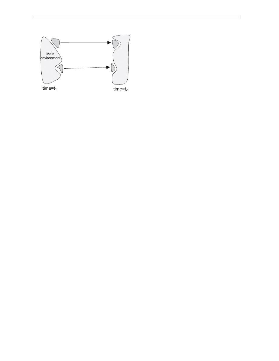
why certain assumptions are claimed to hold during the formation of branch systems and not
during their destruction. How should we distinguish between the formation and destruction of a
branch system other than on causal or temporal grounds? See gure 2.3.
In the above picture we see two branch systems being formed by isolation from the environment
at time equals
t
1
. After both systems have evolved in quasi isolation, they eventually merge again
with the main environment, at time equals
t
2
. The picture suggests that
t
1
corresponds to the
`formation' of the branch systems and
t
2
to the `destruction', but when the information whether
t
1
is earlier than
t
2
or not is unavailable, this need not to be so. Indeed, in the absence of this
information, the usual statistical description of initial states would have to be justied and is
crucial to establish the entropy gradient. In order to establish a parallel entropy gradient, the
statistical description of initial states should only be applied to branch systems being formed and
2
Singular ensembles form a set of measure zero. As an illustration, consider the fact that a set of points will
never cover a surface (or volume), since a point has no spatial dimensions (only coordinates). Ensembles of measure
zero likewise form a group of points in phase space and no continuum. Such a set can never be prepared since
some uncertainty will be introduced in one or more of the canonical variables.
28
Time Asymmetry and the Second Law
Fig.
2.3:
Formation and destruction of branch systems
never to branch systems being destroyed, and again, without reference to causal or temporal
arguments it is not clear how one can distinguish between the two events. In the following
discussion of Reichenbach's and Davies' theories of branch systems I will show that they fail to
solve this problem.
2.4.1 Reichenbach's lattice of mixture
Reichenbach tries to establish the parallelism of the entropy gradient of branch systems by starting
from various assumptions. The most crucial assumption reads: `the lattice of branch systems is a
lattice of mixture'. What does this exactly mean? Consider a large collection of similar systems
that evolve over identical periods of time. Now, some macroscopic observable is measured for
each system at small, equal intervals of time as the systems evolve from their starting point. The
lattice of branch systems is construed by inserting a row of such values for each system. The
`mixture' feature is dened as a set of mathematical properties but essentially comes down to
constructing the lattice in a very special way. The time order of the states in the left-hand column
with respect to the states in the right-hand column is nearly always the same, meaning that the
low-entropy ends (and similarly the high-entropy ends) are distributed over the same columns.
Parallelism is thus explicitly inserted.
Since the main environment from which the branch systems separated is itself a branch system,
it will have its entropy increase in the same direction as that of the bulk of other systems. The
entropy gradient in branch systems will therefore be in the same time direction as in the main
environment.
Although Reichenbach himself did not explicitly claim to explain why the entropy gradient in
branch systems is parallel, he seems to suggest this. In the above analysis I have shown that the
parallelism, in my opinion, is not derived from some more fundamental principles, but explicitly
inserted by the apparent innocuous `lattice of mixture' assumption.
2.4.2 Davies' non-existing prior states
The line of reasoning Davies follows to establish the parallelism in branch systems is quite clear. If
a low entropy state is selected at random when the branch system is formed, it will most probably
evolve to a higher entropy state, in both directions of time. Now, since it is formed in a low
entropy state, it did not exist in the past, and the entropy cannot decrease in that time direction,
but only the future time direction. In addition, he claims that parallelism arises due to the fact

2.5 Conclusion
29
that all the low entropy states are formed randomly, and the overwhelming majority will therefore
show an entropy increase in the same-parallel-time direction. Davies grounds the ultimate time
asymmetry in this way on the formation of branch systems, and not on a statistical assumption,
coarse-graining or anything else.
Again, the time asymmetry is in my opinion explicitly inserted by claiming that ensembles are
formed randomly and not reabsorbed randomly: Davies only considers the moment of creation,
and applies the rerandomization posit at this event. The subsequent evolution to a higher entropy
is not strange. But when the branch system is nally reabsorbed into the main environment, not
such assumption is said to hold (in fact, he does not consider the reabsorption at all). The
justication for this choice is absent. Again, if no objective direction of time is given, to speak of
the creation of a branch system is the same as to speak about its destruction.
2.5 Conclusion
The analysis of the various approaches to establish time asymmetry from the initial conditions of a
system demonstrated that especially the parallelism of the entropy gradient remains a phenomenon
that is very hard to prove. Many authors take it for granted that the arrow of time of the Second
Law can be derived from the arrow of time in cosmology, using for example the branch system
mechanism. In this chapter, I have showed that this `derivation' is not as trivial as it seems to
be. Dierent contemporary approaches, whether or not relying on this connection and providing
an answer for the problem of the asymmetry of the Second Law, will be the subject of the last
chapter.


Chapter
3
Contemporary discussions
3.1 Introduction
The problems related with the asymmetry of the Second Law have been claried in the previous
chapters. At some points the 'solution' an author oered has been analyzed, but his solution
turned out to be not as irrefutable as intended. A `good' theory (as mentioned at the end of the
introductory chapter) should be grounded in facts, principles or fundamental laws nobody doubts.
Such a theory is obviously lacking, but in this chapter I will discuss three theories that claim
this status, now that we have familiarized ourselves with the language and concepts in which
these theories are presented. The rst theory, which is presented by Coveney and Higheld in the
chapter `A unied vision of time' of [6], relies on chaos theory to make the postulate to place
the Second Law and (classical) mechanics on equal footing less ad hoc. David Layzer, on the
other hand, appeals to cosmological, information theoretical, arguments to derive an asymmetrical
arrow of time in [25] and Price nally claims that the `atemporal viewpoint' will give more insight
into what the `real' problem is. In the following sections I will analyze these theories in greater
detail, after which I will make some concluding remarks. Yet, I will not be able to oer a solution
and I am afraid I shall be in good company in this respect. Nevertheless, I do hope that I have
claried some of the fundamental problems involving the time asymmetry of the Second Law and
have provided some useful comments on the approaches of other authors. The discussion of the
Second Law and the arrow of time being nished, I will procede in the next part with the arrow
of time in cosmology.
3.2 Cosmology and information theory
In an article in Scientic American [25], David Layzer presents an unorthodox theory concerning
the arrows of time in both thermodynamics and cosmology. He identies two phenomenological
arrows of time that are in conict with one another at rst sight. The historical arrow of time
emerges through processes generating order or information, by transforming a simpler state into
a more complex one. The thermodynamical arrow of time on the other hand is dened by the
irreversible destruction of macroscopic order. Layzer argues that neither of the arrows of time
can be observed at the microscopic level or are required by fundamental laws but that they can
instead be derived from auxiliary assumptions about the nature and origin of the universe. These
assumptions can be replaced by simpler ones and in the resulting model the apparent contradiction
between the two arrows of time are resolved and reconciled with the time symmetrical physical

32
Contemporary discussions
laws. We shall see how Layzer tries to establish his ambitious claims.
In an earlier chapter in this paper we saw that in an irreversible process macroscopic information
is converted into microscopic information. The rst non-trivial claim Layzer makes in his article,
and generally believed to be true, is that for certain kinds of physical systems under certain initial
conditions it can be shown that this irreversibility is inevitable. Furthermore, he claims that the
entropy (identied with negative macroscopic information) of a closed system will only increase if
macroscopic information is initially present in the system and microscopic information is initially
absent. In order to explain why microscopic information is only present in nal states and not in
initial states, he argues that microscopic information is in fact not present in nal states, but is
dissipated through interaction with the environment. Therefore, the initial condition is perpetually
re-created to ensure the decay of macroscopic information and the increase of thermodynamical
entropy. This account of irreversibility was encountered earlier as interventionism.
Interventionism does not apply to the universe as a whole (since it is indeed isolated if it is
nite). Layzer explores a dierent route to prove the asymmetric evolution of the universe as
a whole. Note that he does not establish a connection between the cosmological and thermo-
dynamical arrows of time. The main argument runs as follows: if one can prove that at the
initial singularity microscopic information was absent and macroscopic information either absent
or minimal, then due to the expansion both entropy and macroscopic information are generated,
and the cosmological arrow of time is established.
In order to prove the absence of microscopic information at the initial singularity he appeals
to the strong cosmological principle. This principle states that the spatial distribution of matter
in the universe is homogeneous and isotropic, apart from local irregularities, which themselves are
statistically homogeneous and isotropic. Now, since the initial singularity satises the strong cos-
mological principle, microscopic information was initially absent. For if there was any microscopic
information to distinguish a particular position or direction, it would repeat itself at another loca-
tion and would therefore be ambiguous. This argument may sound cryptic but Layzer elaborates
this point by using an analogy with a so-called `toy universe', which I will not repeat here.
Concerning the absence or minimum of macroscopic information he proceeds as follows. Sup-
pose the universe is in equilibrium and expands or contracts, then there are two possible situations.
Either the equilibrium rates of physical processes are high enough to maintain equilibrium or they
are not high enough and as a consequence local departures from equilibrium will appear. In both
cases macroscopic information (here dened as the dierence between the actual value of the
entropy and the theoretical maximum value at the mean temperature and density) as well as
entropy will increase. In the period immediately following the singularity, the rates of equilibrium
processes are much higher than the rates of cosmic expansion. After that, the system will not
remain in equilibrium and both entropy and macroscopic information will be generated. Layzer
now concludes that from the assumptions of the strong cosmological principle and of a prevailing
thermodynamical equilibrium at or near the initial singularity, the historical and thermodynamical
arrows of time will follow.
Many aspects of the derivation of Layzer remain unclear to me. The most crucial point is,
in my opinion, the absence of the connection between the cosmological and thermodynamical
arrows of time. It is one thing to prove, or make it likely, that microscopic information is initially
absent, but how this ensures that microscopic information is absent in branch systems (in order
to generate an arrow of time in branch systems) remains unclear. The only arguments I can nd
in Layzer's article are interventionistic ones. Objections against that line of reasoning have been
discussed earlier in this paper.

3.3 A unied vision of time
33
3.3 A unied vision of time
An attempt to use (the time symmetrical) chaos theory in grounding the Second Law can be
found in the chapter `A unied vision of time' in [6] by Peter Coveney and Roger Higheld. I
will analyze the role chaos theory plays in their derivation. It will turn out that chaos theory is
merely used, in combination with the unavoidable uncertainty about an initial state, to undermine
Newtonian determinism in predicting the evolution of an ensemble. Time symmetry itself is not
aected. To reach time asymmetry, they postulate the Second Law as a phenomenological fact,
to be placed on an equal footing with classical dynamics. How do they reach this conclusion?
They rstly argue that the objective existence of the arrow of time is an idea that cannot
be denied. Indeed, in the chapters preceding the current one they elaborate extensively on non-
equilibrium phenomena such as self-organization, which cannot exist in the absence of the arrow
of time of thermodynamics. They call this the personal experience (in contrast with the scientic
experience) of the direction of time. How to unite those two experiences?
The second step in their line of arguments is to show that pure determinism is no longer a
real possibility. The prediction of the evolution of an ensemble would require an innite amount
of information about the initial condition, because a slight inaccuracy would induce a radically
dierent evolution, if the system is not integrable. Therefore we should not make a phase space
portrait of such a system by starting with a point, but with a blob. We have seen that in a
suciently `chaotic' system this blob will brillate so as to ll the whole available phase space
eventually. Now, statements about the state of the system should be probabilistic, since there
is no absolute certainty anymore. In this they see room for irreversibility. To support this,
they rstly point to the fact that `real' systems (occurring in nature) are probably K-systems,
meaning suciently chaotic with respect to some measure. Secondly, for such systems a suitable
variant (not based on coarse-graining or ne-graining) of entropy can be dened, which has the
required properties such as displaying its maximum at equilibrium and showing an increase towards
equilibrium. So far so good, but no progress has been made to establish time asymmetry.
In my opinion, at the most crucial point of their derivation they simply postulate the change
of entropy to show an increase from past towards the future, instead of vice versa [6, p. 280]:
\The question as to which of these evolutions should be chosen is too deep to be
solved by our existing rst principles alone. Its answer may quite possibly be at
root cosmological, perhaps along the lines proposed by Roger Penrose and discussed
in Chapter Five when we looked at the cosmological arrow of time. But this is a
speculation. Instead, we appeal to the Second Law as a phenomenological fact of
nature to select evolution towards future equilibrium in accordance with what we
observe. By this simple yet enormously signicant step, the Second Law's arrow of
time is incorporated into the structure of dynamics, which thereby undergoes a quite
radical alteration. Such a resolution to the irreversibility paradox, which puts the
Second Law and mechanics on equal footing, is quite dierent from the unsuccessful
route taken by those who wish to see mechanics explain thermodynamics in the time-
honored reductionist spirit."
They oer some support for this ambitious claim. If an entropy-like quantity exists which in-
creases with time, then the reversible trajectories cannot be used, according to Misra in work
done in collaboration with Prigogine and Courbage
1
Secondly, an internal time can be assigned,
1
Technically, this is because the entropy operator is `non-factorisable', according to B. Misra
et
al
in
Physica
98A(1), 1979.

34
Contemporary discussions
representing the `age' of a system, reecting the system's thermodynamical aspect.
These arguments do not convince me. If they were very convincing, then Coveney and Higheld
would not have to postulate the existence of the entropy gradient from past to future themselves.
Besides this, the so-called K-entropy is perfectly time symmetrical, since it is based on the di-
vergence of the trajectories of two nearby points in phase space. The points of a time-reversed
state of a system will diverge equally well and the K-entropy will also increase towards the past.
Therefore, in my opinion, the puzzle of time asymmetry has not been solved to give way to `a
unied vision of time'.
3.4 The atemporal viewpoint
In a recent book [37], Huw Price argues that by adopting an atemporal viewpoint (from nowhen
so to speak), better insight can be gained into solving the puzzle of asymmetry in various areas
of physics. Fallacies occurring when one assumes a principle to apply to one direction of time,
and not to the other, can be avoided. This point of view amounts to avoiding the adoption of a
preferred time direction, since such an objective direction of time should be proven to exist rst.
In Chapter One we saw how the reversibility objection can be formulated in this context. In itself,
the atemporal viewpoint is certainly a good starting point, but as with all `models' of reality, its
real value consists of what can be gained by adopting this viewpoint. I think that Price oers
some justied criticism on several theories trying to explain time asymmetry, but the justication
of his `solution' to the problem is unclear to me at some points. Price concludes that the arrow
of time of thermodynamics can be derived from the arrow of time of cosmology, but how he
establishes this connection remains to be claried.
In his analysis of the historic attempts to ground the Second Law, Price remarks that the basic
question people asked themselves, namely: \Why does entropy increase?" is far less puzzling than:
\Why is entropy so low now and even lower in the past?" Basically, Price argues that the rst
question does not point to a `strange' phenomenon, since equilibrium is the most natural state
in which a system can reside. The denition of entropy he uses in this context is one depending
on the number of microstates comprising a certain macrostate. The equilibrium macrostate,
according to this denition, is far more probable (since each microstate is equally probable by the
fundamental postulate of statistical mechanics) than any non-equilibrium state. It is very natural
for a system to evolve to equilibrium, but if we look at its past, we notice an improbable evolution.
Since neither time direction is preferred, and since the statistical interpretation of entropy increase
is clearly time symmetrical, the low entropy past of a system is in need of an explanation.
Where does this leave the
H
-theorem and other dynamical theories? According to Price, these
theories incorporate somewhere a time asymmetrical principle (otherwise they cannot generate
time asymmetrical results) and are aimed at explaining the future and not the past. Since the real
problem is not the entropy state of the future but that of the past, these theories are misdirected.
The only phenomenon that a dynamical theory is entitled to describe, given an entropy dierence
between the endpoints, is the evolution in between. This is quite a dierent project than dynamical
theorists have in mind. Chaos theory will not make a dierence in this context, since it does not
explain how the entropy gradient comes into existence in the rst place.
But how then does the entropy gradient come into existence? Price seems to aim at cosmology
combined with branch systems, when he discusses this mechanism. He does not see why the
parallelism of branch systems is in need of explanation [37, p. 45]: "Why does entropy in branch
systems always decrease towards the past? Simply because all (or very nearly all) the low-entropy

3.5 Conclusion
35
branch systems we encounter ultimately owe their condition to the state of the universe very early
in its history. They all escaped from the same bottle, in eect, and this explains why they all
approach that bottle as we follow them to the past." Indirectly, Price hereby invokes cosmology
as the ultimate source of the time asymmetry of the Second Law. I think Price really misses the
point in his explanation of the parallelism of branch systems. A low-entropy source itself is not
enough to explain parallelism. Why is there a radical dierence between the state of a system
when it is separated from the environment in contrast with its reabsorption? If this were not the
case, there would not be an entropy gradient, and if both events would not always be the same for
each branch system, then there would not be parallelism. Price does not provide any explanation
for these problems, or seems to think there is no need for an explanation.
Price is indeed right in suspecting the application of time asymmetrical principles in dynamical
theories, but we still need an explanation for the existence of the entropy gradient. Statistical
arguments will not provide an answer in this direction, precisely due to its time symmetrical
character. By simply stating that
(A)
\a system in an improbable state will evolve to a more probable state"
this problem is not solved. For if we ask ourselves in which time direction this evolution has taken
place, no correct answer is possible. If the system has transformed from the present, improbable
state to a later, more probable state, then according to the atemporal viewpoint, an unlikely
sequence of events has taken place, if we look at the past. This reasoning equally applies to
the reverse time direction. Apparently, statistical arguments, in the form of principle A, do not
provide an explanation for the entropy dierence. In another chapter of his book [p. 107], Price
seems to acknowledge this by his statement: \
:
:
:
one of the lessons of our discussion has been
that statistics may be overridden by boundary conditions." Should we then replace principle A
with:
(B)
\a system in an improbable state will evolve to a more probable state, except
when there is a boundary condition in that time direction"
This second principle implies the possibility of backward causation (or advanced action), since
a system must `know' beforehand that a boundary condition will occur. In later chapters, he
certainly complies with this point of view, and applies it in interpreting quantum mechanics. In
my opinion, principle B seems quite ad hoc. In particular, principle B does not state why or how
a system evolves from an improbable state to a more probable state. A dynamical theory, not
grounded on time asymmetrical assumptions, although not yet available, should be able to provide
those answers.
3.5 Conclusion
As it stands, a convincing explanation of the asymmetry of the Second Law has not been found.
The resort to initial conditions has been proven to be not the ideal `way out'. The alternatives
oered in this chapter all seemed to fail in one or more points in establishing time asymmetry.
The cosmological approach of Layzer failed, in my opinion, in its explanation of the connection
between the cosmological and thermodynamical arrows of time. In the `unied vision of time'
of Coveney and Higheld, a turn is made to an ad hoc solution for the ultimate source of time
asymmetry and only holistic arguments are oered to ground this step.
In my discussion of Price's viewpoint I emphasized that especially the branch system mech-
anism, crucial to connect the cosmological and thermodynamical arrows of time, has severe

36
Contemporary discussions
diculties. As I see it, there is no satisfactory explanation for the parallelism of branch systems.
We saw how Price attempted to do this, by his reference to cosmology, and more specically by
allowing statistical mechanics to be overruled by boundary conditions. This comes down to as-
suming two time entropic boundary conditions, namely a low entropy state in the past and a high
entropy state now. Note the explicit reference with respect to time. Branch systems will evolve
parallel between these two boundaries, since there is no choice. In this picture there is no place
for dynamical theories, since one would need to know the two boundary conditions beforehand,
but this is precisely something a dynamical theory is trying to predict.
Some alternatives were discussed in the previous chapter, ranging from the distinction between
creation and destruction, and the non-existence of prior states. In the prior point of view one only
applies the rerandomization posit (leading to higher entropy states) to initial states, and not the
nal ones. The latter point of view favors the correctness of statistical physics, in the sense that
entropy should increase in both temporal directions, but the increase in one direction, the past,
is excluded since the system did not exist prior to its time of creation. Again, time asymmetry is
explicitly inserted.
Despite its diculties, I will continue in the next part of this report by taking the branch
system mechanism for granted. New questions will arise as we go back in time, in search of the
ultimate source of time asymmetry.

P
a
rt
I
I
The emergence of time


Chapter
4
Introduction
Our quest of nding the ultimate origin of time asymmetry yielded as the most promising approach
the branch system mechanism. The time asymmetry displayed in a subsystem is then explained by
the fact that it branched o, at some time in the past, from another low entropy source. One can
think of a glass on a table, compared with the same glass scattered on the ground in many pieces.
The glass itself is in an `unnatural' state with respect to the silicon molecules of which it consists.
The silicon molecules forming the glass were once melted together, in a glass producing factory,
to form a system of high order: a simple glass. Such processes occur at very high temperatures
and subsequently consume much energy. Where then does this low entropy energy come from?
Such questions lead us to higher order branch systems. Local branch systems that we en-
counter in daily life are mostly made possible by the burning of fossil fuels. Fossil fuels store
energy in a low entropy and therefore very usable form. But some day this source had to come
into existence as the result of some other process. In the end this is the photo-synthesis occurring
in plants, made possible by light from the sun. Our sun radiates most strongly in the visible light
spectrum, providing the earth with relatively high energy photons. After many transitions, much
of this energy is released again into space in the form of many low energy, infrared, photons:
heat. As a result, the entropy dierence of the photons entering the atmosphere and leaving the
atmosphere is large. Thus it is the sun that functions as a low entropy source, providing the
necessary conditions for the existence of many phenomena such as life, here on earth.
Our journey does not end with the identication of the sun as major low entropy source. The
sun emits photons as a byproduct of nucleo-synthesis, in this case the fusion of hydrogen into
helium. Fusion can only take place under very extreme conditions, such as very high temperature
and pressure. Such a state at the core of the sun emerges due to the gravitational force produced
by the immense mass of the sun. The sun itself was formed by the gravitational clumping of gas,
which in its turn was the product of the explosion of other stars. The existence of heavy elements
on earth is evidence for this fact.
Stars, galaxies and clusters of galaxies all form under the gravitational contraction of gas
consisting of helium and hydrogen. Apparently the gas forming these structures was in a gravita-
tionally low entropy state, being distributed very smoothly
1
. In fact, if the universe is observed at
very large scales then the mass distribution turns out to be very smooth, i.e. very isotropic and
homogeneous. If this were not the case (if the mass was not distributed precisely so smooth) then
these structures would not have evolved. Either all mass would have collapsed into black holes,
1
In gravitating systems, the entropy is low (or the gravitational potential high) if the mass is not clumped
together, but instead uniformly distributed over the available space. This is exactly opposite to thermodynamical
systems, where the entropy is high if the density of particles is uniform everywhere.

40
Introduction
if the distribution was too irregular, or no structures like galaxies would have evolved, when the
distribution was too regular. Where does this ne tuning come from? This is one of the questions
we will encounter in our search for the arrow of time in cosmology.
All evidence for the origin of time asymmetry seem to point to the current low entropy state of
the universe, which apparently evolved from an even lower entropy state in the distant past. The
rst major issue will be how to explain the low entropy past of the universe. Two approaches are
possible to answer this question. Either the Big Bang is assumed to be the origin of space-time or
it is not. I will only briey discuss the latter option and mainly focus on the rst. The fate of the
universe is still a subject of speculation in science. In assuming the Big Bang to have occurred,
the universe is said to be expanding. An expanding universe xes the cosmological arrow of time,
namely as the direction of time in which the universe is expanding. It will either continue to
expand forever, or the expansion may hold at innity or the universe may recontract again. Now
the second major issue in this part (the source of low entropy being the rst) is whether the
thermodynamic and cosmological arrows will always point in the same direction, and especially in
a recontracting universe.
Two alternative routes seem to be available to explain the current low entropy state of the
universe without referring to the Big Bang. After taking notice of the various objections contem-
poraries raised against his notorious
H
-theorem, Boltzmann revised his theory. He concluded that
a system in non-equilibrium will be most probably in a state closer to equilibrium at a later and
at an earlier stage, as we have seen in the rst part. This leads to a time symmetric world view,
since no particular direction of time is preferred. The Second Law is said to hold only statistically,
i.e. exceptions may occur but are improbable. If a system is in a non-equilibrium state, two
explanations are possible. Either a boundary condition xed the evolution in one direction of
time, and the system is now evolving towards a more probable state, or a statistical uctuation is
responsible for the current state of the system. This line of reasoning can be applied to explain
the current low entropy state in which the visible part of the universe resides. A giant uctuation
from an assumed equilibrium state may have occurred, bringing the visible part in the observed
low entropy state. Indeed, such uctuations may occur in principle even on such large scales, if
one is prepared to wait long enough (i.e. many times current the age of the universe). Such an
event is highly improbable but necessary to create the right conditions for life to exist, Boltzmann
argued
2
. Boltzmann's new thesis received some support but there are some serious objections. In
order to support life on earth, a uctuation of the size of the visible part of the universe (which
is observed to be in a low entropy state) is unnecessary. A uctuation rendering only the solar
system in its current conguration would be sucient, and far more probable. Secondly, our
current history becomes unlikely. Given a low entropy state now, the future as well as the past
should be states of higher entropy, but we know this not to be the case: entropy was even lower in
the past. The time symmetric world view cannot explain this fact without referring to boundary
conditions, which Boltzmann tried to avoid.
A second alternative for the Big Bang solution of explaining the current low entropy state of
the universe is the so-called `steady state' theory. A possible heat death as well as an origin of
the universe are avoided by insisting that negative entropy is created continually in empty space,
at a very low rate. The density decrease as a consequence of the expansion is then compensated
2
Arguments like these are instances of the anthropic principle which in its weak form states that `the observed
values of all physical and cosmological quantities are not equally probable but they take on values restricted by the
requirement that there exist sites where carbon-based life can evolve and by the requirement that the universe be
old enough for it to already have done so.' (from Barrow and Tipler [3]) We will encounter the anthropic principle
again later.

Introduction
41
for by virtue of this mechanism. One argument in favor of this view is the so-called `perfect
cosmological principle': the large scale features of the universe should remain unchanged with
time, as well as with spatial location and orientation. Besides the fact that this principle itself
must be validated, a physical theory explaining the creation of new, low entropy, matter is hard
to develop and to bring in consistency with observations. Especially the admittance of only the
advanced solutions of radiative processes is a serious diculty. However, the major objection
against all theories avoiding the Big Bang is observational evidence strongly in favor of the Big
Bang theory: microwave background radiation (more about this in the next chapter). Both the
Boltzmann thesis and the steady state theory lack a satisfying explanation for the existence of
background radiation.
In the remainder of this part of the report I will discuss the two major issues mentioned earlier:
1. How to explain the low entropy past of the universe?
2. Will the thermodynamic and cosmological arrows always point in the same direction, and
especially in a recontracting universe?
In the following chapter, I will describe briey what the Big Bang thesis entails. The framework
of the Big Bang thesis naturally allows an explanation for the current low entropy state of the
universe. For this we will need to gain some insight in cosmological models. Each cosmological
model predicts what will happen with the universe, in the distant future. Now, it still remains
to be settled why these precise initial conditions, allowing the evolution to the current state,
governed the Big Bang. It can be said, within a very broad interpretation of probability theory
3
,
that the initial conditions, necessary to explain the current state and xing the cosmological
and thermodynamical arrows of time, are highly improbable. Ination theory oers a possible
`history' of the Big Bang, essentially converging many possible initial conditions to the desired
initial condition, and thereby making it less improbable. Besides the solution of Penrose, who
suggests to postulate a new law of physics concerning initial singularities in space-time, some
other explanations will be discussed.
The next discussion will be focussed on the fate of the universe. What will happen when
the universe recontracts? The cosmological models all foresee a possible fate of the universe,
and observational evidence is still inconclusive about which cosmological model is correct. Thus
it remains an issue to be settled whether the universe recontracts. Nevertheless, a discussion
about the conditions of a recontracting universe is still relevant. Maybe the same conditions
apply inside black holes, or a consistent line of reasoning should be equally applied to the Big
Bang as well as to the Big Crunch. The latter opinion is favored in time symmetrical world views,
assigning a perfectly time symmetrical course of events to the Big Crunch in accordance with
the Big Bang. Entropy should decrease in the contracting phase, allowing events that will look
very strange in our eyes. People, if there will be any in this era, will subsequently remember
the future and not the past. A still stronger view insists that we cannot decide whether we live
in a expanding or recontracting phase, since there is no phenomenon from which we could infer
this. The more orthodox view is that the thermodynamic arrow of time will not reverse when the
universe recontracts. The major argument will be that this requires very unlikely initial conditions
for the Big Bang, in other words, a reversal of the Second Law is just too unlikely. Another line
of reasoning can be found in the application of Hawking's no boundary condition, about which
Hawking said he rst made a mistake, implying a reversal of the thermodynamic arrow of time,
3
Statements about the probability of an event require an ensemble of events to choose from. Strictly speaking,
the universe is as it is, and no choice among possible initial conditions can be made.

42
Introduction
and later revised his theory, favoring the view that the thermodynamic arrow of time will not
reverse.
All these views being discussed, I will nally draw some conclusions.

Chapter
5
In the Beginning
The Big Bang appeals to the imagination of many people. While astronomers struggle to pin
down the approximate age of the universe, within reasonable error margins, say one billion years
1
,
physicists have developed remarkable theories predicting the state of the universe fractions of a
second after the beginning. Most importantly, within the framework of the Big Bang theories,
testable predictions can be made and are indeed conrmed. The abundance of light elements and
the existence of microwave background radiation are the observational cornerstones of the Big
Bang model. In the course of this chapter we will look at the Big Bang in more detail.
In the previous chapter we saw how the origin of time asymmetry can be reduced to the low
entropy state of the early universe. A natural question that then follows is how to explain this
low entropy state. This will be the central question in this chapter. The initial conditions must
be precisely right to allow the formation of structures like stars and the conditions for life to
exist. Not only the boundary conditions are vital but also the size of the fundamental constants
in nature. An explanation of the former lies obviously more within the capabilities of science
than the rather philosophical question why the constants have the values they have. Classical
Big Bang theory does not provide us with an explanation for the boundary conditions. It only
explains what happens after a certain amount of time (when the energy density is low enough),
under certain circumstances (assuming the right fractions of some elementary particles). Facts
like the fraction of hydrogen to helium and the microwave background radiation can then easily
be explained. Indeed, some paradoxes, relevant to our discussion, remain unsolved.
First, where does the very ne-tuned smoothness come from? On very large scales the mass
distribution in the universe is quite uniform. Even regions that were never causally connected,
meaning never capable of exchanging photons at some time in the past, are very similar. Never-
theless, there were local irregularities as can be easily seen by the existence of stars. Classical Big
Bang theory does not provide an answer for this paradox.
Secondly, why is the expansion rate so close to the critical value? The expansion rate depends
on the ratio between the gravitational energy and the potential energy, and must have been very
close to one to prevent the universe from either collapse or a much too fast expansion, preventing
the formation of structures. Again, classical Big Bang theory does not oer an explanation for
this fact.
These two paradoxes refer to the boundary conditions of the early universe. A causal expla-
nation may be indeed hard to nd, since it must refer to even prior events that did not exist
1
Current observations indicate an age of 12-15 billion years. The age of the universe is directly dependent upon
the size of the Hubble constant, a measure for the rate of expansion of the universe, assuming it is a `constant'
constant.

44
In the Beginning
(per denition). Another complication arises due to the fact that the major established physical
theories break down at spacetime singularities, since the energy density and temperature become
innite. A better understanding requires a unied theory of quantum theory and general relativity,
which is still one of the holy grails in physics. But, since such a theory is not at hand, one has
to resort to other explanations. One possible way out of taking the boundary conditions of the
early universe as granted is oered by ination theory. A so-called phase transition is said to take
place before the instant of time beyond which classical Big Bang theory is valid. The details will
be described later, but it is important that a multitude of initial conditions are attened out by
this phase transition to very near the observed values. Quantum uctuations will then assure that
space is not completely attened out, allowing local irregularities to exist. In connection with the
arrow of time the no boundary proposal by Hawking is most relevant and will be discussed.
Alternatives for ination theory are either rather ad hoc or unconvincing. We will look for
example at the suggestion of Penrose to introduce a new law in physics that is explicitly time
asymmetrical and dictates the behavior of some physical quantities at spacetime singularities.
But, rst of all some details of the Big Bang and cosmological models will be explained to provide
the necessary context in which these arguments take place.
5.1 The Big Bang
Prior to the Planck Time (i.e.
10
;43
s) a unied theory of quantum theory and general relativity{
quantum gravity{is necessary to describe the behavior of the universe accurately
2
. Despite the
claims of some authors of the features it should incorporate, some serious problems prevent the
theory from maturing. After the Planck time and throughout the following stages the universe is
supposed to be in thermal equilibrium due to the fact that the reaction rates of the constituent
particles are much faster than space itself is expanding. As the universe expands and cools down,
it goes through several separate stages where particles with a rest mass energy equivalent to the
energy corresponding to the threshold temperature are most important. Slight deviations from
uniformity in the mass distribution induce large forces allowing very heavy elementary particles
to be formed. They will be created spontaneously in matter anti-matter pairs. Now, some grand
unied theories predict the existence of a so-called X-boson, which can be formed under these
circumstances. The exact properties of this particle are not relevant here besides the fact that its
matter equivalent decays at a dierent rate than its antimatter equivalent into less exotic particles.
This essentially causes the imbalance between matter and antimatter in the current universe. The
disappearance of the X-boson breaks the symmetry between the fundamental forces. Quarks
and leptons are no longer mediated by one single force. Initially, the electromagnetic and weak
forces are equivalent in strength, but as the temperature drops this symmetry is also broken
(after a billionth of a second or so). After approximately a microsecond, protons and neutrons
as well as some mesons are formed. Due to the slight imbalance of quarks and antiquarks,
the specic ratio of photons to baryons is established, which can still be observed today. Until
the universe is about one second old, protons and neutrons transform rapidly into each other
under the inuence of the weak force. The density is then still high enough for neutrinos to
react. When the density drops below that critical level, the universe becomes transparent for
neutrinos, and we are left with a specic ratio of neutrons and protons, due to their slight mass
dierence. In the next three minutes the light elements (ionised hydrogen and helium-4) form,
their fractions depending on the abundance of protons over neutrons. During this stage, and up
2
For a more detailed description of the Big Bang see for example [45, 47].

5.1 The Big Bang
45
to seven hundred thousand years after the beginning, radiation still dominates matter, i.e. is more
energetic. After that, the universe becomes transparent for photons and matter and radiation are
no longer coupled in a plasma state. The photons then propagate freely into space and gradually
cool down as their wavelength increases due to expansion of space itself. These photons constitute
the microwave background radiation still visible today, with a temperature of about
2:7
Kelvin.
In the transparent universe the rst atoms form, starting gradually to agglomerate and react.
And nally, after some billion years, galaxies form under the clumping of gas, starting o stellar
life-cycles. The debris of the violent explosion of one or more such stars contracted again, to form
our solar system.
For so far a brief history of our universe. If this account is correct, and there are many
indications that it is, then we should not be surprised to nd ourselves in a universe this big
and this old. The observational evidence consists of the presence of very uniform background
radiation, a specic ratio of hydrogen to helium and the overall expansion of the universe. The
background radiation, now cooled down to about
2:7
Kelvin, has been shown to be very uniform.
It is essentially a snapshot of the radiation energy density distribution of the universe when it is
seven hundred thousand years old. The homogeneity and isotropy, to degree of one part in one
hundred thousand, are excellent evidence that the universe was very smooth at that stage of its
evolution. The gravitational entropy was thus low, and allowed matter to clump and contract,
initiating the thermodynamic arrow of time. We can now see how the boundary conditions of the
Big Bang are responsible for time asymmetry. In order to understand the origin of the cosmological
arrow of time better, I will now discuss some cosmological models.
At the time Einstein wrote down his eld equations, the cornerstone of general relativity,
not much was known about the expanding universe. The universe was thought to be static and
stable , i.e. not expanding or contracting. Hubble was yet to discover his famous law so when
Einstein discovered that the solutions of the eld equations for some simplied cases implied that
the universe must be expanding, he introduced a cosmological constant which could stabilize the
universe by producing a long range force throughout space. If its value were positive, the term
would represent a repulsive force{a kind of antigravity that could hold the universe up under
its own weight. Later, as evidence accumulated that the universe was indeed expanding, he
abandoned his `ad hoc' solution to obtain a static universe. Nowadays, other evidence, like the
missing mass problem to produce a `at' universe, make some people believe we should revive the
cosmological term. The orthodox cosmological models all assume the cosmological constant to
be zero.
Now, general relativity changed the traditional concepts about space and time. The distri-
bution of matter itself determines the overall structure of spacetime by xing the `metric'. In
addition, the movement of all matter (like the distances and angles over which movement takes
place) is determined by the geometry of space. The Newtonian world view is quite incompatible
with these facts. However, Newtonian physics only then becomes inaccurate when very large
masses are involved. This is clearly the case in the Big Bang scenario. The dynamics of the
universe are thus obtainable by solving the eld equations. Without making some assumptions
this is undoable. The rst assumption one usually makes is that the large scale structure of the
universe is considered to be homogeneous and isotropic, allowing the metric to be rewritten in a
much simpler form. If in addition the pressure of the cosmological uid is taken to be zero, (as
is the cosmological constant) then one arrives at the three Friedmann models. The density now
determines which of the three models is to be correct (within the assumptions). The following
gure shows the behavior of the characteristic size of the universe as a function of time for each
of the three models. The models are distinguished by the value for the curvature (the bending of
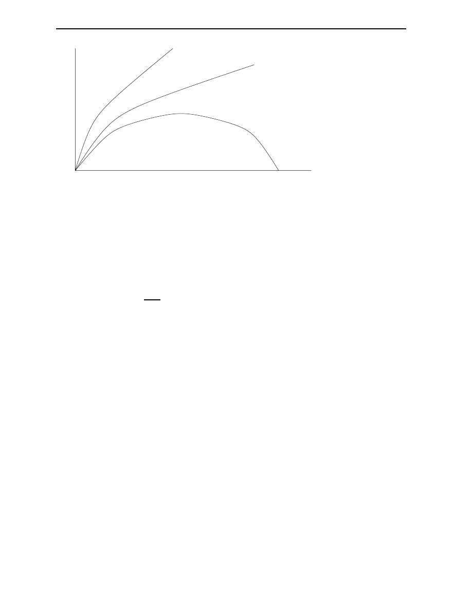
46
In the Beginning
R
O
T
k=+1
k=0
k=-1
Fig.
5.1:
Friedmann models
spacetime).
The Friedmann models predict three possible evolutions for the universe:
1.
Ever expanding universe (
k
=
;1
)
. The curvature in this model is equal to minus one.
The geometry is than said to be hyperbolic or open. The sum of the angles of a triangle is
for example less than 180 degrees. This model will describe the evolution of the universe if
the density of the universe is less than the critical density:
<
c
=
3
8
G
H
2
(5.1)
Where
G
is Newton's gravitational constant and
H
Hubble's constant. The combined mass
in the whole universe will be not enough to hold the expansion.
2.
Expansion holding at innity model (
k
=
0
)
. The geometry in this model is at or
Euclidean, the type we are familiar with and is used in Newtonian physics. The rate of
expansion will only slow down and will hold eectively at innity. The density must be
precisely equal to the critical density for this model to be valid.
3.
Closed universe (
k
=
1
)
. In this universe the geometry is spherical, e.g. the parallel lines
will diverge and the circumference of a circle will be smaller than
2
r
. The density is in
this case greater than the critical density, causing the universe to recontract.
The crucial fact that determines which Friedmann model accurately describes the evolution of the
universe is thus the current mass density. The distant future of the universe is directly dependent
upon it. Aside from the question how the expansion will proceed, there still remain paradoxes
unexplained by the Big Bang theory, to which we will turn now.
5.2 Initial conditions and ination
The laws of nature are generally based upon dierential equations. A set of dierential equations
xates the evolution of a system given the boundary conditions. The key equations in cosmology
are Einstein's equations of general relativity, and solving them without using very simple boundary

5.2 Initial conditions and ination
47
conditions is tremendously dicult. Besides this, the specication of initial conditions at the
actual initial singularity is non-trivial. If this initial state is timelike then some points of the initial
state will lie in the causal future of others. More probably, the initial state is spacelike and a
conventional boundary problem can be formulated which then requires the relevant variables to
be given on a spacelike hypersurface of constant cosmic time. This problem can be solved, in
principle, and its solution determines the present value of relevant cosmological variables like the
expansion rate, rotation, shear, curvature and density.
Now, the value of a set of cosmological invariants turns out to be responsible for the evolution
of the structure of the universe. It is the initial value (or more precisely, the value after a suitable
amount of time) of these variables that essentially constitutes the boundary condition of the
universe. A short description of each of them will therefore be given:
H
: Hubble's constant.
Describes the expansion rate of the universe. Mathematically dened
by:
_
R (t)
R (t)
(5.2)
Where
R
denotes the radius of the universe. In astronomy, Hubble's law states that the
velocity with which a galaxy (or star) is moving away from us is linearly dependent upon
the distance:
v
=
H
r
.
H
0
indicates the value of
H
today (about
75
25
kms
;1
Mpc
;1
).
: Flatness parameter.
The ratio of the density divided by the critical density, dened in the
previous section as the density which is just high enough to hold the expansion. A value
of one corresponds to a at universe with normal Euclidean geometry. If
is not precisely
one, but deviates from it slightly, then the value will diverge quite rapidly. This places
serious restrictions on the value it had in the early stages of the universe. For example, at
the Planck time the value must have been:
j
;
1j
10
;57
(5.3)
Finding an explanation for this ne-tuning of the initial condition is called the `atness'
problem.
: The cosmological constant.
The seen and unseen matter in the universe might not be
enough to produce a at universe [
k
=
0
]. This so-called `missing matter' problem inspired
some astronomers to revive the cosmological constant (cf. [22]). From the Friedmann
equation the following relation can be derived (assuming k=0):
+
3H
2
=
1
(5.4)
So, in order to get a at universe, a positive value of
may contribute to compensate
for the missing matter. Eectively, a positive cosmological constant acts as an antigravity
force, as it pushes galaxies away from another at very large distances, since the expansion
rate itself depends on the dierence between the density of matter (slowing the expansion)
and the cosmological constant (increasing the expansion rate). This should not be confused
with the dependence of geometry of the universe on the total energy density.
S
: The entropy per baryon.
The characteristic ratio of photons to baryons xes the entropy per
baryon and vice versa. An upper limit can be given by the requirement that the universe is
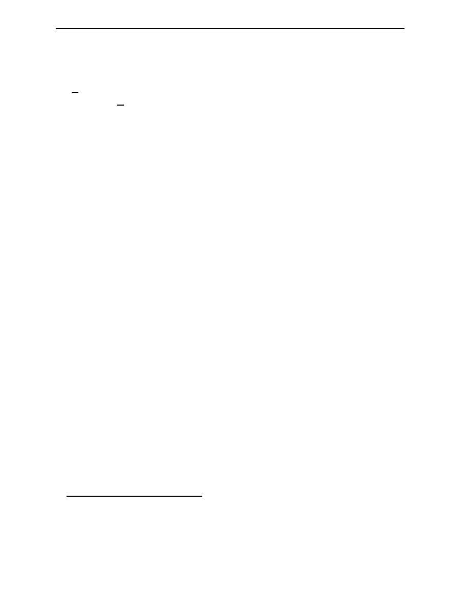
48
In the Beginning
not dominated by radiation today:
S
10
11
. It might be possible to derive a specic value
for this quantity from GUT's, in particular from the magnitude of CP-violation predicted by
such a theory.
: The density perturbations.
Anthropic arguments can give a precise range for this quantity:
10
;3
<
<
10
;4
. A slightly too high value would make the universe collapse before any
planetary system could have formed, and a slightly too low value would make the universe
expand beyond a rate which allows structures to evolve.
Especially the atness parameter and density perturbations seem to have `improbable' values.
Observation tells us that they lie within the narrow range given by anthropic arguments. This co-
incidence cries for an explanation. Was is an act of God or the result of an underlying mechanism?
Ination theory explores the latter possibility
3
.
After the Planck time, but still in the era of symmetry between the fundamental forces, some
exotic particles, the X and Y bosons, dominated the universe. Now, any particle can exist in
dierent phases, depending on the temperature. Water will be solid (ice) when cooled down, but
will be vapour beyond its boiling temperature. Similarly, the X and Y bosons can reside in certain
phases. If a change of phases occurs then dramatic events can ensue. The energy dierence
between two phases can accelerate the expansion of the universe for a nite period of time. This
can take place at speeds beyond the speed of light, since it is space itself that is expanding. This
period of expansion is called ination and can produce a series of remarkable consequences.
The particular shape of the ination potential, governing the interaction between the elds of
the particles, determines the succession of events and is largely dependent upon the temperature.
Since the elds will initially not be in a state where the potential is minimal, they will change
according to the shape of the potential. As the potential value of the elds changes, energy
is released and the universe expands exponentially. Eventually a minimum is reached and the
inationary period ends. As a result, ination attens the universe and
is pushed to one, while
at the same time irregularities get evened out. This explains the current value of
and the large
overall uniformity, even in regions not causally linked. Indeed, the distance over which causality
can correlate properties has been exponentially increased at an early moment. As noted before,
irregularities must not totally disappear since structures have evolved. Quantum uctuations of
the inated elds seem to have just the right magnitude to cause the right irregularities at the
end of ination, solving this problem too.
Ination theory seems to be a good candidate for explaining some of the magical coincidences
concerning the conditions shaping the Big Bang. It shows how a multitude of initial conditions
converge to roughly the same state at the end of ination. Additionally, the uniformity of regions
formerly supposed to be connected only at the initial singularity has been claried. Unfortunately,
recent observation show that there might be not enough mass to produce a at universe, and
without the introduction of a cosmological constant, ination theory will have to be adjusted (the
`bubble universes' variant seems to be a good candidate (cf. [4])). The atness parameter and
density perturbations being explained, there still remain three other quantities whose values are
not predicted in some grand scheme, but this problem seems to be less urgent. The origin of time
asymmetry, as caused the Big Bang, is deprived of some of its mystery.
3
See for example [25, 18] or [3, 6.12 and 6.13].

5.3 Another way out?
49
5.3 Another way out?
One might be disappointed by the explanation oered by ination theory to the question of
why the important cosmological variables have the values they have. What happened before the
inationary era? The energy densities in this stage of the history of the early universe require
a theory of quantum gravity for an accurate description. Nevertheless, some attempts have
been made and I will discuss two of them. The rst theory, Hawking's `no boundary condition',
will be described in some detail later, because it also has implications for the distant future of
the universe. It essentially seeks to dispense with the need of boundary conditions altogether
4
by studying the behavior of a `wave function of the universe' upon which certain (postulated)
restrictions are placed. The second theory is developed by Penrose and is based on a postulate
concerning the value of the Weyl curvature tensor of initial singularities, meaning `white holes',
like the Big Bang.
Penrose explores the consequences of placing a thermodynamic boundary condition on the
initial structure of the Big Bang (in [34] and [35]). This constraint consists of demanding that
the Weyl curvature tensor vanishes at initial singularities. The evolution of a universe placed
under this constraint is a very natural one, since the universe must necessarily expand away
from a virtually homogeneous and isotropic low entropy state, which a vanishing Weyl curvature
tensor implies, towards a state of higher entropy. The thermodynamic arrow of time is thus
explicitly inserted. If the universe is to evolve towards a second singularity, then this would be
a maximum entropy state, more disordered and totally dominated by the anisotropizing eect
of the Weyl curvature tensor. This picture could lead to a better understanding of the present
large scale structure of the universe, which is quiescence, isotropic and uniform in the midst of
all the dynamically more favorable degrees of freedom available for non-uniform expansion. His
motivation for this rather ad hoc solution of the problem of the initial condition of the universe is
largely based on the unlikeliness of the current situation. Virtually all other initial states lead to
universes where most matter is accumulated in black holes. In fact, the entropy of the state where
all matter is located in black holes is so huge that the initial state of our universe becomes highly
improbable, using Hawking's formula for the entropy of black holes and probability theory from
normal statistical mechanics. Penrose then argues that the alternative to his proposal, namely
assuming that the initial conditions came into existence by chance, is therefore very unlikely to
be true
5
. In my opinion, reasoning about a set of possible beginnings of the universe remains
problematic, since such a set does not exist. The likeliness of an event that happened only once is
undened if there is no set of events to choose from. If we do allow statements about the chance
of the current beginning to occur, then I still think that a law to the extent of restricting the
behavior of the Weyl curvature tensor to vanish only at initial singularities is a rather `expensive'
solution since a law normally generalizes some feature of a set of phenomena and there is only
4
An alternative attempt to show that the present structure of the universe is independent of the initial conditions
can be found in the `chaotic cosmology' program which tries to show that the universe, regardless its initial
state, becomes isotropic and homogeneous with the passage of time through the action of dissipative processes.
Unfortunately, this theory cannot be tested observationally since there is no way in telling the dierence between
a universe which began expanding isotropically with high thermal entropy and one which did not, but which later
underwent dissipative smoothing.
5
This is also an argument against the Strong Anthropic Principle which states that the universe must have those
properties which allow life to develop within it at some stage of its history. A much `cheaper' solution would be to
set up a small number of meticulously organized particle collisions to bring about the local life supporting entropy
uctuation we require than to produce it as a subset of a vastly bigger entropy uctuation the size of the entire
observable universe. We encountered a similar argument against Boltzmann's thesis.

50
In the Beginning
one initial singularity known: the Big Bang.
Alternatives to the two theories mentioned above are few. It can be reasoned that a causal
explanation requires accounting for something by reference to the existence and nature of other
objects and their features earlier in the history of the world. Such reference clearly becomes prob-
lematic in the case of the Big Bang. Another approach is the creation `ex nihilo' scenario where
a quantum uctuation is responsible for the beginning. Since time did not exist before this quan-
tum uctuation, there is `clearly enough time' available for it to occur in some grand background
reservoir. The apparent magnitude and scale on which it occurred may then be explained using
anthropic arguments, but such a line of reasoning does not appear to be very convincing to me.
Retracing the observed expansion back to its origin leads to a spacetime singularity. As we
go back into time the conventional Big Bang theory provides us with quite a convincing picture
of the ratio of light elements and the still observable background radiation. Still earlier in history,
inationary theory connects the apparently causally distinct regions and oers an explanation for
the high uniformity and atness of the universe, while it shows at the same time how a multiple
of initial conditions lead to the current state. Before the inationary era, arguments become
speculative, since a theory of quantum gravity is necessary but unavailable. Penrose's law and
Hawking's no boundary condition are the only serious theories available, but a true understanding
will probably only be possible within the context of a yet to nd theory quantum gravity. A sat-
isfying explanation for the initial conditions of the universe, ultimately responsible for the arrow
of time in cosmology, is thus still to be found. In the next chapter we will look how the arrow of
time emerges from Hawking's no boundary condition, and more generally at the fate the universe
awaits in the distant future, focusing on the second major issue of this part of the report.

Chapter
6
In the End
Besides a more detailed look at the origin of time asymmetry in the realm of quantum cosmology,
I will discuss time symmetric cosmologies in this chapter. One of the motivations for positing
a time symmetric cosmology is the possibility of a recontracting universe, in the distant future.
We will see how three arrows of time, viz. the psychological, thermodynamical and cosmological
are intimately connected in this event. Will the thermodynamical arrow of time reverse in this
`turn over' point in time? Arguments are various. The main question will be whether this event
is improbable or not. But rst I will return to the issue briey touched upon in the previous
chapter when initial conditions were discussed: quantum cosmology. A more detailed exposition
of quantum cosmology is necessary since it has important implications for time asymmetry, and
the correlation of the thermodynamical and cosmological arrow of time. It will be shown that
quantum cosmology in itself is not able to explain the strong thermodynamical arrow of time as it is
present today. Again, an appeal to boundary conditions will have to be made and the consistency
as well as the arguments for a particular choice of boundary conditions will be reviewed.
Throughout this chapter the notion of imposing a boundary condition at some end of the
evolution of the universe is important. If one does not assume a static or cyclic universe (a
universe trapped in ever lasting cycles of expansion and recontraction) then the universe has a
beginning and an end. The time ordering of these two events is not to be taken absolute here.
Three dierent evolutions for the universe are now possible: a universe evolving from a low entropy
initial state to a low entropy nal state, or one evolving from a low entropy to a high entropy end
(or vice versa), and nally one with two high entropy temporal ends. A generally accepted view
is that without imposing a boundary condition at one particular temporal end, the chance for the
universe to reside in a high entropy state is much higher than the chance to reside in a smooth,
low entropy state
1
. Time symmetrical cosmological theorists now argue that since the universe
was in a smooth state in the past, there is no reason not to apply such a boundary condition to
the nal singularity, given the fact that the laws of physics themselves are time symmetrical, and
time symmetrical boundary conditions are thus more `natural'. We will encounter this argument
later in this chapter in more detail.
Imposing a boundary condition at one end without specifying the state at the other end gives
rise to a strong thermodynamical arrow of time but does not, in itself, explain why the cosmological
and thermodynamical arrows should point in the same direction. This needs a separate argument
and I will show how each theory tries to accomplishes this.
1
Penrose estimated this chance to be 1 in
10
10
125
, based on the maximum entropy value realized when all matter
is accumulated in black holes, compared with the smooth conguration of the Big Bang.

52
In the End
6.1 Quantum cosmology
In the previous chapter the need for quantum cosmology for describing the universe in its very
early stages has been made clear. Beyond certain energies quantum gravitational eects will
be signicant. In order to establish a theory of quantum gravity one is forced to quantize the
fundamental equations of general relativity, the Einstein equations plus the evolution equations
for matter. This is by no means a trivial matter (see for example [14]). In the Dirac approach
one quantizes rst and later imposes the necessary constraints. This involves representing the
quantum state of the system by a wave functional
[h
ij
;
]
(where
h
ij
is a three metric and
a
scalar matter eld) which is a functional on superspace, the space of all three metrics and matter
elds. The classical constraints now translate into the Wheeler-DeWitt equation and momentum
constraints. Approximations will have to be made in order to solve these equations. One usually
restricts attention to a region of superspace in the immediate vicinity of homogeneity and this
involves going from superspace coordinates
(h
ij
;
)
to coordinates
(q
;
)
where
q
denote
a nite set of large homogeneous modes of the elds, known as minisuperspace modes, and
denote small inhomogeneous matter and gravitational perturbations about the homogeneous
modes which are retained only up to quadratic order in the Hamiltonian. The Wheeler-DeWitt
equation now takes on a new form in these coordinates. Only in the region where the wavefunction
satisfying these new equations, is oscillatory, the notion of classical spacetime is meaningful.
Solutions for the wavefunction then take on the form:
(q
;
)
=
C
(q
)e
iS
(q
)
(q
;
)
The phase
S
must satisfy a Hamilton-Jacobi equation and the matter mode or perturbation
wavefunction
must obey a Schrodinger equation. This is a Schrodinger equation along the
classical trajectories (possible histories of the universe) of the minisuperspace modes.
This formalism thus consists of equations which the wavefunction of the universe,
, must
satisfy. The wavefunction can essentially be regarded as a list of possible histories, classical or
otherwise, through which the universe could have evolved to its present quantum state, which
itself includes all logically possible particles and arrangements that could exist in the universe
at the present time (cf. [16]). To pick out a particular solution requires imposing boundary
conditions. Now, two such proposals for boundary conditions are known: the `tunneling' proposal
by Linde et al. [26] and the `no boundary' proposal by Hawking [19] . I will focus on the latter
and especially on its implications for time asymmetry.
The no boundary condition proposal of Hawking states that the quantum state of the universe
is determined by a path integral over positive denite metrics on closed spacetime manifolds. It
can only be used as a boundary condition by means of semi-classical approximations, and the path
integral which denes the quantum state is then evaluated using a saddle-point approximation.
The implications for the arrow of time follow from the behavior of perturbations of Friedmann
models of the universe, under the no boundary condition. At rst it was thought that when
the radius of the universe was small, the amplitude of the perturbations would be small and
thereby the entropy would be low. This then holds regardless in which phase (expanding or
recontracting) the universe is. Consequently, the thermodynamical arrow of time would reverse
when the universe would start recontracting. Later it was recognized that some saddlepoints
that were initially excluded in the evaluation of the path integral would instead contribute to the
value
2
. As a consequence, the correlation between the radius of the universe and amplitude of
2
Hawking admitted he made a mistake and adjusted his theory after taking knowledge of an article by Page [31]
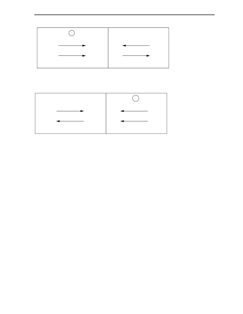
6.2 Time symmetric cosmologies
53
Big Bang
recontracting phase
cosmological arrow
thermodynamical arrow
Big Crunch
expanding phase
cosmological arrow
thermodynamical arrow
Disorder
Most disorder
Order
1
Fig.
6.1:
Arrows of time with an ordered Big Bang
Big Bang
recontracting phase
cosmological arrow
thermodynamical arrow
Big Crunch
Disorder
Most disorder
Order
expanding phase
cosmological arrow
thermodynamical arrow
2
Fig.
6.2:
Arrows of time with an disordered Big Bang
the perturbation would dier. Now large perturbations would probably exist at the end of the
recontracting phase and the thermodynamical arrow of time would not reverse.
Eectively, the no boundary condition thus predicts that the universe is smooth at one end of
time. It does not imply which particular end, the Big Bang or the Big Crunch is smooth. Why
then do we live in an expanding rather than recontracting universe? For there are two possible
situations where the cosmological and thermodynamical arrows of time agree in a universe with
one smooth end and one disordered temporal end. See gures 6.1 and 6.2. The rst step is to
argue that the psychological arrow of time and the thermodynamical arrow of time agree, since
information processing (occurring in the brain) costs entropy. Hawking now invokes the weak
anthropic principle to explain why situation 1 (cf. g. 6.1) rather than situation 2 (cf. g. 6.2)
should be a correct description of the current situation. Life could not survive the turnover in
the universe of situation 2, whereas it has yet to meet the turnover in the universe of situation
1. An observer would not be able to make the distinction between situations 1 and 2, since the
psychological and thermodynamical arrows point in the same direction. This concludes Hawking's
explanation why there is a boundary condition at (only) one end of time and why the resulting
arrows of time point in the direction in which the universe is expanding rather than contracting.
6.2 Time symmetric cosmologies
A statement made throughout this report is that the fundamental laws of physics are symmetric
with respect to time. A particular particle decay in nuclear physics is known to have dierent

54
In the End
decay rates in each direction of time, but it is generally accepted that this does not aect the
macroworld where the major arrows time manifest themselves. Besides this, there occurs only CP
violation and not CPT violation
3
, so by considering the decay rate of the anti-particle nothing
strange happens. Now, can the time symmetry of the fundamental laws somehow make the
thermodynamical and cosmological arrows agree in every phase of the universe? Some people
think it can, directly through the time symmetry of physical laws or indirectly through time
symmetrical boundary conditions. In the latter case a time symmetrical physics should imply that
the ultimate boundary conditions of the universe be time symmetrical, in the absence of a time
asymmetrical law implying otherwise. All arguments along these lines depend on the assumption
that an objective direction of time cannot be established.
A time symmetric cosmology subscribes to the idea that the entropy will decrease in the
recontracting phase of the universe, whether or not this actually takes place. The recontracting
phase then becomes a sort of mirror image of the expanding phase, restoring every change made
in the expanding phase. Since entropy is increasing now, in the expanding phase of the universe,
there must exist a `turning' point in time when the thermodynamical arrow reverses (or, less
strongly stated, a turnover in dierent regions at dierent times). Now, the major objection
against such a course of events is its supposed improbability. Would it not require an immense
ne-tuning of the (already improbable) initial conditions of the universe? I will return to this
question, after focusing on the supportive arguments for a time symmetric cosmology.
One of the rst formulations of a time symmetric cosmology can be found in an article by Gold
[13]. He argues that the entropy is low at both temporal ends of time. In this picture he connects
the various arrows of time in such a way that the arrow of thermodynamics depends upon the
arrow of radiation, which in itself depends upon the arrow of cosmology. The expansion of the
universe would allow the expansion of radiation by expanding the material between which the
radiation makes its way. Radiation in its turn aects thermodynamical systems by being a crucial
inuence from outside. The details of this process have been described here earlier. Gold realizes
that his viewpoint has some serious consequences. Should the reversal of the entropy gradient
not be extremely improbable and give rise to absurd events? People would rise from among the
dead, live their life remembering the future and die at birth. Radiation leaving our eyes would
converge on the surfaces of stars and heat them up. Gold does not seem to be troubled by these
pictures and replies [13, p. 409]:
\We should not belittle the monstrous degree of improbability that would seem to
be implied, but perhaps we should not think of it that way. Perhaps we should just
think of the universe as a four-dimensional map, the three space coordinates and one
time coordinate, in which the world lines of all particles are represented. Although the
pattern is enormously complex, it can be seen to be subject to certain well dened
rules. All these rules are independent of the sense in which the time coordinate is
labeled. These rules are the laws of physics. In addition it could be seen that the
pattern made by the lines fan out in one direction of the
t
coordinate or contracts in
the other. Nothing can be said about the probability or improbability of any part of
this pattern; it is just the pattern which is there. All that can be said is that: \If the
rules that underline the construction of the pattern are used in order to infer some
detail or knowledge of a limited region of the space and at one instant along the time
coordinate, then usually a much higher probability of making a correct guess exists
3
In quantum eld theory there exists a fundamental theorem, the CPT theorem, which states that a particle
remains unaected after inverting its charge (C), parity (P) and time (T) parameters.

6.2 Time symmetric cosmologies
55
when the region guessed at is on one side rather than the other side." \We remember
the past better than we remember the future."; or: \We can calculate the past more
accurately than we can calculate the future," these would be the only statements we
could make to distinguish the future and the past. With complicated systems the
dierence will be so great that it may appear to be a dierence in principle. The
asymmetry in the predictability is related to the actual pattern which certainly fans
out in one direction of
t
; it is in the boundary conditions and not in the laws."
Gold suggests here that the lawlike character of the Second Law exist only by our inability to
predict the future. The turning point and subsequent events should not be seen as improbable,
since for causality itself there is no place in this discussion. The laws of physics render all events
deterministic and probability is only a gment of our own mind. Not many supporters of time
symmetric cosmologies are prepared to go this far. We will see that other implementations and
arguments in favor of a time symmetric cosmology are possible.
Traditional arguments against time symmetric cosmologies can be found in Davies [7]. He rst
emphasizes that the recontraction of the universe, in a Friedmann model with
k
=
1
, does not
in itself cause the entropy to decrease. Instead, entropy will continue to increase throughout the
recontracting phase. Davies continues by stressing that a Loschmidt like reversal at the turning
point would place unnecessary further constraints on the initial condition. We will see however
that such a sharp turning point is not the only way to establish an eective reversal of the Second
Law. Especially the reversal of the emission of starlight, i.e. the reversal of the arrow of radiation,
seems to be a highly improbable event. A recontracting Friedmann universe only restores the
background radiation and not genuinely irreversible events like the emittance of radiation at the
surface of stars. He agrees that boundary conditions would have to be imposed at two instances
of time, which is hard to justify.
Penrose makes essentially the same point in [34] by stating that the expansion in itself is not
responsible for the entropy increase, but rather the initial smoothness. He further explores the
consequences of an actual reversal of the Second Law, and concludes that it leads to absurdities.
It runs as follows. Black holes are very similar to the nal Big Crunch and within the event horizon
the same physical conditions should apply. Now suppose that an astronaut enters the event horizon
of a suciently massive black hole, giving him enough time to conduct some experiments. Since
the Second Law is reversed, so is his (or her) psychological arrow of time. He would think he
is falling out of the black hole instead of entering it! Even a stranger situation arises when the
reversal of the Second Law does not happen suddenly at the event horizon, but gradually. An
observer would then start to remember the future (falling into the black hole) and would be able
to change his mind and decide not to cross the event horizon. This would eectively alter the
future he had already remembered. These absurdities lead Penrose to the conclusion that time
symmetrical cosmologies are no real possibilities.
Schulman [43] basically agrees with the main objection against time symmetric cosmologies
that the turning point, as it is generally depicted, is highly improbable. But he thinks that we
have the wrong image of what is actually happening. We should rst realize that `the natural
and automatic use of \arbitrary" or \controllable" initial conditions is already equivalent to the
setting of a thermodynamical arrow of time. For this reason, in discussing the arrow of time the
specication of system states should not be made at one particular time (\naturally" taken as the
initial time) but rather should be non-prejudicial, for example giving the boundary conditions at
two times.' After these initial remarks he investigates the behavior of a simple statistical system
restricted by two time symmetrical boundary conditions.

56
In the End
The consequence of two time boundary conditions on the behavior of statistical systems (for
example the evolution of the entropy) has been also studied by Cocke [5] and for example Gell-
Mann and Hartle [12]. The system most commonly used as an example is the Ehrenfest double
urn model, where randomly one of a set of numbered balls is switched between the two urns. A
double boundary condition is realized by demanding that there is a specic number of balls in
each urn at two instances of time. If these two boundary conditions are the same then one speaks
of time symmetric boundary conditions. Actual time symmetric evolution of the entropy is only
reached when a large set of evolutions satisfying the boundary conditions is averaged. Only then
does a turning point exist. Individual evolutions, on the other hand, can display time asymmetry.
A typical evolution depends on the relaxation time of the equilibrating processes. If the relaxation
time is short compared to the time interval between the two boundary conditions, equilibrium will
have been reached long before the magical turning point, at half the interval. A process with
a long relaxation time will never behave normally within the specic time and will consequently
not show any special behavior at the turning point. Processes with a relaxation time comparable
with the time interval itself are interesting because their behavior may indicate whether a nal
boundary condition exists. In the context of cosmology the dynamics of galaxies may thus provide
observational evidence for the existence of a nal singularity or Big Crunch.
Thus, the improbability of a turning point may be irrelevant, since such a sharp turning
point does not have to exist in a universe governed by two boundary conditions. Nevertheless,
arguments for the actual need for a nal low boundary condition are but few. At this point Price
oers an interesting view in his recent book [37, chapter 4]. He argues that, in the absence
of an objective direction of time, every argument to the eect that the initial conditions of the
universe were special can be turned into an argument with exactly the same implications for the
nal condition of the universe. So suppose that physics eventually nds an explanation for the
smooth initial state of the universe, then, since physics is generally time symmetrical, the nal
state should be alike. The alternative would be that the smooth initial state remains inexplicable.
In Price's opinion there is no real dierence in viewing the current universe as expanding from
a Big Bang or recontracting towards a Big Crunch. The improbability argument of the turning
point, according to Price, is irrelevant since it is a statistical and thus time symmetrical argument.
He also objects against a sharp turning point and favors what he calls a mixing model, where
structure or any piece of order is either the product of a singularity in one direction of time, or
the other. Each structure or region in space thus possesses a thermodynamic arrow of time of
its own. But how observers can distinguish between the origin of a particular `piece of structure'
and how a conict with determinism can be avoided remains unclear to me. Nevertheless, the
Archimedean viewpoint from nowhere shows which arguments to be suspicious of in explaining
the smoothness of the Big Bang.
We have now reviewed some arguments in favor of a universe governed by a boundary condition
in each direction of time. We saw how it was possible that an individual evolution can be time
asymmetrical although the boundary conditions are time symmetrical (allowing a diuse turning
point). Under these conditions the actual evolution of a system is not deterministic. State
transitions themselves may in general be described by a time symmetric law (as is the case with
the Ehrenfest double urn model), but during the evolution transition rates change, since the nal
condition must eventually be met. The laws of physics do not operate in this manner. Given a
particular state, the subsequent state is in principle determined. Actual individual evolutions in
the Ehrenfest double urn model are obtained by selecting evolutions, satisfying the nal boundary
conditions, from a large set generated from the initial state. Such an ensemble of universes
to choose from, in the cosmological case, does not exist. One can even doubt whether there

6.3 Conclusions
57
are cosmological two time boundary scenarios possible within the framework of a deterministic
physics. The highly specic initial smoothness may exclude a return to a low entropy state. In
this case, the nal boundary condition cannot be met physically.
6.3 Conclusions
Quantum cosmology in itself does not give rise to a specic arrow of time. The source of time
asymmetry must be sought in the boundary conditions. The no boundary condition turned out to
give rise to a strong thermodynamical arrow of time, which will not reverse in the recontracting
phase of the universe. Now, these conclusions are only valid under a number of approximations
(necessary in order to analyze any models in a quantized theory of general relativity). The models
in which Hawking proves that there exists a strong thermodynamic arrow of time under the no
boundary condition are theoretical models and their correctness is still to be proven observationally
(like ination theory).
The second part of this chapter focused on the plausibility of time symmetric cosmologies.
The consequences of consistently applying boundary conditions at both temporal ends of the
universe are interesting and cannot simply be dismissed as absurd or improbable, whether or not
the recontraction actually will take place. The most promising approach seems to be a time
symmetrical cosmology supporting a diuse turning point, with no sudden changes but a gradual
increase of events governed by a reverse thermodynamical arrow. There may even be observational
tests for this model since some processes have relaxation times on cosmic scales, and if a nal
boundary condition is present, it will inuence such processes to some extent. The actual presence
(or theoretical necessity) of a nal boundary condition remains a dicult issue. Price argues that
we only have to look back in time to see what a recontraction will look like, so the actual
presence of a future boundary condition is peripheral. Schulman appeals to the fundamental and
more natural character of time symmetric boundary conditions, while Gold points to the basic
time symmetry of physical laws themselves. Personally, these arguments do not convince me and
I argue that conicts with a deterministic physics cannot be excluded.


Chapter
7
Review and main conclusions
7.1 The Second Law
The Second Law arose as a phenomenological fact. Scientists have struggled ever since to place it
on a sound footing. Boltzmann pioneered in this eld by establishing the
H
-theorem. We saw how
he changed his mind after a number of serious objections were raised. In his hands, the Second Law
changed into a statistical truth: systems will most probably obey the Second Law, but exceptions,
although rare, may occur. The story does not end here. As statistical physics is very successful in
describing equilibrium systems, diculties remain when non-equilibrium phenomena are concerned.
And it is exactly in these phenomena that the arrow of time is observed. How then to `derive' an
arrow of time from the time symmetrical principles of statistical mechanics? Dynamical theories
developed to the end of predicting the time asymmetrical behavior of non-equilibrium phenomena
have been discussed. Somewhere in their foundation an asymmetrical principle must be invoked.
This may be applied in the form of an assumption about the transition rates of energy densities
or about the trajectory through phase space, but a so-called rerandomization posit, which is time
asymmetrical, must somehow be made. The fundamental asymmetry of this rerandomization
posit remains unexplained, unfortunately.
Two alternatives are available: interventionism from outside and explanations aiming to es-
tablish why only those initial conditions occur in nature which lead to entropy increasing behavior.
Both alternatives turn out not to be as satisfactory as hoped for if the parity of reasoning fallacy is
to be avoided. Why should the intervention from outside be time asymmetric to begin with? And
why should initial conditions be very special, this in contrast with the nal state of a system? In
fact, if one looks backwards in time the nal state is more special, since it leads to a low entropy
state, which is improbable. The branch system will be discussed below.
Contemporary discussions reect the current state of the issue: no widely accepted solution
has been found. Layzer explores a rather controversial route of deriving the thermodynamical
arrow of time from cosmological principles. Coveney and Higheld think the only solution is to
resort to placing the Second Law on equal footing with the fundamental laws of physics, since
the thermodynamical arrow of time is obviously present, and crucial for self-organizing systems.
Price favors the view from nowhen and criticises many orthodox explanations of the arrow of
time. However, his time symmetrical worldview does not oer any solutions for the existence of
the Second Law, for he seems to favor the branch system mechanism with which there are serious
problems, in my opinion.
Now, is there a solution to the problem of the time asymmetry of the Second Law? This

60
Review and main conclusions
question is dicult to answer. Dierent people have dierent notions of what actually counts as
a solution. In this paper I have searched for a derivation of the asymmetry starting from grounds,
assumptions, laws or principles that are uncontested. I have made the concepts and language of
several theories and the theories themselves clear, or at least I have attempted to do so. The
ultimate theory has not been found, of course. The most promising approach, assuming a low
entropy Big Bang, time symmetrical physical laws, and a branch system mechanism, has been
discussed to the extent of how the low entropy source can explain the parallelism and entropy
gradient of branch systems, that is, the connection between the cosmological and thermodynamical
arrow of time. Nevertheless, many insights have been reviewed and the overall picture has become
clearer, I hope. From interventionism to the atemporal viewpoint, and from coarse-graining
entropy to the strong cosmological principle, many issues have been presented.
The existence of irreversible phenomena is an irrefutable fact. Whether their explanation is
ultimately statistical or dynamical in nature, it still calls for a satisfactory explanation. If one
does not accept that a time asymmetrical principle must somehow be incorporated into a theory
predicting the evolution of a thermodynamical system, then the last resort for introducing time
asymmetry must be found in the initial conditions. The spin-echo experiment supports this point
of view. Why then do only those initial conditions occur that lead to time asymmetrical behavior
in branch systems? At this point, all explanations seem to fail in one or more respects. From
the overly simplistic account of Price to the highly mathematical arguments of Prigogine, all
explanations seem to have their weaknesses. Even to take it as a fact that only those initial
conditions occur that lead to time asymmetrical behavior, does not solve all problems, because
the existence of a low entropy Big Bang, the ultimate source of all branch systems, is in need
of an explanation. In my opinion, the relation between the cosmological arrow of time and the
thermodynamical arrow of time is by no means a settled issue. Maybe the Second Law itself is
more fundamental than other laws of physics, or should be postulated as being on an equal footing
with classical mechanics. As long as a grounding theory has not been found, such possibilities
should not be excluded, despite their ad hoc nature.
7.2 Cosmology
The second part continued with the most promising lead obtained in the rst part, namely the
approach of explaining time asymmetry in thermodynamical systems by means of the branch
system mechanism. This mechanism can at least explain how a low entropy source can x an
entropy gradient, but how the parallelism between a large set of systems is to arise remains a
dicult point. We saw how the source of negentropy in local thermodynamical systems ultimately
depends on a smooth Big Bang. Other explanations for the current low entropy state (the
Boltzmann hypothesis and steady state theory) turned out to be unconvincing, for they lacked
any account for the observation of microwave background radiation and the ratio of light elements.
The origin of a smooth Big Bang has been extensively discussed. It plays a crucial role in
the two major issues which were investigated in the second part of this report: how to explain
the low entropy early condition of the universe and the question whether the cosmological and
thermodynamical arrows will be aligned in every phase of the universe.
Insight into the rst issue requires some knowledge of the Big Bang. It turned out that
classical Big Bang theory oers an explanatory ground for some crucial cosmological observations
but breaks down at high energies. We have to go further back in time to resolve our rst issue.
After an exposition of the important quantities that determine the evolution of the structure of

7.2 Cosmology
61
the universe, a theory oering a plausible explanation for the size of some of these quantities
(the atness and size of local irregularities) was discussed. As alternatives are few, maybe only
Penrose's suggestion to postulate a new law precisely to this end is to be taken seriously. Ination
theory proved to be quite consistent and convincing but will have to be reformulated if the universe
turns out not to be at after all.
The search for time asymmetry does not end with inationary theory since one must account
for the conditions giving rise to an inationary expansion of the universe. Going further back into
time, it is quantum cosmology that describes the universe. Although a bit speculative due to
the severe diculties one encounters in creating a quantum theory of gravity, equations for the
wavefunction of the universe can be derived. And again, quantum cosmology itself does not give
rise to an arrow of time, as this will depend upon the boundary conditions. Hawking's no boundary
condition is the most commonly known proposal and it implies that one end of the universe is
smooth. The other end will most probably be typical and thus of high entropy. The weak anthropic
principle is now invoked to explain why we nd ourselves in an expanding universe: life could not
survive the turnover in the universe congured according to other possibility. Nevertheless, if life
survived the turnover, only the objective direction of time would dier since the psychological and
thermodynamical arrows of time point in the same direction and observers would still claim they
live in an expanding universe.
The next major issue, whether the cosmological and thermodynamical arrows of time will
always point in the same direction, is most relevant in time symmetric cosmologies, which state
that the two arrows will be aligned in every phase of the history of the universe. Arguments
against and in favor of this point of view have been discussed. At the supportive side we nd
Gold, reasoning consequently from the fact of the symmetry of physical laws towards a world view
in which probability or causality have no place. A sharp turning point between the expanding
and recontracting phases should therefore not be considered improbable, which is the major
objection against time symmetric cosmologies, as pointed out by Davies or Penrose. A viewpoint
not demanding an exact time symmetrical behavior of the universe with respect to the turning
point, is advanced by Schulman and Cocke, and in a slightly dierent formulation by Price, in his
mixing model. Arguments for the actual existence of a nal boundary condition seem somewhat
less convincing. A simple statistical model is used to show that time symmetrical laws can
produce an evolution satisfying two time symmetrical boundary conditions. Yet time symmetry
is only reached when a large set of evolutions is averaged, and my major concern is whether a
deterministic physics can support an evolution satisfying time symmetrical boundary conditions
in the cosmological case.
Almost all views expressed by the various authors lack the possibility of performing an ob-
servational test. Whether or not the arrow of time of thermodynamics will reverse or not will
remain a theoretical debate, where the consistency and the power of persuasion counts. However,
current observational evidence indicate that the universe is not at and will not contain enough
matter to hold the expansion. Heat death will be inevitable. Scenarios envisaging people rising
from among the dead and scattered structures being restored to order will remain the exclusive
domain of science ction.

62
Review and main conclusions
7.3 Main Conclusions
1. A convincing derivation of the time asymmetric Second Law from time symmetric funda-
mental laws has not been devised so far.
2. The common `initial' conditions of all branch systems cannot explain their parallelism, i.e.
their common entropy gradient. One would have to distinguish their creation from their
reabsorption on other grounds, viz. an objective direction of time, which is not available.
3. Time symmetrical statistical physics cannot predict the evolution of a thermodynamical
system, if an objective direction of time is not given, since it can be overridden by boundary
conditions, in which case a system does not always evolve to a more probable state.
4. Ination theory oers the best explanation for a smooth Big Bang so far.
5. Quantum cosmology itself does not explain the strong thermodynamical arrow of time,
without resorting to boundary conditions.
6. The no boundary condition proposal seems to be the best proposal available in explaining
the arrow of time in cosmology and its present alignment with the thermodynamical arrow
of time.
7. The theoretical necessity of a nal boundary condition is independent of the time symmetry
of physical laws.
8. The probability of the initial state of the universe or its turning point remains a problematic
issue since there is no set of universes to choose from.
9. Time symmetric cosmologies that support a diuse turning point are more favorable than
those which do not.

Glossary of technical terms
I do not claim to present a complete list of technical terms. Every reader will already know some
concepts presented here and may not understand others that I have not included in my list, but
this glossary aims at oering some help for the less technically educated reader.
Background radiation.
The radiation still existing as an afterglow of the decoupling of radiation
and matter, is called the microwave background radiation, and provides a snapshot of the
universe when it was seven hundred thousand years old.
Big Bang.
The Big Bang theory subscribes the view that all matter and radiation (actually
spacetime itself) originated from a spacetime singularity back in time.
Big Crunch.
If the universe recontracts again in the distant future, then this event is called the
Big Crunch.
Black Hole.
A black hole is a state of matter with such a high density that even light cannot
escape. Beyond the event horizon, surrounding a black hole, nothing can escape from falling
in.
Concentration curve.
This curve describes the average behavior of representative points satis-
fying one macrostate. In general, the curve will approach the equilibrium value.
Cosmological constant.
This constant appears in a term added by Einstein to his eld equations.
Such a term would produce a repulsion at very large distances, and would be needed in a
static universe to balance the attraction due to gravitation.
Curvature of space.
Curvature of space is caused by the distribution of mass and aects the
distances and angles over which bodies will move through space. A at universe is governed
by normal Euclidean geometry, in contrast with a closed or open universe.
Ensemble.
An ensemble is a set of mental copies of one thermodynamical system satisfying one
macrostate and dierent microstates.
Entropy.
Entropy is a measure (depending on the particular denition) for the degree of chaos
in a system.
Ergodicity.
The feature of ergodicity guarantees that the phase space average and the time
average of a phase function are equal. The rst denition of ergodicity required that the
trajectory of the representative point of a system would eventually pass through every point
in phase space, but when it became known that no single system could comply with this
denition it was replaced by the quasi-ergodic hypothesis. This in its turn was replaced by
metric indecomposibility.
Equations of motion.
These equations constitute a set of dierential equations xing the dy-
namic behavior of a system.

64
Glossary of technical terms
Equilibrium.
A system is in equilibrium when the macroscopic variables do not change.
Evolution, trajectory.
The evolution of a system is its time development in space.
Fine-grained entropy.
Fine-grained entropy is a denition of entropy where one assumes no
partitioning of phase space, in contrast with coarse-grained entropy.
Friedmann model.
The Friedmann models are cosmological models describing the evolution of
the universe, based on general relativity and the Cosmological Principle.
H
-theorem .
This theorem states that the
H
-value (eectively minus the entropy) will mono-
tonically decrease.
Inationary theory.
According to inationary theory, the early universe went through a period
of exponential expansion, during which space was attened out and global irregularities
disappeared. Local irregularities, necessary for structures to emerge, were present due to
quantum uctuations.
Initial conditions.
The initial conditions form set of variables specifying the state of the system
at the initial instant of time.
Kinetic equation.
This equation describes the time evolution of macroscopic observables, in the
sense of a `concentration curve' of an ensemble evolution.
Liouville's theorem.
This theorem states that ne-grained entropy will remain constant.
Macroscopic information.
This information reects our knowledge of the statistical properties
of a system.
Macrostate.
The macrostate comprises the set of macroscopic variables which the state of a
system.
Microscopic information.
This information reects our knowledge of correlations between prop-
erties of individual particles.
Microstate.
The microstate comprises the set of coordinates and velocities of each of all the
particles.
Molecular chaos.
Molecular chaos exists when particles are uncorrelated before they collide.
Non-equilibrium.
A system in non-equilibrium resides in an unstable state and will therefore
change macroscopically.
Phase space.
Phase space is an abstract space wherein a system of
N
particles can be repre-
sented by
N
points, as in
-space, or by one point, as in
;
-space. If a whole system is
represented by one point then this point is called the representative point.
Planck Time.
The very short time interval which can be `made' from the fundamental constants
relevant in cosmology is called the Planck Time.
Recurrence objection.
This objection against the
H
-theorem states that a system must even-
tually return to any state in which is has been in its time evolution, according to Poincare's
recurrence theorem. As a consequence a thermodynamic system initially in non-equilibrium
must return to this state and cannot show a monotonic approach to equilibrium in the
innite time limit.
Quantum gravity (cosmology).
Beyond a certain energy density quantum mechanical eects
will become important, and general relativity will have to be quantized. A theory in suc-
ceeding this would be a theory of quantum gravity.

Glossary of technical terms
65
Rerandomization.
Rerandomization is the process of the removal of some particular micro-
correlations in the current state.
Reversibility objection.
Another objection against the
H
-theorem points to the fact that the
time-reversed state of a system must evolve back to its original state, allowing anti-
thermodynamic behavior to occur.
Strong anthropic principle.
This principle states that the universe must have those properties
which allow life to develop within it at some stage of its history.
Strong cosmological principle.
This principle states that the spatial distribution of matter in
the universe is homogeneous and isotropic, apart from local irregularities, which themselves
are statistically homogeneous and isotropic.
Two time boundary conditions.
If the state of the system is xed at two distinct time instants
then it is said to be governed by two time boundary conditions. It has been emphasized
that this does not imply the evolution in between to be time symmetrical, if the boundary
conditions are time symmetrical.
Wave function of the universe.
This wave function can essentially be regarded as a list of
possible histories, classical or otherwise, through which the universe could have evolved to its
present quantum state, which itself includes all logically possible particles and arrangements
that could exist in the universe at the present time.
Weak anthropic principle.
This principle states that the observed values of all physical and
cosmological quantities are not equally probable but take on values restricted by the re-
quirement that there exist sites where carbon-based life can evolve and by the requirement
that the universe be old enough for it to already have done so.


References
[1] V. I. Arnold and A. Avez. Ergodic problems in classical mechanics. Benjamin Inc., New
York, 1968.
[2] P. W. Atkins. Time and dispersal: the second law. In R. Flood and M. Lockwood, editors,
The Nature of Time. Basil Blackwell Ltd., Oxford, 1986.
[3] J. D. Barrow and F. J. Tipler. The anthropic cosmological principle. Oxford University Press,
Oxford, 1986.
[4] M. A. Bucher and D. N. Spergel. Ination in a low density universe. Scientic American,
280(1):42{49, jan 1999.
[5] W. J. Cocke. Statistical time symmetry and two-time boundary conditions in physics and
cosmology. Phys. Rev., 160(5):1165{1170, 1967.
[6] P. Coveney and R. Higheld. The Arrow of Time. Flamingo, London, 1990.
[7] P. C. W. Davies. The Physics of Time Asymmetry. Surrey University Press, London, 1977.
[8] R. D'Inverno. Introducing Einstein's Relativity. Clarendon Press, Oxford, 1992.
[9] J. Earman and J. D. Norton. Exorcist xiv: The wrath of Maxwell's demon. Stud. Hist. Phil.
Mod. Phys., 29(4):435{471, 1998.
[10] J. P. Eckmann and D. Ruelle. Ergodic theory and strange attractors. Rev. Mod. Phys.,
57:617{656, 1985.
[11] P. Ehrenfest and T. Ehrenfest. The conceptual foundations of the statistical approach in
mechanics. Dover Publications, New York, 1990. First published in German in 1912.
[12] M. Gell-Mann and J. B. Hartle. Time symmetry and asymmetry in quantum mechanics and
quantum cosmology. In J. J. Halliwell, J. Perez-Mercader, and W. H. Zurek, editors, Physical
Origins of Time Asymmetry. Cambridge University, 1994.
[13] T. Gold. Arrow of time. Amer. J. Phys., 30:403{410, 1962.
[14] J. J. Halliwell. Quantum cosmology. In J. J. Halliwell, J. Perez-Mercader, and W. H. Zurek,
editors, Physical Origins of Time Asymmetry. Cambridge University, 1994.
[15] J. J. Halliwell and S. W. Hawking. Origin of structure in the universe. Phys. Rev. D,
31(8):1777{1791, 1985.

68
References
[16] J. B. Hartle and S. W. Hawking. Wave function of the universe. Phys. Rev. D, 28(12):2960{
2975, 1983.
[17] S. W. Hawking. Arrow of time in cosmology. Phys. Rev. D, 32(10):2489{2495, 1985.
[18] S. W. Hawking. A brief history of time. Bantan Books, 1988.
[19] S. W. Hawking. The no boundary condition and the arrow of time. In J. J. Halliwell,
J. Perez-Mercader, and W. H. Zurek, editors, Physical Origins of Time Asymmetry. Cam-
bridge University Press, 1994.
[20] S. W. Hawking, R. Laamme, and G. W. Lyons. Origin of time asymmetry. Phys. Rev. D,
47(12):5342{5355, 1993.
[21] A. Khinchin. Mathematical foundations of statistical mechanics. Dover Publications, New
York, 1949.
[22] L. M. Krauss. Cosmological antigravity. Scientic American, 280(1):34{41, jan 1999.
[23] N. Krylov. Works on the foundations of statistical physics. Princeton University Press, 1979.
[24] R. Laamme. The arrow of time and the no boundary proposal. In J. J. Halliwell, J. Perez-
Mercader, and W. H. Zurek, editors, Physical Origins of Time Asymmetry. Cambridge Uni-
versity Press, 1994.
[25] D. Layzer. The arrow of time. Scientic American, 233(6):56{69.
[26] A. D. Linde. Quantum creation of inationary universe. Il Nuovo Cimento, 39:401, 1984.
[27] A. D. Linde. The self-reproducing inationary universe. Scientic American quarterly,
9(1):98{105, 1998.
[28] F. Mandl. Statistical physics. Wiley, New York, second edition, 1988.
[29] J. D. North. The measure of the universe. Clarendon Press, Oxford, 1965.
[30] O. E. Overseth. Experiments in time reversal. Scientic American, pages 89{101, oct 1969.
[31] D. N. Page. Will entropy decrease if the universe recollapses? Phys. Rev. D, 32(10):2496{
2499, 1985.
[32] O. Penrose and J. L. Lebowitz. Modern ergodic theory. Phys. Today, pages 23{29, feb 1979.
[33] O. Penrose and I. C. Percival. The direction of time. Proc. Phys. Soc., 79:605{616, 1962.
[34] R. Penrose. Singularities and time-asymmetries. In S. W. Hawking and W. Israel, editors,
General relativy, An Einstein Centenary Survey. Cambridge University Press, 1979.
[35] R. Penrose. The Emperor's New Mind. Oxford University Press, Oxford, 1989.
[36] K. Popper. Time's arrow and entropy. Nature, 207:233{234, jul 1965.
[37] H. Price. Time's Arrow and Archimedes' Point. Oxford University Press, Oxford, 1996.
[38] I. Prigogine and I. Stengers. Order out of Chaos. Bantam Books, New York, 1984.

References
69
[39] H. Reichenbach. The Direction of Time. University of California Press, 1956.
[40] T. M. Ridderbos. A point outside time? Stud. Hist. Phil. Mod. Phys., 28B(4):523{535,
1997.
[41] T. M. Ridderbos and M. L. G. Redhead. The spin-echo experiments and the second law of
thermodynamics. Found. of Phys., 28(8):1237{1270, 1998.
[42] S. F. Savitt. Time's Arrows Today. Cambridge University Press, Cambridge, 1995.
[43] L. S. Schulman. Time-symmetric cosmology and denite quantum measurement. In J. J.
Halliwell, J. Perez-Mercader, and W. H. Zurek, editors, Physical Origins of Time Asymmetry.
Cambridge University Press, 1994.
[44] L. Sklar. Physics and Chance: Philosophical issues in the foundations of statistical mechanics.
Cambridge University Press, 1993.
[45] S. Weinberg. The First Three Minutes. Basic Books Inc., New York, 1977.
[46] H. D. Zeh. The Physical basis of the direction of time. Springer-Verlag, Berlin, 1989.
[47] Ya B. Zel'dovich. Cosmology and the early universe. In S. W. Hawking and W. Israel, editors,
General relativy, An Einstein Centenary Survey. Cambridge University Press, 1979.
Wyszukiwarka
Podobne podstrony:
The Role of Vitamin A in Prevention and Corrective Treatments
The Structure of DP in English and Polish (MA)
The Problem Of Order In Society, And The Program Of An Analytical Sociology Talcott Parsons,
The Spectre of Shakespeare in Rosencrantz and Guildenstern are Dead
The Language of Architecture in English and in Polish Jacek Rachfał
Guide to the properties and uses of detergents in biology and biochemistry
Political Thought of the Age of Enlightenment in France Voltaire, Diderot, Rousseau and Montesquieu
A Comparison of the Status of Women in Classical Athens and E
Industry and the?fects of climate in Italy
The?ll of Germany in World War I and the Treaty of Versail
Pride and Prejudice The Theme of Pride in the Novel
Mussolini's Seizure of Power and the Rise of?scism in Ital
Guide to the properties and uses of detergents in biology and biochemistry
Jakobsson, The Peace of God in Iceland in the 12th and 13th centuries
prepositions of time on at and in 2 brb29
RADIOACTIVE CONTAMINATED WATER LEAKS UPDATE FROM THE EMBASSY OF SWITZERLAND IN JAPAN SCIENCE AND TEC
więcej podobnych podstron