3
A manual for the design, balancing and troubleshooting
of hydronic radiator heating systems.
BALANCING OF
RADIATOR SYSTEMS
TA-Handbok 3 (GB) 03-04-24 14.25 Sida 1
“Balancing of radiator systems” is the third manual in the TA series of publications about hydronic design and balan-
cing. The first manual deals with balancing control loops, the second with balancing distribution systems and the
fourth with hydronic balancing with differential pressure controllers.
This publication has been prepared for an international audience. Because the use of language and terminology differs
from country to country, you may find that some terms and symbols are not those you are used to. We hope this will
not cause too much inconvenience.
Written by Robert Petitjean. Warm thanks to TA experts in hydronic balancing: Bjarne Andreassen, Eric Bernadou,
Jean-Christophe Carette, Bo G Eriksson and Peter Rees for their valuable contributions.
Production: Sandberg Trygg AB, Sweden.
— 3rd edition —
Copyright 2002 by Tour & Andersson AB, Ljung, Sweden. All rights reserved. No part of this book may be
reproduced in any form or by any means without permission in writing from Tour & Andersson AB. Printed in
Sweden, April 2003.
Opera House, Gothenburg, Sweden
TA-Handbok 3 (GB) 03-04-24 14.25 Sida 2

Contents
Why balance?
......................................................................................................................................... 5
1- Balancing of radiator systems
...................................................................................................... 7
1.1-
Overflows cause underflows ..................................................................................................... 7
1.2-
Overflows in distribution .............................................................................................................. 9
2- Radiator valves
............................................................................................................................... 11
2.1- General
...................................................................................................................................... 11
2.1.1-
When the inlet valve is used only to isolate
2.1.2-
When the inlet valve is used to isolate and adjust the flow
2.2-
What is a thermostatic valve? ................................................................................................ 12
2.3-
Thermostatic valves and the supply water temperature .................................................... 13
2.4-
Is the thermostatic valve a proportional controller? ........................................................... 14
2.5-
Should a plant be hydraulically balanced with all thermostatic valves fully open? ........ 17
2.6-
Accuracy to be obtained on the flow ...................................................................................... 18
3- Radiators
.......................................................................................................................................... 20
3.1-
Nominal and design conditions .............................................................................................. 20
3.2-
Selection of a radiator not working in nominal conditions ................................................ 20
3.3-
Emission of a radiator as a function of the water flow ....................................................... 21
3.4-
Selection of the design water temperature drop ................................................................... 22
3.5-
Existing plants........................................................................................................................... 23
4- Two-pipe distribution
.................................................................................................................. 24
4.1-
Balancing of radiators based on a constant
∆
p .................................................................... 24
4.1.1-
Choosing the design differential pressure
4.1.2-
Presetting the thermostatic valve
4.1.3-
Non-presettable thermostatic valves
4.1.4-
Limitations of choice with the same
∆
p for all radiators
4.2-
Presetting based on calculated
∆
p ......................................................................................... 29
B A L A N C I N G O F R A D I A T O R S Y S T E M S
3
TA-Handbok 3 (GB) 03-04-24 14.25 Sida 3

4
4.3-
Constant or variable primary flow......................................................................................... 30
4.3.1- About
noise
4.3.2-
Constant primary flow
4.3.2.1- A bypass and a secondary pump minimise the
∆
p on the branch
4.3.2.2- A BPV stabilises the
∆
p on the branch.
4.3.3-
Variable primary flow
4.3.3.1- A plant with balancing valves
4.3.3.2- A
∆
p controller keeps the
∆
p constant across a branch
5- One-pipe distribution
................................................................................................................... 39
5.1- General
...................................................................................................................................... 39
5.1.1- Advantages
5.1.2-
Disadvantages and limitations
5.1.3-
Emission from pipes
5.2- One-pipe
valves
........................................................................................................................ 44
5.2.1-
Constant bypass – variable Kv
5.2.2-
Variable bypass – constant Kv
5.2.3-
Protection against double circulation
5.3-
Proportion of the loop flow in the radiator (
λ
coefficient) ................................................. 45
5.3.1-
50% flow in the radiator (
λ
= 0.5)
5.3.2-
Choice of another flow in the radiator
5.4-
The loop flow ............................................................................................................................ 47
5.4.1-
Based on a given
∆
T
5.4.2-
Based on the largest radiator in the loop
5.4.3-
Final choice of the loop flow
5.5-
Pressure losses in the loop ....................................................................................................... 48
Appendices
A-
Calculation of radiators in several conditions ...................................................................... 49
B-
Pressure losses in pipes ........................................................................................................... 52
Further information is available in our general book on balancing “Total hydronic balancing”.
B A L A N C I N G O F R A D I A T O R S Y S T E M S
TA-Handbok 3 (GB) 03-04-24 14.25 Sida 4

Why balance?
Many property managers spend fortunes dealing with complaints about the indoor climate.
This may be the case even in new buildings using the most recent control technology.
These problems are widespread:
• Some rooms never reach the desired temperatures.
• Room temperatures oscillate, particularly at low and medium loads, even though the
terminals have sophisticated controllers.
• Although the rated power of the production units may be sufficient, design power can’t
be transmitted, particularly during start-up after weekend or night setback.
These problems frequently occur because incorrect flows keep controllers from doing
their job. Controllers can control efficiently only if design flows prevail in the plant
when operating at design condition.
The only way to get design flows when required is to balance the plant. Balancing
means adjusting the flows at correct values at design condition. Avoiding underflows at
design condition makes sure that underflows will be avoided in all other normal conditions.
Balancing is necessary for three reasons:
1. The production units must be balanced to obtain design flow in each boiler or chiller.
Furthermore, in most cases, the flow in each unit has to be kept constant when required.
Fluctuations reduce the production efficiency, shorten the life of the production units
and make effective control difficult.
2. The distribution system must be balanced to make sure all terminals can receive at
least design flow, regardless of the total average load on the plant.
3. The control loops must be balanced to bring about the proper working conditions for
the control valves and to make primary and secondary flows compatible.
This manual deals with the balancing of radiator distribution systems.
Other manuals available are:
Manual 1: Balancing of control loops.
Manual 2: Balancing of distribution systems.
Manual 4: Balancing with differential pressure controllers.
B A L A N C I N G O F R A D I A T O R S Y S T E M S
5
TA-Handbok 3 (GB) 03-04-24 14.25 Sida 5
Why is the average temperature higher in a plant that is not balanced? During cold weather it
would be too hot close to the boiler and too cold on the top floors. People would increase the
supply temperature in the building. People on the top floors would stop complaning and people
close to the boiler would open the windows. During hot weather the same applies. It is just that it
would be too cold close to the chiller, and too hot on the top floors. One degree more or less in a
single room rarely makes any difference to human comfort or to energy costs. But when the average
temperature in the building is wrong, it becomes costly.
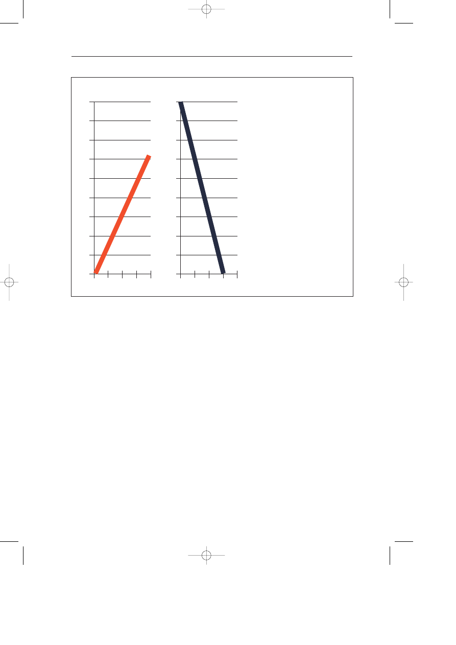
One degree above 20 °C increases heating costs by at least 8 per cent in mid Europe (12 per
cent in the south of Europe). One degree below 23 °C increases cooling costs by 15 per cent in
Europe.
B A L A N C I N G O F R A D I A T O R S Y S T E M S
6
%
45
35
25
15
5
20
21
22
23
˚C
35
25
15
5
20
21
22
23
˚C
%
45
Percentage increase in
energy costs for every
degree C too high, or too
low, relative to average
building temperature.
Cooling
Heating
TA-Handbok 3 (GB) 03-04-24 14.25 Sida 6
1 . B A L A N C I N G O F R A D I A T O R S Y S T E M S
7
1. Balancing of radiator systems
1.1 Overflows cause underflows
The design flow must pass through each radiator at design condition,
which requires individual local adjustment.
At first sight, there would appear to be no advantage in balancing a heating plant
equipped with thermostatic valves as their function is to adjust the flow to the correct
value. Hydronic balancing should therefore be obtained automatically.
This would be more or less true in normal operation provided that all control loops
are stable. However, unbalanced radiators create major distortions between flows. Let us
consider two radiators on the same branch, one 500 W and the other 2500 W. The installer
usually installs the same thermostatic valves on all radiators. The radiator headloss is
normally negligible and the flow is limited mainly by the thermostatic valve. Flows will
therefore be the same for both radiators. If this flow is right for the 2500 W radiator, it is
five times the design value for the 500 W radiator.
As if that were not enough to create problems in a plant, other distortions are added.
For example, thermostatic valves left at the maximum set point, will keep them open
permanently. If the maximum flow is not limited, these overflows create underflows in
other parts of the plant where the required room temperature cannot be obtained.
Restarting the plant, every morning after night setback, is a serious problem as
most thermostatic valves are open. This creates overflows getting unpredicted pressure
drops in some pipes, consequently reducing the flows in unfavoured circuits. These circuits
do not receive sufficient water until the favoured thermostatic valves are at their nominal
lift. This causes the plant to have a non uniform start-up, which makes management by a
central controller difficult and also makes any form of optimisation practically impossible.
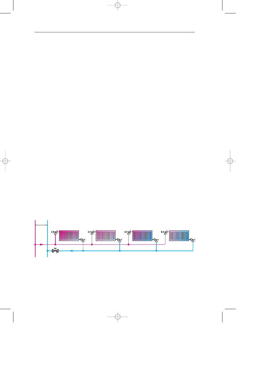
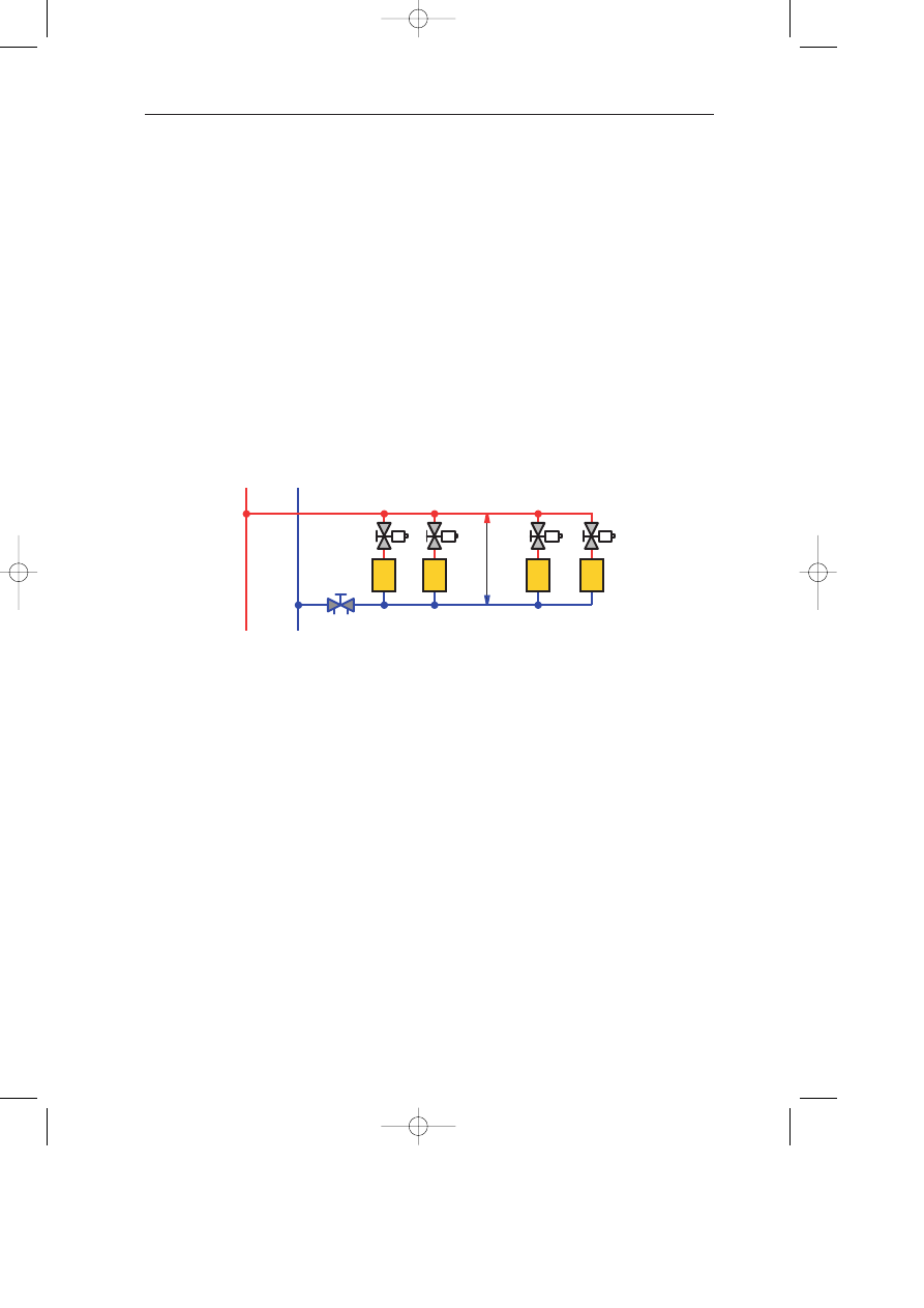
Figure 1.1 represents a branch with four radiators. The pressure drops in the pipes
between each radiator are one kPa at design flow. The available differential pressure is
9 kPa for the first radiator and 6 kPa for the last one.
The presettings of the thermostatic valves have been chosen to obtain the design flow in
each radiator. The branches and risers are also balanced.
Fig 1.1. Branch with four radiators.
30 kPa
80
°
C
1
2
3
4
TA-Handbok 3 (GB) 03-04-24 14.25 Sida 7
The results are in table 1.1.
Now, let us consider the case of a plant where the risers and branches are balanced, but
the radiator valves are not preset. The total flow in the branch is correct, but the radiators
are not working at design flow. The results are shown in table 1.2.
The first radiator receives 6 times its design flow. This increases the heat output by only
14%. That means that the necessary time to reach the design room temperature, after a
night setback, is not reduced significantly. If the thermostatic valve 1 is set at the correct
value, the flow in the first radiator will be reduced after a certain time allowing the two last
radiators to finally receive their design flow. Start-up is then much longer than expected.
If the thermostatic valve of the first radiator is maintained fully open, radiators 3
and 4 will never obtain their design flow and the room temperatures obtained at design
condition are given in table 1.2 (12.4 °C for room 4 ).
Another possibility is to preset all thermostatic valves without any balancing valves in
the branches and risers. In this case, the balancing procedure is very difficult as all circuits
are interactive. Therefore, all the excess of differential pressure has to be taken away by
the thermostatic valves, which can be noisy. Moreover, the valve’s maximum Kv is so
small that the risk of clogging is high.
B A L A N C I N G O F R A D I A T O R S Y S T E M S
8
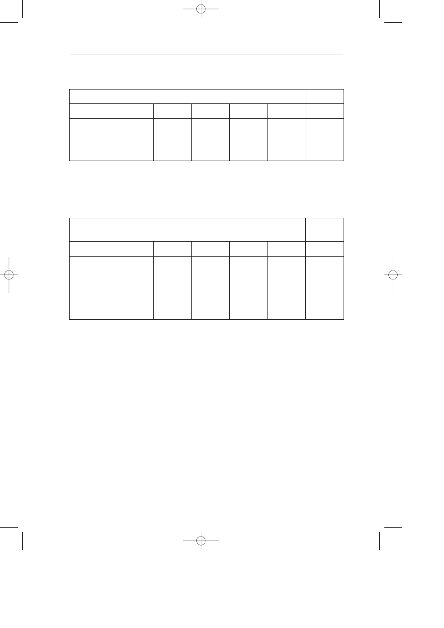
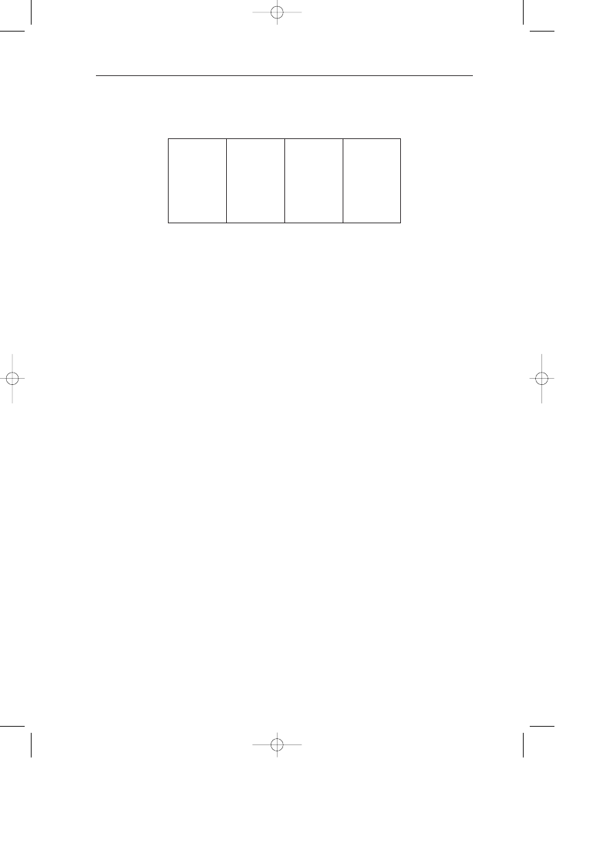
Table 1.1. Results obtained when the plant is fully balanced.
Branches and risers balanced – Thermostatic valves balanced
Total flow
Radiators
1
2
3
4
l/h
Kv thermostatic valve
0.04
0.15
0.25
0.14
Flow (l/h)
11
43
65
33
152
Heat output (W)
255
1000
1512
765
Room t° in °C
20
20
20
20
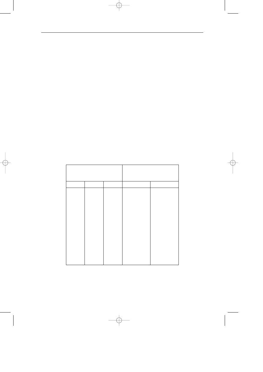
Table 1.2. Risers and branches are balanced, but not the thermostatic valves.
Branches and risers balanced
Total flow
Thermostatic valves not balanced and fully open
Radiators
1
2
3
4
l/h
Kv thermostatic valve
0.8
0.8
0.8
0.8
Flow (l/h)
66
45
30
11
152
Flow (%)
600
105
46
33
Heat output (W)
290
1006
1270
573
Heat output (%)
114
101
84
75
Room t° in °C
24.1
20.2
15.2
12.4
TA-Handbok 3 (GB) 03-04-24 14.25 Sida 8
1 . B A L A N C I N G O F R A D I A T O R S Y S T E M S
9
1.2 Overflows in distribution
An overflow in the distribution creates one or several undesired mixing points
and the actual supply water temperature is lower than expected.
An overflow in the distribution, particularly during the morning start-up, creates an
incompatibility problem between production and distribution. Let us consider two typical
examples.
In Fig 1.2, if the distribution flow q
d
is greater than the production flow qg, the difference
circulates in the bypass in the direction BM. A mixing point is therefore created at M
causing a drop in the supply water temperature. The maximum supply water temperature in
the distribution is lower than the maximum temperature obtained in the boilers. The plant
therefore has difficulties at start-up as the installed power cannot be transmitted. In some
plants, the problem is solved by installing additional boilers, which can increase the pro-
duction flow q
g
, making it compatible with the distribution flow q
d
. This type of solution
is very expensive both in capital cost and in operation as the seasonal efficiency drops.
Fig 1.2. Several circuits are connected to the heating plant through a decoupling bypass.
A
qs
B
M
qs
tr
qg
tgs
tgr
tr
qb
qd
ts
tr
qc
TA-Handbok 3 (GB) 03-04-24 14.25 Sida 9
B A L A N C I N G O F R A D I A T O R S Y S T E M S
10
In Fig 1.3, circuit overflows cause circulation in pipe FE from E towards F with a mixing
point created in D. The last circuit is then supplied from its own return. This circuit
works under particularly bad conditions and becomes the plant’s “nightmare” circuit.
Placing a non-return valve in pipe EF would appear to solve the problem, but it
actually creates another problem as the loop is open and boiler pumps go into series with
circuit pumps, making some control loops unstable.
In conclusion, the most efficient and easiest solution is to correctly balance pro-
duction and distribution ensuring their flow compatibility.
Fig 1.3. Distribution through a closed loop.
qs
qs
tr
qg
tgs
tgr
tr
qp
ts
tr
qc
E
F
D
TA-Handbok 3 (GB) 03-04-24 14.25 Sida 10
2 . R A D I A T O R V A L V E S
11
2. Radiator valves
2.1 General
Radiator valves have several functions. One of them is to isolate the radiator on the inlet
and the outlet. An important function is also to adjust the flow to the required value.
This function can be achieved either by the valve on the inlet or by the return valve.
2.1.1 WHEN THE INLET VALVE IS USED ONLY TO ISOLATE
When the manual valve on the inlet is only used for shut-off function, its oversizing is not
so important. The limitation of the flow at design value is obtained with the valve on the
return, which takes the majority of the differential pressure available. This return valve
must have a profiled cone to get adequate authority on the flow in the range of adjustment.
The presetting of the return valve is made according to the expected available differential
pressure and the required design flow.
The water flow depends on the differential pressure across the valve and its Kv according
to the equation:
The Kv value depends on the degree of opening of the valve. When the valve is fully
open the specific Kv obtained is called the Kvs.
The correct valve can be determined with the help of a nomogram, (see e.g., Fig 4.2).
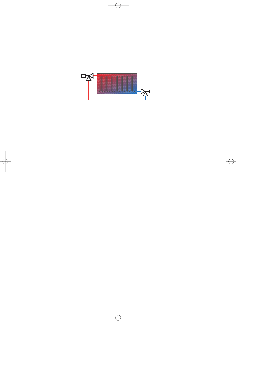
2.1.2 WHEN THE INLET VALVE IS USED TO ISOLATE AND ADJUST
THE FLOW
This manual valve must be provided with a profiled plug to obtain a progressive restriction
of the flow when shutting the valve. This progressiveness only works if the valve is not
oversized and thus has a sufficient authority.
The Kvs of the valve in the inlet is chosen to obtain approximately the design flow for
the valve 75% open. When the available Kvs is too high, one solution is to limit the degree
of opening of this valve to the correct Kv. Another possibility is to install in the inlet a
double regulating valve where the shut-off and regulating functions are independent.
Fig 2.1. Radiator valves on the inlet and the outlet.
q = 100 Kv
√ ∆
p (q in l/h and
∆
p in kPa)
TA-Handbok 3 (GB) 03-04-24 14.25 Sida 11
B A L A N C I N G O F R A D I A T O R S Y S T E M S
12
2.2 What is a thermostatic valve?
A thermostatic valve is a self-acting automatic valve controlled by an expanding element.
Depending on the difference between the temperature set point and the room temperature,
the valve gradually opens or closes.
All the thermostatic valves on the market have a total lift of several millimetres.
However, starting from the valve in shut position, a decrease in the room temperature
of 2K will open the valve about 0.5 mm. This part of the lift, where the control valve
normally works, is called the nominal lift.
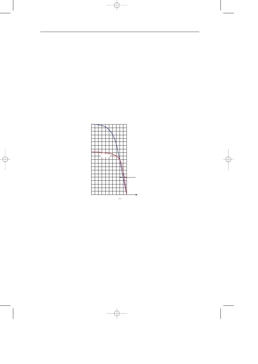
Fig 2.2 shows two relations between the water flow and the room temperature.
Curve a is for an unlimited flow thermostatic valve. Curve b is for a thermostatic valve
with flow limitation. This limitation is obtained with an adjustable resistance in series
with the active port of the valve.
In practice, the thermostatic valve reacts gradually to the changes in the room temperature,
unless the temperature starts to develop in the other direction. In this case the plug of the
valve does not move until the room temperature varies by a value that exceeds the hysteresis
(normally around 0.5K). This phenomenon sometimes gives the impression of a stable heat
transfer from the radiator whereas the control loop can become unstable in the longer term.
Thermostatic valves allow the achievement of the correct temperature in each
room individually. They compensate a possible oversizing of the radiator and reduce
heat output when other sources of heating (lamps, people, sun, etc.) compensate for
part of the heat losses. In this respect, thermostatic valves provide the user with more
flexibility, improve the comfort and save energy.
Fig 2.2. Relation between the water flow and the room temperature for a thermostatic valve supplied
at constant differential pressure. a - unlimited flow valve. b - valve with flow limitation.
a
b - TA
Room temperature
200
100
150
50
0
14
16
18
20
22
Set point
Nominal lift
of 0.5 mm
TA-Handbok 3 (GB) 03-04-24 14.25 Sida 12
2 . R A D I A T O R V A L V E S
13
2.3 Thermostatic valves and the supply water temperature
Controlling the heat output from a radiator with a thermostatic valve is
quite difficult when the supply water temperature is maintained constant during
the whole heating season. For this reason, the supply water temperature is
normally variable and depends, for instance, on outdoor conditions.
As an example, we can take a radiator permanently supplied at 80 °C throughout the entire
heating season. The thermostatic valve is assumed to be correctly sized to give design
flow at nominal opening (80/60 conditions). The minimum outdoor design temperature
is –10 °C.
Fig 2.3 shows the necessary water flow in the radiator as a function of outdoor conditions,
in order to obtain room temperatures of 18, 20 and 22 °C.
Around the mean winter temperature (t
e
= 5 °C), a water flow variation of 4% will
change the room temperature by 2K. To obtain a precise room temperature within ± 0.5K,
the water flow must be controlled with an accuracy of ± 1%. As 50% of the load corres-
ponds to 20% of the flow, the lift of the valve has to be set at an opening of 0.1 mm (20%
of the nominal lift of 0.5 mm), with a precision of ± 0.005 mm (1% of nominal lift)!
Obviously this is impossible, and the thermostatic valve cannot find a stable degree of
opening. It then works in on-off mode with oscillations in the room temperature. When
the thermostatic valve is open, the heat output is much higher than necessary, creating a
transitory increase of room temperature before the thermostatic valve reacts.
Fig 2.3. The necessary water flow to maintain the room temperature constant as a function of
outdoor conditions. The supply water temperature is assumed to be constant and equal to 80 °C.
0
10
20
30
40
50
60
70
80
90
100
10
20
30 40
50
60 70
80
90 100
0
22
°
C
20
°
C
18
°
C
20
°
C
–10
°
C
5
°
C
Outdoor temperature
Water flow in %
Heat losses in %
TA-Handbok 3 (GB) 03-04-24 14.25 Sida 13
B A L A N C I N G O F R A D I A T O R S Y S T E M S
14
This is why the thermostatic valve is normally used with a central controller that modifies
the supply water temperature to suit requirements. These are determined by an outdoor
sensor or by a temperature sensor located in a reference room (not fitted with thermostatic
valves) or by a combination of the two. The thermostatic valve corrects residual variations
as a function of the conditions specific to each room.
In conclusion, the heat output of a radiator cannot be controlled only by varying the
flow. Basic control is obtained by controlling the supply water temperature according to
general needs.
2.4 Is the thermostatic valve a proportional controller?
The thermostatic valve theoretically behaves like a proportional controller. In practice,
working conditions are not always favourable and the thermostatic valve often works as
a temperature limiter. In this case a small proportional band gives better results. Even
then, it may sometimes give the impression of behaving proportionally as it moves into
intermediate, temporarily stable positions, as a function of its hysteresis.
A proportional controller gradually opens or closes the control valve in proportion to
the deviation between the controlled value and its set point.
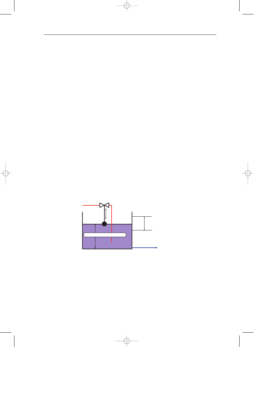
Fig 2.4 shows a level controller. The operation obtained is similar to that of a thermo-
static valve if it is assumed that the water level represents the room temperature. The
flow Z corresponds to the heat losses, and the supply flow Y corresponds to the radiator’s
heat output.
When the level decreases, the float B goes down and opens valve V proportionally to the
level reduction. A balance is obtained when the supply water flow Y equals the flow Z.
When Z = 0, the level rises to H
o
at which valve V is closed. When Z reaches its
maximum value, a stable situation is obtained when valve V is fully open. The float is
then in the H
m
position. The level therefore takes on stable values between H
o
and H
m
depending on the amplitude of disturbances.
Fig 2.4. Analogue representation of a thermostatic valve.
Y = radiator heat output
PB proportional band
Z = heat losses
Y
B
V
H
o
Hm
Z
H = room temperature
TA-Handbok 3 (GB) 03-04-24 14.25 Sida 14
2 . R A D I A T O R V A L V E S
15
This difference H
o
–H
m
is called the proportional band. It is the level variation necessary
to change the control valve from maximum opening to closing.
If this proportional band is reduced to increase the control accuracy, there is a risk
of reaching a critical value at which the control loop becomes unstable. A small propor-
tional band results in a large variation of the flow Y for a small change in the level. This
flow variation may then be larger than the disturbance that caused the change in level,
thus creating a reverse disturbance larger than the initial disturbance. The level then
oscillates continuously.
Reconsider Fig 2.2. The valve is fully closed for a room temperature of 22 °C, and
fully open for t
i
= 14 °C. The proportional band is therefore 8K. However, for a thermo-
static valve with presetting, the design flow is obtained in practice for a room temperature
variation of 2K and it is normal practice to arbitrarily assume that the proportional band of
the thermostatic valve is 2K. We would like to clarify that this 2K is not really the propor-
tional band of a thermostatic valve. The proportional band has to represent the range of
room temperature modifications where linearity is obtained between the room temperature
and the water flow. This control is expressed in terms of % of flow per K of the room
temperature deviation. Therefore, we have adopted, for thermostatic valves, a specific
definition for the proportional band: it’s the double of the deviation in room temperature
which changes the water flow from 0 to 50% of the design value (100% being obtained
for a deviation of 2K). This definition concerns the assembly consisting of thermostatic
valve + radiator + return valve (if there is one).
If we consider now that a return valve or an internal restriction in the thermostatic
valve is used to obtain the correct flow at nominal lift, the resulting curves for some settings
are shown in Fig 2.5.
The set point is chosen so that the flow is less than 100% when the room tempera-
ture exceeds 20 °C.
Fig 2.5. A regulating valve or an internal restriction in the thermostatic valve modifies
the resulting Kv = f (ti) curve and the practical proportional band.
0
0.1
0.2
0.3
0.4
0.5
0.6
0.7
0.8
18
19
20
21
22
1.60 K
0.50 K
1.30 K
Proportional
band
Total Kv
Room temperature
°
C
Set points
TA-Handbok 3 (GB) 03-04-24 14.25 Sida 15
B A L A N C I N G O F R A D I A T O R S Y S T E M S
16
Table 2.1 shows the variation of the proportional band, for three setting examples, when a
restriction reduces the maximum flow.
The real curve between Kv and room temperature also depends on the hysteresis of the
valve as well as the variation of the microclimate around the thermostatic head.
In any case, a proportional band of less than 1K will almost certainly make the valve
work in on-off mode. This is not a serious problem if oscillations of the room temperature
are practically not perceivable, which is the case in balanced plants where the water
temperature is controlled as a function of outdoor conditions. In well-insulated buildings
a narrow proportional band gives more accurate control of room temperature despite the
on-off behaviour of the control loop, which also contributes to reduced energy consump-
tion. When working with wide proportional bands, we may get a stable control. However,
as the temperature is slowly moving within a large span, we don’t save as much energy as
possible. Effectively, we don’t take all the benefit of internal heat or sun energy.
The question is the following: when a thermostatic valve works to compensate for an
internal emission, is it better to have a small or a large proportional band?
Let us consider two different thermostatic valves, set at 20 °C, with the same Kv
but with a proportional band of 2 and 1K respectively.
With a proportional band of 2K, the room temperature can increase to 22 °C before
the radiator emission will be stopped. If the proportional band is only 1K the radiator
will be already isolated for a room temperature of 21 °C. It is then possible to save more
energy when working with small proportional bands.
Kv2
0.65
0.50
0.20
Kv
max
0.80
0.56
0.20
BP
1.60
1.30
0.50
SP
20.00
19.7
18.90
ST
22.00
21.7
20.90
Kv2
= (Kv at
∆
T 2K) Kv at nominal lift corresponding to a deviation of 2K,
this Kv corresponds to the design Kv.
Kv
max
= Kv obtained with the valve fully open.
PB
= Proportional band
SP
= Set point adopted for a required room temperature of 20 °C.
ST
= Room temperature at which the valve is completely shut.
Table 2.1. Variation of the proportional band of one thermostatic valve
under the effect of a restriction in series.
TA-Handbok 3 (GB) 03-04-24 14.25 Sida 16

2 . R A D I A T O R V A L V E S
17
2.5 Should a plant be hydraulically balanced
with all thermostatic valves fully open?
The answer is yes and the thermostatic valves must have a saturated characteristic.
Balancing the radiators in a circuit results in obtaining correct flows in each radiator at
design condition. At intermediate loads, flows and pressure drops in pipes are reduced,
differential pressures increase and each radiator can at least obtain its design flow.
Some consider that all thermostatic valves should be set to their nominal opening
before balancing a plant. This appears logical as flows are normally determined in these
conditions. The thermostatic heads should then be replaced by graduated caps for setting
the valves at their nominal lift.
Whenever the plant is started up, after the night setback, thermostatic valves are
opened beyond their nominal opening and will be in overflow, creating underflows in
other parts of the plant. The purpose of balancing is thus not achieved.
This situation is difficult in the case of an unlimited flow thermostatic valve such
as that shown in Fig 2.2a. Moreover, overflows are permanent on valves for which the
thermostatic head has been removed.
Thermostatic valves with an interchangeable plug, allowing the achievement of the
right Kv, normally don’t have a flat enough curve to solve the problem.
The problem is related to the big difference in flows between the valve fully open
and the valve at nominal lift (Fig 2.2a). Solving this problem is quite simple: the valve
characteristic has to be saturated. It means that the flow will not significantly increase
beyond the nominal opening (Fig 2.2b). This is obtained with a resistance in series with
the thermostatic valve (Fig 2.5). In this case, the flow/opening curve beyond the nominal
lift is so flat that the plant can be balanced with all thermostatic heads removed.
This discussion demonstrates the necessity to balance the plant with all thermostatic
heads removed and to use thermostatic valves with a small difference between the design
and the maximum flows, this means with a saturated characteristic as shown on Fig 2.5.
However, in the case of an occupied building, the operation of removing all thermo-
static heads and replacing them after balancing is a difficult operation. Sending circulars
asking occupants to carry out this operation is not a particularly reliable method. Some
installers prefer to do the balancing during the heating season; they reduce the hot water
temperature significantly the day before, inciting occupants to fully open their thermostatic
valves.
TA-Handbok 3 (GB) 03-04-24 14.25 Sida 17
2.6 Accuracy to be obtained on the flow
In most cases the flow has to be adjusted with an accuracy of ± 10%.
In section 1 we considered the disadvantages of hydronic unbalances in plants. Before
studying balancing procedures, we must define the precision with which flows have to be
adjusted.
In practice, flow adjustment precision depends on the required room temperature
precision. This precision also depends on other factors such as control of the supply water
temperature and the relation between the required and installed capacity. There is no
point in imposing a very high accuracy on the flow if the supply water temperature is
not controlled with an accuracy producing equivalent effects on the room temperature.
An underflow cannot be compensated by the control loop, and has a direct effect on
the room temperature under maximum load conditions; it must therefore be limited. An
overflow has no direct consequence on the room temperature since in theory, the control
loop can compensate for it. However, when the control valve is fully open, for example,
when starting up the plant, this overflow produces underflows in other units and makes
distribution incompatible with production. Overflows must therefore also be limited.
Table 2.2 compares the influence of the flow on the room temperature under well-
defined design conditions.
B A L A N C I N G O F R A D I A T O R S Y S T E M S
18
Design
Allowable deviation in % of
design water flow, for a room
temperature accuracy of 0.5K
t
ec
t
sc
t
rc
– 0.5K
+ 0.5K
0 90 70
–
15
+21
82 71 –
24
+44
– 10
93
82
– 21
+34
90 70 –
12
+15
90
40
– 4
+ 4
80 60 –
10
+13
80
50
– 7
+ 7
80
40
– 4
+ 5
60
40
– 8
+ 9
55
45
– 15
+ 20
– 20
90
70
– 10
+13
80 60
–
9
+10
80
40
– 4
+ 4
75
45
– 5
+ 6
70
45
– 6
+ 7
60
40
– 7
+ 8
55 45 –
13
+17
Table 2.2. Variations of the flow q in the radiator to modify
the room temperature by 0.5K at full load.
TA-Handbok 3 (GB) 03-04-24 14.25 Sida 18

Let us take an example for a heating plant working with the following design conditions:
Supply water temperature t
sc
= 80 °C, return t
rc
= 60 °C and room temperature t
ic
= 20 °C.
The design outdoor temperature is tec = –10 °C. A room temperature variation of 0.5K
can be obtained by reducing the water flow by
∆
q = 10%.
The water flow adjustment accuracy must be better when the plant is working with
a relatively high thermal effectiveness
Φ
.
For a rough conclusion, we can see that water flows have to be controlled with an
accuracy of ± 10 to ± 15%. Concurrently, the water temperature has to be controlled with
an accuracy of ± 1 to ± 1.5K.
We may be tempted to accept overflows, especially when they have little effect on
the room temperature. This would neglect the pernicious effects of overflows which create
underflows elsewhere making it impossible to obtain the required water temperature at high
loads, due to incompatibility between production and distribution flows (see section 1.2).
2 . R A D I A T O R V A L V E S
19
TA-Handbok 3 (GB) 03-04-24 14.25 Sida 19

B A L A N C I N G O F R A D I A T O R S Y S T E M S
20
3. Radiators
3.1 Nominal and design conditions
A radiator heat output is to be defined for a given room temperature (20 °C), water supply
and return temperatures, for example 75 and 65 °C. The temperatures of 20, 65 and 75 °C
are nominal values of the room temperature and water temperatures. They are identified
by the subscript “n” (for example t
in
= nominal room temperature). Nominal values are
actually catalogue values used by manufacturers; they determine the conditions under
which the power of a unit is defined. According to European norms EN442, the nominal
power of a radiator is valid for a supply water temperature of 75 °C, a return water
temperature of 65 °C and a room temperature of 20 °C. But, normally, a radiator does not
work in these conditions. Then, the required design water flow in the radiator must be
determined in each particular case. It is obviously meaningless to try to adjust the water
flow in a radiator if this flow is not correctly determined.
The plant is calculated in certain conditions with specific values for the controlled
variables, outdoor conditions, supply and return water temperatures. Those values, used
to calculate the plant, are the design values; they are identified by a subscript “c” (values
used for calculations).
3.2 Selection of a radiator not working in nominal conditions
Radiator heat output in catalogues refers to nominal conditions, for example, water
supply temperature t
sn
= 75 °C, return temperature t
rn
= 65 °C and a room temperature
t
in
= 20 °C. How is a radiator selected if it does not work in these conditions?
The real transferred power P is related to the nominal power P
n
as follows:
No subscript: present conditions
Subscript n: nominal conditions.
t
s
= Supply water temperature.
t
r
= Return water temperature.
t
i
= Room temperature.
n = This exponent for radiators is normally taken = 1.3
This formula expresses the influence of the temperature geometric average between the
radiator and the room. This formula is translated into a graph on figure A1 in appendix A
where some specific examples are explained.
(
t
s
– t
i
) (
t
r
– t
i
)
inncccfff cccccci
(
t
sn
– t
in
) (
t
rn
– t
in
)
P = P
n
×
(
)
n/2
TA-Handbok 3 (GB) 03-04-24 14.25 Sida 20
3 . R A D I A T O R S
21
Example: What is the nominal power 75/65 of a radiator which has to deliver 1000 W
in a room at 22 °C when the actual supply and return water temperature are respectively
72 and 60 °C respectively?
In Fig A1 (Appendix A), join t
s
– t
i
= 72 – 22 = 50 to t
r
– t
i
= 60 – 22 = 38 to find
Sp = P
n
/P = 1.18. The nominal power to install is 1000 x 1.18 = 1180 W.
This formula is theoretical as it assumes that the water flow is distributed uniformly in
the radiator.
Heat output is also affected by a window sill above the radiator that may reduce
heat output by 35%. A radiator close to a window generates hot air circulation and
supplementary heat losses through the window, reducing the energy really transmitted in
the room. The nominal power of a radiator is determined in favourable conditions, which
are not always reproduced in practice. A coefficient of security remains necessary when
a radiator is selected.
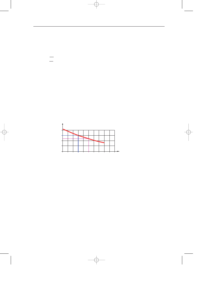
3.3 Emission of a radiator as a function of the water flow
The required water flow in the radiator can be calculated using the following equation:
q: flow in l/h P: heat output in W
∆
T: temperature drop in K
For a 1000 W radiator and a design temperature drop of 20K, the required water flow
is 0.86
×
1000 / 20 = 43 l/h.
However, when the flow varies, the water temperature drop also varies which makes
the relation between the flow and heat output non-linear.
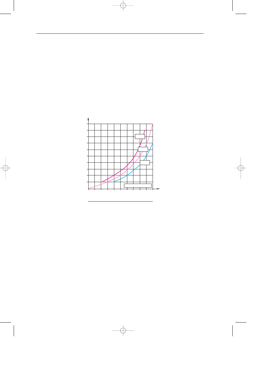
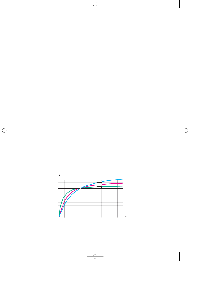
Fig 3.1 shows this relation for a supply water temperature of 80 °C and various
temperature drops
∆
T
c
.
0.86
×
P
cc cci
∆
T
q =
Fig 3.1. Heat output, in a room at 20 °C, as a function of the water flow, for a radiator (n = 1.3)
and for different water
∆
T
c
values. t
sc
= 80 °C.
Φ
= 0.50
Φ
= 0.33
Φ
= 0.17
P %
q %
0
10
20
30
40
50
60
70
80
90
100
11
120
130
50
100
150
200
250
300
80/5
80/6
80/7
TA-Handbok 3 (GB) 03-04-24 14.25 Sida 21

B A L A N C I N G O F R A D I A T O R S Y S T E M S
22
At the origin, the gradient of the “heat emission/flow” curve is the inverse of the thermal
effectiveness “
Φ
” of the radiator. This thermal effectiveness is defined as follows:
∆
T
c
= design water temperature drop.
∆
T
o
= water temperature drop at zero load = t
sc
– t
ic
For 80/60 design conditions, the thermal effectiveness
Φ
is: (80 – 60) / (80 – 20) = 0.33
and the increased power at the origin is 1/0.33 = 3% power per % of flow.
At design condition, an overflow in the radiator does not significantly increase the
emitted heat, particularly when the thermal effectiveness is low.
3.4 Selection of the design water temperature drop
For a supply water temperature between 70 and 90 °C, it’s quite common to design the
plants for a
∆
T = 20. This magic value has been adopted for many years and translated
into local units (20 °C in continental Europe and 20 °F (11 °C) in the UK and USA, for
instance). However, to reduce the return water temperature in district heating or when
using condensing boilers, a higher
∆
T is adopted. The design
∆
T depends mainly on the
habits in each country, but it can be optimised according to each specific plant.
Radiators working with a low water temperature drop
∆
T
c
have a strongly saturated
response curve P% = f (q%). Flow variations therefore have little influence on the max-
imum emission. However, these radiators become difficult to control at low loads since
the emission is very dependent on the flow in this zone.
The use of a high
∆
T
c
can reduce water flows, pumping costs, pipe diameters and
losses. Control of the radiator is also improved. However, the maximum power becomes
more sensitive to the water flow, requiring a precise hydronic balancing of the plant.
A high value of
∆
T
c
reduces heat exchanges, thus requiring the use of radiators with
larger surface areas. For example, the use of a
∆
T
c
of 30K instead of 20K reduces the heat
exchange approximately by 16%.
The optimum
∆
T depends on each plant. Increasing the
∆
T reduces the water flows,
the sizes of the pipes and accessories, the pumping costs and the heat losses in pipes but
radiator surfaces have to be increased. The optimum
∆
T can therefore be calculated for
each plant.
∆
Tc
∆
To
φ
=
TA-Handbok 3 (GB) 03-04-24 14.25 Sida 22
3 . R A D I A T O R S
23
3.5 Existing plants
How to compensate for oversized radiators after an improvement
of the insulation of the building.
Existing plants can be treated in the same way as new plants. However, improvements
may have been made to the building, considerably reducing heat losses. Radiators will
then be oversized with respect to the initial conditions.
If the thermal insulation was improved uniformly, the heat output of the radiators is
adjusted to new conditions by reducing the water supply temperature.
An example of a calculation: Take, for instance, a radiator with a nominal power of
1200 W in conditions 75/65. The design power required is, for instance, 1000 W for a
supply water temperature of t
s
= 80 °C in a room temperature of t
i
= 20 °C. What flow
should the radiator have?
The nominal oversizing factor is S
pn
= P
n
/P = 1200/1000 = 1.2.
Referring to Fig A1 in appendix A, join t
s
– t
i
= 80 – 20 = 60 °C to P
n
/P = 1.2
to find t
r
– t
i
= 31.2 °C. Then t
r
= 51.2 and
∆
T = 80 – 51.2 = 28.8 K. Finally, q =
0.86
×
1000/ 28.8 = 30 l/h.
Fig A2 can also be used. Join t
s
– t
i
= 80 – 20 = 60 °C to P
n
/P = 1.2 to find q =
30 l/h per 1000 W.
In most plants, thermal insulation is not improved uniformly and each radiator has to be
treated independently as in section 3.2.
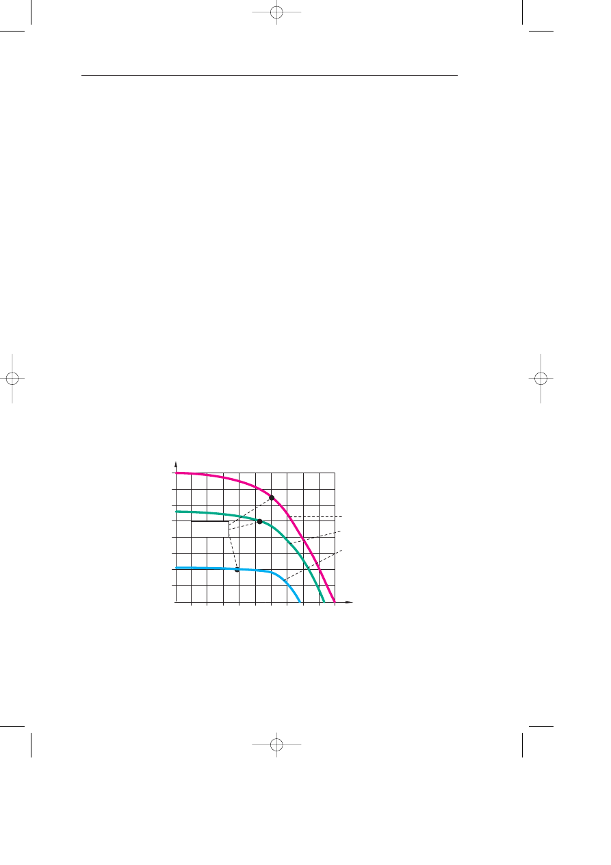
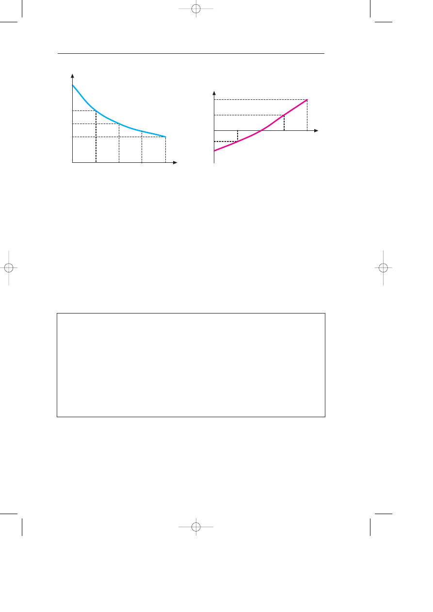
Fig 3.2. When the designed
∆
T is increased, the water flow decreases but
the required radiator surfaces increase (t
s
= 80 °C ).
10
200
133
100
66
30
25
20
15
Flow %
∆
T
P
n
/ P
c
= Relative radiator oversizing
∆
T
0.87
0.93
1.00
1.10
1.20
10
30
25
20
15
t
s
= 80
°
C
t
s
= 80
°
C
TA-Handbok 3 (GB) 03-04-24 14.25 Sida 23
B A L A N C I N G O F R A D I A T O R S Y S T E M S
24
4. Two-pipe distribution
4.1 Balancing of radiators based on a constant
∆
p
To set the Kv of the thermostatic valves, the differential pressure
is considered to be of
∆
H
o
= 10 kPa, for instance. This differential pressure
is automatically obtained after balancing the distribution.
4.1.1 CHOOSING THE DESIGN DIFFERENTIAL PRESSURE
If a flow measurement device is available at each radiator, a standard balancing procedure
can be used and a balancing valve on the circuit acts as a partner valve. This can keep
previously adjusted radiator flows constant while others are being adjusted (the com-
pensated method). However, thermostatic valves are generally preset according to
calculated values.
The main pressure drop is in the thermostatic valve with adjustable Kv as the pressure
drop in the radiator is normally low. Since some inaccuracy is acceptable on flows, we
can assume that each radiator in a branch is subject to the same differential pressure
∆
H
o
.
This differential pressure must not be too high to maintain an adequate cross-section at
the valve, thus reducing risks of clogging and noises. This differential pressure must not
be too low either, in which case the relative influence of pressure drops in circuit pipes
cannot be neglected. Therefore, the differential pressure
∆
H
o
is generally chosen between
8 and 10 kPa.
Fig 4.1. Each radiator valve is adjusted as if it were subject to the same differential pressure
∆
H
o
.
STAD
∆
H
o
TA-Handbok 3 (GB) 03-04-24 14.25 Sida 24
4 . T W O - P I P E D I S T R I B U T I O N
25
Each adjustable thermostatic valve is then preset based on this selected differential pressure
∆
H
o
. When the balancing valve STAD on the branch is adjusted to obtain a total flow
corresponding to the sum of the flows in the radiators, the preliminary settings made are
justified. The selected differential pressure
∆
H
o
is then applied across the hydraulic centre
of the circuit. In practice, the first radiator will be in slight overflow and the last radiator
will be in slight underflow. These differences depend on the circuit length and on the
pressure drops in the pipes and accessories.
Example: A circuit with radiators, each having a design flow of 50 l/h. The pressure
drop in the pipes is 2 kPa. Consider
∆
H
o
= 8 kPa.
Flow in the first radiator is = 50
×
√
= 53 l/h, and in the last =
50
×
√
= 47 l/h
The deviation is ± 6%.
Consider now
∆
H
o
= 2 kPa and the same pressure drop in the pipes.
Flow in the first radiator is = 50
×
√
= 61 l/h, and in the last =
50
×
√
= 35 l/h
The deviation is –30 to +20%.
This example confirms that
∆
H
o
should be at least 8 kPa.
8 + 1
11
8
11
8 – 1
11
8
11
2 + 1
11
2
11
2 – 1
11
2
11
TA-Handbok 3 (GB) 03-04-24 14.25 Sida 25
B A L A N C I N G O F R A D I A T O R S Y S T E M S
26
4.1.2 PRESETTING THE THERMOSTATIC VALVE
Table 4.1 gives the Kv values to be taken according to the
∆
H
o
adopted.
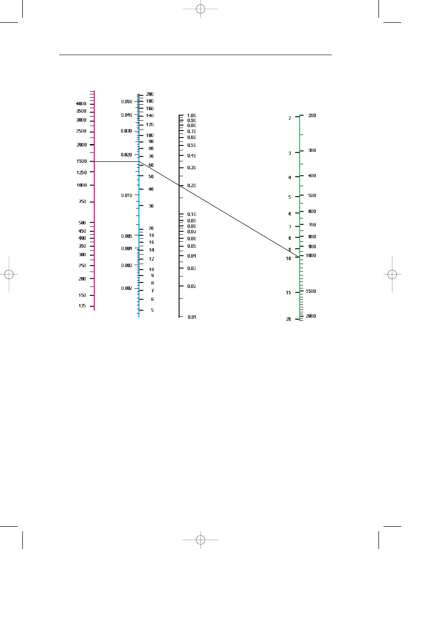
Example: For a 1500 W radiator working with a
∆
T of 20K and a differential pressure
of 10 kPa, the Kv value of the thermostatic valve must be 0.2. Use the chart in Fig 4.2
to find the Kv value graphically.
Table 4.1. Determining the Kv of a thermostatic valve.
Working conditions
Kv valve for
∆
Ho =
10 kPa
Heat output in (W)
Water flow
∆
T = 10
∆
T = 20
l/h
l/s
Kv
250
500
21.5
0.006
0.068
300
600
25.8
0.007
0.082
350
700
30.1
0.008
0.095
400
800
34.4
0.010
0.109
450
900
38.7
0.011
0.122
500
1000
43.0
0.012
0.136
600
1200
51.6
0.014
0.163
700
1400
60.2
0.017
0.190
750
1500
64.5
0.018
0.204
800
1600
68.8
0.019
0.218
900
1800
77.4
0.022
0.245
1000
2000
86.0
0.024
0.272
1100
2200
94.6
0.026
0.299
1200
2400
103.2
0.029
0.326
1250
2500
107.5
0.030
0.340
1300
2600
111.8
0.031
0.354
1400
2800
120.4
0.033
0.381
1500
3000
129.0
0.036
0.408
1750
3500
150.5
0.042
0.476
2000
4000
172.0
0.048
0.544
2250
4500
193.5
0.054
0.612
TA-Handbok 3 (GB) 03-04-24 14.25 Sida 26
4 . T W O - P I P E D I S T R I B U T I O N
27
Fig 4.2. Determining the Kv of a thermostatic valve.
For a radiator of 1500 W, the water flow = 64.5 l/h. For a
∆
p of 10 kPa, Kv = 0.2
q
P
Kv
mm WG
kPa
Kv
l/h
l/s
Watt
(
∆
T = 20K)
Kv
∆p
TA-Handbok 3 (GB) 03-04-24 14.25 Sida 27
B A L A N C I N G O F R A D I A T O R S Y S T E M S
28
4.1.3 NON-PRESETTABLE THERMOSTATIC VALVES
When a thermostatic valve is non-presettable, the adjustment will be made on the return
valve. As the thermostatic valve already creates some pressure drop at nominal opening,
only the rest of the available
∆
p is applied across the return valve.
Example: A 2000 W radiator working with a
∆
T = 20K is supplied at a differential
pressure of 10 kPa. The thermostatic valve has a Kv = 0.5. What Kv should be set
at the return valve?
Referring to Fig 4.2, it can be seen that the radiator flow is 86 l/h. At this flow,
the pressure drop in a valve with Kv = 0.5 is 2.96 kPa. The rest is for the return
valve: 10 – 3 = 7. Using the same diagram, we find that the Kv must be 0.33 for a
flow of 86 l/h and a pressure drop of 7 kPa. If we had neglected the pressure drop in
the thermostatic valve, we would have found a Kv of 0.27 for the regulating valve.
The flow obtained would have been 75 l/h instead of the predicted 86, representing
a deviation of 13%.
The same procedure may be used if pressure drops in other resistances, such as elbows,
high resistance radiators, etc., have to be deducted.
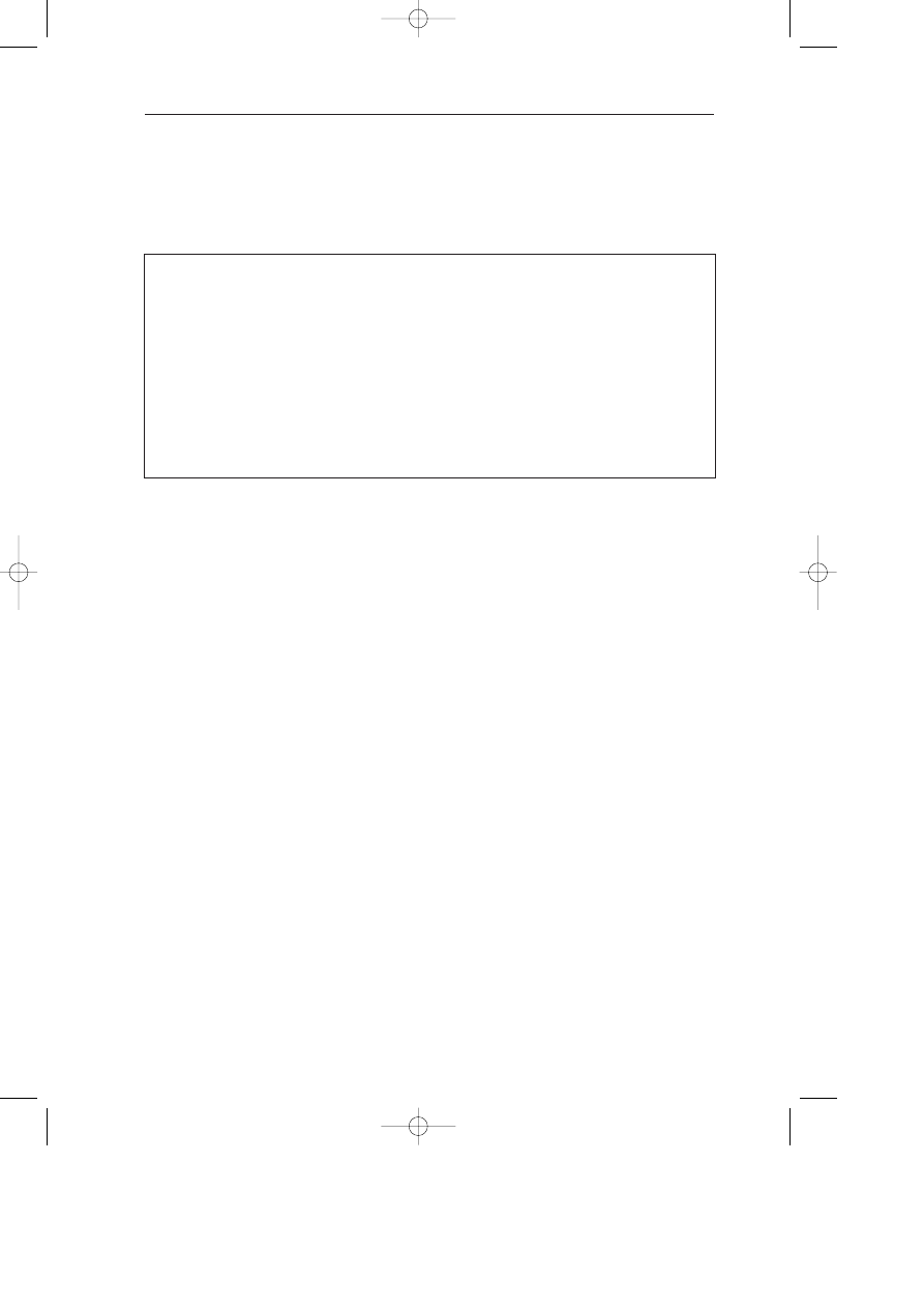
4.1.4 LIMITATIONS OF CHOICE WITH THE SAME
∆
P FOR ALL RADIATORS
The assumption that the same differential pressure is applied to all radiators has some
limits, depending mainly on the required flow accuracy.
Consider the case in Fig 4.3. Valves are preset based on an average differential
pressure
∆
H
o
. The flow will be higher than the design flow at the start of the circuit, and
lower at the end. For a deviation of
∆
q in % of design flow, the maximum allowable length
for pipes is determined in Fig 4.3.
TA-Handbok 3 (GB) 03-04-24 14.25 Sida 28
4 . T W O - P I P E D I S T R I B U T I O N
29
Consider the case of a plant designed for conditions t
sc
= 80 °C and t
rc
= 60 °C. A
deviation in the room temperature in the order of 1K due to the flow is accepted, which
implies a flow precision of
∆
q = ± 20%.
∆
H
o
= 10 kPa is adopted, and the pressure drop in
the circuit considered equals 100 Pa/m (
∆
H
o
/R = 0.1). The method described may there-
fore be used if the distance measured on the pipe between the circuit inlet and last radia-
tor does not exceed 44 metres (See Fig 4.3).
4.2 Presetting based on calculated
∆
p
If pressure drops in pipes are high, the maximum circuit length is quickly restricted.
In this case the differential pressure applied to each radiator must be estimated using the
following formula:
∆
H: Differential pressure in kPa available for a thermostatic valve,
R: Pressure drop in pipe in Pa/m,
L: Distance in metres of pipe between the balancing valve of the branch and a radiator.
This
∆
H is then calculated, for each radiator, to determine the corresponding Kv.
Fig 4.3. When all valves are calculated based on the same
∆
p =
∆
H
o
, the circuit length
should not exceed a given value (
∆
H
o
in kPa and R (pressure drop in pipes) in Pa/m).
0
10
20
30
40
50
60
70
80
0
5
10
15
20
25
?q max %
L
max
in m
∆
H
o
/R
0.15
0.10
0.08
0.06
0.04
0.02
∆
q
max
in %
∆
H
max
∆
H
o
L
max
STAD
∆
H
min
∆
H =
∆
H
max
– =
∆
H
0
+
2RL
cc cci
1000
RL
max
– 2RL
cc c ci
1000
TA-Handbok 3 (GB) 03-04-24 14.25 Sida 29

B A L A N C I N G O F R A D I A T O R S Y S T E M S
30
4.3 Constant or variable primary flow
Primary distribution can be designed for constant or variable flow.
This affects the solutions that can be used to obtain the correct differential
pressure on the secondary distribution.
Local distribution through thermostatic valves is necessarily a variable flow distribution.
However, the primary general distribution may be designed for a constant or a variable
water flow.
The advantage of a constant primary flow in the main distribution is that it keeps the
pressure drops in the pipes constant. The differential pressure on each circuit is adjusted at
the correct value at design condition and does not change with the load. However, the
return water temperature is not minimised, which can be a disadvantage in some district
heating plants and when condensing boilers are installed.
The advantage of a variable flow in the main distribution is that it minimises the
pumping costs and reduces the return water temperature when required. However, at small
loads, the differential pressure on the circuits increases according to the reduction of the
pressure drops in the pipes and accessories when the flow is reduced.
In all cases, the plant has to be balanced to avoid overflows that create underflows
in unfavoured sections and incompatibility problems. For a variable flow distribution,
balancing is made for design conditions, which guarantees that all circuits will obtain at
least their design flow in all working conditions.
4.3.1 ABOUT NOISE
A hydraulic resistance in a circuit creates a pressure drop and a part of the energy is trans-
formed into heat and another part into noise. The risk of noise increases with the differ-
ential pressure.
Some norms define the maximum noise level acceptable in a bedroom to be 30 dBA
during the night and 35 dBA during the day.
In a presettable thermostatic valve, the differential pressure is taken in the presetter,
which limits the flow at design value, and the control port which adjusts the flow to
obtain the required room temperature.
During night setback, the supply water temperature is reduced and the control port
is fully open. The noise created by the valve in these conditions comes from the presetter.
The geometry of the valve and particularly the design of the presetter are important
in order to obtain a “silent” valve.
All tests realised show that noise increases with the water flow. This is another reason
to carefully balance the radiators, avoiding overflows.
TA-Handbok 3 (GB) 03-04-24 14.25 Sida 30

4 . T W O - P I P E D I S T R I B U T I O N
31
The risk of noise could be reduced dramatically during night-time by decreasing the
pump head, simultaneously reducing the differential pressure and the water flow. This
can be obtained, for instance, with a variable speed pump with different settings during
night and day.
During the day, when the thermostatic valve has to compensate for internal heat, the
control port partly shuts. The differential pressure applied on the control port increases
whilst the water flow decreases. The risk of noise is at maximum when the valve is close
to closure. Vibrations occur when the valve is connected the wrong way with the flow of
water going in the reverse direction.
Noise in a plant can have many causes. A radiator or convector can amplify noise
generated by the pump.
Noise can also increase dramatically when the plant is not well vented. Low water
temperatures make it more difficult to vent. Increasing the water temperature during
venting procedure can be a solution whenever possible.
A too low static pressure in some parts of the plant should also be avoided as the air
separates out of the water in a restriction because of the lower local pressure resulting
from the high water velocity.
When a thermostatic valve shuts, the pressure drop in the pipes and restrictions de-
crease. The differential pressure on the thermostatic valve increases which increases the
risk of noise. For this reason, it is not a good idea, in big plants, to adjust the flow with just
one restriction in series with the thermostatic valve. If this thermostatic valve shuts, the
entire pressure drop taken previously in the restriction is transmitted to the control port. It
is much better to take parts of the excess differential pressure in balancing valves in the
branches and risers and the rest, 10 kPa for example, in the presetter associated with the
thermostatic valves. When one thermostatic valve shuts, the water flow and then the
pressure drop in the balancing valves in branches and risers do not change much.
Consequently, the differential pressure on the thermostatic valve increases just a little.
However, if all the thermostatic valves shut simultaneously, all pressure drops in pipes
and restrictions disappear and the thermostatic valves are submitted to the full pump
head. If this happens, the control of the supply water temperature has to be reconsidered.
For instance, the supply water temperature can be reduced when the total water flow in
the plant decreases.
The situation can be more difficult if the pump is oversized and works with a steep
curve increasing the pressure at small loads. For this reason, an adjustable and controlled
pump head is generally more convenient. The pump head can also be reduced during
most of the time and just put at its maximum value during cold seasons. The reduction of
the pump head in warmer seasons is compensated by a small increase of the water supply
temperature.
When, in extreme circumstances, the differential pressure exceeds the limit defined
by the thermostatic valve manufacturer, the differential pressure has to be limited locally.
This question will be examined in the next sections.
TA-Handbok 3 (GB) 03-04-24 14.25 Sida 31
B A L A N C I N G O F R A D I A T O R S Y S T E M S
32
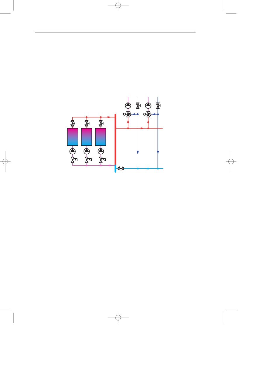
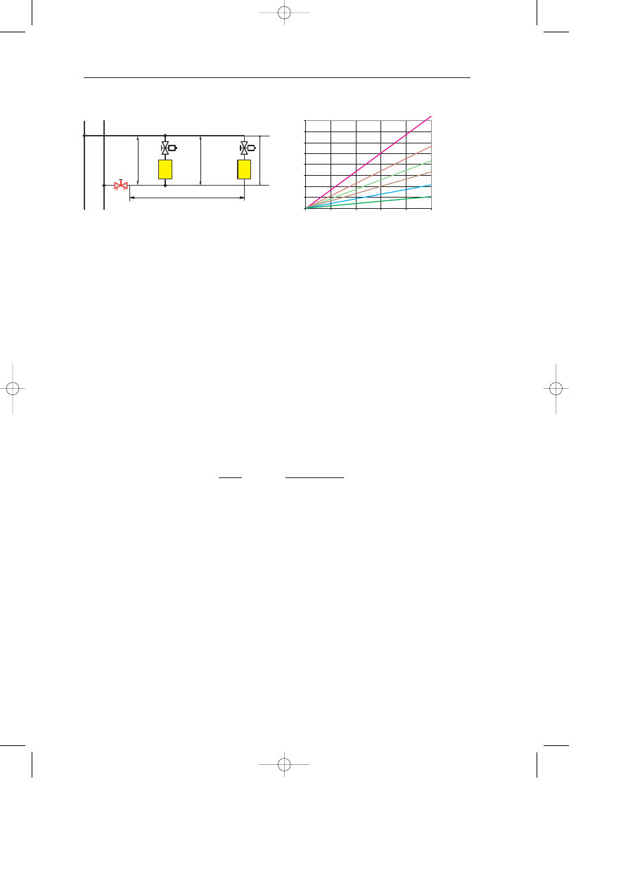
4.3.2 CONSTANT PRIMARY FLOW
Fig 4.4 shows two different circuits applicable to an apartment.
In principle, the water temperature of the distribution is modified to suit outdoor
conditions. A correct distribution of primary flows is obtained by adjustment of balancing
valves STAD.
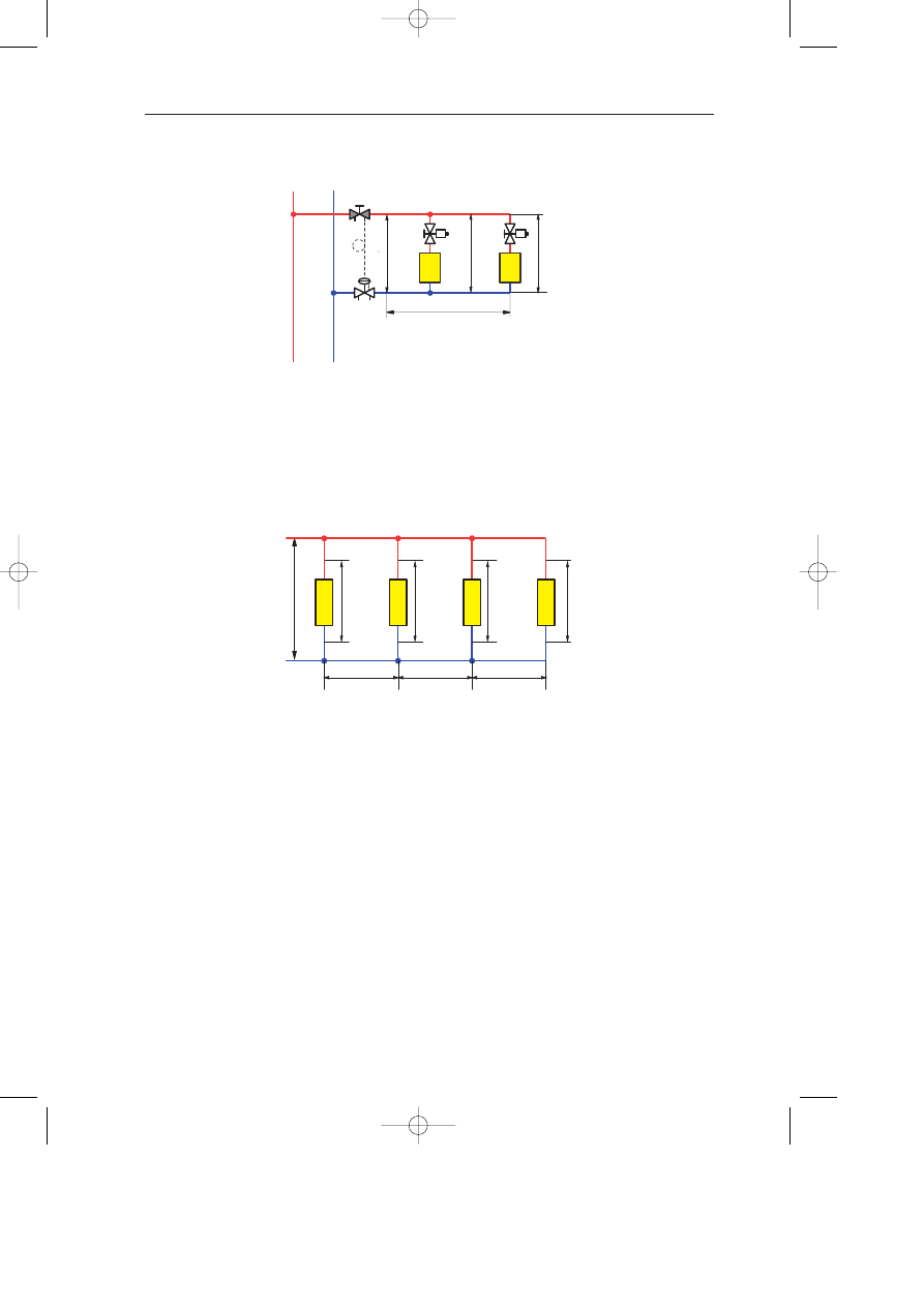
4.3.2.1 A bypass and a secondary pump minimise the
∆
p on the branch
(Fig 4.4 - circuit a).
This circuit is widely used in some European countries. A bypass pipe AB makes the
secondary circuit hydraulically independent of the primary distribution. The high differ-
ential pressure in the main distribution network is not transmitted to the circuit. This
circuit is provided with a circulating pump which can be controlled by a thermostat located
in a reference room. Thermostatic valves are only subject to the relatively low-pressure
head of the secondary circulating pump, decreasing the risk of noise considerably.
Fig 4.4. Two circuits with radiators are designed to give a constant primary flow.
=
A
B
BPV
STAD
STAD
a
b
TA-Handbok 3 (GB) 03-04-24 14.25 Sida 32

4 . T W O - P I P E D I S T R I B U T I O N
33
It is essential that the maximum secondary flow is less than the constant primary flow.
Otherwise, at full load, the difference between the two flows will circulate from B to A,
creating a mixing point at A. In this case, the supply water temperature will be lower than
the design value and comfort is not guaranteed.
A BPV (proportional relief valve) may be installed at the end of the circuit and set
at 10 kPa for example.
The principle application of this BPV is to be closed except when the flow through
the thermostatic valves drops below a certain value, thereby securing the following:
– A limitation of the maximum
∆
p on the thermostatic valves.
– A minimum flow for protection of the circuit pump.
– A prevention of large water temperature drops in the pipes. This is the main reason,
in this case, to install the BPV at the end of the circuit instead of in the beginning.
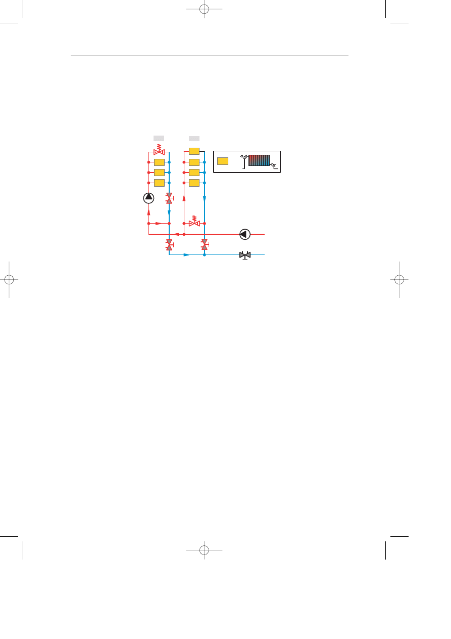
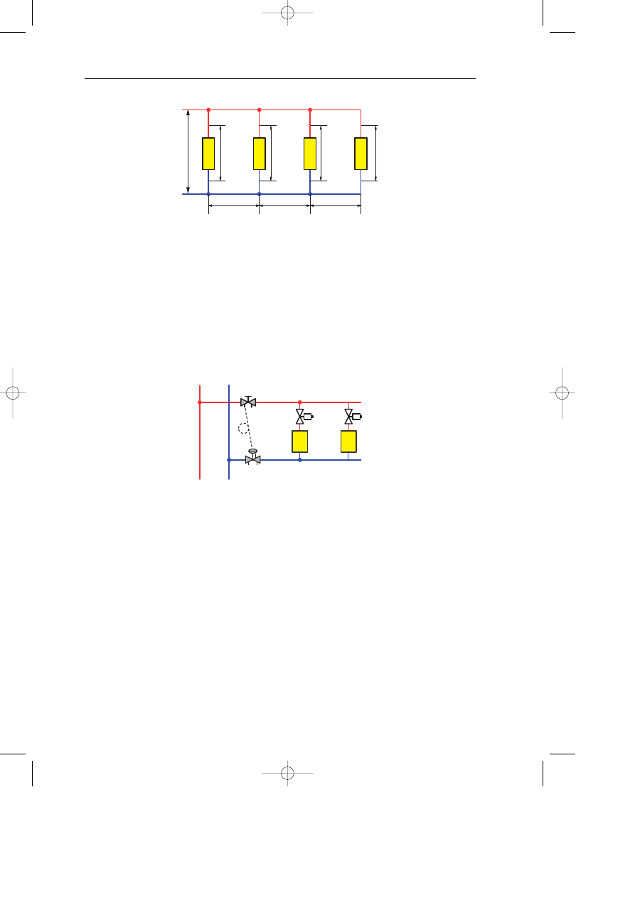
4.3.2.2 A BPV stabilises the
∆
p on the branch (Fig 4.4 circuit b).
A proportional relief valve BPV is placed at the circuit inlet. It gradually opens when the
differential pressure across it reaches its set point. Radiator valves have been set based on
a given differential pressure, for example 10 kPa.
The BPV is kept shut throughout the balancing procedure.
When balancing is complete, with thermostatic valves open, the BPV set value is
reduced until it starts to open. This causes an increase of flow, which can be measured at
STAD. The BPV set point is then increased until it closes again. In some plants, the BPVs
are set to obtain a small flow at design condition; this greatly reduces the circulation noises
in the plant. The explanation for this is related to the pressure waves generated by the
pump, which are bypassed by the BPV.
During normal operation, whenever some thermostatic valves close, the pressure
drop across STAD is reduced and the differential pressure applied to the BPV increased.
The BPV then opens to maintain this differential pressure at its set value. The total primary
flow remains practically constant for a constant
∆
H.
Note that this function is obtained by the combination of the BPV and STAD. Both
elements are essential to keep the total flow and the differential pressure across the circuit
constant. The BPV allows a certain supplementary flow through STAD that creates a
supplementary pressure drop to compensate an eventual increase of the primary differential
pressure
∆
H. Without the STAD, the BPV is not operative.
This distribution method is more efficient than the method that uses a secondary
pump as shown in the circuit a. The secondary pump is eliminated. The protection against
low flows is no longer necessary and the secondary balancing valve is eliminated. Finally,
this pump head is chosen according to need and is maintained constant.
TA-Handbok 3 (GB) 03-04-24 14.25 Sida 33
B A L A N C I N G O F R A D I A T O R S Y S T E M S
34
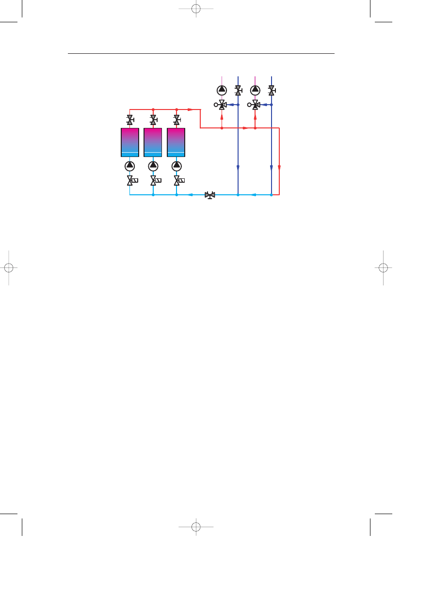
4.3.3 VARIABLE PRIMARY FLOW
In order to minimise return water temperatures, a variable flow distribution has to be
adopted. This is often essential when the plant is connected to a district heating distribution.
Two examples are shown in Fig 4.5.
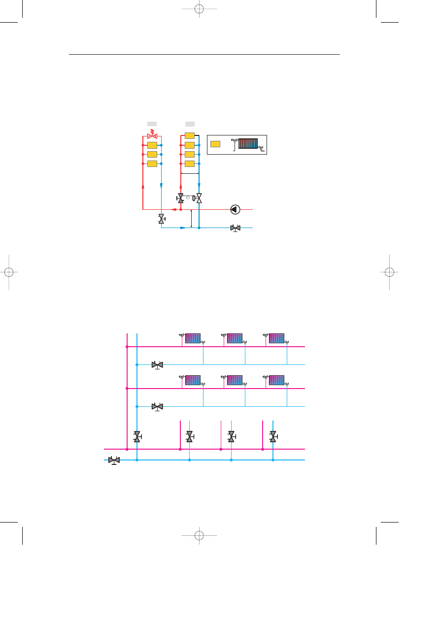
4.3.3.1 A plant with balancing valves (Fig 4.5 – circuit a).
This is the classic case of a branch or a small riser connected to a main network. Thermo-
static valves are preset for a given differential pressure, for example, 10 kPa. The
balancing valve STAD is used to obtain the total flow in circuit “a”, which at design
condition gives the selected differential pressure of 10 kPa at the hydraulic centre of
gravity of the circuit, and more than 10 kPa at other loads.
Fig 4.5. Two circuits supplied at variable primary flow.
=
STAD-0
STAD
a
b
∆
H
∆
p
STAP
STAM
STAD
STAD
Fig 4.6 The installation is balanced using the TA method.
TA-Handbok 3 (GB) 03-04-24 14.25 Sida 34

4 . T W O - P I P E D I S T R I B U T I O N
35
The installation is balanced using the TA method, with all thermostatic valves open.
Excess differential pressures are mostly resisted in valves on the risers. When a
thermostatic valve is closed, the differential pressure across the branch increases only
slightly because proportionally this has little effect on the flow in the branch and riser
balancing valves. The applied differential pressure becomes equal to the pump head only
if all thermostatic valves are closed simultaneously. This situation should however not
occur if the supply water temperature is controlled correctly.
If the differential pressure on the thermostatic valves exceeds 30 kPa, the thermo-
static valves may become noisy. This problem can be solved by using a BPV at the end
of the circuit. This BPV starts to open when the differential pressure exceeds 30 kPa,
creating at the same time the minimum flow required to protect the main pump. This
minimum flow is also required to avoid too large water temperature drops in pipes, which
occur below a certain flow.
4.3.3.2 A
∆
p controller keeps the
∆
p constant across a branch
(Fig 4.5 circuit b and Fig 4.7).
a- with presettable radiator valves
Differential pressures in large networks are often high, particularly close to the distribution
pump. The differential pressure has to be reduced and stabilised to a reasonable value, of
10 kPa for example, to supply each radiator circuit. This reduction is obtained by a self-
acting differential pressure controller “STAP”.
It is necessary to have a measuring valve STAM (or STAD) to measure the flow
and, if necessary, adjust the set point of the
∆
p controller to obtain the required branch
flow at design condition. Furthermore, this measuring valve is used for isolation and as
a diagnostic tool.
The maximum flow in each radiator must always be adjusted to its design value.
If balancing is not done, overflows, especially at start-up, make it impossible to obtain
a correct distribution of power and the required supply water temperature.
With only
∆
p controllers, the minimum flow necessary to protect the pump is not
generated. This minimum flow has to be created close to the most remote circuits to also
obtain this minimum flow in the pipes, avoiding too high a water temperature drop.
This minimum flow may be created by some circuits working with constant primary
flow (Fig 4.4).
TA-Handbok 3 (GB) 03-04-24 14.25 Sida 35
B A L A N C I N G O F R A D I A T O R S Y S T E M S
36
The set point of the
∆
p controller.
Let us consider a plant with 4 identical radiators, with a distance of 10 m between each
one. Pressure drops in the pipes are of 100 Pa/m. Presettings have been based on a uniform
∆
p of 10 kPa. We can compare the results when we maintain 10 kPa at the inlet of the
branch (Fig 4.8) or if the set point of the
∆
p controller is adjusted to obtain the correct
design flow in the branch (Fig 4.9).
In the case of Fig 4.8, all radiators are in underflow. The deviation is then between – 7 and
–28%, which is normally not acceptable.
With the differential pressure controller STAP, the set point is adjustable. The
measuring valve STAM is used to measure and verify the flow and is set to obtain a
pressure drop of approximately 3 kPa for design flow. The set value of the differential
pressure controller is then chosen to obtain the required flow measurable at the STAM.
In doing this, the set value of the differential pressure controller complies with
the adopted preliminary settings.
Fig 4.7. A controller stabilises the differential pressure at the circuit inlet.
∆
H
max
∆
H
o
L
max
STAM
STAP
∆
H
min
Fig 4.8.
∆
p = 10 kPa at the inlet of the branch.
∆
p = 8.6 kPa
q = 93%
∆
p = 7.4 kPa
q = 86%
∆
p = 6.3 kPa
q = 79%
∆
p = 5.2 kPa
q = 72%
∆
p = 10 kPa
q = 82.5%
10 m
10 m
10 m
TA-Handbok 3 (GB) 03-04-24 14.25 Sida 36
4 . T W O - P I P E D I S T R I B U T I O N
37
In the example of Fig 4.9, the water flows in the radiators are obtained with a deviation
of ± 13%, which is normally acceptable.
b- with non-presettable radiator valves
In some old buildings, the radiator valves are non-presettable and will not be replaced.
In this case, it can be sufficient to limit the total flow for each branch. This is conceivable
if the radiators are not too different and if the pressure drops in the pipes are small.
The circuit adopted is represented in figure 4.10.
The set point of the STAP is chosen = 14 kPa. The balancing valve STAD is preset for a
pressure drop of 11 kPa at design flow.
Fig 4.9. The set point of the
∆
p controller is adjusted to obtain
the correct design flow in the branch.
∆
p = 12.7 kPa
q = 113%
∆
p = 10.9 kPa
q = 104%
∆
p =9.2 kPa
q =96%
∆
p =7.7 kPa
q = 87%
∆
p = 14.7 kPa
q = 100%
10 m
10 m
10 m
Fig 4.10. The pressure drop in the balancing valve is included
in the total
∆
p controlled by the STAP.
STAD
STAP
TA-Handbok 3 (GB) 03-04-24 14.25 Sida 37
B A L A N C I N G O F R A D I A T O R S Y S T E M S
38
During start-up, when all thermostatic valves are fully open, the total flow in the branch
cannot exceed the design flow by more than 13%. If we consider the extreme case of a
branch without any hydronic resistance, all the available
∆
p of 14 kPa has to be taken in
the STAD. That means that the flow in the STAD will be:
If all the thermostatic valves are shut, the pressure drop in the STAD = 0 but the available
∆
p on the thermostatic valves is limited by the STAP to 14 kPa.
This combination guarantees that the flow and the
∆
p are limited to the correct
values.
When the thermostatic valves are working at design flow, the available
∆
p =
14 – 11 = 3 kPa.
Other values can be chosen for the set point of the STAP and the presetting of the
STAD. If it seems better to obtain an available
∆
p of 4 kPa for design flow, the STAP is
set on 15 kPa instead of 14 kPa, for instance. However the values suggested cover most
existing plants.
This is confirmed by figure 4.11
q = 100
×
14
= 113%
√
11
Fig 4.11. If the required
∆
p at design condition is 5 kPa instead of the 3 kPa expected,
the deviation in flow is only 7%.
80
90
100
Total flow in % with thermostatic valves at nominal lift
110
1
2
3
4
5
6
7
8
Required
∆
p for design flow
kPa
TA-Handbok 3 (GB) 03-04-24 14.25 Sida 38
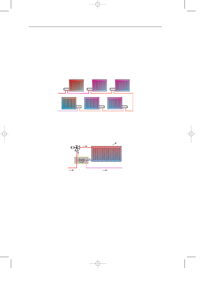
5 . O N E - P I P E D I S T R I B U T I O N
39
5. One-pipe distribution
5.1 General
In a one-pipe distribution, radiators are connected in series. Each radiator valve splits the
flow into one part being bypassed and one part going through the radiator. The water
leaving one radiator valve enters the next one as shown in Fig 5.1.
If the entire loop flow passes through the radiators, isolation of a single radiator will stop
circulation in all radiators in the loop. This is why the bypass is installed at each one-pipe
valve as shown in Fig 5.2.
P
= Heat emission in W.
q
L
= Loop flow in l/h.
λ
q
L
= Water flow in the radiator.
t
1
= Inlet water temperature.
t
r
= Outlet water temperature from the radiator.
t
2
= Inlet water temperature for the next radiator.
The differential pressure created by the restriction in the bypass generates the flow
through the radiator. This flow is limited by the thermostatic valve.
Fig 5.1. Radiators with one-pipe distribution.
Fig 5.2. A bypass diverts part of the loop flow.
q
L
λ
.
q
L
t
1
t
r
t
2
q
L
P
TA-Handbok 3 (GB) 03-04-24 14.25 Sida 39

B A L A N C I N G O F R A D I A T O R S Y S T E M S
40
If P is the heat output of the radiator, the supply water temperature t
2
for the next radiator
is calculated as follows:
The water temperature in the loop decreases after each radiator; this must be taken into
account when choosing nominal radiator power.
5.1.1 ADVANTAGES
– Reduced pipe lengths.
When radiators can be spread out throughout the entire loop, the pipe length can be
reduced by up to 50%. This also reduces heat emission from pipes, which cannot be
controlled by thermostatic valves.
– Lower labour cost.
Installation is very fast when pipes are laid out in loops. Many accessories such as tees and
elbows are eliminated. The labour saving compared with a traditional two-pipe installation
can exceed 40%.
– More reliable installation.
Pipes are usually made of copper or soft steel and protected by plastic. The use of cross-
linked polyethylene tubes is also becoming quite common. All of these pipes are well
protected against corrosion and can be laid in a single operation without any connection in
the concrete, making the installation more reliable in the long term.
– Distribution with practically constant flow.
Since the flow in the loop is almost constant, the various loops are not interactive.
– The pipes emission can be deducted from the heat losses to calculate the radiators.
This advantage will be discussed in section 5.1.3.
0.86 x P
cc cci
q
L
t
2
= t
1
–
TA-Handbok 3 (GB) 03-04-24 14.25 Sida 40

5 . O N E - P I P E D I S T R I B U T I O N
41
5.1.2 DISADVANTAGES AND LIMITATIONS
– Increased total surface of heating elements.
The radiators at the end of the loop must be oversized to compensate for the lower water
temperature. The total surface of heating elements installed in a one-pipe distribution is
therefore sometimes greater than in a two-pipe distribution system.
– The return water temperature may be higher than in two-pipe systems.
One-pipe loops have a practically constant flow. When all thermostatic valves are closed,
the temperature of the return water is equal to the supply temperature. District heating
companies require the lowest possible return temperatures, and therefore do not like one-
pipe distributions. This comment should be kept in proportion, since the supply water
temperature normally depends on outside conditions. In this case it is only accidental if
most thermostatic valves are closed. However, it frequently happens that one-pipe loops
work with a lower
∆
T than two-pipe loops in order to reduce heating surfaces to be
installed. In this case the return is effectively warmer.
– Interactivity between radiators in the loop.
Let us consider a loop with four radiators. When closing the first two, the water temper-
ature on the last two will increase. The thermostatic valves on these radiators then have
to compensate for a potential increase in emission in the region of 10 to 15%. However
closing the last two radiators affects the loop flow by reducing the power of the first two
radiators by around 3 to 5%. These interactivity phenomena do not create a real problem
and depend on the
∆
T used in the loop and the proportion of the loop flow absorbed by
the radiators.
When the flow in the radiators is not balanced, the power emitted by the first radiators
when the installation starts up may be higher than planned. In this case, the supply water
temperature to the last radiators in the loop is too low to be able to supply the required
power. It is therefore important to balance the loop by providing the necessary flow to
each radiator.
TA-Handbok 3 (GB) 03-04-24 14.25 Sida 41

B A L A N C I N G O F R A D I A T O R S Y S T E M S
42
5.1.3 EMISSION FROM PIPES
Connecting pipes emit heat in addition to heat emitted by radiators. This emission is
normally ignored when selecting heating elements, but must be considered in calculating
the water temperature drop in the loop.
Emission from pipes in the environment depends on the water temperature, the pipe
diameter, its degree of insulation, and the pipe location (visible, cast in concrete, etc.).
For a water temperature of 80 °C and a room temperature of 20 °C, the heat losses
of a visible plastic tube are of 30 W/m (d
i
= 10 mm) and 60 W/m for d
i
= 20 mm. For a
diameter d
i
between 10 and 20 mm, the heat emitted per metre from a visible pipe can be
estimated using the following formula:
P
=
Heat losses in W/m.
t
s
=
The supply water temperature.
t
i
=
The room temperature.
d
i
=
Pipe diameter (mm).
If each radiator is connected with 6 metres of pipe (d
i
= 15 mm), emission from pipes at
80 °C would theoretically reduce the required heat output for each radiator by 270 W.
This relative effect is quite significant for small radiators, but is often ignored in the
calculations. Some well-insulated installations provide adequate heating throughout the
entire heating season with all radiators closed as the pipes alone provide sufficient
heat. In some countries, all connecting pipes, even those inside the apartment, must be
thoroughly insulated. This gives better control of the heating power.
When a thermostatic valve closes, emission from the pipe continues and may make
the room too warm. However this is limited since the water temperature supply depends
on outside conditions. In some very well-insulated installations, a control valve is placed
in the loop and isolates this loop when the temperature in a reference room exceeds a
limiting value, for example 22 °C.
The problem of uncontrolled emission from pipes is not inherent to the one-pipe
system. In a two-pipe distribution as shown in Fig 5.3, this emission is even increased by
the presence of two distribution pipes instead of one.
d
i
c ci
15
P = (t
s
– t
i
)
×
TA-Handbok 3 (GB) 03-04-24 14.25 Sida 42
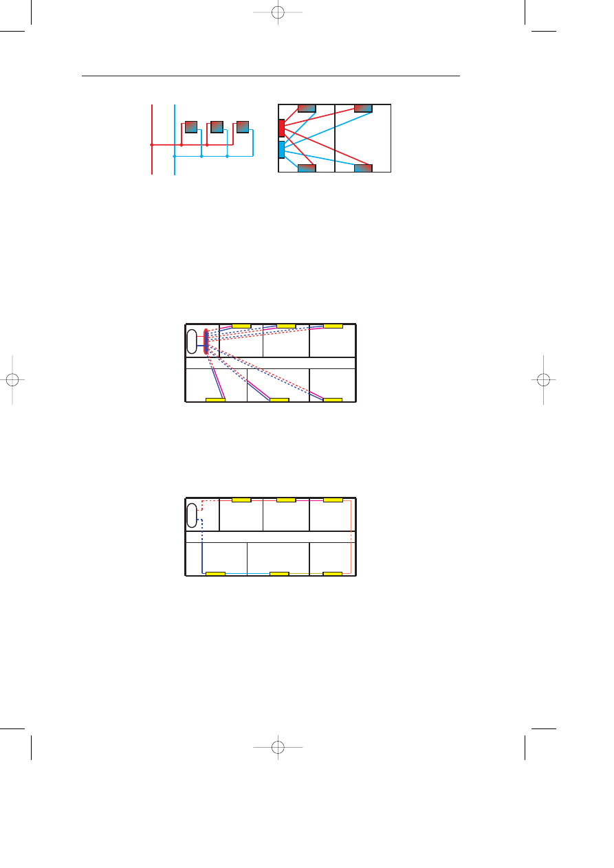
5 . O N E - P I P E D I S T R I B U T I O N
43
When each radiator is individually connected to the distributors, the closure of a thermo-
static valve stops the pipe emission into the room and into the adjacent room where this
action is in fact a disturbance.
In a two-pipe distribution as shown in Fig 5.4, the emission of pipes in a room is
variable and depends mainly on the room temperature control in other rooms. For this
reason, the pipe emission cannot be deducted from the heat losses when calculating the
radiators. However, pipe emission must be calculated to determine the real supply water
temperature for each radiator.
The opposite is true for a one-pipe distribution (Fig 5.5); the pipes emission does not
influence the function of the radiators in practice. Consequently, this emission can be
deducted from the heat losses to calculate the radiators.
Fig 5.4. In a two-pipe system, the pipes emission in a room
depends mainly on other rooms.
100 to 600 W
100 to 300 W
85
°
C
1000 W - 85
°
C - 43 l/h
or
777 W - 73
°
C - 43 l/h
?
Fig 5.5. In a one-pipe distribution the pipes emission can be deducted
from the heat losses to calculate the radiators.
Fig 5.3. Emission from pipes in a two-pipe distribution.
a
b
TA-Handbok 3 (GB) 03-04-24 14.25 Sida 43
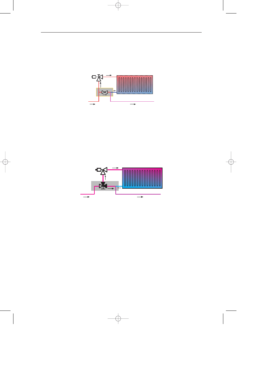
B A L A N C I N G O F R A D I A T O R S Y S T E M S
44
5.2 One-pipe valves
5.2.1 CONSTANT BYPASS – VARIABLE KV
Several methods of installation are possible.
In the case shown in Fig 5.6, the resistance of the bypass is fixed and the proportion of
the loop flow passing through the radiator is obtained by reducing the Kv
max
of the
thermostatic valve. For a small radiator, most of the flow passes through the bypass, and
the pressure loss in the bypass may be unnecessarily high. In this case, the Kv of the
bypass should be increased, and therefore a variable bypass valve should be used.
5.2.2 VARIABLE BYPASS – CONSTANT KV
In Fig 5.7, a three-way diverting valve distributes flows between the radiator and the
bypass at constant total Kv. The pressure loss across the module only depends on the flow
in the loop. The adjustment of the flow through a radiator, with the bypass three-way
valve, has no influence on the flow loop.
Fig 5.7. Distributor with variable bypass.
t
1
t
2
t
r
λ
.
q
L
q
L
q
Fig 5.6. Distributor with fixed bypass.
q
L
λ
.
q
L
t
1
t
r
t
2
q
L
TA-Handbok 3 (GB) 03-04-24 14.25 Sida 44
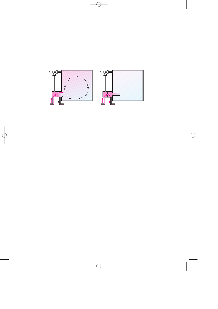
5 . O N E - P I P E D I S T R I B U T I O N
45
5.2.3 PROTECTION AGAINST DOUBLE CIRCULATION
When the thermostatic valve closes, the bottom of the radiator remains in direct contact
with the hot water pipe. This can create double circulation in the return orifice (Fig 5.8a)
with uncontrollable emission from the radiator. This is why a tube should be inserted in
the radiator as shown in Fig 5.8b, in order to prevent the double circulation phenomenon.
This inserted tube cannot be placed on all radiators.
5.3 Proportion of the loop flow in the radiator (
λ
coefficient)
5.3.1 50% FLOW IN THE RADIATOR (
λ
= 0.5)
In early versions of the one-pipe system, 50% of the loop flow was designed for the
radiator. This magic figure results from the fact that the temperature t
2
of the water supply
to the next radiator is equal to the arithmetic mean temperature of the previous radiator.
As we saw under Fig 5.2, t
2
is very easily calculated. Based on the average temperature of
the radiator, it was then possible to calculate the nominal power to be installed to obtain
the necessary emission.
The high overflow in the radiator was considered to improve its emission, and thus
make it possible to reduce heating surface areas to be installed. This is not always true as
too high a velocity in the inlet creates a suction effect. Cold water in the bottom of the
radiator is mixed with the hot water in the inlet decreasing, to a certain extent, the heat
output. However, passing 50% of a loop flow of 500 l/h in a 250 W radiator is equivalent
to 23 times its nominal flow. Reducing the flow using the thermostatic valve has practically
no effect on emission for 96% (22/23) of its nominal lift. Therefore the valve usually works
near its closed position, with the risk of being inefficient.
Moreover, when a thermostatic valve closes, the entire flow must pass through the
bypass. Therefore the flow in the bypass is doubled, and the pressure loss is quadrupled.
This high pressure loss affects the total flow and the emission from the radiators in the
loop. To ensure that this will not happen, a lower proportion of the flow can be taken in
the radiator. Flow variations in the bypass are then lower and the loop flow is more stable.
Fig 5.8. With the thermostatic valve closed, double circulation can take place in the radiator
return connection. An inserted tube can practically eliminate this phenomenon.
a
b
TA-Handbok 3 (GB) 03-04-24 14.25 Sida 45

B A L A N C I N G O F R A D I A T O R S Y S T E M S
46
5.3.2 CHOICE OF ANOTHER FLOW IN THE RADIATOR
For loop flows of up to 200 l/h, the TA-RSD 801 one-pipe valve has a Kv = 1.2 and the
flow in the radiator can be adjusted from 0 to 50% of the loop flow.
For loop flows of more than 200 l/h, the Kv of the TA-RSD 831 is 2.8 and the flow
in the radiator is adjustable from 0 to 20% of the loop flow.
In both cases, the Kv of the TA-RSD one-pipe valve is independent of the flow
proportion chosen in the radiator.
In order to estimate its required nominal power, the maximum possible flow is
generally assumed in the radiator with a minimum value of 10K for the
∆
T.
The radiator is selected on this basis but, since the choice is limited, its real nominal
power is generally higher than the calculated power. The real flow necessary to obtain the
calculated heating power is then determined.
Example: In a 400 l/h loop, a radiator is supplied at a water temperature ts of 82 °C
and must emit 850 W into an environment of 20 °C.
Preliminary calculation: 20% of 400 l/h = 80 l/h. For a
∆
T of 10K, the flow must
be 0.86 x 850/10 = 73 l/h. The lowest of these two flows is used, namely 73 l/h
and the
∆
T is therefore 10K.
Using the diagram in Fig A1 (in appendix A), it is found that the nominal 75/65 over-
sizing factor of the radiator is 0.84 (Join t
s
– t
i
= 82 – 20 = 62 to t
r
– t
i
= 72 – 20 = 52).
The nominal power 75/65 of the radiator to be installed is therefore 850
×
0.84 = 716 W.
Final calculation: The real nominal power of the chosen radiator is 935 W. What flow
should be adjusted at the radiator?
The oversizing factor Sp is therefore 935/850 = 1.1.
Using Fig A1 again, join (t
s
- t
i
) = (82 – 20) = 62 to Sp = 1.1 to get t
r
– t
i
= 34.5
therefore t
r
= 54.5.
The required
∆
T is therefore 82 – 54.5 = 27.5K and the flow q = 0.86
×
850/27.5 =
26.6 l/h, namely 7% of the loop flow.
When an installation is being renovated, the nominal power of radiators is given. The flow
in the radiator is therefore determined based on the diagram in Fig A1 directly, using the
oversizing factor and the supply water temperature. In some new buildings, for aesthetic
reasons, all radiators are identical and the correct power has to be obtained by appropriate
adjustment of the flow to each radiator.
TA-Handbok 3 (GB) 03-04-24 14.25 Sida 46

5 . O N E - P I P E D I S T R I B U T I O N
47
5.4 The loop flow
In theory, it is better to use the highest possible loop flow. This reduces the temperature
drop in the loop and the required heating surface area for the last radiators. Moreover,
when thermostatic valves close on the first radiators in the loop, there is not a high increase
in the water temperature for the last radiators.
In practice, the loop flow is limited by the available differential pressure in relation
to the pipe size, the number of radiators etc.
The total loop power and the supply water temperature are the predominant factors
to determine the realistic value for the loop flow (see section 5.4.1). In some cases, when
λ
max
= 0.2, a large radiator in the loop can be the predominant factor (see section 5.4.2).
5.4.1 BASED ON A GIVEN
∆
T
The loop flow is a result of the chosen
∆
T and the sum
Σ
P of powers, emitted by radiators
in the loop, according to the following formula:
q
L
=
Loop flow in l/h.
Σ
P =
Sum of the required heat output in W of the radiators in the loop.
∆
T
L
= Temperature drop in the loop (K).
Obviously, the allowable temperature drop reduces with the supply water temperature. The
temperature drop in the loop is normally given by
∆
T
L
< 0.25
×
(t
s
– 20). Substituting this
value in the previous formula gives an estimation of the lowest realistic loop flow:
Example: If
Σ
P = 4 000 W and t
s
= 80 °C, q
L
> 230 l/h.
5.4.2 BASED ON THE LARGEST RADIATOR IN THE LOOP (WHEN
λ
max
= 0.2)
The largest radiator in the loop, PM, requires a minimum flow to avoid unreasonable
oversizing. Using an effectiveness
φ
= 0,43 =
∆
T
R
/(t
s
– t
i
) for example: q
R
= 0,2
×
q
L
=
P
M
×
0,86/
∆
T
R
and
5.4.3 FINAL CHOICE OF THE LOOP FLOW
The highest water flow from the two methods of calculation is chosen.
10
×
P
M
c ci
t
s
– 20
q
L
=
3.44
× ∑
P
c ci
(t
s
– 20)
q
L
>
0.86
× ∑
P
c ci
∆
T
L
q
L
>
TA-Handbok 3 (GB) 03-04-24 14.25 Sida 47
B A L A N C I N G O F R A D I A T O R S Y S T E M S
48
5.5 Pressure losses in the loop
For a flow of 300 l/h in a pipe with an inside diameter of 14 mm, the pressure loss for water
at 20 °C is 317 Pa/m (32 mm/m) and 278 Pa/m at 70 °C (Nomogram B1 in Appendix B)
One-pipe valves may be converted into equivalent metres of pipe as shown in table
5.1 below.
That means, for instance, that a valve of Kv = 2.8 with two elbows has a pressure drop
equivalent to 4.72 metres of pipe (di = 14 mm).
Table 5.1. Metres of equivalent pipe for valves with Kv =1.2 and 2.8.
Equivalence for a single elbow. Water temperature 70 °C.
d
i
mm
10
11
12
13
14
15
16
17
18
Kv=1.2
3.79
6.23
9.80
14.87
21.88
Kv=2.8
0.69
1.14
1.80
2.73
4.02
5.76
8.06
11.05
14.88
1 elbow
0.24
0.26
0.29
0.32
0.35
0.39
0.42
0.45
0.48
TA-Handbok 3 (GB) 03-04-24 14.25 Sida 48
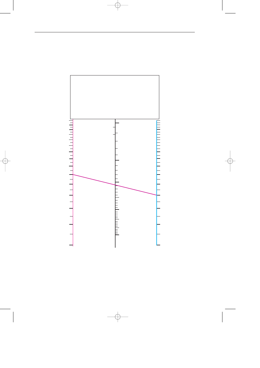
A P P E N D I C E S
49
Appendices
A. Calculation of radiators in several conditions
Fig A1. The power of a radiator not working
in nominal condition (n = 1.3).
20
30
40
50
60
70
t
s
- t
i
t
r
- t
i
75/65
P
n
/ P
0.5
1.0
1.5
2.0
3.0
4.0
20
30
40
50
60
70
t
s
= Supply water temperature
t
r
= Return water temperature
t
i
= Romm temperature required
P = Heat output required
P
n
= Nominal heat output of radiator
Nominal conditions
t
sn
= 90 °C
t
rn
= 70 °C
t
in
= 20 °C
t
sn
= 80 °C
t
rn
= 60 °C
t
in
= 20 °C
TA-Handbok 3 (GB) 03-04-24 14.25 Sida 49
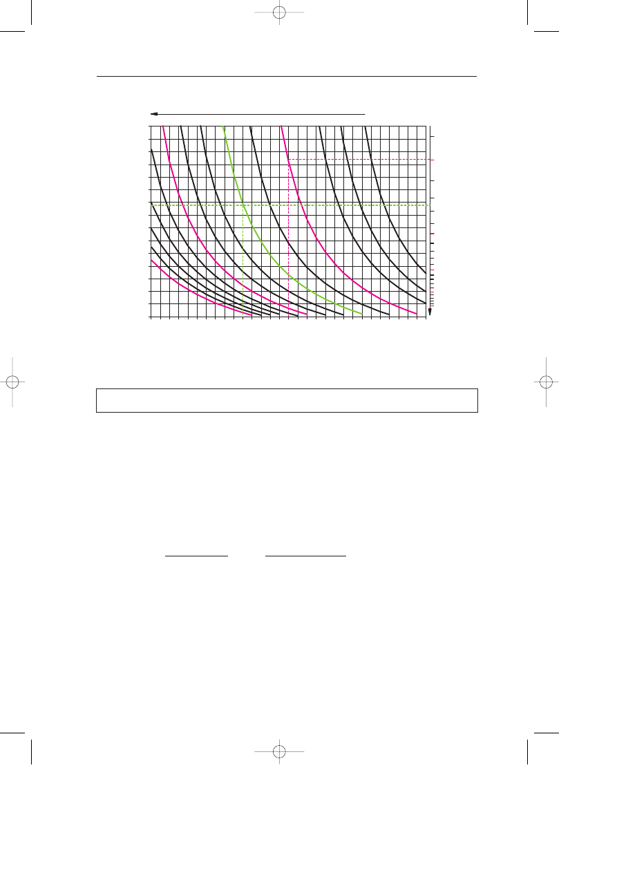
B A L A N C I N G O F R A D I A T O R S Y S T E M S
50
Examples: (using Fig A1 and nominal conditions 75/65)
1. The heat losses in a room are 1000 W. t
s
= 60 °C and t
r
= 50 °C. What nominal radiator
power should be installed if the required room temperature is 20 °C?
Join t
s
– t
i
= 60 – 20 = 40 to point t
r
– t
i
= 50 – 20 = 30, to find P
n
/P = 1.6. We therefore
need to install a 1000
×
1.6 = 1600 W radiator (75/65 conditions) to obtain 1000 W
(60/50 conditions).
The required flow is P
×
0.86/
∆
T
c
= 1000
×
0.86/10 = 86 l/h.
The following formula can also be used:
2. 750 W must be transferred with a radiator supplied at 70 °C. The flow is 43 l/h. What
nominal capacity should be installed if the room temperature to be obtained is 22 °C?
∆
T = 0.86 x 750/43 = 15K therefore t
r
= t
s
–
∆
T = 70 – 15 = 55 °C. Join t
s
– t
i
=
70 – 22 = 48 to point t
r
– t
i
= 55 – 22 = 33, to find P
n
/P = 1,33. We therefore have to
install a 750
×
1.33 = 948 W radiator.
Fig A2. Water flow in l/h per 1000 W is a function of the oversizing factor Sp = P
n
/P and
the supply water temperature t
s
(nominal condition t
sn
= 75 °C, t
rn
= 65 °C).
t
s
- ti)
W
a
ter flow in l/h per 1000 W output
25
30
35
40
45
50
55
60
65
70
75
80
85
90
95
100
40
45
50
55
60
65
70
0.8
0.9
1
1.1
1.2
1.3
1.4
1.5
SP = P
n
/P
30
20
25
15
14
13
12
11
10
9
∆
T
2475
icfff cccccci
2475
icfff cccccci
(t
s
– t
i
) (t
r
– t
i
)
(60 – 20) (50 – 20)
SP =
(
)
n/2
=
(
)
1.33/2
= 1.6
TA-Handbok 3 (GB) 03-04-24 14.25 Sida 50

A P P E N D I C E S
51
3. A radiator has a nominal capacity of 1250 W, whereas losses are only 1000 W. The
water supply temperature is 80 °C and the room temperature is 20 °C. What should
the water flow be to compensate for this oversizing?
Join t
s
– t
i
= 80 – 20 = 60 to P
n
/P = 1250/1000 = 1,25, to find t
r
– t
i
= 29. Therefore
t
r
= 29 + 20 = 49 °C.
The water temperature drop must be t
r
– t
s
= 80 – 49 = 31K 31K and the water flow to
be set 0.86
×
1000/31 = 28 l/h, whereas the nominal flow through a 1250 W radiator is
0.86
×
1250/10 = 108 l/h.
For computer, following formula can also be used:
This formula has been translated in the graph of figure A2.
4. On a radiator with a nominal capacity of 1000 W (75/65), we measure a water inlet
temperature ts of 55 °C and a return temperature t
r
of 50 °C. The room temperature
t
i
is 22.5 °C for an outdoor temperature t
e
= 3 °C.
4.1 What is the present heat transfer of the radiator?
Join (t
s
– t
i
) = 55 – 22.5 = 32.5 °C to (t
r
– t
i
) = 50 – 22.5 = 27.5 °C.
Then P
n
/P = 1.94. Therefore P = 1000/1.94 = 515 W.
4.2 What is the present flow compared with the nominal flow?
Nominal flow = 0.86 P
n
/
∆
T
n
= 0.86
×
1000/10 = 86 l/h.
Present real flow = 0.86
×
515/(55 – 50) = 88.6 l/h.
4.3 What would the heat losses be for t
e
= 3 °C if the room temperature was 20 °C?
Present heat losses = 515 = k (t
i
– t
e
) = k (22.5 – 3) therefore k = 26.4.
Losses for t
i
= 20 °C ger k (20 – 3) = 26.4 (20 – 3) = 449 W.
4.4 What should the return temperature t
r
and the water flow q be, to obtain a room
temperature of 20 °C?
For t
i
= 20 °C, P
n
/P = 1000/449 = 2.23. Join (t
s
– t
i
) = (55 – 20) = 35 to P
n
/P =
2.23. To find (t
r
– t
i
) = (t
r
– 20) = 20.6 °C.
Therefore t
r
= 20 + 20.6 = 40.6 °C and
∆
T = 55 – 40.6 = 14.4K.
To obtain these conditions, the water flow must be: 0.86 P/
∆
T = 0.86
×
449/14.4
= 3.2 l/h.
4.5 What nominal radiator capacity would have been necessary to work under nominal
conditions, if the outdoor design temperature t
ec
= –10 °C?
Losses at t
ec
= – 10 °C: k (20 – (–10)) = 26.4
×
30 = 792 W.
The installed radiator capacity should have been 792 W with a flow of 0.86
×
792/10 = 68 l/h.
0.86
×
P
icfff cvvvvvvvvvviccccci
0.86
×
1000
icfff i nnnnnnnnnnnnnnncccccci
q =
= = 48 l/h
2475
ff cc cci
2475
icfvffiicci
(t
s
– t
i
)
(80 – 20)
(t
s
– t
i
) –
×
S
Pn
–2/n
(80 – 20) –
×
1.25
– 2/1.33
TA-Handbok 3 (GB) 03-04-24 14.25 Sida 51
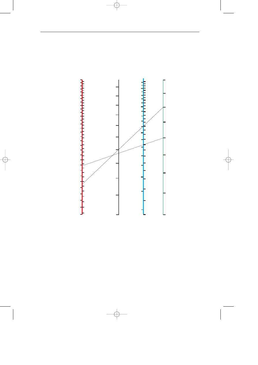
B A L A N C I N G O F R A D I A T O R S Y S T E M S
52
B. Pressure losses in pipes.
0.40
0.50
0.60
0.70
0.80
10
11
12
13
14
15
16
17
18
0.050
0.100
0.150
0.200
100
200
300
400
500
600
700
800
∆
p
v
q
d
i
70
°
C
50
°
C
m/s
l/s
l/h
mm
Pa/m
200
500
250
300
350
400
450
600
550
500
450
400
350
300
250
Fig B1a. Pressure losses in pipes with roughness less than 0.0045
(smooth steel, copper, polyethylene, etc.)- di is the inside diameter of the pipe in mm.
TA-Handbok 3 (GB) 03-04-24 14.25 Sida 52
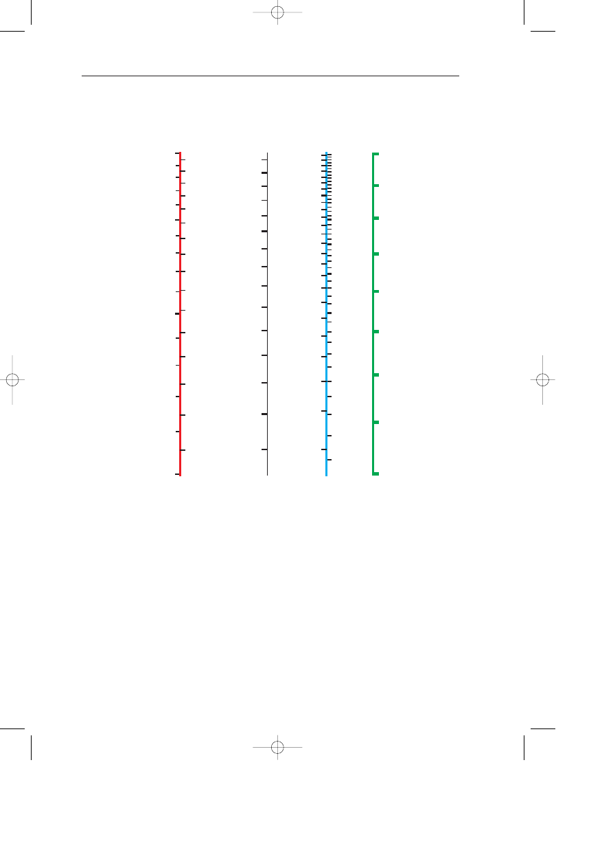
A P P E N D I C E S
53
Fig B1b. Pressure losses in pipes with roughness less than 0.0045
(smooth steel, copper, polyethylene, etc.)- di is the inside diameter of the pipe in mm.
10
1
12
13
14
15
16
17
18
∆
p
v
q
d
i
70
°
C
5
0
°
C
m/s
l/s
l/h
mm
Pa/m
50
100
150
200
250
300
350
400
450
0.02
0.04
0.06
0.08
0.10
0.12
0.20
0.30
0.40
0.50
200
150
50
100
100
150
200
TA-Handbok 3 (GB) 03-04-24 14.25 Sida 53
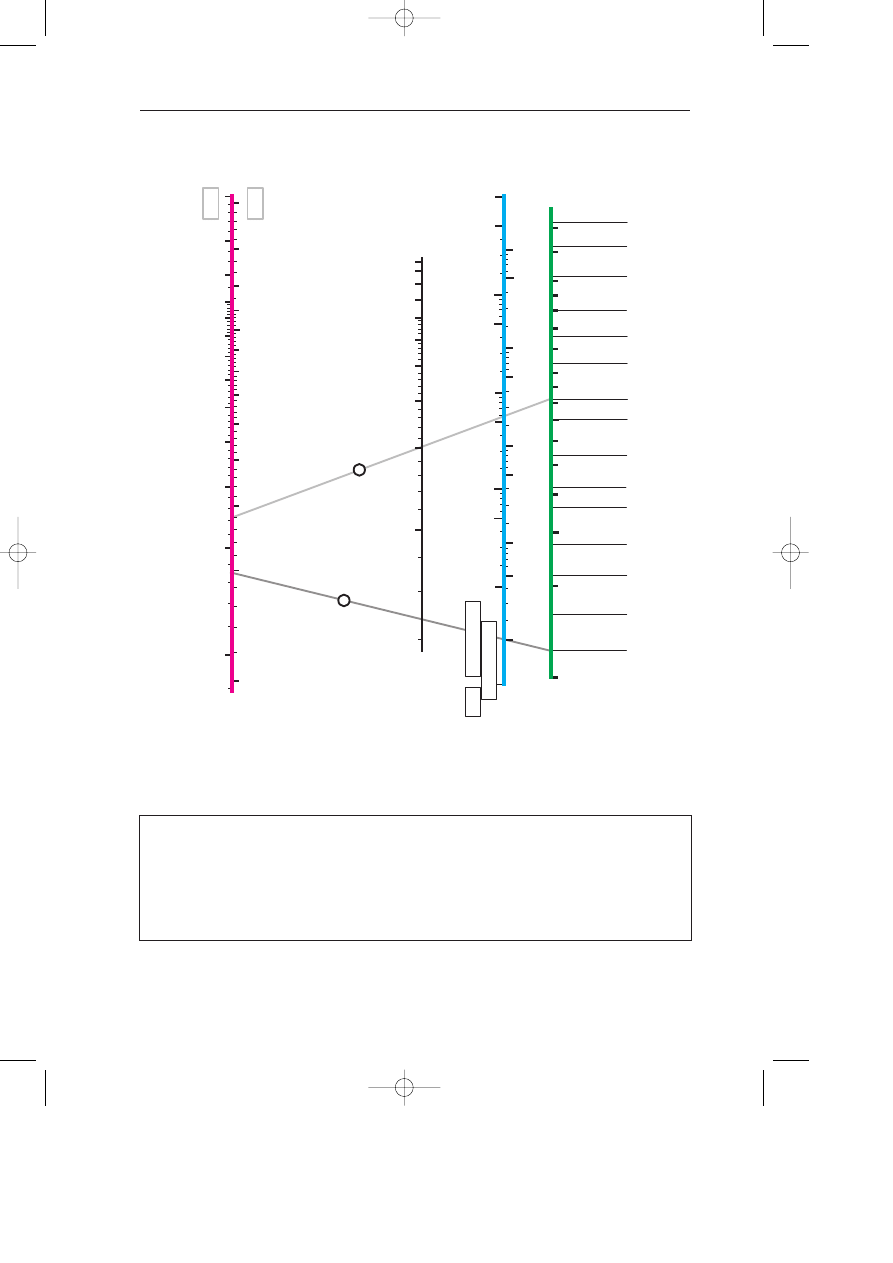
B A L A N C I N G O F R A D I A T O R S Y S T E M S
54
Example 1: Pipe DN80 (di = 82.5 mm) and water flow 20 m
3
/h: Velocity = 1 m/s
and
∆
p = 140 Pa/m (at 20 °C).
Example 2: Pipe DN10 (di = 12.5 mm) and water flow 0.1 m
3
/h: Reynolds number
being below 3500, this nomogram is not applicable in this case, as it was established
for turbulent conditions.
Fig B2. Pressure drops and velocities (pipes with a roughness of 0.05 mm)
for water at 20 and 70 °C.
1
2
∆
p
Pa/m
750
mm
v
m/s
q
di
l/s
m
3
/h
70
°
C
20
°
C - Re < 3500
5
°
C - Re < 3500
50
100
150
200
250
300
350
400
450
500
600
50
100
150
200
250
300
350
400
450
500
600
750
70
°
C
20
°
C
5.0
4.0
0.2
0.3
0.4
0.5
1.0
1.5
2.0
2.5
3.0
500
0.1
0.5
1
5
10
50
100
1000
0.1
0.5
1
5
10
50
100
500
DN300
300
10
20
30
40
50
60
70
80
90
100
120
140
160
180
200
250
DN10
DN15
DN20
DN25
DN32
DN40
DN50
DN65
DN80
DN100
DN125
DN150
DN200
DN250
TA-Handbok 3 (GB) 03-04-24 14.25 Sida 54

TA-Handbok 3 (GB) 03-04-24 14.25 Sida 55

M-010
2003.04
Certification of Registration
Number 2125 and 2125 M
Certified by SP
Q
U
A
L
IT
Y
AN
D ENVIRONMEN
T
SY
S
T
E
M
TO
UR
& AN
DERSSO
N
AB
Great Britain
Tour & Andersson Ltd,
Barratt House, 668 Hitchin Road,
Stopsley Luton, Bedfordshire, LU2 7XH,
U.K.
Tel: +44 (0)1582 876 232.
Fax: +44 (0)1582 488 678.
www.tourandersson.com
Sweden
Tour & Andersson AB
Norra Gubberogatan 32,
Box 6281, SE-400 60 Göteborg
Tel +46 31 338 73 30.
Telefax +46 31 338 73 49
www.tourandersson.com
Australia
Tour & Andersson
PO Box 154
HIGHETT VIC 3190
Tel +61 3 9553 3366.
Telefax +61 3 9553 3733
www.tourandersson.com
Singapore
Tour & Andersson Pte Ltd
171 Chin Swee Road, #05-01 San
Centre
SINGAPORE 169877
Tel +65 65 32 06 26.
Telefax +65 65 32 29 19
www.tourandersson.com
TA-Handbok 3 (GB) 03-04-24 14.25 Sida 56
Wyszukiwarka
Podobne podstrony:
Harmonogram 2 (KiP), Rozliczenie czasu pracy w równoważnym systemie czasu pracy - listopad 2006
09 Równowaga systemu ekonomicznego Inflacja
odp, Politechnika Łódzka Elektrotechnika, magisterskie, 1 sem, systemy el-en, kolo
System el-en. 13 14 1, Prywatne, EN-DI semestr 4, Elektroenergetyka, wykład + ćwiczenia
sprawko Malczewski, Politechnika Łódzka Elektrotechnika, magisterskie, 1 sem, systemy el-en, Systemy
08 Równowaga systemu ekonomicznego Rynek pracy
07 Równowaga systemu ekonomicznego
DARWIN Connection System SmartWireMN03407001Z EN
ZESZYT 2 Rownoważenie przepływów w układach rozdzielchych
Arypiprazol (Abilify) nowy lek przeciwpsychotyczny, pierwszy lek stabilizujący równowagę systemu dop
System el en 11 12 1
BMW 03 00 Nav system manual en
Systemy PV współpr z siecią en folie
Dokumentacja systemu zarządzania jakością w oparciu o normę PN EN ISO?01 2009 (2)
Metoda 6 Sigma w systemie zarządzania laboratorium według normy PN EN ISO IEC 17025 2005
Praca w systemie równoważnym a karmienie piersią, Prawna ochrona pracy, Kadry i Płace(1)
EN ISO 19011cd, WZR UG, VI semestr, Systemy zarządzania środowiskowego - dr Richert Maria
Bezpieczenstwo w systemach sterowania wedlug normy ISO EN 13849 1 (1)
więcej podobnych podstron