
Calculus of Variations and Optimal Control

iii
Preface
This pamphlet on calculus of variations and optimal control theory contains the most impor-
tant results in the subject, treated largely in order of urgency. Familiarity with linear algebra and
real analysis are assumed. It is desirable, although not mandatory, that the reader has also had a
course on differential equations. I would greatly appreciate receiving information about any errors
noticed by the readers. I am thankful to Dr. Sara Maad from the University of Virginia, U.S.A.,
for several useful discussions.
Amol Sasane
6 September, 2004.

Course description of MA305:
Control Theory
Lecturer: Dr. Amol
Sasane
Overview
This a high level methods course centred on the establishment of a calculus appropriate to
optimisation problems in which the variable quantity is a function or curve. Such a curve might
describe the evolution
over continuous time of the state of a dynamical system. This is typical of models of consumption
or production in economics and financial mathematics (and for models in many other disciplines
such as engineering and physics).
The emphasis of the course is on calculations, but there is also some theory.
Aims
The aim of this course is to introduce students to the types of problems encountered in optimal
control, to provide techniques to analyse and solve these problems, and to provide examples of
where these techniques are used in practice.
Learning Outcomes
After having followed this course, students should
* have knowledge and understanding of important definitions, concepts and results,
and how to apply these in different situations;
* have knowledge of basic techniques and methodologies in the topics covered below;
* have a basic understanding of the theoretical aspects of the concepts and methodologies
covered;
* be able to understand new situations and definitions;
* be able to think critically and with sufficient mathematical rigour;
* be able to express arguments clearly and precisely.
The course will cover the following content:
1. Examples of Optimal Control Problems.
2. Normed Linear Spaces and Calculus of Variations.
3. Euler-Lagrange Equation.
4. Optimal Control Problems with Unconstrained Controls.
5. The Hamiltonian and Pontryagin Minimum Principle.
6. Constraint on the state at final time. Controllability.
7. Optimality Principle and Bellman's Equation.

Contents
1
Introduction
1
1.1
Control theory . . . . . . . . . . . . . . . . . . . . . . . . . . . . . . . . . . . . . .
1
1.2
Objects of study in control theory
. . . . . . . . . . . . . . . . . . . . . . . . . . .
1
1.3
Questions in control theory . . . . . . . . . . . . . . . . . . . . . . . . . . . . . . .
3
1.4
Appendix: systems of differential equations and e
tA
. . . . . . . . . . . . . . . . .
4
2
The optimal control problem
9
2.1
Introduction . . . . . . . . . . . . . . . . . . . . . . . . . . . . . . . . . . . . . . . .
9
2.2
Examples of optimal control problems . . . . . . . . . . . . . . . . . . . . . . . . .
9
2.3
Functionals . . . . . . . . . . . . . . . . . . . . . . . . . . . . . . . . . . . . . . . .
12
2.4
The general form of the basic optimal control problem . . . . . . . . . . . . . . . .
13
3
Calculus of variations
15
3.1
Introduction . . . . . . . . . . . . . . . . . . . . . . . . . . . . . . . . . . . . . . . .
15
3.2
The brachistochrone problem . . . . . . . . . . . . . . . . . . . . . . . . . . . . . .
16
3.3
Calculus of variations versus extremum problems of functions of n real variables
.
17
3.4
Calculus in function spaces and beyond
. . . . . . . . . . . . . . . . . . . . . . . .
18
3.5
The simplest variational problem. Euler-Lagrange equation . . . . . . . . . . . . .
24
3.6
Free boundary conditions . . . . . . . . . . . . . . . . . . . . . . . . . . . . . . . .
31
3.7
Generalization
. . . . . . . . . . . . . . . . . . . . . . . . . . . . . . . . . . . . . .
33
4
Optimal control
35
4.1
The simplest optimal control problem . . . . . . . . . . . . . . . . . . . . . . . . .
35
4.2
The Hamiltonian and Pontryagin minimum principle . . . . . . . . . . . . . . . . .
38
4.3
Generalization to vector inputs and states . . . . . . . . . . . . . . . . . . . . . . .
40

vi
Contents
4.4
Constraint on the state at final time. Controllability . . . . . . . . . . . . . . . . .
43
5
Optimality principle and Bellman’s equation
47
5.1
The optimality principle . . . . . . . . . . . . . . . . . . . . . . . . . . . . . . . . .
47
5.2
Bellman’s equation . . . . . . . . . . . . . . . . . . . . . . . . . . . . . . . . . . . .
49
Bibliography
55
Index
57

Chapter 1
Introduction
1.1
Control theory
Control theory is application-oriented mathematics that deals with the basic principles underlying
the analysis and design of (control) systems. Systems can be engineering systems (air conditioner,
aircraft, CD player etcetera), economic systems, biological systems and so on. To control means
that one has to influence the behaviour of the system in a desirable way: for example, in the case
of an air conditioner, the aim is to control the temperature of a room and maintain it at a desired
level, while in the case of an aircraft, we wish to control its altitude at each point of time so that
it follows a desired trajectory.
1.2
Objects of study in control theory
The basic objects of study are underdetermined differential equations. This means that there is
some freeness in the choice of the variables satisfying the differential equation. An example of
an underdetermined algebraic equation is x + u = 10, where x, u are positive integers. There is
freedom in choosing, say u, and once u is chosen, then x is uniquely determined. In the same
manner, consider the differential equation
dx
dt
(t) = f (x(t), u(t)), x(t
i
) = x
i
, t
≥ t
i
,
(1.1)
1
2
Chapter 1. Introduction
x(t)
∈ R
n
, u(t)
∈ R
m
. So written out, equation (1.1) is the set of equations
dx
1
dt
(t)
=
f
1
(x
1
(t), . . . , x
n
(t), u
1
(t), . . . , u
m
(t)), x
1
(t
i
) = x
i,1
..
.
dx
n
dt
(t)
=
f
n
(x
1
(t), . . . , x
n
(t), u
1
(t), . . . , u
m
(t)), x
n
(t
i
) = x
i,n
,
where f
1
, . . . , f
n
denote the components of f . In (1.1), u is the free variable, called the input, which
is usually assumed to be piecewise continuous
1
. Let the class of
R
m
-valued piecewise continuous
functions be denoted by
U. Under some regularity conditions on the function f : R
n
× R
m
→ R
n
,
there exists a unique solution to the differential equation (1.1) for every initial condition x
i
∈ R
n
and every piecewise continuous input u:
Theorem 1.2.1
Suppose that f is continuous in both variables. If there exist K > 0, r > 0 and
t
f
> t
i
such that
f(x
2
, u(t))
− f(x
1
, u(t))
≤ Kx
2
− x
1
(1.2)
for all x
1
, x
2
∈ B(x
i
, r) =
{x ∈ R
n
| x − x
i
≤ r} and for all t ∈ [t
i
, t
f
], then (1.2) has a
unique solution x(
·) in the interval [t
i
, t
m
], for some t
m
> t
i
. Furthermore, this solution depends
continuously on x
i
for fixed t and u.
Remarks.
1. Continuous dependence on the initial condition is very important, since some inaccuracy
is always present in practical situations. We need to know that if the initial conditions are
slightly changed, the solution of the differential equation will change only slightly. Otherwise,
slight inaccuracies could yield very different solutions.
2. x is called the state and (1.1) is called the state equation.
3. Condition (1.2) is called the Lipschitz condition.
The above theorem guarantees that a solution exists and that it is unique, but it does not give
any insight into the size of the time interval on which the solutions exist. The following theorem
sheds some light on this.
Theorem 1.2.2
Let r > 0 and define B
r
=
{u ∈ U | u(t) ≤ r for all t}. Suppose that f is
continuously differentiable in both variables. For every x
i
∈ R
n
, there exists a unique t
m
(x
i
)
∈
(t
i
, +
∞] such that for every u ∈ B
r
, (1.1) has a unique solution x(
·) in [t
i
, t
m
(x
i
)).
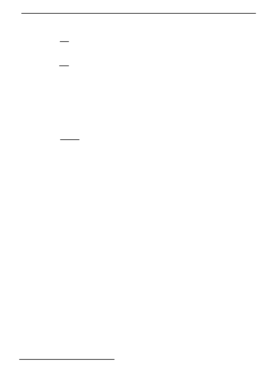
For our purposes, a control system is an equation of the type (1.1), with input u and state
x. Once the input u and the intial state x(t
i
) = x
i
are specified, the state x is determined. So
one can think of a control system as a box, which given the input u and intial state x(t
i
) = x
i
,
manufactures the state according to the law (1.1); see Figure 1.1.
If the function f is linear, that is, if f (
x, u) = Ax + Bu for some A ∈ R
n×n
and B
∈ R
n×m
,
then the control system is said to be linear.
Exercises.
1
By a
R
m
-valued piecewise continuous function on an interval [
a, b], we mean a function f : [a, b] → R
m
such that there exist finitely many points
t
1
, . . . , t
k
∈ [a, b] such that f is continuous on each of the intervals
(
a, t
1
)
, (t
1
, t
2
)
, . . . , (t
k−1
, t
k
)
, (t
k
, b), the left- and right- hand limits lim
tt
l
f(t) and lim
tt
l
f(t) exist for all l ∈
{1, . . . , k}, and lim
ta
f(t) and lim
tt
b
f(t) exist.
1.3. Questions in control theory
3
plant
˙
x(t) = f (x(t), u(t))
x(t
i
) = x
i
u
x
Figure 1.1: A control system.
1. (Linear control system.)
Let A
∈ R
n
and B
∈ R
n×m
. Prove that if u is a continuous
function, then the differential equation
dx
dt
(t) = Ax(t) + Bu(t), x(t
i
) = x
i
, t
≥ t
i
(1.3)
has a unique solution x(
·) in [t
i
, +
∞) given by
x(t) = e
(t−t
i
)A
x
i
+ e
tA
t
t
i
e
−τA
Bu(τ )dτ.
2. Consider the scalar Riccati equation
˙
p(t) = γ(p(t) + α)(p(t) + β).
Prove that
q(t) :=
1
p(t) + α
satisfies the following differential equation
˙
q(t) = γ(α
− β)q(t) − γ.
3. Solve
˙
p(t) = (p(t))
2
− 1, t ∈ [0, 1], p(1) = 0.
A characteristic of underdetermined equations is that one can choose the free variable in a
way that some desirable effect is produced on the other dependent variable. For example, if with
our algebraic equation x + u = 10 we wish to make x < 5, then we can achieve this by choosing
the free variable u to be strictly larger than 5. Control theory is all about doing similar things
with differential equations of the type (1.1). The state variables x comprise the ‘to-be-controlled’
variables, which depend on the free variables u, the inputs. For example, in the case of an aircraft,
the speed, altitude and so on are the to-be-controlled variables, while the angle of the wing flaps,
the speed of the propeller and so on, which the pilot can specify, are the inputs.
1.3
Questions in control theory
1. How do we choose the control inputs to achieve regulation of the state variables?
For instance, we might want the state x to track some desired reference state x
r
, and there
must be stability under external disturbances. For example, a thermostat is a device in
an air conditioner that changes the input in such a way that the temperature tracks a
constant reference temperature and there is stability despite external disturbances (doors
being opened or closed, change in the number of people in the room, activity in the kitchen
etcetera): if the temperature in the room goes above the reference value, then the thermostat

4
Chapter 1. Introduction
(which is a bimetallic strip) bends and closes the circuit so that electricity flows and the air
conditioner produces a cooling action; on the other hand if the temperature in the room
drops below the reference value, the bimetallic strip bends the other way hence breaking the
circuit and the air conditioner produces no further cooling. These problems of regulation
are mostly the domain of control theory for engineering systems. In economic systems, one
is furthermore interested in extreme performances of control systems. This naturally brings
us to the other important question in control theory, which is the realm of optimal control
theory.
2. How do we control optimally?
Tools from calculus of variations are employed here. These questions of optimality arise
naturally. For example, in the case of an aircraft, we are not just interested in flying from
one place to another, but we would also like to do so in a way so that the total travel time
is minimized or the fuel consumption is minimized. With our algebraic equation x + u = 10,
in which we want x < 5, suppose that furthermore we wish to do so in manner such that
u is the least possible integer. Then the only possible choice of the (input) u is 6. Optimal
control addresses similar questions with differential equations of the type (1.1), together with
a ‘performance index functional’, which is a function that measures optimality.
This course is about the basic principles behind optimal control theory.
1.4
Appendix: systems of differential equations and
e
tA
In this appendix, we introduce the exponential of a matrix, which is useful for obtaining explicit
solutions to the linear control system (1.3) in the exercise 1 on page 3. We begin with a few
preliminaries concerning vector-valued functions.
With a slight abuse of notation, a vector-valued function x(t) is a vector whose entries are
functions of t. Similarly, a matrix-valued function A(t) is a matrix whose entries are functions:
⎡
⎢
⎣
x
1
(t)
..
.
x
n
(t)
⎤
⎥
⎦ , A(t) =
⎡
⎢
⎣
a
11
(t)
. . .
a
1n
(t)
..
.
..
.
a
m1
(t)
. . .
a
mn
(t)
⎤
⎥
⎦ .
The calculus operations of taking limits, differentiating, and so on are extended to vector-valued
and matrix-valued functions by performing the operations on each entry separately. Thus by
definition,
lim
t→t
0
x(t) =
⎡
⎢
⎣
lim
t→t
0
x
1
(t)
..
.
lim
t→t
0
x
n
(t)
⎤
⎥
⎦ .
So this limit exists iff lim
t→t
0
x
i
(t) exists for all i
∈ {1, . . . , n}. Similiarly, the derivative of
a vector-valued or matrix-valued function is the function obtained by differentiating each entry
separately:
dx
dt
(t) =
⎡
⎢
⎣
x
1
(t)
..
.
x
n
(t)
⎤
⎥
⎦ ,
dA
dt
(t) =
⎡
⎢
⎣
a
11
(t)
. . .
a
1n
(t)
..
.
..
.
a
m1
(t)
. . .
a
mn
(t)
⎤
⎥
⎦ ,
where x
i
(t) is the derivative of x
i
(t), and so on. So
dx
dt
is defined iff each of the functions x
i
(t) is
differentiable. The derivative can also be described in vector notation, as
dx
dt
(t) = lim
h→0
x(t + h)
− x(t)
h
.
(1.4)

1.4. Appendix: systems of differential equations and
e
tA
5
Here x(t + h)
− x(t) is computed by vector addition and the h in the denominator stands for
scalr multiplication by h
−1
. The limit is obtained by evaluating the limit of each entry separately,
as above. So the entries of (1.4) are the derivatives x
i
(t). The same is true for matrix-valued
functions.
A system of homogeneous, first-order, linear constant-coefficient differential equations is a
matrix equation of the form
dx
dt
(t) = Ax(t),
(1.5)
where A is a n
× n real matrix and x(t) is an n dimensional vector-valued function. Writing out
such a system, we obtain a system of n differential equations, of the form
dx
1
dt
(t)
=
a
11
x
1
(t) +
· · · + a
1n
x
n
(t)
. . .
dx
n
dt
(t)
=
a
n1
x
1
(t) +
· · · + a
nn
x
n
(t).
The x
i
(t) are unknown functions, and the a
ij
are scalars. For example, if we substitute the matrix
3
−2
1
4
for A, (1.5) becomes a system of two equations in two unknowns:
dx
1
dt
(t)
=
3x
1
(t)
− 2x
2
(t)
dx
2
dt
(t)
=
x
1
(t) + 4x
2
(t).
Now consider the case when the matrix A is simply a scalar. We learn in calculus that the
solutions to the first-order scalar linear differential equation
dx
dt
(t) = ax(t)
are x(t) = ce
ta
, c being an arbitrary constant. Indeed, ce
ta
obviously solves this equation. To
show that every solution has this form, let x(t) be an arbitrary differentiable function which is a
solution. We differentiate e
−ta
x(t) using the product rule:
d
dt
(e
−ta
x(t)) =
−ae
−ta
x(t) + e
−ta
ax(t) = 0.
Thus e
−ta
x(t) is a constant, say c, and x(t) = ce
ta
. Now suppose that analogous to
e
a
= 1 + a +
a
2
2!
+
a
3
3!
+ . . . , a
∈ R,
we define
e
A
= I + A +
1
2!
A
2
+
1
3!
A
3
+ . . . , A
∈ R
n×n
.
(1.6)
Later in this section, we study this matrix exponential, and use the matrix-valued function
e
tA
= I + tA +
t
2
2!
A
2
+
t
3
3!
A
2
+ . . .
(where t is a variable scalar) to solve (1.5). We begin by stating the following result, which shows
that the series in (1.6) converges for any given square matrix A.
6
Chapter 1. Introduction
Theorem 1.4.1
The series (1.6) converges for any given square matrix A.
We have collected the proofs together at the end of this section in order to not break up the
discussion.
Since matrix multiplication is relatively complicated, it isn’t easy to write down the matrix
entries of e
A
directly. In particular, the entries of e
A
are usually not obtained by exponentiating
the entries of A. However, one case in which the exponential is easily computed, is when A is
a diagonal matrix, say with diagonal entries λ
i
. Inspection of the series shows that e
A
is also
diagonal in this case and that its diagonal entries are e
λ
i
.
The exponential of a matrix A can also be determined when A is diagonalizable , that is,
whenever we know a matrix P such that P
−1
AP is a diagonal matrix D. Then A = P DP
−1
, and
using (P DP
−1
)
k
= P D
k
P
−1
, we obtain
e
A
=
I + A +
1
2!
A
2
+
1
3!
A
3
+ . . .
=
I + P DP
−1
+
1
2!
2
P D
2
P
−1
+
1
3!
P D
3
P
−1
+ . . .
=
P IP
−
+ P DP
−1
+
1
2!
2
P D
2
P
−1
+
1
3!
P D
3
P
−1
+ . . .
=
P
I + D +
1
2!
D
2
+
1
3!
D
3
+ . . .
P
−1
=
P e
D
P
−1
=
P
⎡
⎢
⎣
e
λ
1
0
. ..
e
λ
n
⎤
⎥
⎦ P
−1
,
where λ
1
, . . . , λ
n
denote the eigenvalues of A.
Exercise. (
∗) The set of diagonalizable n × n real matrices is dense in the set of all n × n real
matrices, that is, given any A
∈ R
n×n
, there exists a B
∈ R
n×n
arbitrarily close to A (meaning
that
|b
ij
− a
ij
| can be made arbitrarily small for all i, j ∈ {1, . . . , n}) such that B has n distinct
eigenvalues.
In order to use the matrix exponential to solve systems of differential equations, we need to
extend some of the properties of the ordinary exponential to it. The most fundamental property
is e
a+b
= e
a
e
b
. This property can be expressed as a formal identity between the two infinite series
which are obtained by expanding
e
a+b
= 1 +
(a+b)
1!
+
(a+b)
2
2!
+ . . . and
e
a
e
b
=
1 +
a
1!
+
a
2
2!
+ . . .
1 +
b
1!
+
b
2
2!
+ . . .
.
(1.7)
We cannot substitute matrices into this identity because the commutative law is needed to obtain
equality of the two series. For instance, the quadratic terms of (1.7), computed without the
commutative law, are
1
2
(a
2
+ ab + ba + b
2
) and
1
2
a
2
+ ab +
1
2
b
2
. They are not equal unless ab = ba.
So there is no reason to expect e
A+B
to equal e
A
e
B
in general. However, if two matrices A and
B happen to commute, the formal identity can be applied.
Theorem 1.4.2
If A, B
∈ R
n×n
commute (that is AB = BA), then e
A+B
= e
A
e
B
.

1.4. Appendix: systems of differential equations and
e
tA
7
The proof is at the end of this section. Note that the above implies that e
A
is always invertible
and in fact its inverse is e
−A
: Indeed I = e
A−A
= e
A
e
−A
.
Exercises.
1. Give an example of 2
× 2 matrices A and B such that e
A+B
= e
A
e
B
.
2. Compute e
A
, where A is given by
A =
2
3
0
2
.
Hint: A = 2I +
0
3
0
0
.
We now come to the main result relating the matrix exponential to differential equations.
Given an n
× n matrix, we consider the exponential e
tA
, t being a variable scalar, as a matrix-
valued function:
e
tA
= I + tA +
t
2
2!
A
2
+
t
3
3!
A
3
+ . . . .
Theorem 1.4.3
e
tA
is a differentiable matrix-valued function of t, and its derivative is e
tA
.
The proof is at the end of the section.
Theorem 1.4.4 (Product rule.)
Let A(t) and B(t) be differentiable matrix-valued functions of t,
of suitable sizes so that their product is defined. Then the matrix product A(t)B(t) is differentiable,
and its derivative is
d
dt
(A(t)B(t)) =
dA(t)
dt
B(t) + A(t)
dB(t)
dt
.
The proof is left as an exercise.
Theorem 1.4.5
The first-order linear differential equation
dx
dt
(t) = Ax(t), t
≥ t
i
, x(t
i
) = x
i
has the unique solution x(t) = e
(t−t
i
)A
x
i
.
Proof

Chapter 2
The optimal control problem
2.1
Introduction
Optimal control theory is about controlling the given system in some ‘best’ way. The optimal
control strategy will depend on what is defined as the best way. This is usually specified in terms
of a performance index functional.
As a simple example, consider the problem of a rocket launching a satellite into an orbit about
the earth. An associated optimal control problem is to choose the controls (the thrust attitude
angle and the rate of emission of the exhaust gases) so that the rocket takes the satellite into its
prescribed orbit with minimum expenditure of fuel or in minimum time.
We first look at a number of specific examples that motivate the general form for optimal
control problems, and having seen these, we give the statement of the optimal control problem
that we study in these notes in
§2.4.
2.2
Examples of optimal control problems
Example.
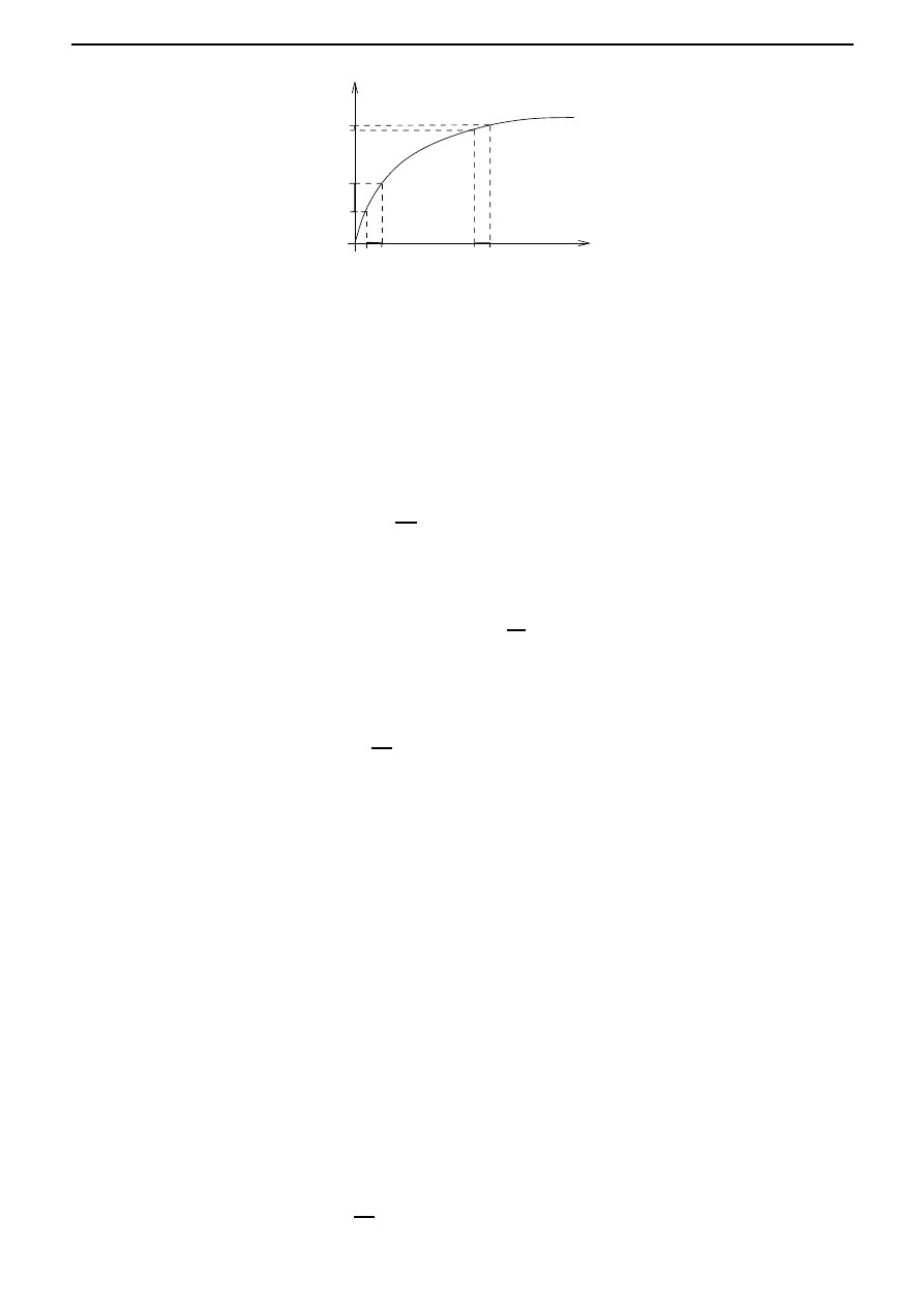
(Economic growth.) We first consider a mathematical model of a simplified economy
in which the rate of output Y is assumed to depend on the rates of input of capital K (for example
in the form of machinery) and labour force L, that is,
Y = P (K, L)
where P is called the production function. This function is assumed to have the following ‘scaling’
property
P (αK, αL) = αP (K, L).
With α =
1
L
, and defining the output rate per worker as y =
Y
L
and the capital rate per worker
as k =
K
L
, we have
y =
Y
L
=
1
L
P (K, L) = P
K
L
,
L
L
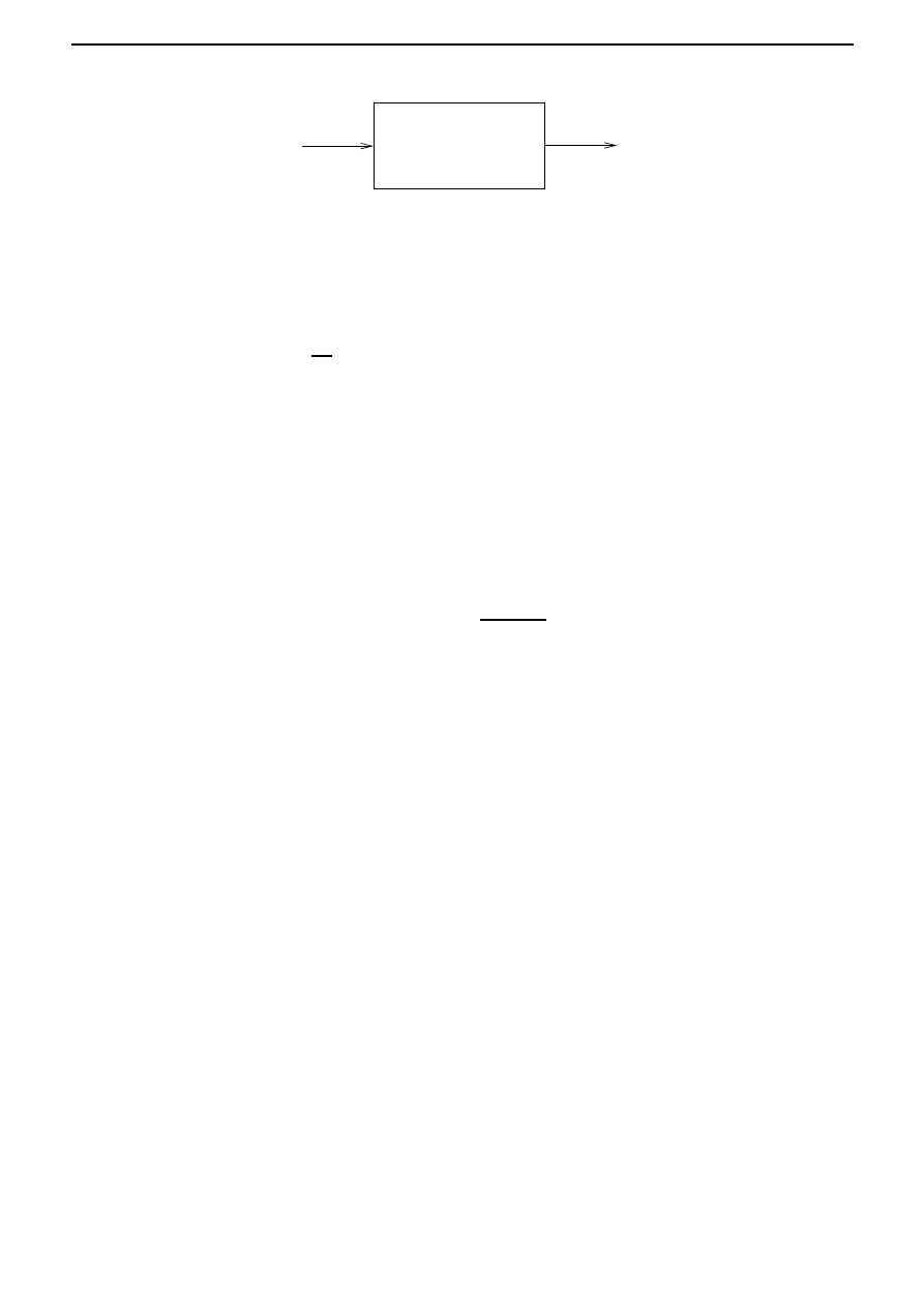
= P (k, 1) = Π(k), say.
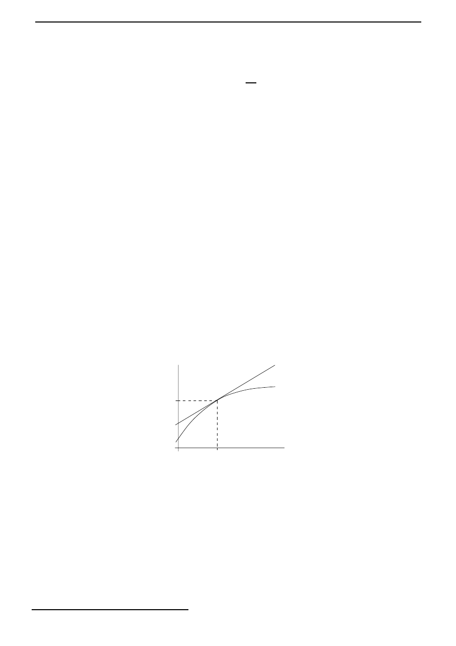
A typical form of Π is illustrated in Figure 2.1; we note that Π(
k) > 0, but Π
(
k) < 0. Output is
either consumed or invested, so that
Y = C + I,
9
10
Chapter 2. The optimal control problem
Π
k
Figure 2.1: Production function Π.
where C and I are the rates of consumption and investment, respectively.
The investment is used to increase the capital stock and replace machinery, that is
I(t) =
dK
dt
(t) + μK(t),
where μ is called the rate of depreciation. Defining c =
C
L
as the consumption rate per worker, we
obtain
y(t) = Π(k(t)) = c(t) +
1
L(t)
dK
dt
(t) + μk(t).
Since
d
dt
K
L
=
1
L
dK
dt
−
k
L
dL
dt
,
it follows that
Π(k) = c +
dk
dt
+
˙
L
L
k + μk.
Assuming that labour grows exponentially, that is L(t) = L
0
e
λt
, we have
dk
dt
(t) = Π(k(t))
− (λ + μ)k(t) − c(t),
which is the governing equation of this economic growth model. The consumption rate per worker,
namely c, is the control input for this problem.
The central planner’s problem is to choose c on a time interval [0, T ] in some best way. But
what are the desired economic objectives that define this best way? One method of quantifying
the best way is to introduce a ‘utility’ function U ; which is a measure of the value attached
to the consumption. The function U normally satisfies U
(
c) ≤ 0, which means that a fixed
increment in consumption will be valued increasingly highly with decreasing consumption level.
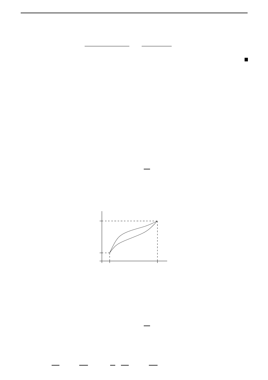
This is illustrated in Figure 2.2. We also need to optimize consumption for [0, T ], but with some
discounting for future time. So the central planner wishes to maximize the ‘welfare’ integral
W (c) =
T
0
e
−δt
U (c(t))dt,
where δ is known as the discount rate, which is a measure of preference for earlier rather than
later consumption. If δ = 0, then there is no time discounting and consumption is valued equally
at all times; as δ increases, so does the discounting of consumption and utility at future times.
The mathematical problem has now been reduced to finding the optimal consumption path
{c(t), t ∈ [0, T ]}, which maximizes W subject to the constraint
dk
dt
(t) = Π(k(t))
− (λ + μ)k(t) − c(t),
2.2. Examples of optimal control problems
11
U
c
Figure 2.2: Utility function U .
and with k(0) = k
0
.
Example.
(Exploited populations.) Many resources are to some extent renewable (for example,
fish populations, grazing land, forests) and a vital problem is their optimal management. With
no harvesting, the resource population x is assumed to obey a growth law of the form
dx
dt
(t) = ρ(x(t)).
(2.1)
A typical example for ρ is the Verhulst model
ρ(
x) = ρ
0
x
1
−
x
x
s
,
where
x
s
is the saturation level of population, and ρ
0
is a positive constant. With harvesting,
(2.1) is modified to
dx
dt
(t) = ρ(x(t))
− h(t)
where h is the harvesting rate. Now h will depend on the fishing effort e (for example, size of nets,
number of trawlers, number of fishing days) as well as the population level, so that we assume
h(t) = e(t)x(t).
Optimal management will seek to maximize the economic rent defined by
r(t) = ph(t)
− ce(t),
assuming the cost to be proportional to the effort, and where p is the unit price.
The problem is to maximize the discounted economic rent, called the present value V , over
some period [0, T ], that is,
V (e) =
T
0
e
−δt
(pe(t)x(t)
− ce(t))dt,
subject to
dx
dt
(t) = ρ(x(t))
− e(t)x(t),
and the initial condition x(0) = x
0
.

12
Chapter 2. The optimal control problem
2.3
Functionals
The examples from the previous section involve finding extremum values of integrals subject to a
differential equation constraint. These integrals are particular examples of a ‘functional’.
A functional is a correspondence which assigns a definite real number to each function be-
longing to some class. Thus, one might say that a functional is a kind of function, where the
independent variable is itself a function.
Examples. The following are examples of functionals:
1. Consider the set of all rectifiable plane curves
1
. A definite number associated with each such
curve, is for instance, its length. Thus the length of a curve is a functional defined on the
set of rectifiable curves.
2. Let x be an arbitrary continuously differentiable function defined on [t
i
, t
f
]. Then the formula
I(x) =
t
f
t
i
dx
dt
(t)
2
dt
defines a functional on the set of all such functions x.
3. As a more general example, let F (
x, x
,
t) be a continuous function of three variables. Then
the expression
I(x) =
t
f
t
i
F
x(t),
dx
dt
(t), t
dt,
where x ranges over the set of all continuously differentiable functions defined on the interval
[t
i
, t
f
], defines a functional.
By choosing different functions F , we obtain different functionals. For example, if
F (
x, x
,
t) =
1 + (
x
)
2
,
then I(x) is the length of the curve
{x(t), t ∈ [t
i
, t
f
]
}, as in the first example, while if
F (
x, x
,
t) = (x
)
2
,
then I(x) reduces to the case considered in the second example.
4. Let f (
x, u) and F (x, u, t) be continuously differentiable functions of their arguments. Given
a continuous function u on [t
i
, t
f
], let x denote the unique solution of
dx
dt
(t) = f (x(t), u(t)), x(t
i
) = x
i
, t
∈ [t
i
, t
f
].
Then I given by
I
x
i
(u) =
t
f
t
i
F (x(t), u(t), t)dt
defines a functional on the set of all continuous functions u on [t
i
, t
f
].
1
In analysis, the length of a curve is defined as the limiting length of a polygonal line inscribed in the curve
(that is, with vertices lying on the curve) as the maximum length of the chords forming the polygonal line goes to
zero. If this limit exists and is finite, then the curve is said to be rectifiable.

2.4. The general form of the basic optimal control problem
13
Exercise.
(A path-independent functional.) Consider the set of all continuously differentiable
functions x defined on [t
i
, t
f
] such that x(t
i
) = x
i
and x(t
f
) = x
f
, and let
I(x) =
t
f
t
i
x(t) + t
dx
dt
(t)
dt.
Show that I is independent of path. What is its value?
Remark. Such a functional is analogous to the notion of a constant function
f :
R → R, for
which the problem of finding extremal points is trivial: indeed since the value is constant, every
point serves as a point which maximizes/minimizes the functional.
2.4
The general form of the basic optimal control problem
The examples discussed in
§2.2 can be put in the following form. As mentioned in the introduction,
we assume that the state of the system satisfies the coupled first order differential equations
dx
1
dt
(t)
=
f
1
(x
1
(t), . . . , x
n
(t), u
1
(t), . . . , u
m
(t)), x
1
(t
0
) = x
i,1
..
.
dx
n
dt
(t)
=
f
n
(x
1
(t), . . . , x
n
(t), u
1
(t), . . . , u
m
(t)), x
n
(t
0
) = x
i,n
,
on [t
i
, t
f
], and where the m variables u
1
, . . . , u
m
form the control input vector u. We can conve-
niently write the system of equations above in the form
dx
dt
(t) = f (x(t), u(t)), x(t
i
) = x
i
, t
∈ [t
i
, t
f
].
We assume that u
∈ (C[t
i
, t
f
])
m
, that is, each component of u is a continuous function on [t
i
, t
f
].
It is also assumed that f
1
, . . . , f
n
possess partial derivatives with respect to
x
k
, 1
≤ k ≤ n and
u
l
, 1
≤ l ≤ m and these are continuous. (So f is continuously differentiable in both variables.)
The initial value of x is specified (x
i
at time t
i
), which means that specifying u(t) for t
∈ [t
i
, t
f
]
determines x (see Theorem 1.2.1).
The basic optimal control problem is to choose the control u
∈ (C[t
i
, t
f
])
m
such that:
1. The state x is transferred from x
i
to a state at terminal time t
f
where some (or all or none)
of the state variable components are specified; for example, without loss of generality
2
x(t
f
)
k
is specified for k
∈ {1, . . . , r}.
2. The functional
I
x
i
(u) =
t
f
t
i
F (x(t), u(t), t)dt
is minimized
3
.
A function u
∗
that minimizes the functional I is called an optimal control, the corresponding state
x
∗
is called the optimal state, and the pair (x
∗
, u
∗
) is called an optimal trajectory. Using the
notation above, we can identify the two optimal control problem examples listed in
§2.2.
2
Or else, we may shuffle the components of
x.
3
Note that a maximization problem for
I
x
i
can be converted into a minimization problem by considering the
functional
−I
x
i
instead of
I
x
i
.

14
Chapter 2. The optimal control problem
Example.
(Economic growth, continued.) We have
n
=
1,
m
=
1,
x
=
k,
u
=
c,
f (
x, u) = Π(x) − (λ + μ)x − u,
F (
x, u, t) = e
−δt
U (
u).

Chapter 3
Calculus of variations
3.1
Introduction
Before we attempt solving the optimal control problem described in Section 2.4 of Chapter 2,
that is, an extremum problem for a functional of the type described in item 4 on page 12, we
consider the following simpler problem in this chapter: we would like to find extremal curves x for
a functional of the type described in item 3 on page 12. This is simpler since there is no differential
equation constraint.
In order to solve this problem, we first make the problem more abstract by considering the
problem of finding extremal points x
∗
∈ X for a functional I : X → R, where X is a normed linear
space. (The notion of a normed linear space is introduced in Section 3.4.) We develop a calculus
for solving such problems. This situation is entirely analogous to the problem of finding extremal
points for a differentiable function f :
R → R:
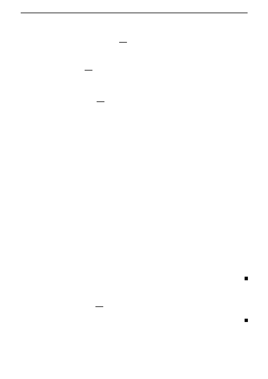
Consider for example the quadratic function f (x) = ax
2
+ bx + c. Suppose that one wants
to know the points x
∗
at which f assumes a maximum or a minimum. We know that if f has
a maximum or a minimum at the point x
∗
, then the derivative of the function must be zero at
that point: f
(x
∗
) = 0. See Figure 3.1. So one can then one can proceed as follows. First find
the expression for the derivative: f
(x) = 2ax + b. Next solve for the unknown x
∗
in the equation
f
(x
∗
) = 0, that is,
2ax
∗
+ b = 0
(3.1)
and so we find that a candidate for the point x
∗
which minimizes or maximizes f is x
∗
=
−
b
2a
,
which is obtained by solving the algebraic equation (3.1) above.
x
x
x
∗
x
∗
f
f
Figure 3.1: Necessary condition for x
∗
to be an extremal point for f is that f
(x
∗
) = 0.
We wish to do the above with functionals. In order to do this we need a notion of derivative of
a functional, and an analogue of the fact above concerning the necessity of the vanishing derivative
15
16
Chapter 3. Calculus of variations
at extremal points. We define the derivative of a functional I : X
→ R in Section 3.4, and also
prove Theorem 3.4.2, which says that this derivative must vanish at an extremal point x
∗
∈ X.
In the remainder of the chapter, we apply Theorem 3.4.2 to the concrete case where X com-
prises continuously differentiable functions, and I is a functional of the form
I(x) =
t
f
t
i
F (x(t), x
(t), t)dt.
(3.2)
We find the derivative of such a functional, and equating it to zero, we obtain a necessary condi-
tion that an extremal curve should satisfy: instead of an algebraic equation (3.1), we now obtain
a differential equation, called the Euler-Lagrange equation, given by (3.9). Continuously differen-
tiable solutions x
∗
of this differential equation are then candidates which maximize or minimize
the functional I. Historically speaking, such optimization problems arising from physics gave birth
to the subject of ‘calculus of variations’. We begin this chapter with the discussion of one such
milestone problem, called the ‘brachistochrone problem’ (brachistos=shortest, chronos=time).
3.2
The brachistochrone problem
The calculus of variations originated from a problem posed by the Swiss mathematician Johann
Bernoulli (1667-1748). He required the form of the curve joining two fixed points A and B in a
vertical plane such that a body sliding down the curve (under gravity and no friction) travels from
A to B in minimum time. This problem does not have a trivial solution; the straight line from A
to B is not the solution (this is also intuitively clear, since if the slope is high at the beginning,
the body picks up a high velocity and so its plausible that the travel time could be reduced) and
it can be verified experimentally by sliding beads down wires in appropriate shapes.
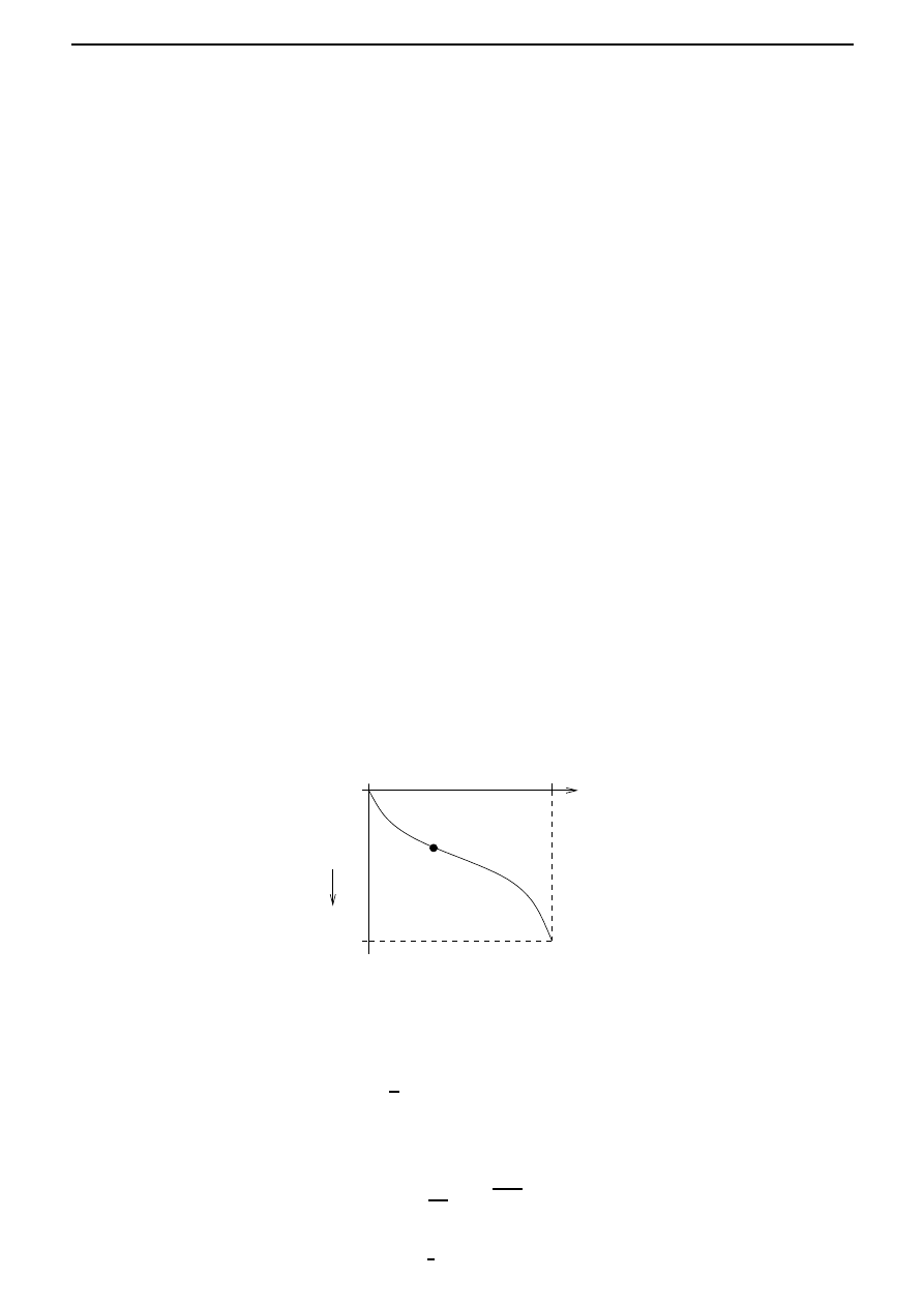
To pose the problem in mathematical terms, we introduce coordinates as shown in Figure 3.2,
so that A is the point (0, 0), and B corresponds to (x
0
, y
0
). Assuming that the particle is released
A (0, 0)
B (x
0
, y
0
)
gravity
y
0
x
0
x
y
Figure 3.2: The brachistochrone problem.
from rest at A, conservation of energy gives
1
2
mv
2
− mgy = 0,
(3.3)
where we have taken the zero potential energy level at y = 0, and where v denotes the speed of
the particle. Thus the speed is given by
v =
ds
dt
=
2gy,
(3.4)
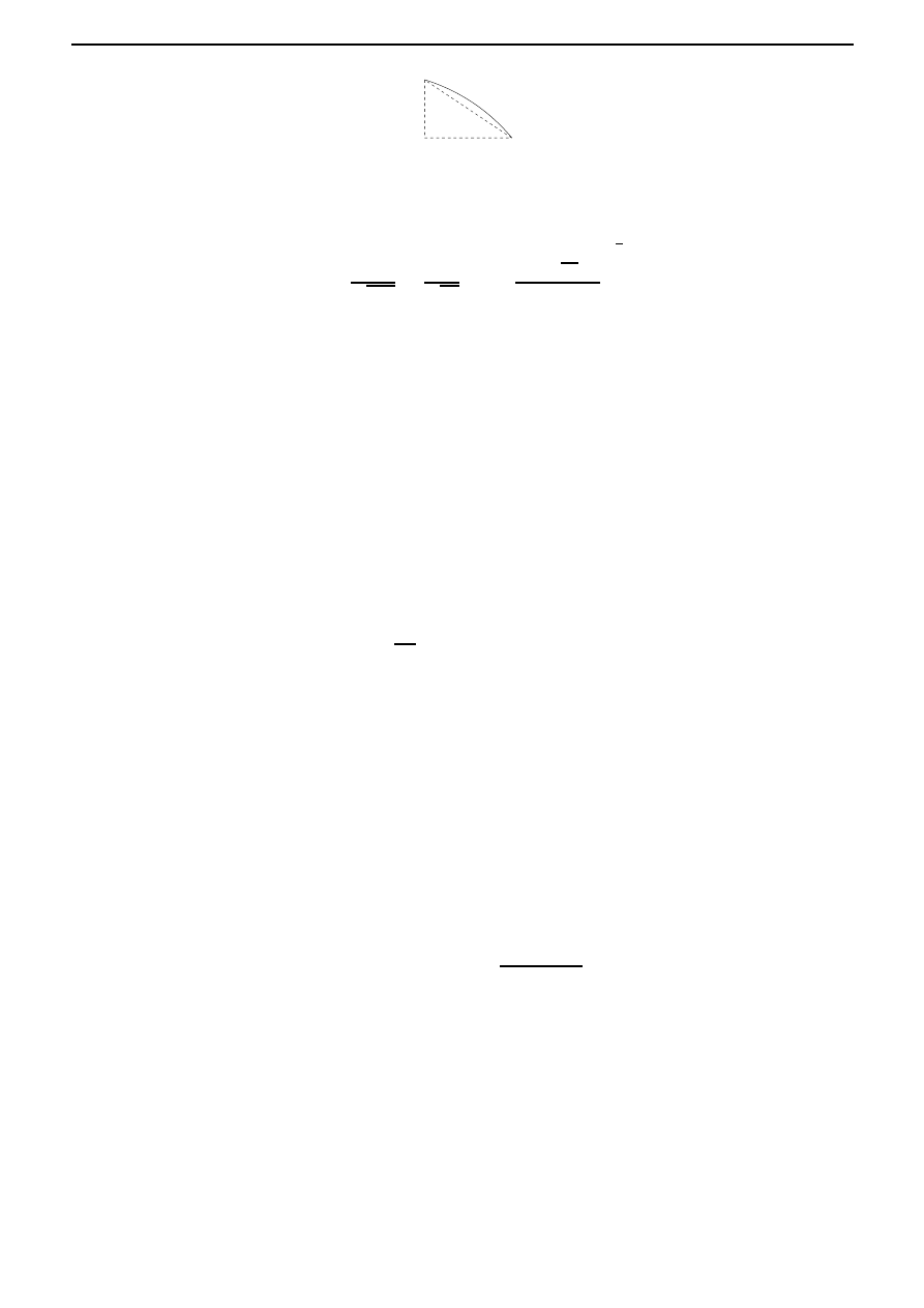
where s denotes arc length along the curve. From Figure 3.3, we see that an element of arc length,
δs is given approximately by ((δx)
2
+ (δy)
2
)
1
2
. Hence the time of descent is given by
3.3. Calculus of variations versus extremum problems of functions of
n real variables
17
δy
δx
δs
Figure 3.3: Element of arc length.
T =
curve
ds
√
2gy
=
1
√
2g
y
0
0
⎡
⎢
⎣
1 +
dx
dy
2
y
⎤
⎥
⎦
1
2
dy.
Our problem is to find the path
{x(y), y ∈ [0, y
0
]
}, satisfying x(0) = 0 and x(y
0
) = x
0
, which
minimizes T .
3.3
Calculus of variations versus extremum problems of
functions of
n real variables
To understand the basic meaning of the problems and methods of the calculus of variations, it is
important to see how they are related to the problems of the study of functions of n real variables.
Thus, consider a functional of the form
I(x) =
t
f
t
i
F
x(t),
dx
dt
(t), t
dt, x(t
i
) = x
i
, x(t
f
) = x
f
.
Here each curve x is assigned a certain number. To find a related function of the sort considered
in classical analysis, we may proceed as follows. Using the points
t
i
= t
0
, t
1
, . . . , t
n
, t
n+1
= t
f
,
we divide the interval [t
i
, t
f
] into n + 1 equal parts. Then we replace the curve
{x(t), t ∈ [t
i
, t
f
]
}
by the polygonal line joining the points
(t
0
, x
i
), (t
1
, x(t
1
)), . . . , (t
n
, x(t
n
)), (t
n+1
, x
f
),
and we approximate the functional I at x by the sum
I
n
(x
1
, . . . , x
n
) =
n
k=1
F
x
k
,
x
k
− x
k−1
h
k
, t
k
h
k
,
(3.5)
where x
k
= x(t
k
) and h
k
= t
k
− t
k−1
. Each polygonal line is uniquely determined by the ordinates
x
1
, . . . , x
n
of its vertices (recall that x
0
= x
i
and x
n+1
= x
f
are fixed), and the sum (3.5) is
therefore a function of the n variables x
1
, . . . , x
n
. Thus as an approximation, we can regard the
variational problem as the problem of finding the extrema of the function I
n
(x
1
, . . . , x
n
).
In solving variational problems, Euler made extensive use of this ‘method of finite differences’.
By replacing smooth curves by polygonal lines, he reduced the problem of finding extrema of a
functional to the problem of finding extrema of a function of n variables, and then he obtained
exact solutions by passing to the limit as n
→ ∞. In this sense, functionals can be regarded
as ‘functions of infinitely many variables’ (that is, the infinitely many values of x(t) at different
points), and the calculus of variations can be regarded as the corresponding analog of differential
calculus of functions of n real variables.

18
Chapter 3. Calculus of variations
3.4
Calculus in function spaces and beyond
In the study of functions of a finite number of n variables, it is convenient to use geometric
language, by regarding a set of n numbers (x
1
, . . . , x
n
) as a point in an n-dimensional space. In
the same way, geometric language is useful when studying functionals. Thus, we regard each
function x(
·) belonging to some class as a point in some space, and spaces whose elements are
functions will be called function spaces.
In the study of functions of a finite number n of independent variables, it is sufficient to consider
a single space, that is, n-dimensional Euclidean space
R
n
. However, in the case of function spaces,
there is no such ‘universal’ space. In fact, the nature of the problem under consideration determines
the choice of the function space. For instance, if we consider a functional of the form
I(x) =
t
f
t
i
F
x(t),
dx
dt
(t), t
dt,
then it is natural to regard the functional as defined on the set of all functions with a continuous
first derivative.
The concept of continuity plays an important role for functionals, just as it does for the ordi-
nary functions considered in classical analysis. In order to formulate this concept for functionals,
we must somehow introduce a notion of ‘closeness’ for elements in a function space. This is most
conveniently done by introducing the concept of the norm of a function, analogous to the concept
of the distance between a point in Euclidean space and the origin. Although in what follows we
shall always be concerned with function spaces, it will be most convenient to introduce the concept
of a norm in a more general and abstract form, by introducing the concept of a normed linear
space.
By a linear space (or vector space) over
R, we mean a set X together with the operations of
addition + : X
× X → X and scalar multiplication · : R × X → X that satisfy the following:
1. x
1
+ (x
2
+ x
3
) = (x
1
+ x
2
) + x
3
for all x
1
, x
2
, x
3
∈ X.
2. There exists an element, denoted by 0 (called the zero element) such that x + 0 = 0 + x = x
for all x
∈ X.
3. For every x
∈ X, there exists an element, denoted by −x such that x+(−x) = (−x)+x = 0.
4. x
1
+ x
2
= x
2
+ x
1
for all x
1
, x
2
∈ X.
5. 1
· x = x for all x ∈ X.
6. α
· (β · x) = (αβ) · x for all α, β ∈ R and for all x ∈ X.
7. (α + β)
· x = α · x + β · x for all α, β ∈ R and for all x ∈ X.
8. α
· (x
1
+ x
2
) = α
· x
1
+ α
· x
2
for all α
∈ R and for all x
1
, x
2
∈ X.
A linear functional L : X
→ R is a map that satisfies
1. L(x
1
+ x
2
) = L(x
1
) + L(x
2
) for all x
1
, x
2
∈ X.
2. L(α
· x) = αL(x) for all α ∈ R and for all x ∈ X.

3.4. Calculus in function spaces and beyond
19
The set ker(L) =
{x ∈ X | L(x) = 0} is called the kernel of the linear functional L.
Exercise. (
∗) If L
1
, L
2
are linear functionals defined on X such that ker(L
1
)
⊂ ker(L
2
), then
prove that there exists a constant λ
∈ R such that L
2
(x) = λL
1
(x) for all x
∈ X.
Hint: The case when L
1
= 0 is trivial. For the other case, first prove that if ker(L
1
)
= X, then
there exists a x
0
∈ X such that X = ker(L
1
) + [x
0
], where [x
0
] denotes the linear span of x
0
.
What is L
2
x for x
∈ X?
A linear space over
R is said to be normed, if there exists a function · : X → [0, ∞) (called
norm), such that:
1.
x = 0 iff x = 0.
2.
α · x = |α| x for all α ∈ R and for all x ∈ X.
3.
x
1
+ x
2
≤ x
1
+ x
2
for all x
1
, x
2
∈ X. (Triangle inequality.)
In a normed linear space, we can talk about distances between elements, by defining the distance
between x
1
and x
2
to be the quantity
x
1
− x
2
. In this manner, a normed linear space becomes
a metric space. Recall that a metric space is a set X together with a function d : X
× X → R,
called distance, that satisfies
1. d(x, y)
≥ 0 for all x, y in X, and d(x, y) = 0 iff x = y.
2. d(x, y) = d(y, x) for all x, y in X.
3. d(x, z)
≤ d(x, y) + d(y, z) for all x, y, z in X.
Exercise. Let (
X,
· ) be a normed linear space. Prove that (X, d) is a metric space, where
d : X
× X → [0, ∞) is defined by d(x
1
, x
2
) =
x
1
− x
2
, x
1
, x
2
∈ X.
The elements of a normed linear space can be objects of any kind, for example, numbers,
matrices, functions, etcetera. The following normed spaces are important for our subsequent
purposes:
1. C[t
i
, t
f
].
The space C[t
i
, t
f
] consists of all continuous functions x(
·) defined on the closed interval
[t
i
, t
f
]. By addition of elements of C[t
i
, t
f
], we mean pointwise addition of functions: for
x
1
, x
2
∈ C[t
i
, t
f
], (x
1
+ x
2
)(t) = x
1
(t) + x
2
(t) for all t
∈ [t
i
, t
f
]. Scalar multiplication is
defined as follows: (α
· x)(t) = αx(t) for all t ∈ [t
i
, t
f
]. The norm is defined as the maximum
of the absolute value:
x = max
t∈[t
i
,t
f
]
|x(t)|.
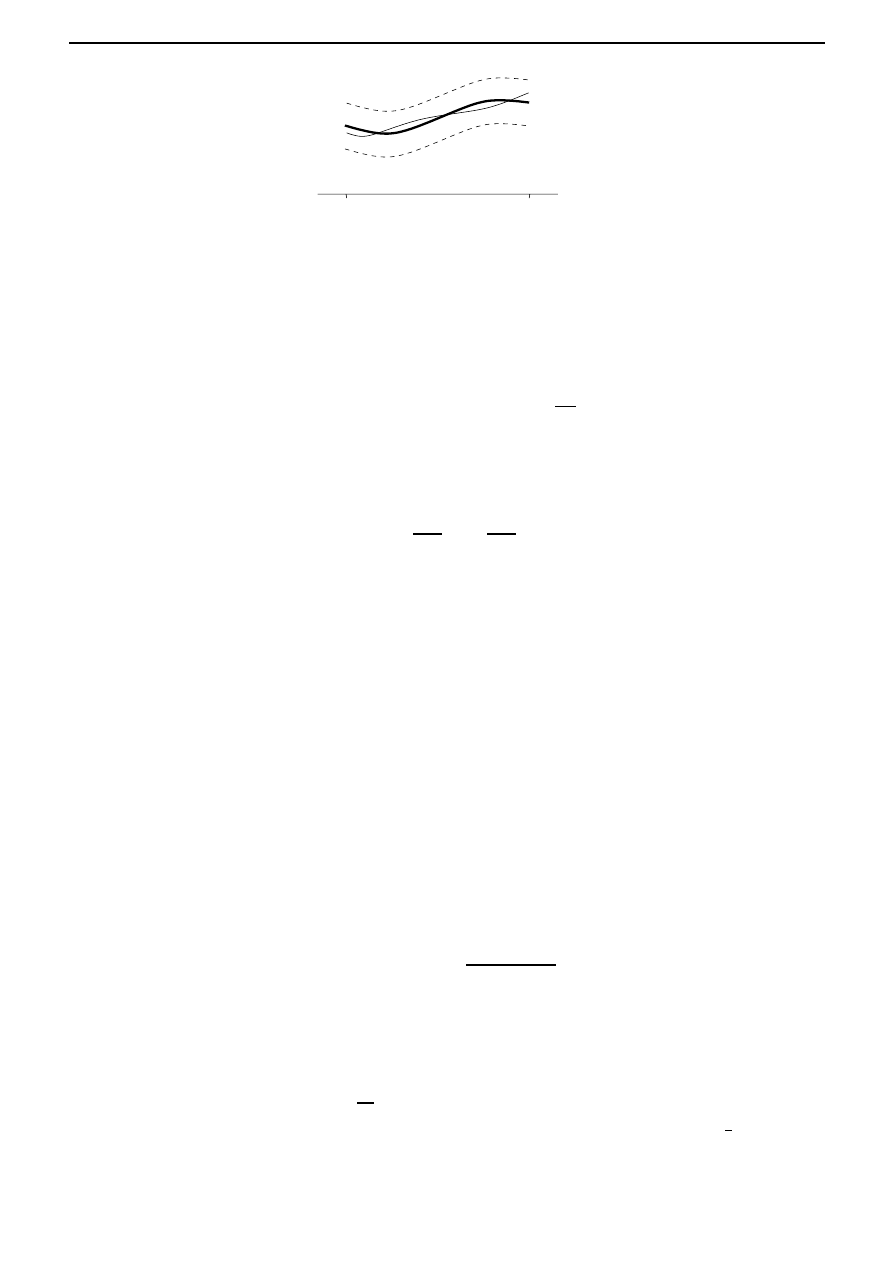
Thus in the space C[t
i
, t
f
], the distance between the function x
∗
and the function x does not
exceed if the graph of the function x lies inside a strip of width 2 ‘bordering’ the graph
of the function x
∗
, as shown in Figure 3.4.
2. C
1
[t
i
, t
f
].
20
Chapter 3. Calculus of variations
t
i
t
f
x
∗
x
t
Figure 3.4: A ball of radius and center x
∗
in C[t
i
, t
f
].
The space C
1
[t
i
, t
f
] consists of all functions x(
·) defined on [t
i
, t
f
] which are continuous and
have a continuous first derivative. The operations of addition and multiplication by scalars
are the same as in C[t
i
, t
f
], but the norm is defined by
x = max
t∈[t
i
,t
f
]
|x(t)| + max
t∈[t
i
,t
f
]
dx
dt
(t)
.
Thus two functions in C
1
[t
i
, t
f
] are regarded as close together if both the functions themselves
as well as their first derivatives are close together. Indeed this is because
x
1
−x
2
< implies
that
|x
1
(t)
− x
2
(t)
| < and
dx
1
dt
(t)
−
dx
2
dt
(t)
< for all t ∈ [t
i
, t
f
],
(3.6)
and conversely, (3.6) implies that
x
1
− x
2
< 2.
Similarly for d
∈ N, we can introduce the spaces (C[t
i
, t
f
])
d
, (C
1
[t
i
, t
f
])
d
, the spaces of functions
from [t
i
, t
f
] into
R
d
, whose each component belongs to C[t
i
, t
f
], C
1
[t
i
, t
f
], respectively.
After a norm has been introduced in a linear space X (which may be a function space), it is
natural to talk about continuity of functionals defined on X. The functional I : X
→ R is said to
be continuous at the point x
∗
if for every > 0, there exists a δ > 0 such that
|I(x) − I(x
∗
)
| < for all x such that x − x
∗
< δ.
The functional I : X
→ R is said to be continuous if it is continuous at all x ∈ X.
Exercises.
1. (
∗) Show that the arclength functional I : C
1
[0, 1]
→ R given by
I(x) =
1
0
1 + (x
(t))
2
dt
is not continuous if we equip C
1
[0, 1] with any of the following norms:
(a)
x = max
t∈[0,1]
|x(t)|, x ∈ C
1
[0, 1].
(b)
x = max
t∈[0,1]
|x(t)| +
dx
dt
(t)
.
Hint: One might proceed as follows: consider the curves x
(t) =
2
sin
t
for > 0,
and prove that
x
→ 0, while I(x
)
→ ∞ as → 0.
2. Prove that any norm defined on a linear space X is a continuous functional.
Hint: Prove that
x
− y
≤
x
− y for all x, y in X.
3.4. Calculus in function spaces and beyond
21
At first it might seem that the space C[t
i
, t
f
] (which is strictly larger than C
1
[t
i
, t
f
]) would
be adequate for the study of variational problems. However, this is not true. In fact one of the
basic functionals
I(x) =
t
f
t
i
F
x(t),
dx
dt
(t), t
dt
is continuous if we interpret closeness of functions as closeness in the space C
1
[t
i
, t
f
]. For example,
arc length is continuous if we use the norm in C
1
[t
i
, t
f
], but not
1
continuous if we use the norm
in C[t
i
, t
f
]. Since we want to be able to use ordinary analytic operations such as passage to the
limit, then, given a functional, it is reasonable to choose a function space such that the functional
is continuous.
So far we have talked about linear spaces and functionals defined on them. However, in
many variational problems, we have to deal with functionals defined on sets of functions which
do not form linear spaces. In fact, the set of functions satisfying the constraints of a given
variational problem, called the admissible functions is in general not a linear space. For example,
the admissible curves for the brachistochrone problem are the smooth plane curves passing through
two fixed points, and the sum of two such curves does not in general pass through the two points.
Nevertheless, the concept of a normed linear space and the related concepts of the distance between
functions, continuity of functionals, etcetera, play an important role in the calculus of variations.
A similar situation is encountered in elementary analysis, where, in dealing with functions of n
variables, it is convenient to use the concept of the n-dimensional Euclidean space
R
n
, even though
the domain of definition of a function may not be a linear subspace of
R
n
.
Next we introduce the concept of the (Frech´
et) derivative of a functional, analogous to the
concept of the derivative of a function of n variables. This concept will then be used to find
extrema of functionals.
Recall that for a function f :
R → R, the derivative at a point x
∗
is the approximation of f
around x
∗
by an affine linear map. See Figure 3.5.
f (x
∗
)
x
∗
x
Figure 3.5: The derivative of f at x
∗
.
In other words,
f (x
∗
+ h) = f (x
∗
) + f
(x
∗
)h + (h)
|h|
with (h)
→ 0 as |h| → 0. Here the derivative f
(x
∗
) :
R → R is simply the linear map of
multiplication. Similarly in the case of a functional I :
R
n
→ R, the derivative at a point is a
linear map I
(x
∗
) :
R
n
→ R such that
I(x
∗
+ h) = I(x
∗
) + (I
(x
∗
))(h) + (h)
h,
with (h)
→ 0 as h → 0. A linear map L : R
n
→ R is always continuous. But this is not true in
general if
R
n
is replaced by an infinite dimensional normed linear space X. So while generalizing
1
For every curve, we can find another curve arbitrarily close to the first in the sense of the norm of
C[t
i
, t
f
],
whose length differs from that of the first curve by a factor of 10, say.

22
Chapter 3. Calculus of variations
the notion of the derivative of a functional I : X
→ R, we specify continuity of the linear map
as well. This motivates the following definition. Let X be a normed linear space. Then a map
L : X
→ R is said to be a continuous linear functional if it is linear and continuous.
Exercises.
1. Let L : X
→ R be a linear functional on a normed linear space X. Prove that the following
are equivalent:
(a) L is continuous.
(b) L is continuous at 0.
(c) There exists a M > 0 such that
|L(x)| ≤ Mx for all x ∈ X.
Hint. The implication (1a)
⇒(1b) follows from the definition and (1c)⇒(1a) is easy to prove
using a δ <
M
. For (1b)
⇒(1c), use M >
δ
and consider separately the cases x = 0 and
x
= 0. In the latter case, note that with x
1
:=
M
x
x, there holds that
x
1
< δ.
Remark. Thus in the case of
linear functionals, remarkably, continuity is equivalent to
continuity at only one point, and this is furthermore equivalent to proving an estimate of
the type given in item 1c.
2. Let t
m
∈ [t
i
, t
f
]. Prove that the map L : C[t
i
, t
f
]
→ R given by L(x) = x(t
m
) is a continuous
linear functional.
3. Let α, β
∈ C[t
i
, t
f
]. Prove that the map L : C
1
[t
i
, t
f
]
→ R given by
L(x) =
t
f
t
i
α(t)x(t) + β(t)
dx
dt
(t)
dt
is a continuous linear functional.
We are now ready to define the derivative of a functional. Let X be a normed linear space
and I : X
→ R be a functional. Then I is said to be (Frech´et) differentiable at x
∗
(
∈ X) if there
exists a continuous linear functional, denoted by I
(x
∗
), and a map : X
→ R such that
I(x
∗
+ h) = I(x
∗
) + (I
(x
∗
))(h) + (h)
h, for all h ∈ X,
and (h)
→ 0 as h → 0. Then I
(x
∗
) is called the (Frech´
et) derivative of I at x
∗
. If I is
differentiable at every point x
∈ X, then it is simply said to be differentiable.
Theorem 3.4.1
The derivative of a differentiable functional I : X
→ R at a point x
∗
(
∈ X) is
unique.
Proof First we note that if
L : X
→ R is a linear functional and if
L(h)
h
→ 0 as h → 0,
(3.7)
then L = 0. For if L(h
0
)
= 0 for some nonzero h
0
∈ X, then defining h
n
=
1
n
h
0
, we see that
h
n
→ 0 as n → ∞, but
lim
n→∞
L(h
n
)
h
n
=
D(h
0
)
h
0
= 0,

3.4. Calculus in function spaces and beyond
23
which contradicts (3.7).
Now suppose that the derivative of I at x
∗
is not uniquely defined, so that
I(x
∗
+ h)
=
I(x
∗
) + L
1
(h) +
1
(h)
h,
I(x
∗
+ h)
=
I(x
∗
) + L
2
(h) +
2
(h)
h,
where L
1
, L
2
are continuous linear functionals, and
1
(h),
2
(h)
→ 0 as h → 0. Thus
(L
1
− L
2
)(h)
h
=
2
(h)
−
1
(h)
→ 0 as h → 0,
and from the above, it follows that L
1
= L
2
.
Exercises.
1. Prove that if I : X
→ R is differentiable at x
∗
, then it is continuous at x
∗
.
2.
(a) Prove that if L : X
→ R is a continuous linear functional, then it is differentiable.
What is its derivative at x
∈ X?
(b) Let t
m
∈ [t
i
, t
f
]. Consider the functional I : C[t
i
, t
f
]
→ R given by
I(x) =
t
f
t
m
x(t)dt.
Prove that I is differentiable, and find its derivative at x
∈ C[t
i
, t
f
].
3. (
∗) Prove that the square of a differentiable functional I : X → R is differentiable, and find
an expression for its derivative at x
∈ X.
4.
(a) Given x
1
, x
2
in a normed linear space X, define
ϕ(t) = tx
1
+ (1
− t)x
2
.
Prove that if I : X
→ R is differentiable, then I ◦ ϕ : [0, 1] → R is differentiable and
d
dt
(I
◦ ϕ)(t) = [I
(ϕ(t))](x
1
− x
2
).
(b) Prove that if I
1
, I
2
: X
→ R are differentiable and their derivatives are equal at every
x
∈ X, then I
1
, I
2
differ by a constant.
In elementary analysis, a necessary condition for a differentiable function f :
R → R to have
a local extremum (local maximum or local minimum) at x
∗
∈ R is that f
(x
∗
) = 0. We will
prove a similar necessary condition for a differentiable functional I : X
→ R. We say that a
functional I : X
→ R has a local extremum at x
∗
(
∈ X) if I(x) − I(x
∗
) does not change sign in
some neighbourhood of x
∗
.
Theorem 3.4.2
Let I : X
→ R be a functional that is differentiable at x
∗
∈ X. If I has a local
extremum at x
∗
, then I
(x
∗
) = 0.
Proof
To be explicit, suppose that I has a minimum at x
∗
: there exists r > 0 such that
I(x
∗
+ h)
≥ I(x
∗
) for all h such that
h < r. Suppose that [I
(x
∗
)](h
0
)
= 0 for some h
0
∈ X.
Define
h
n
=
−
1
n
[I
(x
∗
)](h
0
)
|[I
(x
∗
)](h
0
)
|
h
0
.
24
Chapter 3. Calculus of variations
We note that
h
n
→ 0 as n → ∞, and so with N chosen large enough, we have h
n
< r for all
n > N . It follows that for n > N ,
0
≤
I(x
∗
+ h
n
)
− I(x
∗
)
h
n
=
−
|[I
(x
∗
)](h
0
)
|
h
0
+ (h
n
).
Passing the limit as n
→ ∞, we obtain −|[I
(x
∗
)](h
0
)
| ≥ 0, a contradiction.
Remark. Note that this is a
necessary condition for the existence of an extremum. Thus a the
vanishing of a derivative at some point x
∗
doesn’t imply extremality of x
∗
!
3.5
The simplest variational problem. Euler-Lagrange equa-
tion
The simplest variational problem can be formulated as follows:
Let F (
x, x
,
t) be a function with continuous first and second partial derivatives with respect to
(
x, x
,
t). Then find x ∈ C
1
[t
i
, t
f
] such that x(t
i
) = x
i
and x(t
f
) = x
f
, and which is an extremum
for the functional
I(x) =
t
f
t
i
F
x(t),
dx
dt
(t), t
dt.
(3.8)
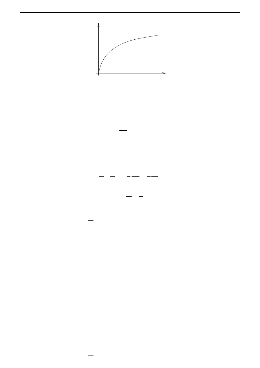
In other words, the simplest variational problem consists of finding an extremum of a functional
of the form (3.13), where the class of admissible curves comprises all smooth curves joining two
fixed points; see Figure 3.6. We will apply the necessary condition for an extremum (established
t
i
t
f
t
x
i
x
f
Figure 3.6: Possible paths joining the two fixed points (t
i
, x
i
) and (t
f
, x
f
).
in Theorem 3.4.2) to the solve the simplest variational problem described above. This will enable
us to solve the brachistochrone problem from
§3.2.
Theorem 3.5.1
Let I be a functional of the form
I(x) =
t
f
t
i
F
x(t),
dx
dt
(t), t
dt,
where F (
x, x
,
t) is a function with continuous first and second partial derivatives with respect to
(
x, x
,
t) and x ∈ C
1
[t
i
, t
f
] such that x(t
i
) = x
i
and x(t
f
) = x
f
. If I has an extremum at x
∗
, then
x
∗
satisfies the Euler-Lagrange equation:
∂F
∂
x
x
∗
(t),
dx
∗
dt
(t), t
−
d
dt
∂F
∂
x
x
∗
(t),
dx
∗
dt
(t), t
= 0, t
∈ [t
i
, t
f
].
(3.9)

3.5. The simplest variational problem. Euler-Lagrange equation
25
(This equation is abbreviated by F
x
−
d
dt
F
x
= 0.)
Proof The proof is long and so we divide it into several steps.
Step 1. First of all we note that the set of curves in C
1
[t
i
, t
f
] satisfying x(t
i
) = x
i
and x(t
f
) = x
f
do not form a linear space! So Theorem 3.4.2 is not applicable directly. Hence we introduce a
new linear space X, and consider a new functional ˜
I : X
→ R which is defined in terms of the old
functional I.
Introduce the linear space
X =
{h ∈ C
1
[t
i
, t
f
]
| h(a) = h(b) = 0},
with the C
1
[t
i
, t
f
]-norm. Then for all h
∈ X, x
∗
+h satisfies (x
∗
+h)(t
i
) = x
i
and (x
∗
+h)(t
f
) = x
f
.
Defining ˜
I(h) = I(x
∗
+h), we note that ˜
I : X
→ R has an extremum at 0. It follows from Theorem
3.4.2 that ˜
I
(0) = 0. Note that by the 0 in the right hand side of the equality, we mean the zero
functional, namely the continuous linear map from X to
R, which is defined by h → 0 for all
h
∈ X.
Step 2. We now calculate ˜I
(0). We have
˜
I(h)
− ˜I(0) =
t
f
t
i
F ((x
∗
+ h)(t), (x
∗
+ h)
(t), t) dt
−
t
f
t
i
F (x
∗
(t), x
∗
(t), t) dt
=
t
f
t
i
[F (x
∗
(t) + h(t), x
∗
(t) + h
(t), t) dt
− F (x
∗
(t), x
∗
(t), t)] dt.
Recall that from Taylor’s theorem, if F possesses partial derivatives of order 2 in some neighbour-
hood N of (x
0
, x
0
, t
0
), then for all (x, x
, t)
∈ N, there exists a Θ ∈ [0, 1] such that
F (x, x
, t)
=
F (x
0
, x
0
, t
0
) +
(x
− x
0
)
∂
∂
x
+ (x
− x
0
)
∂
∂
x
+ (t
− t
0
)
∂
∂
t
F
(x
0
,x
0
,t
0
)
+
1
2!
(x
− x
0
)
∂
∂
x
+ (x
− x
0
)
∂
∂
x
+ (t
− t
0
)
∂
∂
t
2
F
(x
0
,x
0
,t
0
)+Θ
(
(x,x
,t)−(x
0
,x
0
,t
0
)
)
.
Hence for h
∈ X such that h is small enough,
˜
I(h)
− ˜I(0) =
t
f
t
i
∂F
∂
x
(x
∗
(t), x
∗
(t), t) h(t) +
∂F
∂
x
(x
∗
(t), x
∗
(t), t) h
(t)
dt +
1
2!
t
f
t
i
h(t)
∂
∂
x
+ h
(t)
∂
∂
x
2
F
(x
∗
(t)+Θ(t)h(t),x
∗
(t)+Θ(t)h
(t),t)
dt.
It can be checked that there exists a M > 0 such that
1
2!
t
f
t
i
h(t)
∂
∂
x
+ h
(t)
∂
∂
x
2
F
(x
∗
(t)+Θ(t)h(t),x
∗
(t)+Θ(t)h
(t),t)
dt
≤ Mh
2
,
and so ˜
I
(0) is the map
h
→
t
f
t
i
∂F
∂
x
(x
∗
(t), x
∗
(t), t) h(t) +
∂F
∂
x
(x
∗
(t), x
∗
(t), t) h
(t)
dt.
(3.10)
26
Chapter 3. Calculus of variations
Step 3. Next we show that if the map in (3.10) is the zero map, then this implies that (3.9)
holds. Define
A(t) =
t
t
i
∂F
∂
x
(x
∗
(τ ), x
∗
(τ ), τ ) dτ.
Integrating by parts, we find that
t
f
t
i
∂F
∂
x
(x
∗
(t), x
∗
(t), t) h(t)dt =
−
t
f
t
i
A(t)h
(t)dt,
and so from (3.10), it follows that ˜
I
(0) = 0 implies that
t
f
t
i
−A(t) +
∂F
∂
x
(x
∗
(t), x
∗
(t), t)
h
(t)dt = 0 for all h
∈ X.
Step 4. Finally we will complete the proof by proving the following.
Lemma 3.5.2
If K
∈ C[t
i
, t
f
] and
t
f
t
i
K(t)h
(t)dt = 0
for all h
∈ C
1
[t
i
, t
f
] with h(t
i
) = h(t
f
) = 0, then there exists a constant k such that K(t) = k for
all t
∈ [t
i
, t
f
].
Proof Let
k be the constant defined by the condition
t
f
t
i
[K(t)
− k] dt = 0,
and let
h(t) =
t
t
i
[K(τ )
− k] dτ.
Then h
∈ C
1
[t
i
, t
f
] and it satisfies h(t
i
) = h(t
f
) = 0. Furthermore,
t
f
t
i
[K(t)
− k]
2
dt =
t
f
t
i
[K(t)
− k] h
(t)dt =
t
f
t
i
K(t)h
(t)dt
− k(h(t
f
)
− h(t
i
)) = 0.
Thus K(t)
− k = 0 for all t ∈ [t
i
, t
f
].
Applying Lemma 3.5.2, we obtain
−A(t) +
∂F
∂
x
(x
∗
(t), x
∗
(t), t) = k for all t
∈ [t
i
, t
f
].
Differentiating with respect to t, we obtain (3.10). This completes the proof of Theorem 3.5.1.
Since the Euler-Lagrange equation is in general a second order differential equation, it solu-
tion will in general depend on two arbitrary constants, which are determined from the boundary
conditions x(t
i
) = x
i
and x(t
f
) = x
f
. The problem usually considered in the theory of differen-
tial equations is that of finding a solution which is defined in the neighbourhood of some point
and satisfies given initial conditions (Cauchy’s problem). However, in solving the Euler-Lagrange
equation, we are looking for a solution which is defined over all of some fixed region and satisfies
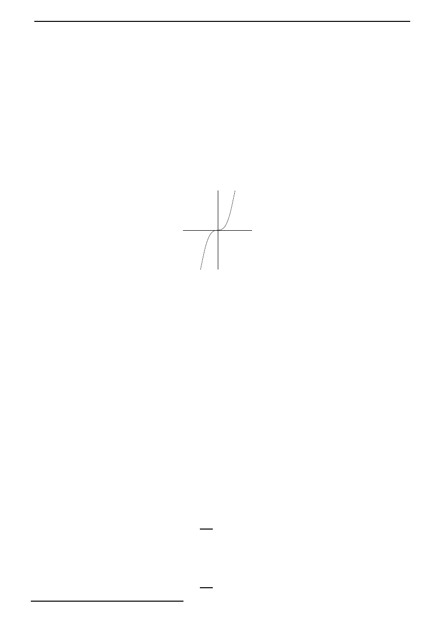
3.5. The simplest variational problem. Euler-Lagrange equation
27
given boundary conditions. Therefore, the question of whether or not a certain variational problem
has a solution does not just reduce to the usual existence theorems for differential equations.
Note that the Euler-Lagrange equation is only a necessary condition for the existence of an
extremum. This is analogous to the case of f :
R → R given by f(x) = x
3
, for which f
(0) = 0,
although f clearly does not have a minimum or maximum at 0. See Figure 3.7 and also the
Exercise 1 on page 27. However, in many cases, the Euler-Lagrange equation by itself is enough to
give a complete solution of the problem. In fact, the existence of an extremum is sometimes clear
from the context of the problem. From example, in the brachistochrone problem, it is clear from
the physical meaning. Similarly in the problem concerning finding the curve with the shortest
distance between two given points, this is clear from the geometric meaning. If in such scenarios,
there exists only one critical curve
2
satisfying the boundary conditions of the problem, then this
critical curve must a fortiori be the curve for which the extremum is achieved.
x
y = x
3
y
0
Figure 3.7: The derivative vanishes at 0, although it is not a point at which the function has a
maximum or a minimum.
The Euler-Lagrange equation is in general a second order differential equation, but in some
special cases, it can be reduced to a first order differential equation or where its solution can be
obtained entirely by evaluating integrals. We indicate some special cases in Exercise 2 on page ,
where in each instance, F is independent of one of its arguments.
Exercises.
1. Consider the functional I given by
I(x) =
1
0
(x(t))
3
dt,
defined for all x
∈ C
1
[0, 1] with x(0) = 0 = x(1). Using Theorem 3.5.1, find the critical
curve x
∗
for this functional. Is this a curve which maximizes or minimizes the functional I?
2. Prove that:
(a) If F does not depend in
x, then the Euler-Lagrange equation becomes
∂F
∂
x
(x(t), x
(t), t) = c,
where c is a constant.
(b) If F does not depend in
x
, then the Euler-Lagrange equation becomes
∂F
∂
x
(x(t), x
(t), t) = 0.
2
The solutions of the Euler-Lagrange equation are called critical curves.
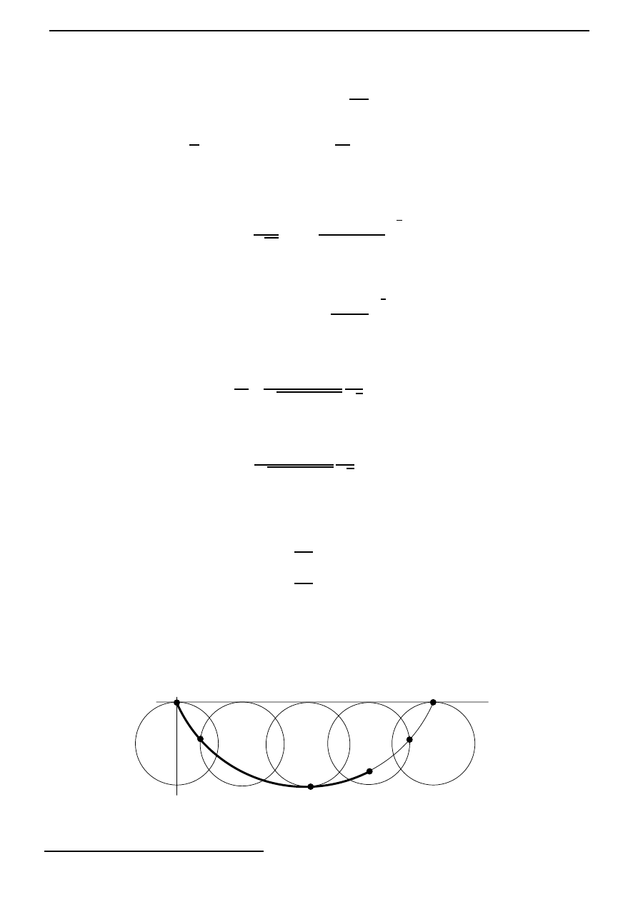
28
Chapter 3. Calculus of variations
(c) If F does not depend in
t and if x
∗
∈ C
2
[t
i
, t
f
], then the Euler-Lagrange equation
becomes
F (x(t), x
(t), t)
− x
(t)
∂F
∂
x
(x(t), x
(t), t) = c,
where c is a constant.
Hint: What is
d
dt
F (x(t), x
(t), t)
− x
(t)
∂F
∂x
(x(t), x
(t), t)
?
Example.
(Brachistochrone problem, continued.) Determine the minimum value of the functional
I(y) =
1
√
2g
x
0
0
1 + (x
(y))
2
y
1
2
dy,
with x
∈ C
1
[0, y
0
] and x(0) = 0, x(y
0
) = x
0
. Here
3
F (
x, x
,
t) =
1 +
x
2
t
1
2
is independent of
x, and so the Euler-Lagrange equation becomes
d
dy
x
(y)
1 + (x
(y))
2
1
√
y
= 0.
Integrating with respect to y, we obtain
x
(y)
1 + (x
(y))
2
1
√
y
= c,
where c is a constant. It can be shown that the general solution of this differential equation is
given by
x(Θ)
=
1
2c
2
(Θ
− sin Θ) + ˜c,
y(Θ)
=
1
2c
2
(1
− cos Θ),
where ˜
c is another constant. The constants are chosen so that the curve passes through the points
(0, 0) and (x
0
, y
0
). This curve is known as a cycloid, and in fact it is the curve described by a
point P in a circle that rolls without slipping on the x axis, in such a way that P passes through
(x
0
, y
0
); see Figure 3.8.
(0, 0)
(x
0
, y
0
)
x
y
Figure 3.8: The cycloid through (0, 0) and (x
0
, y
0
).
3
Strictly speaking, the
F here does not satisfy the demands made in Theorem 3.5.1. Notwithstanding this fact,
with some additional argument, the solution given here can be fully justified.
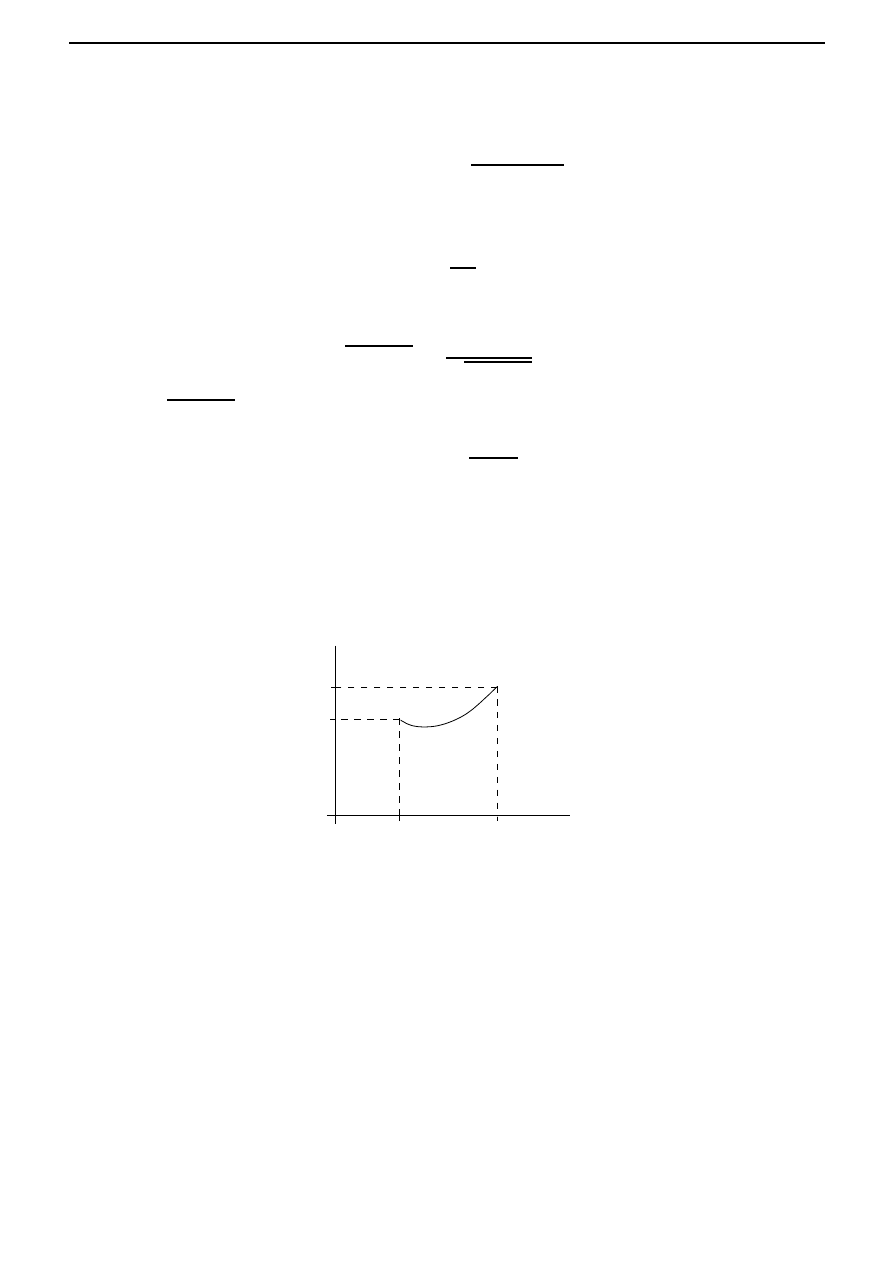
3.5. The simplest variational problem. Euler-Lagrange equation
29
Example. Among all the curves joining two given points (
x
0
, y
0
) and (x
1
, y
1
), find the one which
generates the surface of minimum area when rotated about the x axis. The area of the surface of
revolution generated by rotating the curve y about the x axis is
S(y) = 2π
x
1
x
0
y(x)
1 + (y
(x))
2
dx.
Since the integrand does not depend explicitly on x, the Euler-Lagrange equation is
F (y(x), y
(x), x)
− y
(x)
∂F
∂
y
(y(x), y
(x), x) = c,
where c is a constant, that is,
y
1 + (y
)
2
− y
(y
)
2
1 + (y
)
2
= c.
Thus y = c
1 + (y
)
2
, and it can be shown that this differential equation has the general solution
y(x) = c cosh
x + c
1
c
.
(3.11)
This curve is called a catenary. The values of the arbitrary constants c and c
1
are determined
by the conditions y(x
0
) = y
0
and y(x
1
) = y
1
. It can be shown that the following three cases are
possible, depending on the positions of the points (x
0
, y
0
) and (x
1
, y
1
):
1. If a single curve of the form (3.11) passes through the points (x
0
, y
0
) and (x
1
, y
1
), then this
curve is the solution of the problem; see Figure 3.9.
x
0
x
1
y
0
y
1
Figure 3.9: The catenary through (x
0
, y
0
) and (x
1
, y
1
).
2. If two critical curves can be drawn through the points (x
0
, y
0
) and (x
1
, y
1
), then one of the
curves actually corresponds to the surface of revolution if minimum area, and the other does
not.
3. If there does not exist a curve of the form (3.11) passing through the points (x
0
, y
0
) and
(x
1
, y
1
), then there is no surface in the class of smooth surfaces of revolution which achieves
the minimum area. In fact, if the location of the two points is such that the distance between
them is sufficiently large compared to their distances from the x axis, then the area of the
surface consisting of two circles of radius y
0
and y
1
will be less than the area of any surface of
revolution generated by a smooth curve passing through the points; see Figure 3.10. This is
intuitively expected: imagine a soap bubble between concentric rings which are being pulled
apart. Intially we get a soap bubble between these rings, but if the distance separating the
rings becomes too large, then the soap bubble breaks, leaving a soap films on each of the two
rings. This example shows that a critical curve need not always exist in the class of curves
under consideration.
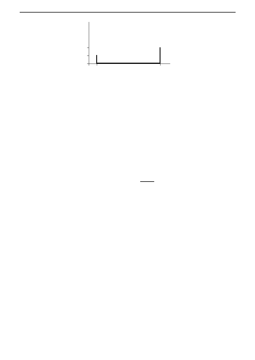
30
Chapter 3. Calculus of variations
x
0
x
1
y
0
y
1
Figure 3.10: The polygonal curve (x
0
, y
0
)
− (x
0
, 0)
− (x
1
, 0)
− (x
1
, y
1
).
Exercises.
1. Find the curve which has minimum length between (0, 0) and (1, 1).
2. Find critical curves for the following functionals, where in each case x(0) = 0 and x(1) = 1:
(a) I(x) =
1
0
x
(t)dt.
(b) I(x) =
1
0
x(t)x
(t)dt.
(c) I(x) =
1
0
(x(t) + tx
(t))dt. (See the Exercise on page 2.3.)
3. Find critical curves for the functional I(x) =
2
1
t
3
(x
(t))
2
dt where x(1) = 5 and x(2) = 2.
4. Find critical curves for the functional I(x) =
2
1
(x
(t))
3
t
2
dt where x(1) = 1 and x(2) = 7.
5. Find critical curves for the functional I(x) =
1
0
2tx(t)
− (x
(t))
2
+ 3x
(t)(x(t))
2
dt where
x(0) = 0 and x(1) =
−1.
6. Find critical curves for the functional I(x) =
1
0
2(x(t))
3
+ 3t
2
x
(t)
dt where x(0) = 0 and
x(1) = 1. What if x(0) = 0 and x(1) = 2?
7. A strip-mining company intends to remove all of the iron ore from a region that contains
an estimated Q tons over a fixed time interval [0, T ]. As it is extracted, they will sell it for
processing at a net price per ton of
p(x(t), x
(t)) = P
− αx(t) − βx
(t)
for positive constants P , α, and β, where x(t) denotes the total tonnage sold by time t. (This
pricing model allows the cost of mining to increase with the extent of the mined region and
speed of production.)
(a) If the company wishes to maximize its total profit given by
I(x) =
T
0
p(x(t), x
(t))x
(t)dt,
(3.12)
where x(0) = 0 and x(T ) = Q, how might it proceed?
(b) If future money is discounted continuously at a constant rate r, then we can assess the
present value of profits from this mining operation by introducing a factor of e
−rt
in
the integrand of (3.12). Suppose that α = 4, β = 1, r = 1 and P = 2. Find an optimal
mining operation.
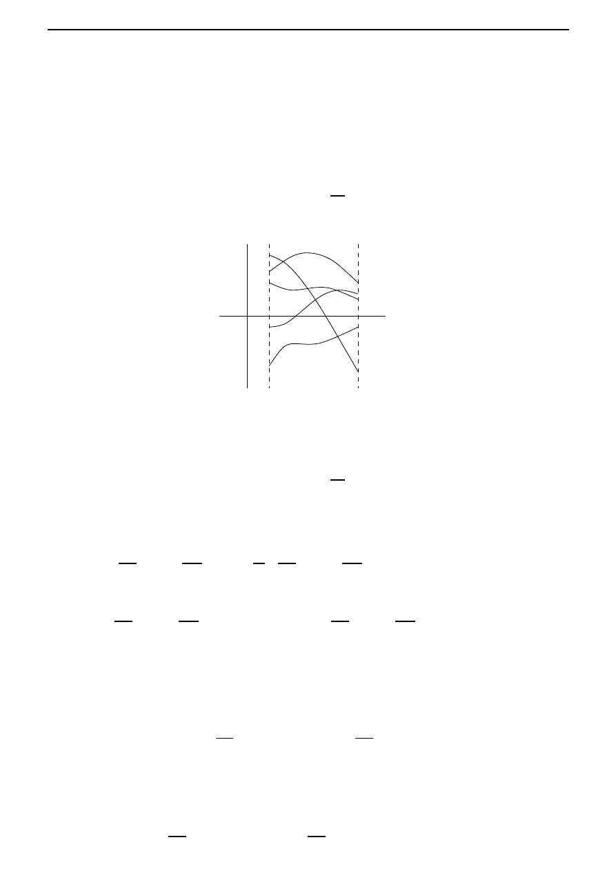
3.6. Free boundary conditions
31
3.6
Free boundary conditions
Besides the simplest variational problem considered in the previous section, we now consider the
variational problem with free boundary conditions (see Figure 3.11):
Let F (
x, x
,
t) be a function with continuous first and second partial derivatives with respect to
(
x, x
,
t). Then find x ∈ C
1
[t
i
, t
f
] which is an extremum for the functional
I(x) =
t
f
t
i
F
x(t),
dx
dt
(t), t
dt.
(3.13)
t
i
t
f
t
Figure 3.11: Free boundary conditions.
Theorem 3.6.1
Let I be a functional of the form
I(x) =
t
f
t
i
F
x(t),
dx
dt
(t), t
dt,
where F (
x, x
,
t) is a function with continuous first and second partial derivatives with respect to
(
x, x
,
t) and x ∈ C
1
[t
i
, t
f
]. If I has an extremum at x
∗
, then x
∗
satisfies the Euler-Lagrange
equation:
∂F
∂
x
x
∗
(t),
dx
∗
dt
(t), t
−
d
dt
∂F
∂
x
x
∗
(t),
dx
∗
dt
(t), t
= 0, t
∈ [t
i
, t
f
],
(3.14)
together with the transversality conditions
∂F
∂
x
x
∗
(t),
dx
∗
dt
(t), t
t=t
i
= 0
and
∂F
∂
x
x
∗
(t),
dx
∗
dt
(t), t
t=t
f
= 0.
(3.15)
Proof
Step 1. We take X = C
1
[t
i
, t
f
] and compute I
(x
∗
). Proceeding as in the proof of Theorem 3.5.1,
it is easy to see that
(I
(x
∗
))(h) =
t
f
t
i
∂F
∂
x
(x
∗
(t), x
∗
(t), t) h(t) +
∂F
∂
x
(x
∗
(t), x
∗
(t), t) h
(t)
dt,
h
∈ C
1
[t
i
, t
f
]. Theorem 3.4.2 implies that this linear functional must be the zero map, that is,
(I
(x
∗
))(h) = 0 for all h
∈ C
1
[t
i
, t
f
]. In particular, it is also zero for all h in C
1
[t
i
, t
f
] such that
h(t
i
) = h(t
f
) = 0. But recall that in
Step 3 and Step 4 of the proof of Theorem 3.5.1, we proved
that if
t
f
t
i
∂F
∂
x
(x
∗
(t), x
∗
(t), t) h(t) +
∂F
∂
x
(x
∗
(t), x
∗
(t), t) h
(t)
dt = 0
(3.16)

32
Chapter 3. Calculus of variations
for all h in C
1
[t
i
, t
f
] such that h(t
i
) = h(t
f
) = 0, then this implies that he Euler-Lagrange equation
(3.14) holds.
Step 2. Integration by parts in (3.16) now gives
(I
(x
∗
))(h)
=
t
f
t
i
∂F
∂
x
(x
∗
(t), x
∗
(t), t)
−
d
dt
∂F
∂
x
(x
∗
(t), x
∗
(t), t)
h(t)dt +
(3.17)
∂F
∂
x
(x
∗
(t), x
∗
(t), t) h(t)
t=t
f
t=t
i
=
0 +
∂F
∂
x
(x
∗
(t), x
∗
(t), t)
t=t
f
h(t
f
)
−
∂F
∂
x
(x
∗
(t), x
∗
(t), t)
t=t
i
h(t
i
).
The integral in (3.17) vanishes since we have shown in
Step 1 above that (3.14) holds. Thus the
condition I
(x
∗
) = 0 now takes the form
∂F
∂
x
(x
∗
(t), x
∗
(t), t)
t=t
f
h(t
f
)
−
∂F
∂
x
(x
∗
(t), x
∗
(t), t)
t=t
i
h(t
i
) = 0,
from which (3.15) follows, since h is arbitrary. This completes the proof.
Exercises.
1. Find all curves y = y(x) which have minimum length between the lines x = 0 and the line
x = 1.
2. Find critical curves for the following functional, when the values of x are free at the endpoints:
I(x) =
1
0
1
2
(x
(t))
2
+ x(t)x
(t) + x
(t) + x(t)
dt.
Similarly, we can also consider the mixed case (see Figure 3.12), when one end of the curve is
fixed, say x(t
i
) = x
i
, and the other end is free. Then it can be shown that the curve x satisfies
the Euler-Lagrange equation, the transversality condition
∂F
∂
x
(x
∗
(t), x
∗
(t), t)
t=t
i
h(t
i
) = 0
at the free end point, and x(t
i
) = x
i
serves as the other boundary condition.
We can summarize the results by the following: critical curves for (3.13) satisfy the Euler-
Lagrange equation (3.14) and moreover there holds
∂F
∂
x
(x
∗
(t), x
∗
(t), t) = 0 at the free end point.
Exercises.
1. Find the curve y = y(x) which has minimum length between (0, 0) and the line x = 1.
2. Find critical curves for the following functionals:
(a) I(x) =
π
2
0
(x(t))
2
− (x
(t))
2
dt, x(0) = 0 and x
π
2
is free.
(b) I(x) =
π
2
0
(x(t))
2
− (x
(t))
2
dt, x(0) = 1 and x
π
2
is free.
(c) I(x) =
1
0
cos(x
(t))dt, x(0) = 0 and x(1) is free.
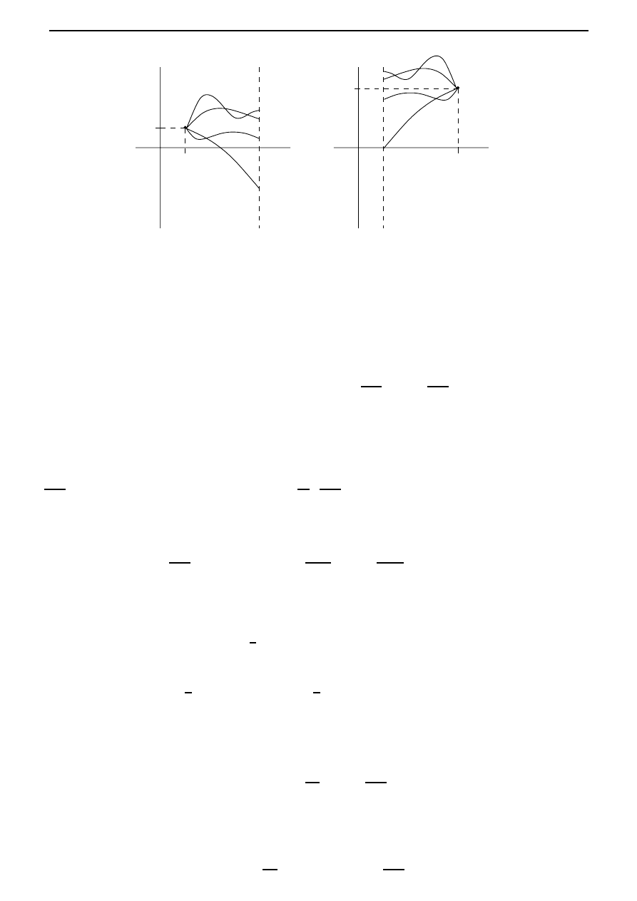
3.7. Generalization
33
t
i
t
i
t
f
t
f
x
i
x
f
t
t
Figure 3.12: Mixed cases.
3.7
Generalization
The results in this chapter can be generalized to the case when the integrand F is a function of
more than one independent variable: if we wish to find extremum values of the functional
I(x
1
, . . . , x
n
) =
t
f
t
i
F
x
1
(t), . . . , x
n
(t),
dx
1
dt
(t), . . . ,
dx
n
dt
(t), t
dt,
where F (
x
1
, . . . ,
x
n
,
x
1
, . . . ,
x
n
,
t) is a function with continuous partial derivatives of order ≤ 2,
and x
1
, . . . , x
n
are independent functions of the variable t, then following a similar analysis as
before, we obtain n Euler-Lagrange equations to be satisfied by the optimal curve, that is,
∂F
∂
x
k
(x
1∗
(t), . . . , x
n∗
(t), x
1∗
(t), . . . , x
n∗
(t), t)
−
d
dt
∂F
∂
x
k
(x
1∗
(t), . . . , x
n∗
(t), x
1∗
(t), . . . , x
n∗
(t), t)
= 0,
for t
∈ [t
i
, t
f
], k
∈ {1, . . . , n}. Also at any end point where x
k
is free,
∂F
∂
x
k
x
1∗
(t), . . . , x
n∗
(t),
dx
1∗
dt
(t), . . . ,
dx
n∗
dt
(t), t
= 0.
Exercise. Find critical curves of the functional
I(x
1
, x
2
) =
π
2
0
(x
1
(t))
2
+ (x
2
(t))
2
+ 2x
1
(t)x
2
(t)
dt
such that x
1
(0) = 0, x
1
π
2
= 1, x
2
(0) = 0, x
2
π
2
= 1.
Remark. Note that with the above result, we can also solve the problem of finding extremal
curves for a functional of the type
I(x) :
t
f
t
i
F
x(t),
dx
dt
(t), . . . ,
d
n
x
dt
n
(t), t
dt,
for over all (sufficiently differentiable) curves x defined on an interval [t
i
, t
f
], taking values in
R.
Indeed, we may introduce the auxiliary functions
x
1
(t) = x(t), x
2
(t) =
dx
dt
(t), . . . , x
n
(t) =
d
n
x
dt
n
(t),
t
∈ [t
i
, t
f
],

34
Chapter 3. Calculus of variations
and consider the problem of finding extremal curves for the new functional ˜
I defined by
˜
I(x
1
, . . . , x
n
) =
t
f
t
i
F (x
1
(t), x
2
(t), . . . , x
n
(t), t)dt.
Using the result mentioned in this section, we can then solve this problem. Note that we eliminated
high order derivatives at the price of converting the scalar function into a vector-valued function.
Since we can always do this, this is one of the reasons in fact for considering functionals of the
type (3.2) where no high order derivatives occur.

Chapter 4
Optimal control
4.1
The simplest optimal control problem
In this section, we wish to find the functions u that give extremum values of
I
x
i
(u) =
t
f
t
i
F (x(t), u(t), t)dt,
where x is the unique solution of the differential equation
˙x(t) = f (x(t), u(t)), t
∈ [t
i
, t
f
], x(t
i
) = x
i
.
We prove the following result.
Theorem 4.1.1
Let F (
x, u, t) and f(x, u) be continuously differentiable functions of each of their
arguments. Suppose that u
∗
∈ C[t
i
, t
f
] is an optimal control for the functional I
x
i
: C[t
i
, t
f
]
→ R
defined as follows: If u
∈ C[t
i
, t
f
], then
I
x
i
(u) =
t
f
t
i
F (x(t), u(t), t)dt,
where x(
·) denotes the unique solution to the differential equation
˙x(t) = f (x(t), u(t)), t
∈ [t
i
, t
f
], x(t
i
) = x
i
.
(4.1)
If x
∗
denotes the state corresponding to the input u
∗
, then there exists a p
∗
∈ C
1
[t
i
, t
f
] such that
∂F
∂
x
(x
∗
(t), u
∗
(t), t) + p
∗
(t)
∂f
∂
x
(x
∗
(t), u
∗
(t))
=
− ˙p
∗
(t),
t
∈ [t
i
, t
f
], p
∗
(t
f
) = 0,
(4.2)
∂F
∂
u
(x
∗
(t), u
∗
(t), t) + p
∗
(t)
∂f
∂
u
(x
∗
(t), u
∗
(t))
=
0,
t
∈ [t
i
, t
f
].
(4.3)
Proof The proof can be divided into three main steps.
Step 1. In this step we consider an associated function I
ξ
2
:
R → R (defined below) that is
defined in terms of the functional I. Using the optimality of u
∗
for I, we then conclude that the
function I
ξ
2
must have an extremum at 0 (
∈ R). Thus applying the necessity of the condition
35
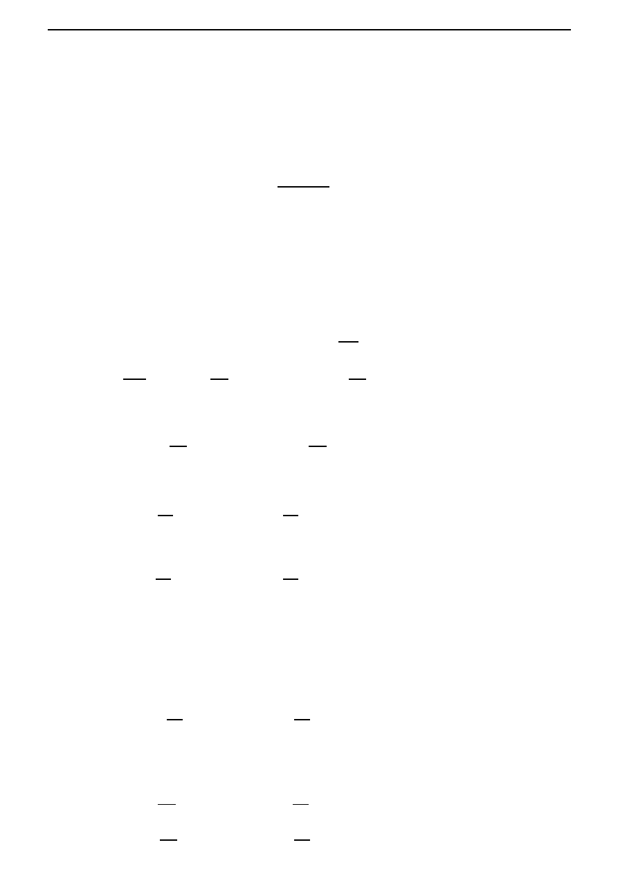
36
Chapter 4. Optimal control
that the derivative must vanish at extremal points (now simply for a function from
R to R!), we
obtain a certain condition, given by equation (4.6).
Let ξ
2
∈ C[t
i
, t
f
] be such that ξ
2
(t
i
) = ξ
2
(t
f
) = 0. Define u
(t) = u
∗
(t) + ξ
2
(t),
∈ R. Then
from Theorem 1.2.2, for all such that
|| < δ, with δ small enough, there exists a unique x
(
·)
satisfying
˙
x
(t) = f (x
(t), u
(t)), t
∈ [t
i
, t
f
], x
(t
i
) = x
i
.
(4.4)
Define ξ
1
∈ C
1
[t
i
, t
f
] by
ξ
1
(t) =
x
(t)−x
∗
(t)
if
= 0,
0
if = 0.
Then ξ
1
(t
i
) = 0, and x
(t) = x
∗
(t) + ξ
1
(t) for all
∈ (−δ, δ). Let
I
ξ
2
() =
t
f
t
i
F (x
(t), u
(t), t)dt =
t
f
t
i
F (x
∗
(t) + ξ
1
(t), u
∗
(t) + ξ
2
(t), t)dt.
It thus follows that I
ξ
2
: (
−δ, δ) → R is differentiable (differentiation under the integral sign can
be justified!), and from the hypothesis that u
∗
is optimal for I
x
i
, it follows that the function I
ξ
2
has an extremum for = 0. As a consequence of the necessity of the condition that the derivative
must vanish at extremal points, there must hold that
dI
ξ2
d
(0) = 0. But we have
dI
ξ
2
d
() =
t
f
t
i
∂F
∂
x
(x
(t), u
(t), t)ξ
1
(t) +
∂F
∂
u
(x
(t), u
(t), t)ξ
2
(t)
dt,
and so we obtain
t
f
t
i
∂F
∂
x
(x
∗
(t), u
∗
(t), t)ξ
1
(t) +
∂F
∂
u
(x
∗
(t), u
∗
(t), t)ξ
2
(t)
dt = 0.
(4.5)
Differentiating (4.4) with respect to , we get
∂f
∂
x
(x
(t), u
(t))ξ
1
(t) +
∂f
∂
u
(x
(t), u
(t))ξ
2
(t)
− ˙ξ
1
(t) = 0.
In particular, with = 0,
∂f
∂
x
(x
∗
(t), u
∗
(t))ξ
1
(t) +
∂f
∂
u
(x
∗
(t), u
∗
(t))ξ
2
(t)
− ˙ξ
1
(t) = 0.
(4.6)
Step 2. We now introduce an function p in order to rewrite (4.6) in a different manner, which
will eventually help us to conclude (4.2) and (4.3).
Let p
∈ C
1
[t
i
, t
f
] be an unspecified function. Multiplying (4.6) by p, we have that for all
t
∈ [t
i
, t
f
], there holds
p(t)
∂f
∂
x
(x
∗
(t), u
∗
(t))ξ
1
(t) +
∂f
∂
u
(x
∗
(t), u
∗
(t))ξ
2
(t)
− ˙ξ
1
(t)
= 0.
(4.7)
Thus adding the left hand side of (4.7) to the integrand in (4.5) does not change the integral.
Consequently,
t
f
t
i
∂F
∂
x
(x
∗
(t), u
∗
(t), t) + p(t)
∂f
∂
x
(x
∗
(t), u
∗
(t))
ξ
1
(t)+
∂F
∂
u
(x
∗
(t), u
∗
(t), t) + p(t)
∂f
∂
u
(x
∗
(t), u
∗
(t))
ξ
2
(t)
− p(t) ˙ξ
1
(t)
dt = 0.

4.1. The simplest optimal control problem
37
Hence
t
f
t
i
∂F
∂
x
(x
∗
(t), u
∗
(t), t) + p(t)
∂f
∂
x
(x
∗
(t), u
∗
(t)) + ˙
p(t)
ξ
1
(t)+
∂F
∂
u
(x
∗
(t), u
∗
(t), t) + p(t)
∂f
∂
u
(x
∗
(t), u
∗
(t))
ξ
2
(t)
dt + p(t)ξ
1
(t)
t=t
f
t=t
i
= 0. (4.8)
Step 3. In this final step, we choose the ‘right p’: one which makes the first summand in the
integrand appearing in (4.8) vanish (in other other words a solution of the differential equation
in (4.5)) and impose a boundary condition for this special (denoted by p
∗
) in such a manner that
the boundary term in (4.8) also disappears. With this choice of p, (4.8) allows one to conclude
that (4.3) holds too!
Now choose p = p
∗
, where p
∗
is such that
∂F
∂
x
(x
∗
(t), u
∗
(t), t) + p
∗
(t)
∂f
∂
x
(x
∗
(t), u
∗
(t)) + ˙
p
∗
(t) = 0, t
∈ [t
i
, t
f
], p
∗
(t
f
) = 0.
(4.9)
(It is easy to verify that
p
∗
(t) =
t
f
t
∂F
∂
x
(x
∗
(s), u
∗
(s), s)e
R
s
t
∂f
∂x
(x
∗
(τ),u
∗
(τ))dτ
ds
satisfies (4.9).) Thus (4.8) becomes
t
f
t
i
∂F
∂
u
(x
∗
(t), u
∗
(t), t) + p(t)
∂f
∂
u
(x
∗
(t), u
∗
(t))
ξ
2
(t)dt = 0.
Since the choice of ξ
2
∈ C[t
i
, t
f
] satisfying ξ
2
(t
i
) = ξ
2
(t
f
) = 0 was arbitrary, it follows that (4.3)
holds: Indeed, if not, then the left hand side of (4.3) is nonzero (say positive) at some point in
[t
i
, t
f
], and by continuity, it is also positive in some interval [t
1
, t
2
] contained in [t
i
, t
f
]. Set
ξ
2
(t) =
(t
− t
1
)(t
2
− t) if t ∈ [t
1
, t
2
],
0
if t
∈ [t
1
, t
2
].
Then ξ
2
∈ C[t
i
, t
f
] and ξ
2
(t
i
) = ξ
2
(t
f
) = 0. However,
t
f
t
i
∂F
∂
u
(x
∗
(t), u
∗
(t), t) + p(t)
∂f
∂
u
(x
∗
(t), u
∗
(t))
ξ
2
(t)dt
=
t
2
t
1
∂F
∂
u
(x
∗
(t), u
∗
(t), t) + p(t)
∂f
∂
u
(x
∗
(t), u
∗
(t))
(t
− t
1
)(t
2
− t)dt
>
0,
a contradiction. This completes the proof of the theorem.
Remarks.
1. Let
X = {x ∈ C
1
[t
i
, t
f
]
| x(t
i
) = 0
} and U = C[t
i
, t
f
]. Consider the functional ˜
I :
X × U → R
defined by
˜
I(x, u) =
t
f
t
i
F (x(t), u(t), t) + p
∗
(t)
dx
dt
(t)
− f(x(t), u(t))
dt.
Then it can be shown that (4.2) and (4.3) imply that ˜
I
(x
∗
, u
∗
) = 0. This is known as the
relative stationarity condition. It is analogous to the Lagrange multiplier theorem encoun-
tered in constrained optimization problems in finite dimensions: a necessary condition for

38
Chapter 4. Optimal control
x
∗
∈ R
n
to be an extremum of F :
R
n
→ R subject to G : R
n
→ R
k
is that ˜
F
(x
∗
) = 0,
where ˜
F = F + p
∗
G for some p
∗
∈ R
k
. The role of the Lagrange multiplier p
∗
∈ R
k
, which
is vector in the finite-dimensional vector space
R
k
, is now played by the function p
∗
, which
is a vector in an infinite-dimensional vector space.
2. It should be emphasized that Theorem 4.1.1 provides a necessary condition for optimality.
Thus not every u
∗
that satisfies (4.2) and (4.3) for some p
∗
, with x
∗
being the unique solution
to (4.1), needs to be optimal. (Such a u
∗
satisfying is called a critical control.) However, if
we already know that an optimal solution exists and that there is a unique critical control,
then this critical control is obviously optimal.
4.2
The Hamiltonian and Pontryagin minimum principle
With the notation from Theorem 4.1.1, define
H(
p, x, u, t) = F (x, u, t) + pf(x, u).
(4.10)
H is called the Hamiltonian and Theorem 4.1.1 can be equivalently be expressed in the following
form.
Theorem 4.2.1
Let F (
x, u, t) and f(x, u) be continuously differentiable functions of each of their
arguments. If u
∗
∈ C[t
i
, t
f
] is an optimal control for the functional
I
x
i
(u) =
t
f
t
i
F (x(t), u(t), t)dt,
subject to the differential equation
˙x(t) = f (x(t), u(t)), t
∈ [t
i
, t
f
], x(t
i
) = x
i
,
and if x
∗
denotes the corresponding state, then there exists a p
∗
∈ C
1
[t
i
, t
f
] such that
∂H
∂
x
(p
∗
(t), x
∗
(t), u
∗
(t), t)
=
− ˙p
∗
(t),
t
∈ [t
i
, t
f
], p
∗
(t
f
) = 0, and
(4.11)
∂H
∂
u
(p
∗
(t), x
∗
(t), u
∗
(t), t)
=
0,
t
∈ [t
i
, t
f
].
(4.12)
Note that the differential equation ˙
x
∗
= f (x
∗
, u
∗
) with x
∗
(t
i
) = x
i
can be expressed in terms
of the Hamiltonian as follows:
∂H
∂
p
(p
∗
(t), x
∗
(t), u
∗
(t), t) = ˙x
∗
(t),
t
∈ [t
i
, t
f
], x
∗
(t
i
) = x
i
.
(4.13)
The equations (4.11) and (4.13) resemble the equations arising in Hamiltonian mechanics, and
these equations together are said to comprise a Hamiltonian differential system. The function
p
∗
is called the co-state, and (4.11) is called the adjoint differential equation. This analogy with
Hamiltonian mechanics was responsible for the original motivation of the Pontryagin minimum
principle, which we state below without proof.
Theorem 4.2.2 (Pontryagin minimum principle.)
Let F (
x, u, t) and f(x, u) be continuously dif-
ferentiable functions of each of their arguments. If u
∗
∈ C[t
i
, t
f
] is an optimal control for the
functional
I
x
i
(u) =
t
f
t
i
F (x(t), u(t), t)dt,

4.2. The Hamiltonian and Pontryagin minimum principle
39
subject to the differential equation
˙x(t) = f (x(t), u(t)), t
∈ [t
i
, t
f
], x(t
i
) = x
i
,
and if x
∗
denotes the corresponding state, then there exists a p
∗
∈ C
1
[t
i
, t
f
] such that
∂H
∂
x
(p
∗
(t), x
∗
(t), u
∗
(t), t) =
− ˙p
∗
(t),
t
∈ [t
i
, t
f
], p
∗
(t
f
) = 0,
and for all t
∈ [t
i
, t
f
],
H(p
∗
(t), x
∗
(t), u(t), t)
≥ H(p
∗
(t), x
∗
(t), u
∗
(t), t)
(4.14)
holds.
The fact that the optimal input u
∗
minimizes the Hamiltonian (inequality (4.14)) is known as
Pontryagin minimum principle. Equation (4.12) is then a corollary of this result.
Exercises.
1. Find a critical control of the functional
I
x
0
(u) =
1
0
(x(t))
2
+ (u(t))
2
dt
subject to ˙x(t) = u(t), t
∈ [0, 1], x(0) = x
0
.
2. Find a critical control u
T ∗
and the corresponding state x
T ∗
of the functional
I
x
0
(u) =
T
0
1
2
3(x(t))
2
+ (u(t))
2
dt
subject to ˙x(t) = x(t) + u(t), t
∈ [0, T ], x(0) = x
0
. Show that there exists a constant k such
that
1
lim
T →∞
u
T ∗
(t) = k lim
T →∞
x
T ∗
(t)
for all t. What is the value of k?
Example.
(Economic growth, continued.) The problem is to choose the consumption path c
∈
C[0, T ] which maximizes the welfare integral
W
k
0
(c) =
T
0
e
−δt
U (c(t))dt
whilst satisfying the growth equation
˙k(t) = Π(k(t)) − (λ + μ)k(t) − c(t), t ∈ [0, T ], k(0) = k
0
,
k being the capital, Π the production function, λ, μ positive constants, δ the discount factor. The
Hamiltonian is given by
H(
p, k, u, t) = e
−δt
U (
c) + p(Π(k) − (λ + μ)k − c).
1
A control of the type
u(t) = kx(t) is said to be a static state-feedback.

40
Chapter 4. Optimal control
From Theorem 4.2.1, it follows that any optimal control input u
∗
and the corresponding state k
∗
satisfies
∂H
∂
c
(p
∗
(t), k
∗
(t), c
∗
(t), t) = 0,
t
∈ [0, T ],
that is,
e
−δt
dU
d
c
(c
∗
(t))
− p
∗
(t) = 0,
t
∈ [0, T ].
(4.15)
The adjoint equation is
∂H
∂
x
(p
∗
(t), k
∗
(t), c
∗
(t), t) =
− ˙p
∗
(t),
t
∈ [0, T ], p
∗
(T ) = 0,
that is,
p
∗
(t)
dΠ
d
k
(k
∗
(t))
− (λ + μ)
=
− ˙p
∗
(t),
t
∈ [0, T ], p
∗
(T ) = 0.
(4.16)
From (4.15) and (4.16), we obtain
˙c
∗
(t) =
dU
dc
(c
∗
(t))
d
2
U
dc
2
(c
∗
(t))
dΠ
d
k
(k
∗
(t))
− (λ + μ + δ)
,
t
∈ [0, T ],
dU
d
c
(c
∗
(T )) = 0.
So the equations governing the optimal path are the following coupled, first order, nonlinear
differential equations:
˙k
∗
(t)
=
Π(k(t))
− (λ + μ)k(t) − c(t),
t
∈ [0, T ], k(0) = k
0
,
˙c
∗
(t)
=
dU
dc
(c
∗
(t))
d
2
U
dc
2
(c
∗
(t))
dΠ
d
k
(k
∗
(t))
− (λ + μ + δ)
,
t
∈ [0, T ],
dU
d
c
(c
∗
(T )) = 0.
In general, it is not possible to solve these equations analytically, and instead one finds an approx-
imate solution numerically on a computer.
4.3
Generalization to vector inputs and states
In the general case when x(t)
∈ R
n
and u(t)
∈ R
m
, Theorem 4.2.1 holds with p
∗
now being a
function taking its values in
R
n
:
Theorem 4.3.1
Let F (
x, u, t) and f(x, u) be continuously differentiable functions of each of their
arguments. If u
∗
∈ (C[t
i
, t
f
])
m
is an optimal control for the functional
I
x
i
(u) =
t
f
t
i
F (x(t), u(t), t)dt,
subject to the differential equation
˙x(t) = f (x(t), u(t)), t
∈ [t
i
, t
f
], x(t
i
) = x
i
,
and if x
∗
denotes the corresponding state, then there exists a p
∗
∈ (C
1
[t
i
, t
f
])
n
such that
∂H
∂
x
(p
∗
(t), x
∗
(t), u
∗
(t), t)
=
− ˙p
∗
(t),
t
∈ [t
i
, t
f
], p
∗
(t
f
) = 0, and
∂H
∂
u
(p
∗
(t), x
∗
(t), u
∗
(t), t)
=
0,
t
∈ [t
i
, t
f
],
where H(
p, x, u, t) = F (x, u, t) + p
f (
x, u).

4.3. Generalization to vector inputs and states
41
Example.
(Linear systems and the Riccati equation.)
Let A
∈ R
n×n
, B
∈ R
n×m
, Q
∈ R
n×n
such that Q = Q
≥ 0 and R ∈ R
m×m
such that R = R
> 0. We wish to find
2
optimal controls
for the functional
I
x
i
(u) =
t
f
t
i
1
2
x(t)
Qx(t) + u(t)
Ru(t)
dt
subject to the differential equation
˙x(t) = Ax(t) + Bu(t), t
∈ [t
i
, t
f
], x(t
i
) = x
i
.
The Hamiltonian is given by
H(
p, x, u, t) =
1
2
x
Q
x + u
R
u
+
p
[A
x + Bu] .
From Theorem 4.3.1, it follows that any optimal input u
∗
and the corresponding state x
∗
satisfies
∂H
∂
u
(p
∗
(t), x
∗
(t), u
∗
(t), t) = 0,
that is, u
∗
(t)
R + p
∗
(t)
B = 0. Thus u
∗
(t) =
−R
−1
B
p
∗
(t). The adjoint equation is
∂H
∂
x
(p
∗
(t), x
∗
(t), u
∗
(t), t)
=
− ˙p
∗
(t), t
∈ [t
i
, t
f
], p
∗
(t
f
) = 0,
that is,
(x
∗
(t)
Q + p
∗
(t)
A)
=
− ˙p
∗
(t), t
∈ [t
i
, t
f
], p
∗
(t
f
) = 0.
So we have
˙
p
∗
(t) =
−A
p
∗
(t)
− Qx
∗
(t), t
∈ [t
i
, t
f
], p
∗
(t
f
) = 0.
Consequently,
d
dt
x
∗
(t)
p
∗
(t)
=
A
−BR
−1
B
−Q
−A
x
∗
(t)
p
∗
(t)
, t
∈ [t
i
, t
f
], x
∗
(t
i
) = x
i
, p
∗
(t
f
) = 0.
(4.17)
This is a linear, time-invariant differential equation in (x
∗
, p
∗
). If we would only have to deal with
initial boundary conditions exclusively or final boundary conditions exclusively, then we could
easily solve (4.17). However, here we have combined initial and final conditions, and so it is not
clear how we could solve (4.17). It is unclear if (4.17) has a solution at all! We now prove the
following.
Theorem 4.3.2
Let P
∗
be a solution of the following Riccati equation
˙
P
∗
(t) =
−P
∗
(t)A
− A
P
∗
(t) + P
∗
(t)BR
−1
B
P
∗
(t)
− Q, t ∈ [t
i
, t
f
], P
∗
(t
f
) = 0.
Let x
∗
be the solution of
˙
x
∗
(t) =
A
− BR
−1
B
P
∗
(t)
x
∗
(t), t
∈ [t
i
, t
f
], x
∗
(t
i
) = x
i
,
and let
p
∗
(t) = P
∗
(t)x
∗
(t).
Then (x
∗
, p
∗
) above is the unique solution of (4.17).
2
This is called the linear quadratic control problem or LQ problem.

42
Chapter 4. Optimal control
Proof We have
d
dt
x
∗
(t)
p
∗
(t)
=
(A
− BR
−1
B
P
∗
(t))x
∗
(t)
˙
P
∗
(t)x
∗
(t) + P
∗
(t) ˙x
∗
(t)
=
⎡
⎣
Ax
∗
(t)
− BR
−1
B
p
∗
(t)
−P
∗
(t)Ax
∗
(t)
− A
P
∗
(t)x
∗
(t) + P
∗
(t)BR
−1
B
P
∗
(t)x
∗
(t)
− Qx
∗
(t)+
P
∗
(t)Ax
∗
(t)
− P
∗
(t)BR
−1
B
P
∗
(t)x
∗
(t)
⎤
⎦
=
Ax
∗
(t)
− BR
−1
B
p
∗
(t)
−Qx
∗
(t)
− A
p
∗
(t)
=
A
−BR
−1
B
−Q
−A
x
∗
(t)
p
∗
(t)
.
Furthermore, x
∗
and p
∗
satisfy x(t
i
) = x
i
and p
∗
(t
f
) = P (t
f
)x
∗
(t
f
) = 0x
∗
(t
f
) = 0. So the pair
(x
∗
, p
∗
) satisfies (4.17).
The uniqueness can be shown as follows. If (x
1
, p
1
) and (x
2
, p
2
) satisfy (4.17), then ˜
x = x
1
−x
2
,
˜
p = p
1
− p
2
satisfy
d
dt
˜
x(t)
˜
p(t)
=
A
−BR
−1
B
−Q
−A
˜
x(t)
˜
p(t)
, t
∈ [t
i
, t
f
], ˜
x(t
i
) = 0, ˜
p(t
f
) = 0.
(4.18)
This implies that
0
=
˜
p(t
f
)
˜
x(t
f
)
− ˜p(t
i
)
˜
x(t
i
)
=
t
f
t
i
d
dt
˜
p(t)
˜
x(t)
dt
=
t
f
t
i
˙˜
p(t)
˜
x(t) + ˜
p(t)
˙˜x(t)
dt
=
t
f
t
i
(
−Q˜x(t) − A
˜
p(t))˜
x(t) + ˜
p(t)
(A˜
x(t)
− BR
−1
B
˜
p(t))
dt
=
t
f
t
i
˜
x(t)
Q˜
x(t) + ˜
p(t)
BR
−1
B
˜
p(t)
dt.
Consequently Q˜
x(t) = 0 and R
−1
B
˜
p(t) = 0 for all t
∈ [t
i
, t
f
]. From (4.18), we obtain
˙˜x(t) = A˜x(t),
t
∈ [t
i
, t
f
], ˜
x(t
i
) = 0, and
˙˜
p(t)
=
−A
˜
p(t),
t
∈ [t
i
, t
f
], ˜
p(t
f
) = 0.
Thus ˜
x(t) = 0 and ˜
p(t) = 0 for all t
∈ [t
i
, t
f
].
So we see that the optimal trajectories (x
∗
, u
∗
) are governed by
˙
x
∗
(t)
=
A
− BR
1−
B
P
∗
(t)
x
∗
(t),
t
∈ [t
i
, t
f
], x
∗
(t
i
) = x
i
,
u
∗
(t)
=
−R
−1
B
P
∗
(t)x
∗
(t),
t
∈ [t
i
, t
f
],
where P
∗
is the solution of the Riccati equation
˙
P
∗
(t) =
−P
∗
(t)A
− A
P
∗
(t) + P
∗
(t)BR
−1
B
P
∗
(t)
− Q, t ∈ [t
i
, t
f
], P
∗
(t
f
) = 0.
Note that the optimal control has the form of a (time-varying) state-feedback law; see Figure 4.1.
Exercise. Let
Q
∈ R
n×n
be such that Q = Q
≥ 0. Show that if x ∈ R
n
is such that x
Qx = 0,
then Qx = 0.
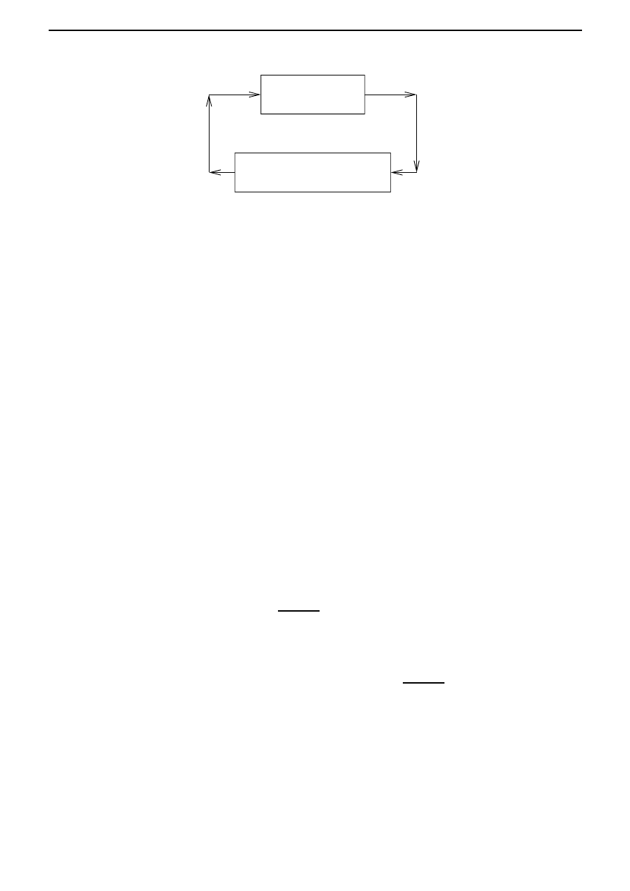
4.4. Constraint on the state at final time. Controllability
43
plant
controller
˙x = Ax + Bu
u(t) =
−R
−1
B
P
∗
(t)x(t)
u
∗
x
∗
Figure 4.1: The closed loop system.
4.4
Constraint on the state at final time. Controllability
In many optimization problems, in addition to minimizing the cost, one may also have to satisfy
a condition for the final state x(t
f
); for instance, one may wish to drive the state to zero. This
brings us naturally to the notion of controllability. For the sake of simplicity, we restrict ourselves
to linear systems:
˙
x(t) = Ax(t) + Bu(t), t
≥ t
i
.
(4.19)
The system (4.19) is said to be controllable if for every pair of vectors x
i
, x
f
in
R
n
, there exists a
t
f
> t
i
and a control u
∈ (C[t
i
, t
f
])
m
such that the solution x of (4.19) with x(t
i
) = x
i
satisfies
x(t
f
) = x
f
. Controllability means that any state can be driven to any other state using an
appropriate control.
Example.
(A controllable system.) Consider the system
˙x(t) = u(t),
so that
A = 0, B = 1.
Then given x
i
, x
f
∈ R, with any t
f
> t
f
, define u
∈ C[t
i
, t
f
] to be the constant function
u(t) =
x
f
− x
i
t
f
− t
i
, t
∈ [t
i
, t
f
].
By the fundamental theorem of calculus,
x(t
f
) = x(t
i
) +
t
f
t
i
˙
x(τ )dτ = x
i
+
t
f
t
i
u(τ )dτ = x
i
+
x
f
− x
i
t
f
− t
i
(t
f
− t
i
) = x
f
.
Note that
rank
B
AB
. . .
A
n−1
B
(n=1)
=
rank
B
= rank
1
= 1 = n,
the dimension of the state space (
R).
Example.
(An uncontrollable system.) Consider the system
˙x
1
(t)
=
x
1
(t) + u(t),
(4.20)
˙x
2
(t)
=
x
2
(t),
(4.21)

44
Chapter 4. Optimal control
so that
A =
1
0
0
1
, B =
1
0
.
The equation (4.21) implies that x
2
(t) = e
t−t
i
x
2
(t
i
), and so if x
2
(t
i
) > 0, then x
2
(t) > 0 for all
t
≥ t
i
. So a final state with the x
2
-component negative is never reachable by any control. Note
that
rank
B
AB
. . .
A
n−1
B
(n=2)
=
rank
B
AB
= rank
1
1
0
0
= 1
= 2 = n,
the dimension of the state space (
R
2
).
The following theorem gives an important characterization of controllability.
Theorem 4.4.1
The system (4.19) is controllable iff rank
B
AB
. . .
A
n−1
B
= n, the
dimension of the state space.
Exercises.
1. For what values of α is the system (4.19) controllable, if
A =
2
1
0
1
, B =
1
α
?
2. (
∗) Let A ∈ R
n×n
and B
∈ R
n×1
. Prove that the system (4.19) is controllable iff every
matrix commuting with A is a polynomial in A.
The following theorem tells us how we can calculate the optimal control when x(t
f
) is specified,
in the case of controllable linear systems.
Theorem 4.4.2
Suppose that the system
˙
x(t) = Ax(t) + Bu(t), t
≥ t
i
is controllable. Let F (
x, u, t) be a continuously differentiable function of each of their arguments.
If u
∗
∈ (C[t
i
, t
f
])
m
is an optimal control for the functional
I
x
i
(u) =
t
f
t
i
F (x(t), u(t), t)dt,
subject to the differential equation
˙x(t) = Ax(t) + Bu(t), t
∈ [t
i
, t
f
], x(t
i
) = x
i
, x(t
f
)
k
= x
f,k
, k
∈ {1, . . . , r},
and if x
∗
denotes the corresponding state, then there exists a p
∗
∈ (C
1
[t
i
, t
f
])
n
such that
∂H
∂
x
(p
∗
(t), x
∗
(t), u
∗
(t), t)
=
− ˙p
∗
(t),
t
∈ [t
i
, t
f
], p
∗
(t
f
)
k
= 0, k
∈ {r + 1, . . . , n}, and
∂H
∂
u
(p
∗
(t), x
∗
(t), u
∗
(t), t)
=
0,
t
∈ [t
i
, t
f
],
where H(
p, x, u, t) = F (x, u, t) + p
(A
x + Bu).

4.4. Constraint on the state at final time. Controllability
45
We will not prove this theorem. Note that for a differential equation to have a unique solution,
there should not be too few or too many initial and final conditions to be satisfied by that solution.
Intuitively, one expects as many conditions as there are differential equations. In Theorem 4.4.2,
we have, in total, 2n differential equations (for x
∗
and p
∗
). We also have the right number of
conditions: n + r for x
∗
, and n
− r for p
∗
.
Exercises.
1. Find a critical control for the functional
I(u) =
1
0
(u(t))
2
dt
subject to ˙x(t) =
−2x(t) + u(t), t ∈ [0, 1], x(0) = 1 and x(1) = 0. Is this control unique?
2. Find a critical control for the functional
I(u) =
T
0
(u(t))
2
dt
subject to ˙x(t) =
−ax(t) + u(t), t ∈ [0, T ], x(0) = x
0
and x(T ) = 0. Find an expression for
the corresponding state. Prove that the critical control can be expressed as a state-feedback
law: u(t) = k(t, T, a)x(t). Find an expression for k(t, T, a).
3. Find a critical control for the functional
I(u) =
T
0
(x
T
− x(t))
2
+ (u(t))
2
dt
subject to ˙x(t) =
−ax(t) + u(t), t ∈ [0, T ], x(0) = x
0
and x(T ) = x
T
.
4. Find a critical control for the functional
I(u) =
1
0
1
2
(u(t))
2
dt
subject to
˙x
1
(t)
=
x
2
(t),
˙x
2
(t)
=
−x
2
(t) + u(t)
t
∈ [0, 1] and
x
1
(0) = 1,
x
2
(0) = 1,
x
1
(1) = 0,
x
2
(1) = 0.
5. (Higher order differential equation constraint.) Find a critical control for the functional
I(u) =
T
0
1
2
(u(t))
2
dt
subject to the second order differential equation
¨
y(t) + y(t) = u(t), t
∈ [0, T ], y(0) = y
0
, ˙
y(0) = v
0
, y(T ) = ˙
y(t) = 0.
Hint: Introduce the state variables
x
1
(t) = y(t), x
2
(t) = ˙y(t).

Chapter 5
Optimality principle and
Bellman’s equation
Bellman and his co-workers pioneered a different approach for solving optimal control problems.
So far we have considered continuous inputs and we have established necessary conditions for the
existence of an optimal control. We now consider a larger class of control inputs, namely piecewise
continuous functions, and in Theorem 5.2.1 we give sufficient conditions for the existence of an
optimal control.
5.1
The optimality principle
The underlying idea of the optimality principle is extremely simple. Roughly speaking, the opti-
mality principle simply says that any part of an optimal trajectory is optimal.
We denote the class of piecewise continuous
R
m
valued functions on [t
i
, t
f
] by
U[t
i
, t
f
].
Theorem 5.1.1 (Optimality principle.)
Let F (
x, u, t) and f(x, u) be continuously differentiable
functions of each of their arguments. Let u
∗
∈ U[t
i
, t
f
] be an optimal control for the functional
I
x
i
(u) =
t
f
t
i
F (x(t), u(t), t)dt,
subject to
˙x(t) = f (x(t), u(t)), t
∈ [t
i
, t
f
], x(t
i
) = x
i
.
(5.1)
Let x
∗
be the corresponding optimal state. If t
m
∈ [t
i
, t
f
), then the restriction of u
∗
to [t
m
, t
f
] is
an optimal control for the functional
˜
I
x
∗
(t
m
)
(u) =
t
f
t
m
F (x(t), u(t), t)dt,
subject to
˙
x(t) = f (x(t), u(t)), t
∈ [t
m
, t
f
], x(t
m
) = x
∗
(t
m
).
(5.2)
Furthermore,
min
u∈U[ti,tf ]
subject to (5.1)
I
x
i
(u) =
t
m
t
i
F (x
∗
(t), u
∗
(t), t)dt +
min
u∈U[tm,tf ]
subject to (5.2)
˜
I
x
∗
(t
m
)
(u).
(5.3)
47

48
Chapter 5. Optimality principle and Bellman’s equation
Proof We have
I
x
∗
(t
m
)
(u
∗
)
=
t
f
t
i
F (x
∗
(t), u
∗
(t), t)dt
=
t
m
t
i
F (x
∗
(t), u
∗
(t), t)dt +
t
f
t
m
F (x
∗
(t), u
∗
(t), t)dt.
(5.4)
From Theorem 1.2.1, it follows that the solution x
1
to
˙x(t) = f
x(t), u
∗
|
[t
m
,t
f
]
(t)
, t
∈ [t
m
, t
f
], x(t
m
) = x
∗
(t
m
),
is simply the restriction of x
∗
to [t
m
, t
f
]. Thus the second term in (5.4) is the cost ˜
I
x
∗
(t
m
)
u
∗
|
[t
m
,t
f
]
(t)
subject to (5.2).
Suppose that there exists a ˜
u
∈ U[t
i
, t
f
] such that
t
f
t
m
F (˜
x(t), ˜
u(t), t)dt = ˜
I
x
∗
(t
m
)
(˜
u) < ˜
I
x
∗
(t
m
)
u
∗
|
[t
m
,t
f
]
(t)
=
t
f
t
m
F (x
∗
(t), u
∗
(t), t)dt.
where ˜
x is the solution to (5.2) corresponding to ˜
u. Define u
∈ U[t
i
, t
f
] by
u(t) =
u
∗
(t)
for t
∈ [t
i
, t
m
),
˜
u(t)
for t
∈ [t
m
, t
f
],
and let x be the corresponding solution to (5.1). From Theorem 1.2.1, it follows that
x
|
[t
i
,t
m
]
= x
∗
|
[t
i
,t
m
]
.
Hence we have
I
x
i
(u)
=
t
f
t
i
F (x(t), u(t), t)dt
=
t
m
t
i
F (x(t), u(t), t)dt +
t
f
t
m
F (x(t), u(t), t)dt
=
t
m
t
i
F (x
∗
(t), u
∗
(t), t)dt +
t
f
t
m
F (˜
x(t), ˜
u(t), t)dt
=
t
m
t
i
F (x
∗
(t), u
∗
(t), t)dt + ˜
I
x
∗
(t
m
)
(˜
u)
<
t
m
t
i
F (x
∗
(t), u
∗
(t), t)dt + ˜
I
x
∗
(t
m
)
u
∗
|
[t
m
,t
f
]
(t)
=
t
m
t
i
F (x
∗
(t), u
∗
(t), t)dt +
t
f
t
m
F (x
∗
(t), u
∗
(t), t)dt
=
I
x
i
(u
∗
),
which contradicts the optimality of u
∗
. This proves that an optimal control for ˜
I
x
∗
(t
m
)
subject
to (5.2) exists and it is given by the restriction of u
∗
to [t
m
, t
f
]. From (5.4), it follows that (5.3)
holds.
Note that we have shown that
min
u∈U[tm,tf ]
subject to (5.2)
˜
I
x
∗
(t
m
)
(u) = ˜
I
x
∗
(t
m
)
u
∗
|
[t
m
,t
f
]
(t)
.
So the theorem above says that if you are on an optimal trajectory, then the best thing you can
do is to stay on that trajectory. See Figure 5.1.
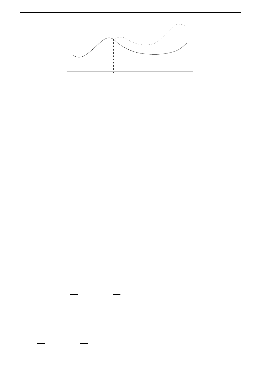
5.2. Bellman’s equation
49
t
i
t
m
t
f
x
i
x
∗
(t
m
)
u
∗
|
[t
i
,t
m
]
˜
u
u
∗
|
[t
m
,t
f
]
Figure 5.1: Optimality principle.
5.2
Bellman’s equation
In this section we will prove Theorem 5.2.1 below, which gives a sufficient condition for the ex-
istence of an optimal control in terms of the existence of an appropriate solution to Bellman’s
equation (5.6). However, we first provide a heuristic argument that leads one to Bellman’s equa-
tion: we do not start by asking when the optimal control problem has a solution, but rather
we begin by assuming that the optimal control problem is solvable and study the so-called value
function, which will lead us to Bellman’s equation.
Let t
m
∈ [t
i
, t
f
). Define the value function V :
R
n
× [t
i
, t
f
]
→ R by
V (x
m
, t
m
) =
min
u∈U[t
m
,t
f
]
t
f
t
m
F (x(t), u(t), t)dt,
(5.5)
where x(
·) is the unique solution to
˙x(t) = f (x(t), u(t)), t
∈ [t
m
, t
f
], x(t
m
) = x
m
.
With this notation, in Theorem 5.1.1, we have shown that
V (x
∗
(t
m
), t
m
) =
min
u∈U[t
m
,t
f
]
t
f
t
m
F (x(t), u(t), t)dt =
t
f
t
m
F (x
∗
(t), u
∗
(t), t)dt.
Consequently
V (x
∗
(t
m
+ ), t
m
+ )
− V (x
∗
(t
m
), t
m
) =
−
t
m
+
t
m
F (x
∗
(t), u
∗
(t), t)dt.
It is tempting to divide by on both sides and let tend to 0. Formally, the left hand side would
become
∂V
∂
t
(x
∗
(t
m
), t
m
) +
∂V
∂
x
(x
∗
(t
m
), t
m
)f (x
∗
(t
m
), u
∗
(t
m
)),
while the right hand side would become
−F (x
∗
(t
m
), u
∗
(t
m
), t
m
).
Thus we would obtain the equation
∂V
∂
t
(x
∗
(t
m
), t
m
) +
∂V
∂
x
(x
∗
(t
m
), t
m
)f (x
∗
(t
m
), u
∗
(t
m
)) + F (x
∗
(t
m
), u
∗
(t
m
), t
m
) = 0.
This motivates the following result.

50
Chapter 5. Optimality principle and Bellman’s equation
Theorem 5.2.1
Let F (
x, u, t) and f(x, u) be continuously differentiable functions of each of their
arguments. Suppose that there exists a function W :
R
n
× [t
i
, t
f
]
→ R such that:
1. W is continuous on
R
n
× [t
i
, t
f
].
2. W is continuously differentiable in
R
n
× (t
i
, t
f
).
3. W satisfies Bellman’s equation
∂W
∂
t
(x, t) + min
u∈R
m
∂W
∂
x
(x, t)f (x, u) + F (x, u, t)
= 0, (x, t)
∈ R
n
× (t
i
, t
f
).
(5.6)
4. W (x, t
f
) = 0 for all x
∈ R
n
.
Then the following implications hold:
1. If t
m
∈ [t
i
, t
f
) and u
∈ U[t
m
, t
f
], then
t
f
t
m
F (x(t), u(t), t)dt
≥ W (x
m
, t
m
),
where x is the unique solution to ˙
x(t) = f (x(t), u(t)), x(t
m
) = x
m
, t
∈ [t
m
, t
f
].
2. If there exists a function υ :
R
n
× [t
i
, t
f
]
→ R
m
such that:
(a) For all (x, t)
∈ R
n
× (t
i
, t
f
),
∂W
∂
x
(x, t)f (x, υ(x, t)) + F (x, υ(x, t), t) = min
u∈R
m
∂W
∂
x
(x, t)f (x, u) + F (x, u, t)
.
(b) The equation
˙
x(t) = f (x(t), υ(x(t), t)), t
∈ [t
i
, t
f
], x(t
i
) = x
i
,
has a solution x
∗
.
(c) u
∗
defined by u
∗
(t) = υ(x
∗
(t), t), t
∈ [t
i
, t
f
] is an element in
U[t
i
, t
f
].
Then u
∗
is an optimal control for the cost functional I
x
i
defined by
I
x
i
(u) =
t
f
t
i
F (x(t), u(t), t)dt,
where x is the unique solution to ˙x(t) = f (x(t), u(t)), t
∈ [t
i
, t
f
], x(t
i
) = x
i
, and furthermore,
I
x
i
(u
∗
) =
t
f
t
i
F (x
∗
(t), u
∗
(t), t)dt = W (x
i
, t
i
).
(5.7)
3. Let υ be the function from part 2. If for every t
m
∈ [t
i
, t
f
) and every x
m
∈ R
n
, the equation
˙x(t) = f (x(t), υ(x(t), t)), t
∈ [t
m
, t
f
], x(t
m
) = x
m
,
has a solution, then W is the value function V defined in (5.5).
5.2. Bellman’s equation
51
Proof
1. We have
t
f
t
m
F (x(t), u(t), t)dt
=
t
f
t
m
∂W
∂
x
(x(t), t)f (x(t), u(t)) + F (x(t), u(t), t)
dt
−
t
f
t
m
∂W
∂
x
(x(t), t)f (x(t), u(t))dt
≥
t
f
t
m
min
u∈R
m
∂W
∂
x
(x(t), t)f (x(t), u) + F (x(t), u, t)
dt
−
t
f
t
m
∂W
∂
x
(x(t), t)f (x(t), u(t))dt
=
t
f
t
m
−
∂W
∂
t
(x(t), t)
−
∂W
∂
x
(x(t), t)f (x(t), u(t))
dt
=
−
t
f
t
m
d
dt
W (x(
·), ·)
(t)dt
=
−W (x(t
f
), t
f
) + W (x(t
m
), t
m
)
=
W (x
m
, t
m
).
2. Let x
∗
be a solution of ˙x(t) = f (x(t), υ(x(t), t)), t
∈ [t
i
, t
f
], x(t
i
) = x
i
. Then we proceed as in
part 1:
t
f
t
i
F (x
∗
(t), u
∗
(t), t)dt
=
t
f
t
i
∂W
∂
x
(x
∗
(t), t)f (x
∗
(t), υ(x
∗
(t), t)) + F (x
∗
(t), υ(x
∗
(t), t), t)
dt
−
t
f
t
i
∂W
∂
x
(x
∗
(t), t)f (x
∗
(t), υ(x
∗
(t), t))dt
=
t
f
t
i
min
u∈R
m
∂W
∂
x
(x
∗
(t), t)f (x
∗
(t), u) + F (x
∗
(t), u, t)
dt
−
t
f
t
i
∂W
∂
x
(x
∗
(t), t)f (x
∗
(t), υ(x
∗
(t), t))dt
=
t
f
t
i
−
∂W
∂
t
(x
∗
(t), t)
−
∂W
∂
x
(x
∗
(t), t)f (x
∗
(t), υ(x
∗
(t), t))
dt
=
−
t
f
t
i
d
dt
W (x
∗
(
·), ·)
(t)dt
=
W (x
i
, t
i
).
But from part 1 (with t
m
= t
i
), we know that if u
∈ U[t
i
, t
f
], then
I
x
i
(u) =
t
f
t
i
F (x(t), u(t), t)dt
≥ W (x
i
, t
i
).
This shows that u
∗
(
·) = υ(x
∗
(
·), ·) is an optimal control and (5.7) holds.
3. We simply repeat the argument from part 2 for the time interval [t
m
, t
f
]. This yields
V (x, t
m
) =
min
u∈U[t
m
,t
f
]
t
f
t
m
F (x(t), u(t), t)dt = W (x, t
m
).

52
Chapter 5. Optimality principle and Bellman’s equation
In the following example, we show how Theorem 5.2.1 can be used to calculate an optimal
control.
Example. Consider the following linear system with state space
R:
˙
x(t) = u(t), t
∈ [0, 1], x(0) = x
0
,
with cost criterion
I
x
0
(u) =
1
0
(x(t))
2
+ (u(t))
2
dt.
For this system, Bellman’s equation is given by
∂W
∂
t
(x, t) + min
u∈R
∂W
∂
x
(x, t)u + x
2
+ u
2
= 0, (x, t)
∈ R × (0, 1), W (x, 1) = 0.
It is easy to see that the minimum in the above is assumed for
u = υ(x, t) =
−
1
2
∂W
∂
x
(x, t).
Thus we obtain
∂W
∂
t
(x, t) + x
2
−
1
4
∂W
∂
x
(x, t)
2
= 0, (x, t)
∈ R × (0, 1), W (x, 1) = 0.
This is a nonlinear partial differential equation. It is easy to see that if (x
∗
, u
∗
) is an optimal
trajectory with initial state x
0
, then for every λ
∈ R, (λx
∗
, λu
∗
) is an optimal trajectory with
respect to the initial state λx
0
. Therefore the value function is quadratic in x: W (λx, t) =
λ
2
W (x, t). In particular,
W (x, t) = x
2
W (1, t) = x
2
p
∗
(t),
where p
∗
(t) := W (1, t). Consequently,
x
2
˙
p
∗
(t) + x
2
−
1
4
(2x)
2
(p
∗
(t))
2
= 0, (x, t)
∈ R × (0, 1), p
∗
(1) = 0.
Dividing by x
2
, we obtain the Riccati equation
˙
p
∗
(t) = (p
∗
(t))
2
− 1, t ∈ (0, 1), p
∗
(1) = 0.
This has the solution
p
∗
(t) =
e
−t+1
− e
t−1
e
−t+1
+ e
t−1
.
(See the exercise on page 3.) Thus
W (x, t) = x
2
e
−t+1
− e
t−1
e
−t+1
+ e
t−1
.
Also the linear time varying differential equation
˙
x(t) = υ(x(t), t) =
−x(t)p
∗
(t), t
∈ [0, 1], x(0) = x
0
has the solution
x
∗
(t) = x
0
e
−
R
t
0
p
∗
(τ)dτ
.
(5.8)
We note that all the conditions from Theorem 5.2.1 are satisfied, so the optimization problem is
solvable. The optimal input is given by
u
∗
(t) = υ(x
∗
(t), t) =
−x
∗
(t)p
∗
(t),

5.2. Bellman’s equation
53
where x
∗
is the optimal state given by (5.8). Note that the optimal control is given in the form of
a (time-varying) state feedback. The value function is given by V (x, t) = x
2
p
∗
(t).
Exercise.
Its good to keep in mind that not every optimal control problem is solvable. Prove that for
the following problem, there is no minimizing input u
∈ U[t
i
, t
f
]:
˙x(t) = u(t), t
∈ [0, 1], x(0) = 1,
with the cost function I
x
0
(u) =
1
0
(x(t))
2
dt.

Bibliography
[1] R.W. Brockett. Finite Dimensional Linear Systems. John Wiley, 1970.
[2] D.N. Burghes and A. Graham. Introduction to Control Theory, Including Optimal Control.
John Wiley, 1980.
[3] I.M. Gelfand and S.V. Fomin. Calculus of Variations. Dover, 1963.
[4] H.J. Sussmann and J.C. Willems. 300 years of optimal control: from the brachystochrone
problem to the maximum principle. IEEE Control Systems, 17:32–44, 1997.
[5] J.L. Troutman. Variational Calculus and Optimal Control: Optimization with Elementary
Convexity. 2nd Edition, Springer, 1996.
[6] R. Weinstock. Calculus of Variations with applications to physics and engineering. Dover,
1974.
[7] H.J. Zwart. Optimal Control Theory. Rijksuniversiteit Groningen, 1997.
55

Index
C[t
i
, t
f
], 19
C
1
[t
i
, t
f
], 19
continuous linear functional, 22
adjoint differential equation, 38
admissible functions, 21
affine linear map, 21
arc length, 21
arc length, 16
Bellman’s equation, 50
brachistochrone problem, 16
calculus of variations, 15
catenary, 29
Cauchy’s problem, 26
closed loop system, 43
co-state, 38
commuting matrices, 6
conservation of energy, 16
constrained optimization problem, 37
continuous functional, 20
control, 1
control system, 2
control theory, 1
controllability, 43
critical control, 38
critical curve, 27
cycloid, 28
dense set, 6
diagonalizable matrix, 6
discount rate, 10
distance, 19
economic growth, 9
economic growth, 14, 39
Euler, 17
Euler-Lagrange equation, 24, 31
exploited population, 11
Frech´
et derivative, 22
free boundary conditions, 31
function spaces, 18
functional, 12
fundamental theorem of calculus, 43
Hamiltonian, 38
Hamiltonian mechanics, 38
Hamiltonian differential system, 38
input, 2
Johann Bernoulli, 16
kernel, 19
Lagrange multiplier, 38
Lagrange multiplier theorem, 37
length of a curve, 12
linear control system, 2
linear functional, 18
linear quadratic control problem, 41
linear space, 18
linear span, 19
linear system, 41
Lipschitz condition, 2
local extremum, 23
LQ problem, 41
method of finite differences, 17
metric space, 19
mixed boundary conditions, 32
norm, 19
normed linear space, 19
optimal control, 13
optimal control theory, 4
optimal state, 13
optimal trajectory, 13
optimality principle, 47
path independence, 13
piecewise continuous, 2
Pontryagin minimum principle, 39
present value, 11
production function, 9
rate of depreciation, 10
rectifiable curve, 12
57

58
Index
relative stationarity condition, 37
Riccati equation, 3, 41, 52
state, 2
state equation, 2
state feedback, 53
state-feedback, 42, 45
static state-feedback, 39
system, 1
Taylor’s theorem, 25
transversality conditions, 31
triangle inequality, 19
underdetermined differential equation, 1
utility function, 10
value function, 49
vector space, 18
vector-valued function, 4
Verhulst model, 11
welfare integral, 10
zero element, 18

Mock examination
MA305
Control Theory
(Half Unit)
Suitable for all candidates
Instructions to candidates
Time allowed: 2 hours
This examination paper contains 6 questions. You may attempt as many questions as you wish,
but only your best 4 questions will count towards the final mark. All questions carry equal
numbers of marks.
Please write your answers in dark ink (preferably black or blue) only.
Calculators are not allowed in this exam.
You are supplied with: Answer Booklet
c
LSE 2004 / MA305 Mock Examination Question Paper
Page 1 of 4

1
(a) Let X be a linear space over
R. Give the definition of a norm on X.
(b) If I : X
→ R is a functional on a normed linear space X, when is I said to be contin-
uous at x
∗
∈ X?
(c) Is the linear functional I : C[0, 1]
→ R defined by
I(x) =
Z
1
0
x(t)dt for x
∈ C[0,1],
continuous at 0? Here the linear space C[0, 1] is equipped with the usual norm
kxk = sup
t
∈[0,1]
|x(t)|.
2
(a) Regarding the left hand side of the obvious inequality
Z
t
f
t
i
(x
1
(t) + rx
2
(t))
2
dt
0
as a quadratic function of r, prove the Cauchy-Schwarz inequality:
Z
t
f
t
i
(x
1
(t))
2
dt
Z
t
f
t
i
(x
2
(t))
2
dt
Z
t
f
t
i
x
1
(t)x
2
(t)dt
2
for all x
1
, x
2
∈ C[t
i
, t
f
].
H
INT
: The minimum value of the quadratic function Q(r) = Ar
2
+ Br + C with
A > 0 is given by
4AC
−B
2
4A
.
(b) Consider the linear functional I defined by
I(x) =
Z
1
0
e
−2t
d
dt
x(t)
2
dt
for x
∈ C
1
[0, 1] with x(0) = 0 and x(1) = 1. Using the result from part (a), show that
I(x)
2
e
2
1
.
H
INT
: Use the Cauchy-Schwarz inequality with x
1
(t) = e
2t
and x
2
= e
−2t d
dt
x(t).
(c) Using the Euler-Lagrange equation, find a critical curve x
∗
for I, and find I(x
∗
).
Using part (b) show that x
∗
indeed minimizes the functional I.
3
Consider the functional I given by
I(x) =
Z
2
0
"
1
2
d
dt
x(t)
2
+ x(t)
d
dt
x(t) +
d
dt
x(t) + x(t)
#
dt
defined for all x
∈ C
1
[0, 2].
(a) Write the Euler-Lagrange equation for this problem.
c
LSE 2004 / MA305 Mock Examination Question Paper
Page 2 of 4

(b) Write the transversality conditions at the endpoints t = 0 and t = 2.
(c) Determine the solution of the Euler-Lagrange equation found in part (a) that satisfies
the transversality conditions from part (b).
4
Consider the functional I : C[0, 1]
→ R defined by
I(u) =
Z
1
0
[3(x(t))
2
+ (u(t))
2
]dt
(1)
where x denotes the unique solution to
d
dt
x(t) =
x(t) + u(t), t
∈ [0,1], x(0) = 1.
(2)
(a) Using the Hamiltonian method, write down the equations that govern an optimal
control for (1) subject to (2).
(b) Find an equation that describes the evolution of the state x
∗
and the co-state p
∗
and
specify the boundary conditions x
∗
(0) and p
∗
(1).
(c) Solve the equations from part (b) and determine a critical control.
5
(a) Consider the controllable linear system
d
dt
x(t) = Ax(t) + Bu(t), t
t
i
,
(3)
where A
∈ R
n
×n
and B
∈ R
n
×m
. Suppose that Q = Q
>
∈ R
n
be a positive semidefinite
matrix and let R = R
>
∈ R
m
be a positive definite matrix. Let I : (C[t
i
, t
f
])
m
→ R
defined by
I(u) =
Z
t
f
t
i
1
2
h
x(t)
>
Qx(t) + u(t)
>
Ru(t)
i
dt,
(4)
where x is the solution to (3) on the time interval [t
i
, t
f
] with x(t
i
) = x
i
∈ R
n
and
x(t
f
) = x
f
∈ R
n
. Using the Hamiltonian theorem on optimal control, write down the
differential equations for the optimal state x
∗
and the co-state p
∗
for I given by (4)
subject to (3).
(b) Give a necessary and sufficient condition for controllability of the system (3) in
terms of A and B.
(c) Show that if the system described by (3) is controllable, then for every
λ
that is an
eigenvalue of A
>
with eigenvector v, there holds that B
>
v
6= 0.
6
Consider the cost functional I : C[0, 1]
→ R defined by
I(u) =
Z
1
0
[3(x(t))
2
+ (u(t))
2
]dt
(5)
where x denotes the unique solution to
d
dt
x(t) =
x(t) + u(t), t
∈ [0,1], x(0) = 1.
(6)
c
LSE 2004 / MA305 Mock Examination Question Paper
Page 3 of 4

(a) Write Bellman’s equation associated with the above functional.
(b) Assuming that the solution W to Bellman’s equation in part (a) is quadratic in x:
W (x, t) = x
2
W (1, t), find a solution W to Bellman’s equation.
(c) Find the optimal state x
∗
and the optimal control u
∗
for I given by (5) subject to (6).
c
LSE 2004 / MA305 Mock Examination Question Paper
Page 4 of 4
Document Outline
- Title
- Preface
- Course description
- Contents
- 1 Introduction
- 2 The optimal control problem
- 3 Calculus of variations
- 4 Optimal control
- 5 Optimality principle and Bellman’s equation
- Bibliography
- Index
- 2004 Mock examination
Wyszukiwarka
Podobne podstrony:
Optimal Control of Three Phase PWM Inverter for UPS Systems
Polymer Processing With Supercritical Fluids V Goodship, E Ogur (Rapra, 2004) Ww
Popper Two Autonomous Axiom Systems for the Calculus of Probabilities
Summary of the Gun Control?bate
Development of wind turbine control algorithms for industrial use
Implementation of budget (EAGGF Guidance Section) (2004)
CALCULATION OF REQUIRED INSULATION 3, BHP, ROSIEK - Mikroklimat, Mikroklimat
Comparison of cartesian vector control and polar
Polymer Processing With Supercritical Fluids V Goodship, E Ogur (Rapra, 2004) Ww
Majewski, Marek; Bors, Dorota On the existence of an optimal solution of the Mayer problem governed
Vol 2 Ch 02 Differential Calculus of Vector Fields
Simulation of a PMSM Motor Control System
Elementary Number Theory Notes D Santos (2004) WW
Meta Math The Quest for Omega G Chaitin (2004) WW
Quick Study Chart Circulatory System (BarCharts Inc, 2004) WW
Baumann Destabilization of velocity feedback controllers with stroke limited inertial actuators
NASA CR 180678 Calculation of Aerodynamic Characteristics at High Angles of Attack for Airplane Conf
więcej podobnych podstron