The Impact of Countermeasure Spreading on the Prevalence of Computer Viruses

Li-Chiou Chen

[e-mail]

Department of Engineering and Public Policy

Carnegie Mellon University

Kathleen M. Carley

[e-mail]

Institute for Software Research International

Department of Engineering and Public Policy

Carnegie Mellon University

The Impact of Countermeasure Spreading on the Prevalence of Computer Viruses

Abstract

How can virus countermeasures such as software patches or warnings be disseminated and

installed more efficiently than they are currently so that fewer organizations will suffer virus

infection problems? The relative effectiveness of four anti-virus strategies is examined formally

using simulations. One of these strategies is the countermeasure spreading strategy (CMS). CMS

is based on the idea that computer viruses and countermeasures spread through two separate

complex networks -- the virus-spreading network and the countermeasure-spreading network, in

which a countermeasure acts as a competing species against the computer virus. We find

evidence to support the adoption of CMS. CMS is as, or more, effective than other strategies.

The proposed CMS reduces the prevalence of computer viruses significantly when the

countermeasure-spreading network has properties that favor countermeasures over viruses, or

when the countermeasure-spreading rate is higher than the virus-spreading rate. Another

advantage is that CMS can be flexibly adapted to different uncertainties in the real world,

enabling it to be “tuned” to a greater variety of situations than other strategies.

— 1 —

The Impact of Countermeasure Spreading on the Prevalence of Computer Viruses

I. INTRODUCTION

Computer virus

1

infections have imposed significant financial losses and loss of productivity to

organizations even though most organizations have installed anti-virus software. The 2002

CSI/FBI Survey [8] estimates that the average annual loss due to virus infections is about 283

thousand dollars per organization based on 223 samples, in which 90% of them have installed

anti-virus software. The 2001 ICSA Computer Virus Prevalence Survey [13] reports that virus

infections have caused server down time, loss of productivity and loss of data for organizations,

in which 92% of them have installed anti-virus software to cover about 90% of their computers.

These evidences show that installing anti-virus software alone cannot solve the virus prevalence

problem effectively unless appropriate anti-virus strategy is taken. Vulnerable computers can still

be infected by new variants of old viruses that exploit the same software vulnerability if virus

countermeasures, such as software patches or new virus definition files, have not been installed

on these computers. How can virus countermeasures be disseminated and installed more

efficiently than they are currently so that fewer organizations will suffer virus infection

problems?

In this paper, we investigate the relative effectiveness of several anti-virus strategies using

computer simulation. A traditional approach to study viruses is to use the Susceptible-Infected-

Removed (SIR) model. SIR is widely used to study the spread of epidemics in human populations

[1][2][10]. The problem with the SIR model is that it only describes the state changes of

populations and cannot explain variations in the underlying networks. However, previous studies

1

A computer virus is a segment of program code that will copy its code into one or more larger “host” programs when it is

activated. A worm is a program that can run independently and travel from machine to machine across network connections [7][23].
In this paper, the term computer virus will refer to both computers viruses and worms since most malicious programs today can be
propagated themselves in both ways.

— 2 —

[1][18][21] have shown that the spread of epidemics in human populations is dramatically

affected by the topology of the underlying network. The same is true of computer viruses [15].

Three anti-virus strategies have been proposed, which add network consideration to the SIR

model to present the spread of viruses. These three strategies are the random immunization

strategy (RANDOM), the targeted immunization strategy (TARGET) [9][18][21], and the kill-

signal strategy (KS) [14][16]. Both RANDOM and TARGET originated in the study of

immunization of human populations to prevent epidemics [10]. These models do not explain how

countermeasures are disseminated for computer viruses. KS considers how countermeasures

spread but does not consider that the network of spreading countermeasures can be different from

the network of spreading viruses. In addition, KS assumes that countermeasures only spread to

computers that have been infected, and does not consider that decision makers for non-infected

computers may also spread countermeasures. We propose an anti-virus strategy called the

countermeasure spreading strategy (CMS) in which countermeasures are spread through a

separate network. Using computer simulation, CMS will be compared with RANDOM,

TARGET and KS.

We can think of a countermeasure as a competing species that acts to suppress the spread of

computer viruses. Decision makers (representing either people or anti-virus software programs)

who receive the countermeasures will adopt them (e.g. install new software patches) and spread

them at a certain probability. CMS is based on the hypothesis that the spread of computer viruses

and the spread of countermeasures are through two separate complex networks: the virus-

spreading network and the countermeasure-spreading network. The real world representations of

these two networks can be either physical networks (connecting computers/programs) or social

networks (connecting people/groups). For example, computer viruses that spread through email

mailing lists utilize the social network connecting email accounts (representing people/groups).

Countermeasures that automatically spread by anti-virus software programs utilize the physical

— 3 —

network connecting computers that have been installed anti-virus software programs. Whether or

not each of these two networks is a social network or a physical network depends on the

vulnerability/information that the virus/countermeasure utilizes in order to spread.

The rest of the paper is outlined as follows. The next section reviews the theoretical

background of our model, briefs other anti-virus strategies and explains CMS in more detail.

Section III describes the virus spreading model and the simulation tool we have developed.

Section IV presents the results of analyzing empirical virus reporting records. Section V

describes the virtual experiments obtained by running our model on hypothetical networks and

on the network inferred from the analysis in section IV. Section VI discusses the results of the

virtual experiments. Contributions and limitations are then discussed.

II. B

ACKGROUND

The spread of computer viruses is a non-linear dynamic system, which is similar to the spread

of epidemics in human populations [14][21]. The Susceptible-Infected-Removed (SIR) model has

been widely used to model the spread of epidemics, and to study immunization strategies

[1][2][10]. This model

2

categorizes the entire populations into three states: susceptible (S),

infected (I) and removed (R). In this model, some of the susceptible population is infected at a

certain rate through contacts with the infected population. At the same time, some of the infected

population recovers at a certain rate, and will not be infected again. The problem with the SIR

model is that it only describes the state changes of the population over time. There are no explicit

network assumptions in the SIR model. However, implicitly it is assuming that everyone is

connected to everyone. This is assuredly not the case in either human or computer networks.

Moreover, previous studies have shown that the spread of epidemics and the spread of computer

2

In this model,

α

denotes the infection rate of susceptible population and

γ

denotes the recovery rate of infected population.

Changes of populations in the three states over time can be represented mathematically as

I

dt

dR

I

SI

dt

dI

SI

dt

dS

γ

γ

α

α

=

−

=

−

=

,

,

.

— 4 —

viruses are dramatically affected by the topology of the underlying networks

[1][15][17][18][19][20][21]. Thus, assuming that the topology is a fully connected network is

leading the SIR to overestimate the rate at which the epidemic, or in this case, the computer

virus, spreads.

Three anti-virus strategies that add network consideration into the SIR model have been

proposed. These strategies are the random immunization strategy (RANDOM), the targeted

immunization strategy (TARGET) [21], and the kill-signal strategy (KS) [14]. RANDOM

proposes to immunize a certain portion of nodes randomly picked from the network of spreading

viruses so that the virus will not prevail because the immunized nodes cannot be used to spread

viruses from one node to another. TARGET proposes a similar strategy but immunizes nodes that

have high connectivity. Both strategies have been studied for controlling epidemic spreading in

human populations [1] and for controlling computer virus spreading through complex networks

[9][18][21][24]. KS proposes that once virus infection is found in a computer, the computer will

disseminate countermeasures to other infected computers. KS assumes that the adoption of

countermeasures is mandatory, and does not assume countermeasures are spread through a

separate network. In addition, KS assumes that countermeasures only spread to the computers

that have been infected, and does not consider that decision makers for other computers may

spread countermeasures as well. We refer the model proposed in [14] as the KW model.

The countermeasure-spreading strategy (CMS) we propose is based on the hypothesis that

countermeasures against a new computer virus can be spread through a countermeasure-

spreading network. The spread of countermeasures is similar to the spread of computer viruses

but countermeasures act to suppress the spread of computer viruses. You can think of this as

having two viruses spreading at the same time – a good one and a bad one. Factors that influence

the spread of the good over the bad enable the overall system to be less likely to be impacted by

the bad virus. The content of countermeasures depends on the implementation of this strategy. A

— 5 —

common example is spreading email warnings that ask people to be aware of new computer

viruses or new software vulnerabilities. Another example is to create an automatic mechanism

for spreading software patches exploited by new viruses. Users who like to adopt the automatic

mechanism can install a software program on their computers to authenticate and spread the

software patches. A similar mechanism has been implemented in most current anti-virus software

products

3

but these products only allow a server to disseminate countermeasures to other client

computers, which cannot further spread countermeasures.

The paper will focus on investigating the relative effectiveness of CMS so that we can draw

implications for real world implementations. However, the specific implementation details are

beyond the scope of this paper. In the next section, we will explain our model that extends the

SIR model to simulate CMS.

III. M

ODELING THE DYNAMICS OF COMPUTER VIRUS PROPAGATION

This section describes the model of virus spreading and countermeasure spreading, and the

simulation tool to examine CMS. Table A-I in Appendix A lists the notations and meanings of

parameters used in the model. The goal of the model is to generate implications on the anti-virus

strategies of reducing the prevalence of computer viruses. Our approach is to model the computer

virus prevalence problem in the real world at an abstract level that can generate useful policy

conclusions. We are not trying to model the exact real world details.

A. The model of

virus spreading and countermeasure spreading

We define virus-spreading network G

v

as the network for spreading viruses, and

countermeasure-spreading network G

c

as the network for spreading countermeasures. Both G

v

and G

c

are undirected graphs. In the real world, both networks can represent either physical

networks (connecting computers/programs) or social networks (connecting people/groups). The

3

For example, Symantec, McAfee and Sophos all have products to support this functionality.

— 6 —

real world representation of G

v

depends on the vulnerabilities that the virus exploits. For

example, the computer virus that spreads through emails or mailing lists, such as Love Letter,

propagates itself to other email accounts only when email receivers click on the malicious email

attachments. In this case, G

v

is a social network because the virus exploits the

social/organizational connections among people/groups that are built upon email

communications, in which the virus spread from one email account (representing one person or

one group) to another email account. On the contrary, the computer virus that exploits specific

software vulnerabilities, such as Nimda, can propagate itself without user interventions. In this

case, G

v

is a physical network connected by vulnerable computers/programs. Similarly, the real

world representation of G

c

depends on the implementation of anti-virus policies. For example, G

c

is a social network if countermeasures are implemented as email warnings, because the warnings

spread from one email account (representing one person or one group) to another. In contrast, G

c

is a physical network if countermeasures automatically spread through anti-virus programs that

have been installed by system administrators on computers beforehand. In summary, the

differences in these two complex networks in the model are not exactly the differences between a

physical network and a social network. Whether or not G

v

or G

c

is a social network or a physical

network depends on the vulnerability/information that the virus/countermeasure utilizes in order

to spread.

In this paper, we make two simplifying assumptions which facilitate evaluating the

effectiveness of CMS. These assumptions can be relaxed in future applications of our model.

First, we assume that countermeasures have only a positive effect, no negative effect, on the

action of decision makers. For example, a software patch is authenticated that can actually patch

the software vulnerability, but is not another computer virus. Secondly, we assume that each

node in G

v

maps to one node in G

c

. For example, the decision maker that receives a

countermeasure will only apply it on the set of computers in the administrative domain of the

— 7 —

decision maker.

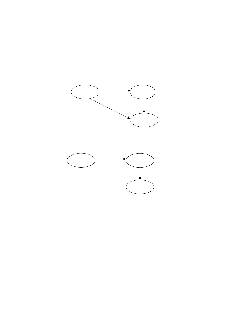
The changes of each node in these two complex networks are described as state machines.

Each node in G

v

changes over time among three states: “susceptible (S)”, “infected (I)”, and

“removed (R)” due to computer virus spreading, as illustrated in the state machine in Fig. 1. In

the meantime, each node in G

c

changes among three states: “unwarned (U)”, “warning (WG)”

and “warned (WD)” due to countermeasure spreading, as illustrated in the state machine in Fig.

2. In each state machine, circles represent states and arrows represent state transition rules. We

label each arrow with the name of the state transition rule and a Roman symbol representing the

probability of change for each node from one state to another state. All probabilities of change

for state transition rules are in range [0,1]. We describe these states and rules in details as

follows.

1) The state machine of spreading computer viruses

Each state in the state machine of spreading computer viruses represents an observable fact

Unwarned

(U)

Warning

(WG)

Propagating

countermeasures (

λ

)

Stopping countermeasures
spreading (

δ

)

Warned

(WD)

Fig. 2. The state machine of spreading countermeasures

Susceptible

(S)

Infected

(I)

Removed

(R)

Patching
computers from
susceptible (

κ

)

Propagating viruses (

α

)

Patching computers
from infected (

γ

+

κ

)

Fig. 1. The state machine of spreading computer viruses

— 8 —

of a node. A state is a Boolean variable in value either “true” or “false”. The state machine is

revised from the SIR model, which includes three states:

1. Susceptible (S): A node has the software vulnerability that the computer virus exploits.

2. Infected (I): A node is infected by the computer virus, which means the node can infect its

neighbors with this virus and the virus has not been removed from the node. For example,

computers that receive a Melissa Virus are in infected “state” only if the users click on the

email attachments and only if the computers can spread this virus.

3. Removed (R): A node that has installed a detection tool that has the functionality to detect

the computer virus, or the node has installed a software patch to eliminate the software

vulnerability that this computer virus exploits.

There are three state transition rules for spreading viruses:

1.

Propagating viruses: A node in the “susceptible” state will change to “infected” state

with the probability

α

only if one of its neighbors is infected, where

α

is the birth rate of

the computer virus.

2.

Patching computers from infected: A node in the “infected” state will change to

“removed” state at the probability

γ

, where

γ

is the die out rate of the computer virus

because decision makers have discovered virus infections and patched the computers. In

addition, if the corresponding node in G

c

is in either the “warning” state or the “warned”

state, the probability of patching is increased from

γ

to

γ

+

κ

.

κ

denotes the countermeasure

adoption rate and represents the probability that decision makers will adopt the

countermeasure. In order to discuss how fast a virus can spread when no countermeasure

is applied, we define the virus-spreading rate

ρ

v

=

γ

α

.

3.

Patching computers from susceptible: A node in the “susceptible state will change to

“recovered” state at the probability

κ

if the corresponding node in G

c

is in either the

— 9 —

“warning” state or the “warned” state. We assume that

κ

for susceptible nodes is the same

as the one for infected nodes. These two adoption rates may be different in the real world

but it does not influence our purpose of investigating the relative effectiveness of CMS.

2) The state machine of spreading countermeasures

Each state in the state machine of spreading countermeasures represents if a decision maker

will adopt and spread countermeasures. A state is a Boolean variable in value either “true” or

“false”. This state machine includes three states:

1. Unwarned (U): The node has not received the countermeasure and the computers

administrated by this node will not be influenced by the countermeasure.

2. Warning (WG): The node has received countermeasures and spreads the countermeasure.

The decision maker will adopt the countermeasure at a certain probability and spread the

countermeasure to its neighbors.

3. Warned (WD): The node has received countermeasures but does not spread the

countermeasure anymore. Nodes at this state will adopt the countermeasure at a certain

probability but does not spread the countermeasure to its neighbors.

There are two state transition rules for spreading countermeasures:

1.

Propagating countermeasures: A node in the “unwarned” state will change to the

“warning” state with the probability

λ

if one of its neighbors is in the “warned” state,

where

λ

is the birth rate of the countermeasure.

2.

Stopping countermeasures spreading: A node in the “warning” state will change to

“warned” state at the probability

δ

, where

δ

is the die out rate of the countermeasure. We

model that a node stops spreading the countermeasure at a certain probability for two

reasons: First, if the countermeasure represents an email warning, people who have

received the emails may not keep propagating the emails all the time. Secondly, if the

countermeasure represents a software patch sent by an automatic mechanism, the die out

— 10 —

rate will prevent the patch spreading from saturating the computer network. In order to

discuss how fast a countermeasure can spread, we define the countermeasure-spreading

rate

ρ

c

=

δ

λ

.

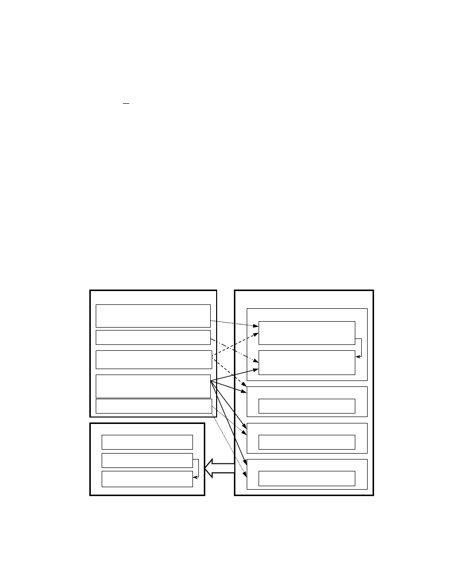
B. The simulation on the prevalence of computer viruses

The simulation is designed to be flexible enough so that it can examine the relative

effectiveness of four different anti-virus strategies on different network topologies using Monte-

Carlo sampling techniques. The four strategies are RANDOM, TARGET, KS, and CMS, as

described in the Section II. These four strategies are based on four different state machines: our

state machine of spreading viruses, our state machine of spreading countermeasures, the state

machines from the KW model, and the state machine from the SIR model. In addition, the

simulation tool is able to import a given network topology, and to simulate the spread of

Input

Countermeasure-spreading

network (G

c

)

Virus-spreading network (G

v

)

Virus-spreading rate (

ρ

v

)

Strategies (State machines)

Countermeasure spreading (CMS)

Kill-signal spreading (KS)

Random immunization (RANDON)

Targeted immunization (TARGET)

Output

Prevalence (P)

Converge time (T)

The SIR model

The KW model

The state machine of

spreading countermeasures

The state machine of

spreading computer viruses

The SIR model

Relative Prevalence (RP)

Countermeasure adoption rate (

κ

)

Percentage of nodes immunized (n)

Countermeasure-spreading rate (

ρ

c

)

Fig. 3. The simulation on the prevalence of computer viruses

— 11 —

computer viruses using this network.

Fig. 3 illustrates the design of the simulation. The inputs include G

c

and

κ

, which are only used

by CMS,

ρ

c

, which is used by CMS and KS, G

v

and

ρ

v

, which are used by all four strategies, and

percentage of immunized nodes (n), which are used by RANDOM and TARGET. Each

simulation stops when the dynamic system is converged to a steady state. In our simulation, the

steady state means that no nodes are in the “infected” state or all nodes have been infected. The

outputs include converge time (T), prevalence (P) and relative prevalence (RP). Converge time

(T) is the time that the system converges, which is the time that the simulation stops. Prevalence

(P) is the number of nodes that have been infected divided by the total number of nodes in the

network. Relative prevalence (RP) is the relative value of P comparing to no anti-virus strategy.

In the next section, we will estimate the empirical values of P and T from The Wild List data.

IV. A

NALYSIS OF VIRUS REPORTING RECORDS

A computer virus propagates itself based on the infection mechanism coded in this virus

program. The virus-spreading network G

v

and the virus-spreading rate

ρ

v

depend on the design of

the infection mechanisms coded in a virus program, and the vulnerability that is exploited by the

computer virus. In this section, we calibrate G

v

and

ρ

v

based on The Wild List

4

(TWL) virus

prevalence records. The data set we analyzed is from January 1996 to September 2002, which

includes 106 reporting sites and 958 computer viruses across 71 reporting

5

time periods. TWL

was originally published in one-month chucks. It reports the name of the viruses that have been

discovered in each reporting site (a site refers to a company or a reporting center) over time but

does not report the number of infected computers in each site. For this reason, this data set is

only enough to investigate the prevalence of compute viruses among organizations but not within

4

The Wild List is available at http://www.thewildlist.com. It is a cooperative listing of viruses reported as being in the wild by

virus information professionals. ICSA, Virus Bulletin and Secure Computing are currently using The Wild List as the basis for virus
testing and certification of anti-virus products [12].

5

From 1996-1998, The Wild List reported the records every two months.

— 12 —

an organization.

A. Prevalence and converge time

We categorize viruses in TWL data set into two types: one-to-one and one-to-many, because

we would like to know if P and T in these two types are different. One-to-one refers to the virus

that is designed to infect one target during one infection process and this infection process is

triggered by a certain user behavior, such as a MS macro virus. One-to-many refers to the virus

that is designed to infect multiple targets during one infection process and the virus itself can

trigger the infection process automatically, such as the Melissa virus [5] or the Love Letter virus

[6]. Table I lists minimum, mean, maximum, and standard deviation of P

6

and T

7

.

Table I: Prevalence and converge time from TWL data set

All

data

One-to-one One-to-many

Number of viruses

958 821

137

Prevalence (P) Minimum

0.02 0.02

0.02

Mean

0.09

0.08

0.14

Maximum

0.60 0.60

0.57

Standard

deviation 0.11

0.10

0.14

Converge time (T) Minimum

1 1

2

Mean

15.9

16.2

15.0

Maximum

71 71

60

Standard

deviation 12.6

13.1

8.5

From this analysis, we have found the following characteristics of computer virus spreading:

1.

On average, one-to-many viruses spread faster than one-to-one viruses since the average P

is higher and the average T is shorter. However, the fastest spreading one-to-one virus can

infect as many sites as one-to-many viruses. In addition, the variations of P between the

two types are similar (standard deviation=0.10 and 0.14 respectively).

6

Prevalence= the number of sites that have reported a virus/ the total number of reporting sites

— 13 —

2.

The standard deviation of T is 12.6 months and the average T is 15.9 months. This result

implies that the variation of T among different viruses is relatively large (more than a

year). By further examining the data set, we found that viruses spread much faster in the

first three months than the rest of their lifetime. In the first three months, one-to-many

viruses have infected average 83% of the sites that are infected when the viruses

converge, and one-to-one viruses have infected average 77% of those.

Since both types of viruses are able to cause P as high as 0.6, it is more meaningful to

examine the effectiveness of CMS based on the fastest spreading virus. We will use P =0.6

(maximum) and T= three months (infect roughly 80% of sites) as base values to calibrate

ρ

v

in

the next section.

ρ

v

calibrated from this data set may be underestimated due to two reasons.

First, TWL data set is an observed virus prevalence records in which it is possible that some

virus infection incidents are not reported because they have not been discovered. Secondly, the

observed prevalence records may be a result of applying some anti-virus strategies. For this

reason, we examine the variation of

ρ

v

in the simulation in the Section VI.

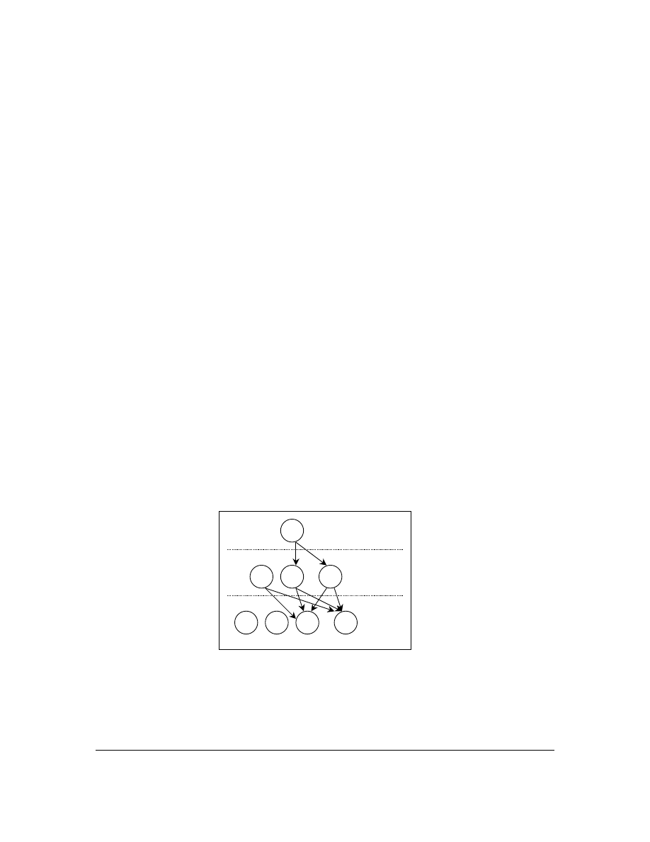
B. The network of computer virus spreading

To order to infer G

v

, we investigate the change of reporting sites over time for each virus. We

coded the reporting records for each virus as a network. The data coding assumes that two

7

Converge time= the last time period that a virus was shown on the list - the first time period that the virus was reported.

A

C

A

E

C

B

D

B

T

1

T

2

T

3

Fig. 4. An example of inferring the virus-spreading network

— 14 —

reporting sites have a link to each other if one site reports a virus during the current time period

and the other site reports the same virus the first time during the next time period. This

assumption implies that the virus is spread from one site to another either directly from this site

or indirectly through another sites during this time period. Fig. 4 shows an example. This

example illustrates that a virus is reported in three continuous reporting periods: T

1

, T

2

, and T

3

.

Site A reported the virus in the time period T

1

, and sites A, B, and C reported the same virus in

the time period T

2

. We assume that a link exists between A and B, and A and C since B and C

were reported in the next time period that A was reported. The same coding assumption is

applied to the next time period until all time periods are included. At the end, we obtain G

v

for

this computer virus. A similar approach to investigate the time evolution of networks has been

used in the social network analysis [3].

By applying the same assumption to each virus, we obtain a set of virus-spreading networks G

={G

k

| k = 1, 2,…, 958}. Each graph in G contains the observable nodes that a virus actually

infects but does not contain the nodes that are susceptible to the virus. G

v

should be larger than

the observable one. For this reason, we calculate G

v

as the conjunction of graphs in G, in which a

link exists only if the link is observed at least in

ϕ

networks in G. In the social network analysis,

this method has been used to find a central graph from a set of networks [22]. We set

ϕ

=2 which

is the largest possible network that has been used by at least two viruses. G

v

calculated from this

method represents the worst possible case of computer virus spreading, which can examine the

lower bound of CMS. We refer G

v

inferred from TWL data set as TWL in the following sections.

V. V

IRTUAL

E

XPERIMENTS

In this section, we describe simulation experiments to evaluate the effectiveness of CMS. For

each experiment, parameters are initialized as specified in the experiment designs in the next

sub-sections. Each experiment is run 10

5

times so that the standard deviations and the mean

— 15 —

values of outputs converge. One starting infected node is randomly selected each run

A. Base

scenario

All parameters in an experiment will be set to a base scenario except for specified in the

experiment designs. The base scenario will be used as a benchmark for anti-virus strategies since

it describes the situation that a virus is spreading but no anti-virus strategy is applied. In the base

scenario, we calibrate

ρ

v

= 0.13 (

ρ

v

=

α

/

γ

where

α

= 0.013 and

γ

= 0.1) in which the average P =

0.6 and the average T = 90 days (3 months) as we estimated in the Section IV.A. All other

parameters are set to zero in the base scenario. TWL network is used in the base scenario.

B. Measures of effectiveness

In order to measure how effective an anti-virus strategy is, we will report the results in P or RP

in the next Section. P is calculated as the average value in 10

5

runs. RP is calculated as the ratio

of P based on one strategy to P without any anti-virus strategy. RP indicates how much

prevalence an anti-virus strategy can reduce relative to the prevalence without any strategy at all.

For example, RP = 0.5 means that the strategy can reduce prevalence to a half of prevalence

without this strategy. Both P and RP are in range [0,1].

C. Designs of virtual experiments

How effective CMS is? We will run 6 sets of virtual experiments to investigate this question.

Table A-II in Appendix B lists the values of parameters in each experiment.

Both Experiment 1 and 2 investigate the effectiveness of CMS based on TWL network, in

which Experiment 1 varies

ρ

v

and

κ

and Experiment 2 varies

ρ

c

and

κ

. Experiment 3 and 4

investigate how network topology influences the effectiveness of CMS by varying either G

v

or

G

c

. In Experiment 3, the networks include TWL network, a scale-free network (SF)

8

, a Small-

World network with reconnecting probability=0 (SM0)

9

, a Small-World network with

8

All scale-free networks are generated based on the algorithm in [4].

9

All Small-World networks are generated based on the algorithm in [26]. SM0 refers to a lattice. SM1 refers to the edges in a

lattice are reconnecting to other nodes with the probability =1.

— 16 —

reconnecting probability=1 (SM1), and a fully connected network (FULL). All SF, SM0, SM1

and FULL networks are the same size as TWL network (106 nodes). In Experiment 5, we

investigate networks with more nodes. An Internet autonomous system network topology

10

(AS)

is used, which has 11,716 nodes. The link distribution of Internet autonomous system network

topology is proportional to several power-law relationships [11], which is different from

topologies in Experiment 3. Three other networks with the same number of nodes are compared

to AS, which include a scale-free network (SF-L), a Small-World network with reconnecting

probability=0 (SM0-L), a Small World network with reconnecting probability=1 (SM1-L), and a

fully connected network (FULL-L). Properties of networks used in Experiment 3 and 4 are listed

in Table A-III in Appendix C. Experiment 5 compares CMS with three other anti-virus strategies,

including RANDOM, TARGET and KS.

VI.

RESULTS OF VIRTUAL EXPERIMENTS

Using results from simulation experiments, this section investigates the relative effectiveness of

CMS by varying

ρ

v

,

ρ

c

,

κ

, G

v

, and G

c

. In addition, the section compares CMS with three other

anti-virus strategies.

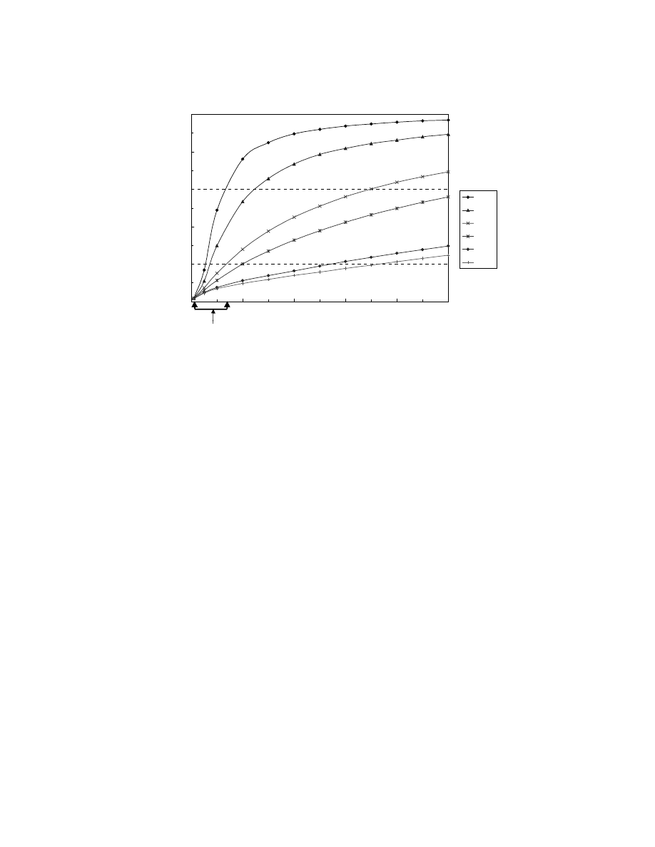
A. The impact of virus-spreading rate

10

Available at “http://moat.nlanr.net/AS/ “, downloaded on August 2001.

— 17 —

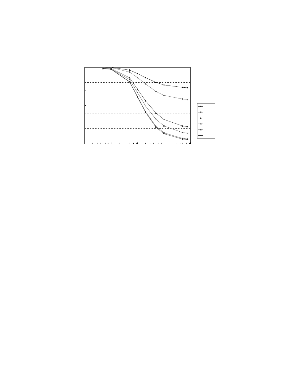
First, we investigate CMS under various

ρ

v

. As in Fig. 5, the results from Experiment 1 show

that CMS reduces prevalence

11

to about one third of its original level (from 0.6 to 0.2) if the

probability that decision makers will adopt countermeasures is 0.05, in which the virus spreads at

the maximum

ρ

v

observed in TWL data set.

To examine viruses that may spread much faster than the observed one, we investigate

ρ

v

that

are higher than the observed maximal value. From Fig. 5, when

ρ

v

is twice of the observed

maximal value and

κ

=0.1, prevalence is reduced to about one third of its original level (from 0.85

to 0.25). When

ρ

v

is ten times of the observed maximal value,

κ

=0.5 is needed for the same

result. These results imply that CMS is only effective when

κ

increases with

ρ

v

. From Fig. 5, we

also found that increasing

κ

from 0.01 to 0.5 reduces prevalence more than increasing

κ

from 0.5

to 1. This result implies that CMS can be effective even though less than 50% of nodes adopt

11

We present the result of experiment 1 in prevalence instead of relative prevalence so that we can show the result for the base

scenario (adoption rate = 0). Later in this section, results will be reported in relative prevalence in order to show the relative change of
prevalence because of anti-virus strategies.

0

0.2

0.4

0.6

0.8

1

0

0.2

0.4

0.6

0.8

1

Virus-spreading rate (

U

v

)

Pr

evalence (P)

0
0.01
0.05
0.1
0.5
1

Counter-
measure
adoption
rate (

κ

)

TWL data set
0.012

≤ρ

v

≤

0.13

Fig. 5. The effectiveness of CMS when virus-spreading rate (

ρ

v

) and countermeasure

adoption rate

(κ)

vary (where

ρ

c

/

ρ

v

=10)

— 18 —

countermeasures once they receive them.

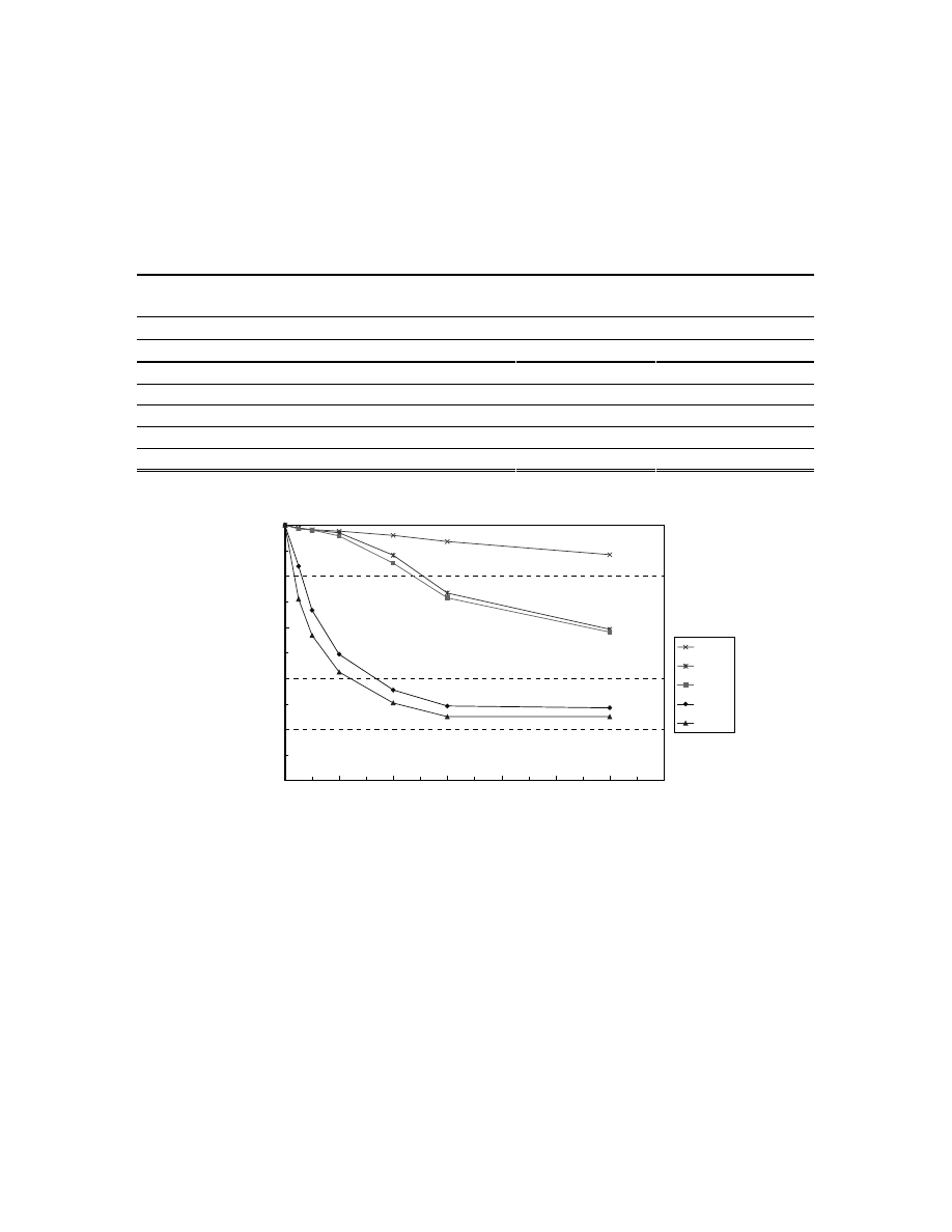
B. The impact of countermeasure-spreading rate

How fast should the countermeasure spread in order to significantly reduce prevalence? The

results from Experiment 2 (Fig. 6) address this question. If the countermeasure spreads as fast as

the computer virus does (

ρ

c

/

ρ

v

= 1), prevalence will be reduced to less than 0.6 of its original

level even though all nodes adopt the countermeasure. However, prevalence is reduced to more

than a half of its original level if

ρ

c

is larger than

ρ

v

(

ρ

c

/

ρ

v

> 1), and if each node has at least 0.05

possibilities to adopt the countermeasure (

κ

≥

0.05). This result implies that, when

ρ

c

is larger

than

ρ

v

, CMS can significantly reduce prevalence even though the probability of decision makers

to adopt countermeasures is low.

C. The impact of network topology

The topology of G

v

may vary from one virus to another. For example, G

v

for a virus spreading

through emails is different from G

v

for a virus spreading through web browsing. Similarly, the

0.0

0.2

0.4

0.6

0.8

1.0

0.01

0.1

1

10

100

Ratio of countermeasure-spreading rate

to virus-spreading rate (

U

c

/

U

v

)

R

e

lative Pr

evalence (R

P)

0.005

0.01

0.05

0.10
0.50

1.00

Counter-
measure
adoption
rate

(κ)

Fig. 6. The effectiveness of CMS when countermeasure-spreading rate

(ρ

c

)

and countermeasure

adoption rate

(κ)

varies

— 19 —

topology of G

c

may vary from one anti-virus policy to another. For example, G

c

for sending email

warnings is different from G

c

for sending software patches by system administrators. The

variation of networks in the real world is the reason why we need to study the impact of network

topology.

Table II: Correlations between properties of countermeasure-spreading networks (G

c

) and

relative prevalence (RP)

The ratio of countermeasure-spreading rate to virus spreading rate (

ρ

c

/

ρ

v

)

0 0.5 1 2 4 6 12

Epidemic

threshold

0 0.65 0.84 0.93 0.94 0.92 0.92

Density

0 -0.98 -0.86 -0.71 -0.58 -0.51 -0.49

Average path length

0

0.24

0.30

0.36

0.47

0.56

0.64

Clustering

coefficient 0 -0.83 -0.82 -0.68 -0.52 -0.42 -0.36

Degree centralization

12

0 -0.75 -0.55 -0.25 -0.18 -0.18 -0.22

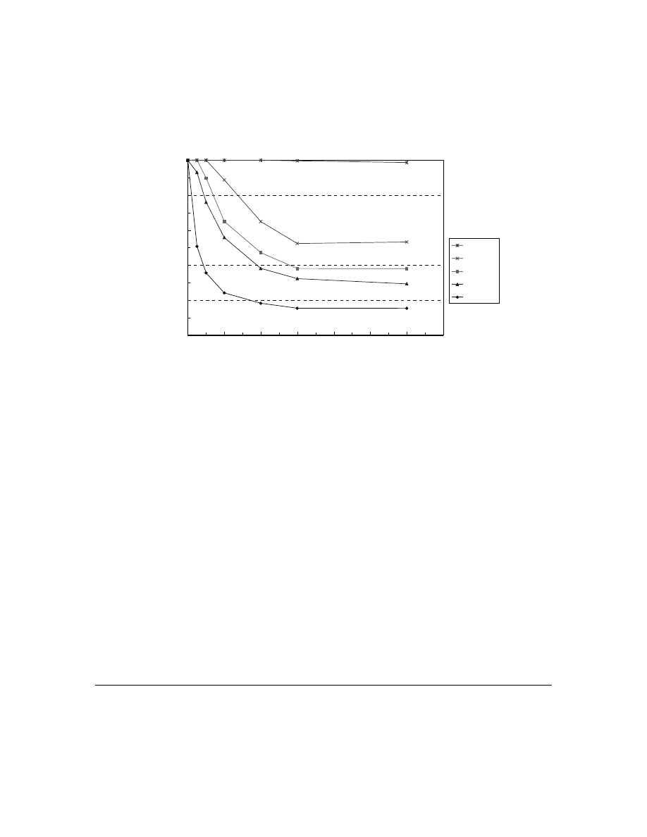
First, we ask how does G

c

influence the effectiveness of CMS? As in both Fig. 7 and Fig. 8, we

find that the effectiveness of CMS varies with G

c

. In order to investigate what properties in a

network actually influence this strategy, we correlate properties of networks to relative

0

0.2

0.4

0.6

0.8

1

0

2

4

6

8

10

12

14

Ratio of countermeasure-spreading rate

to virus-spreading rate (

U

c

/

U

v

)

R

e

lative pr

evalence (R

P)

SM0
SM1
SF
TWL
FULL

Counter-
measure
spreading
network
(G

c

)

Fig. 7. The effectiveness of CMS when the topology of countermeasure-spreading network

(G

c

) varies (virus-spreading network G

v

is fixed to TWL)

— 20 —

prevalence generated in Experiment 3 and 4. As in Table II, we find that the correlation varies

with both

ρ

c

and the properties of networks.

Among the properties we calculated, epidemic threshold has the highest positive correlation to

relative prevalence when

ρ

c

is larger than

ρ

v

(

ρ

c

/

ρ

v

>1). Epidemic threshold is defined as the

minimal epidemic spreading rate that an epidemic can prevail [1]. In a complex network,

epidemic threshold varies with the edge distribution of networks

13

[19]. Applying this property on

countermeasure spreading, we find that the countermeasure-spreading network with a lower

epidemic threshold is more effective to reduce the prevalence of computer viruses than the ones

with higher epidemic thresholds. For example, Fig. 7 illustrates this result where the order of

epidemic thresholds is SM0>SM1>SF>TWL>FULL. In general, this result confirms that the

prevalence of an epidemic increases when the epidemic threshold of the network decreases.

12

Degree centralization can be used as an index only if it is larger than 1 because all graphs that have the same number of edges

per node have degree centralization = 1. For example, both a fully connected network and a lattice network have degree centralization
=1. For this reason, this index cannot distinguish edge distribution among nodes well when it is equal to 1.

0

0.2

0.4

0.6

0.8

1

0

2

4

6

8

10

12

14

Ratio of countermeasure-spreading rate

to virus-spreading rate (

U

c

/

U

v

)

Rel

a

ti

ve pr

eval

ence (

R

P)

SM0-L
SM1-L
SF-L
AS
FULL-L

Counter-
measure
spreading
network
(G

c

)

Fig. 8. The effectiveness of CMS when the topology of countermeasure-spreading network (G

c

)

varies (virus-spreading network G

v

is fixed to AS)

— 21 —

In addition, density

14

has a negative correlation with relative prevalence. This result implies

that our strategy is more effective if the connectivity of G

c

is larger. This confirms that the

prevalence of epidemics (applied to countermeasures in this case) increases with the connectivity

of the network for spreading epidemics. Moreover, the effectiveness of CMS increases with

clustering coefficient

15

(negatively correlated to relative prevalence), and decreases with average

path length (positively correlated to relative prevalence). This result implies that the prevalence

of epidemics increases when the cliquishness of the network for epidemic spreading increases,

and decreases when the average path length of the network increases. This result confirms the

finding in [26] about epidemic spreading on a network with the Small-World property. Finally,

we found that the effectiveness of CMS increases when the degree centralization

16

[25] of a

network increases. However, the correlation is smaller comparing to other measures.

In Experiment 3 and 4, we also investigate the effectiveness of CMS when G

v

varies. We find

that the influence of network topology is two folds. If G

c

and G

v

have the same property, this

property influences the spread of viruses as the same way as the spread of countermeasures. In

this case, the effectiveness of CMS increases when the ratio of

ρ

c

to

ρ

v

increases, as in Fig. 7

(both networks=TWL) and Fig. 8 (both networks=AS). However, if the properties of G

c

are

different from those of G

v

, the effectiveness depends on the ratio between the properties of these

two networks. For example, in Fig. 8, relative prevalence for different topologies is higher when

the epidemic threshold of G

c

(SM0-L, SM1-L and SF-L) is larger than the epidemic threshold of

G

v

(AS). Hence, to suppress the spread of computer viruses, G

c

needs to have the properties that

will spread the countermeasures faster than the viruses.

13

When an epidemic spreads on a complex network, the epidemic threshold can be estimated by

>

<

>

<

=

2

e

e

threshold

ρ

where

<e> denotes the average number of edges and <e

2

> denotes the average square of edges [19].

14

Density measures the connectivity of a network, which is defined as the number of edges of a network divided by the largest

possible number of edges of this network [25].

15

Clustering coefficient measures the cliquishness of a network. Node clustering coefficient is defined as the connectivity of the

neighbors of a node. Clustering coefficient is the average of node clustering coefficients in a network [26].

— 22 —

D. Large

networks

Is CMS applicable to larger networks? Experiment 4 confirms that CMS has the same property

in larger networks as in small networks. In Experiment 4, an Internet autonomous system

network topology (AS) is compared with other hypothetical network topologies that have the

same number of nodes (11,716 nodes) and the same connectivity. Assume that in the future AS is

used for spreading viruses, the effectiveness of CMS (FULL-L>AS>SF-L>SM1-L>SM0-L) is

correlated to the properties of G

c

, as in Table II and as in Fig. 8.

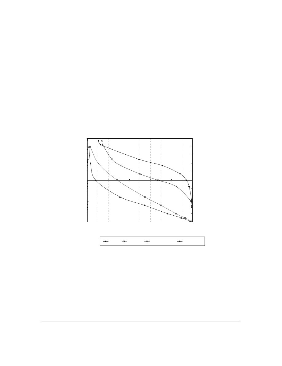
E. Comparison of different anti-virus strategies

Comparing to other anti-virus strategies, how effective CMS is? Experiment 5 (Fig. 9) shows

how relative prevalence varies if a different anti-virus strategy is applied. For example, to reduce

prevalence to a half of its original level (RP=0.5), KS requires

ρ

c

is 10 times of

ρ

v

; CMS requires

ρ

c

is twice of

ρ

v

and

κ

=0.1; RANDOM requires 35% of the nodes are immunized and TARGET

16

Degree centralization measures the differences of the connectivity among nodes, which takes the average of the difference of

individual node connectivity and the average node connectivity [25].

0.01

0.1

1

10

100

0.0

0.2

0.4

0.6

0.8

1.0

Relative prevalence (RP)

Ratio of countermeasure-

spreading rat

e

to

virus-

spreading rat

e

(

U

c

/

U

v

)

fo

r KS

and CM

S

0%

20%

40%

60%

80%

100%

Per

centage of nodes immunized

(n

)

fo

r RANDOM

and TARGE

T

KS

CMS

RANDOM

TARGET

Anti-Virus Strategy

Fig. 9. The effectiveness of CMS comparing to other strategies (the vertical axis of KS and

CMS is on the left, and the vertical axis of RANDOM and TARGET is on the right)

— 23 —

requires 25% of the nodes are immunized.

Each of these four strategies has its strength and weakness. Both RANDOM and TARGET

require a few nodes immunized before a virus infect them. In the real world, to immunize a node

is possible because patching software vulnerabilities in computers or setting a virus filter at the

email server of an organizational network can be regarded as a form of immunization. In theory,

TARGET is more effective because it can reduce prevalence to the same level as RANDOM

does by immunizing fewer nodes [21]. However, it is hard to determine which nodes have high

connectivity in the computer virus problem. In this aspect, RANDOM is more applicable to the

real problem than TARGET.

Both KS and CMS focus on distributing countermeasures for a virus, which has not been

addressed by both RANDOM and TARGET. The idea of propagating countermeasures through a

certain type of network compensates the disadvantage of TARGET to identify highly connected

nodes.

At the same

ρ

c

, CMS reduces prevalence more than KS does because of two assumptions. First,

CMS assumes that both susceptible and infected nodes will adopt countermeasures, but KS

assumes that only the infected nodes will adopt countermeasures. Secondly, CMS assumes that

G

c

can be different from G

v

. These two assumptions explain more uncertain factors than KS does

in immunizing susceptible nodes and in the dynamics of spreading countermeasures.

The limitation of CMS is that a countermeasure has to spread faster than the computer virus,

such as through a network with a lower epidemic threshold or by a higher countermeasure-

spreading rate.

VII.

CONCLUSIONS

In this paper, we investigated four strategies for reducing the prevalence of computer viruses –

RANDOM, TARGET, KS and CMS. Of these, CMS was the most effective. CMS is based on

— 24 —

the idea that the countermeasure against a computer virus can spread as a competing species on a

separate network from the network used to spread the computer virus. The relative effectiveness

of this strategy depends on whether countermeasures can spread faster than computer viruses.

A countermeasures can spread faster than a computer virus under two circumstances: The first

circumstance is when the countermeasure-spreading rate is higher than the virus-spreading rate,

which refers to a higher countermeasure birth rate or a lower countermeasure die out rate. In the

real world, this result implies that the prevalence of viruses can be reduced if decision makers are

more likely to spread countermeasures to their neighbors than to spread computer viruses, or if

decision makers are more likely to discover virus infections than to stop spreading

countermeasures. The second circumstance is when the topology of countermeasure-spreading

network has the properties that can increase prevalence of countermeasures more than prevalence

of viruses. For example, a network with a lower epidemic threshold has this property. A network

that has a few nodes with high connectivity, such as a scale-free network, also has this property.

Based on this result, it will be effective to spread countermeasures on a network of major

response centers or anti-virus companies to their large customer base even when the possibility

of decision makers to adopt the countermeasure is as low as 0.1.

Future work could be done based on our model. The model and the simulation developed in

this paper can be extended to describe a more complicated agent with more states by revising the

state machines. Additionally, our model simulates the spread of countermeasures and viruses

through two separate complex networks. This model can be applied to other problems where

there are two competing contagious agents, such as the effect of spreading rumors on the

diffusion of correct information.

We presented a model for virus spreading and countermeasure spreading based on various

network topologies. Then using simulations, we examined the effectiveness of CMS to reduce

the prevalence of computer viruses. This approach clarifies the uncertainty of virus spreading

— 25 —

and countermeasure spreading through different network topologies. CMS is as, or more,

effective than three other anti-virus strategies, and it incorporates more variables to describe the

uncertainty in the real world for disseminating countermeasures. In the future, we expect to

further apply this network modeling approach to understand the diffusion and defenses for other

classes of security incidents.

— 26 —

A

PPENDIX

A. A list of notations

Table A-I: Notations of model parameters

Input parameters

Notations

Meaning

Range of parameter value

G

v

Virus-spreading network

Undirected graph

G

c

Countermeasure-spreading network Undirected

graph

α

Virus birth rate

[0,1]

γ

Virus death rate

[0,1]

ρ

v

Virus-spreading rate

=

α

/

γ

λ

Countermeasure birth rate

[0,1]

δ

Countermeasure death rate

[0,1]

ρ

c

Countermeasure-spreading rate

=

λ

/

δ

κ

Countermeasure adoption rate

[0,1]

Output parameters

Notations

Meaning

Range of parameter value

P

Prevalence [0,1]

RP

Relative prevalence

[0,1]

T

Converge time

>0

— 27 —

B. Experiment designs

Table A-II: Experiment designs

Parameters

Experiment1

Experiment2 Experiment3 Experiment4 Experiment5

Virus spreading
network (G

v

)

TWL TWL

TWL,

SF,

SM0, SM1,
FULL

AS, SF-L,
SM0-L,
SM1-L,
FULL-L

TWL

Effective virus
spreading rate
(

ρ

v

)

0.01, 0.05,
0.1, 0.2, 0.3
0.4, 0.5, 0.6,
0.7, 0.8, 0.9, 1

0.13

0.13 0.13 0.13

Countermeasure
spreading
network (G

c

)

TWL TWL

TWL,

SF,

SM0, SM1,
FULL

AS, SF-L,
SM0-L,
SM1-L,
FULL-L

TWL

Effective
countermeasure
spreading rate (in

ρ

c/

ρ

v

)

10

0, 0.5, 1, 2,
4, 6, 12

0, 0.5, 1, 2,
4, 6, 12

0, 0.5, 1, 2,
4, 6, 12

0.05, 0.01, 0.5, 1, 2, 5, 10,
50, 97 (applicable to CMS
and KS)

Countermeasure
adoption rate (

κ

)

0, 0.01, 0.05,
0.1, 0.5, 1

0, 0.01,
0.05, 0.1,
0.5, 1

0.1 0.1 0.1

Percentage of
nodes immunized

(n)

N.A.

N.A. N.A. N.A.

1%, 5%, 10%, 20%, 30%,
50%, 70%, 90%
(applicable to RANDOM
and TARGET)

Anti-virus
strategy

CMS

CMS CMS CMS CMS,

KS,

RANDOM,

TARGET

— 28 —

C. Measures of networks used in simulation experiments

Table A-III: Properties of networks used in simulation experiments

Number

of nodes

Number

of edges

Density

Average

path

length

Clustering

coefficient

Degree

centralization

Epidemic

threshold

SM0 106 212 0.02 13.6 0.50 0.00E+00

0.25

SM1 106 212 0.02 3.4 0.04 6.47E-04 0.21

SF 106 208 0.02 3.1 0.10

1.58E-03

0.15

TWL 106 2710 0.24 1.5 0.77 3.78E-03 0.02

FULL 106 11130 1.00 1.0 1.00 0.00E+00 0.01

SM0-L

11716 23432 1.7E-04

1464.9 0.50 0.00E+00 0.25

SM1-L

11716 23432 1.7E-04

7.3 1.5E-04

0.00E+00 0.22

SF-L 11716 23428 1.7E-04

5.1 4.9E-03

2.00E-06 0.07

AS 11716

24480

1.8E-04

3.6 0.30

1.80E-05

3.7E-03

FULL-L

11716 1.4E+08

1.00 1.0 1.00

0.00E+00

8.5E-05

A

CKNOWLEDGMENT

This work was supported in part by the NSF/ITR and the Pennsylvania Infrastructure Technology

Alliance, a partnership of Carnegie Mellon, Lehigh University, and the Commonwealth of Pennsylvania’s

Department of Economic and Community Development. Additional support was provided by ICES (the

Institute for Complex Engineered Systems) and CASOS – the center for Computational Analysis of

Social and Organizational Systems at Carnegie Mellon University (http://www.casos.ece.cmu.edu ). The

views and conclusions contained in this document are those of the author and should not be interpreted as

representing the official policies, either expressed or implied, of the National Science Foundation, the

Commonwealth of Pennsylvania or the U.S. government.

— 29 —

R

EFERENCES

[1] R. M. Anderson and R. M. May, Infectious Diseases in Humans: Oxford University Press, 1992.

[2] N. J. T. Bailey, The Mathematical Theory of Infectious Diseases and Its Applications, 2nd ed. New York:
Oxford University Press, 1975.

[3] D. Banks, “Metric Inference for Social Networks,” Journal of classification, vol. 11, pp. 121-149, 1994.

[4] A.-L. Barabási and R. Albert, “Emergence of Scaling in Random Networks,” Science, pp. 509-512, 1999.

[5] CERT/CC, “CA-99-04 Melissa Macro Virus,” Carnegie Mellon University, Pittsburgh, PA March 27 1999.

[6] CERT/CC, “CA-2000-04: Love Letter Worm,” Carnegie Mellon University, Pittsburgh, PA May 4 2000.

[7] F. Cohen, “Computer Viruses,” : University of South California, 1985.

[8] CSI, “CSI/FBI Computer Crime and Security Survey,” in Computer Security Issues & Trend, 2002.

[9] Z. Dezso and A.-L. Barabasi, “Halting Viruses in Scale-free Networks,” , vol. 2002: e-print cond-
mat/0107420, 2002.

[10] O. Diekmann and J. A. P. Heesterbeek, Mathematical Epidemiology of Infectious Diseases: Model
Building, Analysis and Interpretation. New York: John Wiley & Sons, 2000.

[11] M. Faloutsos, P. Faloutsos, and C. Faloutsos, “On Power-law Relationships of the Internet Topology,”
presented at ACM SIGCOMM '99 conference on Applications, technologies, architectures, and protocols for
computer communications, Cambridge, MA, 1999.

[12] S. Gordon, “What is Wild?,” presented at the 20th National Information Systems Security Conference,
Baltimore, MD, 1997.

[13] ICSA, “Annual Computer Virus Prevalence Survey,” ICSA Labs, TruSecure Corporation, Mechanicsburgh,
PA 2001.

[14] J. O. Kephart and S. R. White, “Measuring and Modeling Computer Virus Prevalence,” presented at IEEE
Computer Security Symposium on research in Security and Privacy, Oakland, California, 1993.

[15] J. O. Kephart, “How Topology Affects Population Dynamics,” in Artificial Life III, C. G. Langton, Ed.
Reading, MA: Addison-Wesley, 1994.

[16] J. O. Kephart and S. R. White, “Directed-Graph Epidemiological Models of Computer Viruses,” presented
at IEEE Computer Society Symposium on Research in Security and Privacy, Oakland, CA, 1994.

[17] A. L. Lloyd and R. M. May, “How Viruses Spread Among Computers and People,” Science, vol. 292,
2001.

[18] R. M. May and A. L. Lloyd, “Infection Dynamics on Scale-free Networks,” Physical Review E, vol. 64,
2001.

— 30 —

[19] Y. Moreno, R. Pastor-Satorras, and A. Vespignani, “Epidemic Outbreaks in Complex Heterogeneous
Networks,” The European Physical Journal B, pp. 521-529, 2002.

[20] R. Pastor-Satorras and A. Vespignani, “Epidemic Dynamics and Endemic States in Complex Networks,”
Physical Review E, vol. 63, 2001.

[21] R. Pastor-Satorras and A. Vespignani, “Epidemics and Immunization in Scale-free Networks,” in
Handbook of Graphs and Networks: From the Genome to the Internet, S. B. a. H. G. Schuster, Ed. Berlin:
Wiley-VCH, 2002.

[22] A. Sanil, D. Banks, and K. Carley, “Models for Evolving Fixed Node Networks: Model Fitting and Model
Testing,” Social Networks, vol. 17, pp. 65-81, 1995.

[23] E. H. Spafford, “Computer Viruses as Artificial Life,” Journal of Artificial Life, 1994.

[24] C. Wang, J. C. Knight, and M. C. Elder, “On Computer Viral Infection and the Effect of Immunization,”
presented at IEEE 16th Annual Computer Security Applications Conference, 2000.

[25] S. Wasserman and K. Faust, Social Network Analysis: Methods and Applications. Cambridge: Cambridge
University Press, 1994.

[26] D. J. Watts and S. H. Strogatz, "Collective Dynamics of 'Small-World' Networks," Nature, vol. 393, 1998.