Journal of Sound and Vibration (2002) 258(3), 429–441
doi:10.1006/jsvi.5266, available online at http://www.idealibrary.com on

DISSIMILARITY JUDGMENTS IN RELATION TO

TEMPORAL AND SPATIAL FACTORS FOR THE SOUND

FIELD IN AN EXISTING HALL

T. Hotehama, S. Sato and Y. Ando

Graduate School of Science and Technology, Kobe University, Rokkodai, Nada, Kobe 657-8501, Japan.

E-mail: [e-mail]

(Accepted 30 May 2002)

In relation to the temporal and spatial factors of sound fields, dissimilarityjudgments for

different source locations on a stage were performed. This studyis based on the model of
the auditory–brain system, which consists of the autocorrelation and crosscorrelation
mechanisms for sound signals arriving at two ears and the specialization of human cerebral
hemispheres. There are three temporal factors

ðt

1

;

f

1

and t

e

Þ extracted from the

autocorrelation function and four spatial factors

ðLL; IACC; t

IACC

and W

IACC

Þ from the

interaural crosscorrelation function of binaural signals. In addition to these temporal and
spatial factors, the orthogonal factors of the subjective preference for sound field

ðDt

1

and

T

sub

Þ were taken into account. The psychological distance between sound fields of different

source locations on the stage were calculated byusing these temporal, spatial and
orthogonal factors of sound fields. Using these distances and their linear combination,
dissimilaritycan be calculated. Results of multivariable analysis show that the calculated
scale values of dissimilarityagree well with the measured scale values.

#

2002 Elsevier Science Ltd. All rights reserved.

1. INTRODUCTION

In order to design an excellent sound field in a concert hall, it is necessaryto identifythe
significant physical factors by subjective evaluation. If enough were known about the
auditorycognitive sy

stem in the brain, a design method for concert halls could be

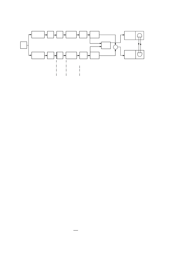
established according to guidelines derived from the knowledge of this system. A model of
the auditory–brain system (Figure 1) was proposed by Ando [1], correlating subjective
attributes with auditoryevoked potentials, including continuous brain wave (CBW), as
responding to variations of acoustical factors. This model consists of autocorrelators and
an interaural crosscorrelator acting on the pressure signals arriving at the two ears.
Furthermore, the model takes into account the specialization of the left and right human
hemispheres.

A theoryof primarysensations and spatial sensations responding to environmental

noise has been proposed [2] based on the model of an auditory–brain system. Primary
sensations}loudness, pitch, timbre and temporal duration- and spatial sensations}sub-
jective diffuseness, image shift of sound source and apparent source width (ASW)}can be
described bythe temporal and spatial factors extracted from the autocorrelation function
(ACF) and the interaural crosscorrelation function (IACF) respectively. It has been shown
that environmental noise can be characterized bythese factors [3–5]. Fundamental
subjective attributes for the sound field in a concert hall are accuratelydescribed bythe

0022-460X/02/$35.00

#

2002 Elsevier Science Ltd. All rights reserved.

model of auditory–brain system when taking into account the contributions of the ACF
and IACF mechanisms. For example, the speech intelligibilityof a spoken syllable with a
single reflection can be calculated from temporal factors extracted bythe ACF [6, 7]. In
concert hall acoustics, the theoryof subjective preference allows one to calculate the scale
values of subjective preference in terms of four orthogonal factors: the listening level

ðLLÞ;

the initial time-delaygap between the direct and the first reflection

ðDt

1

Þ; the subsequent

reverberation time

ðT

sub

Þ; and the interaural correlation coefficient ðIACCÞ [1].

Yamaguchi [8] carried out a dissimilarityexperiment studying the differences between

different seats in an existing concert hall and identified two significant factors: the sound
pressure level and the reverberation characteristics. Edwards [9] also tested dissimilarityby
studying the differences between different halls and reported that the early echo pattern,
the reverberation time RT ; and the volume level were the significant factors. Sato et al. [10]
and Cocchi et al. [11] confirmed the effectiveness of the theoryof subjective preference
through investigations in existing concert halls. Sato et al. [12] reconfirmed the
effectiveness of the theoryin an existing opera house.

In this study, dissimilarity judgments are obtained for a sound field with different source

locations on the stage of an existing hall. The obtained results were used to examine,
through multivariate analysis, the relationships between the dissimilarity judgments and
the physical factors based on the auditory–brain system of sound fields and the theory of
subjective preference.

2. PHYSICAL FACTORS BASED ON THE AUDITORY–BRAIN SYSTEM

2.1.

TEMPORAL FACTORS EXTRACTED FROM THE ACF

The power densityspectra in the neural activities in the left and right auditorypathways

show a sharpening effect [13, 14]. This information is sufficient to attain an approximation
of the ACF of the signals at both ears.

The ACF is defined by

F

p

ðtÞ ¼

1

2T

Z

þT

T

p

0

ðtÞp

0

ðt þ tÞ dt;

ð1Þ

Sound wave

p(t)

h

r

(r|r

0

,t)

e

r

(t)

c

r

(t) V

r

(x,

ω

)

I

r

(x')

Φ

rr

(

σ

)

h

l

(r|r

0

,t)

e

l

(t)

c

l

(t)

V

l

(x,

ω

)

I

l

(x')

Φ

ll

(

σ

)

Vibration Traveling

wave

Neural cord

Φ

lr

(

ν

)

+

r

l

Spatial
criterion

Temporal
criterion

Sound
source

Sound

field

External

canal

Eardrum,

bone chain

Basilar

membrane

Superior olivary

complex,

lateral lemniscus

Cochlear

nuclei

Medial

geniculate body

Auditory

cortex

Hair

cell

Inferior colliculus

Sharpening Correlation

mechanisms

Specialization

of human brain

Subjective

response

Figure 1. Model of the auditory–brain system with autocorrelation and interaural crosscorrelation

mechanisms and specialization of human cerebral hemispheres.

T. HOTEHAMA ET AL.

430

where p

0

ðtÞ ¼ pðtÞ*sðtÞ; with sðtÞ being ear sensitivity. For practical convenience, sðtÞ can

be chosen as the impulse response of an A-weighting network. Mouri et al. reported that
the integration interval 2T maybe set as 2T

30ðt

e

Þ

min

[15]. In this study, the integration

interval was set up with 2 s satisfying the condition. The ACF and power density spectrum
mathematicallycontain the same information.

Temporal factors extracted from the ACF are defined as follows. The first factor is the

effective duration of running ACF, t

e

:

This factor is defined bythe 10-percentile delay

representing repetitive features, or a kind of reverberation, within the source signal itself.
The t

e

is obtained from the decayrate for the range from 0 to

5 dB of the normalized

ACF. The second and third factors are the amplitude and the delaytime of the first
dominant peak of the normalized running ACF represented, respectively, as f

1

and t

1

:

It

was found that t

1

is the dominant factor of perceived pitch and f

1

relates to the intensity

of perceived pitch.

2.2.

SPATIAL FACTORS EXTRACTED FROM THE IACF

The auditory–brain model considers the interaural crosscorrelation mechanism between

the two auditorypathways [16]. To specifythe spatial characteristics of the sound field,
binaural measurements must be made. The fundamental spatial attributes of a sound field
are related to the IACF. The IACF between the sound signals at both ears, f

l

ðtÞ and f

r

ðtÞ;

is defined by

F

lr

ðtÞ ¼

1

2T

Z

þT

T

f

0

l

ðtÞf

0

r

ðt þ tÞ dt;

jtj 1 ms

ð2Þ

where f

0

l

ðtÞ and f

0

r

ðtÞ are approximatelyobtained bysignals f

l

ðtÞ and f

r

ðtÞ after passing

through the A-weighting network, which corresponds to the ear sensitivity, s

ðtÞ: The

external and middle ear maycharacterize the ear sensitivity.

The normalized IACF is defined by

f

lr

ðtÞ ¼

F

lr

ðtÞ

½F

ll

ð0ÞF

rr

ð0Þ

1=2

;

ð3Þ

where F

ll

ð0Þ and F

rr

ð0Þ are the ACFs at the origin of the time delayfor the left and right

ears respectively. These values correspond to the equivalent sound pressure level.

The spatial factors are extracted as fine structure of the running IACF. The first factor is

the geometrical mean of sound energies arriving at both ears, listening level, LL: This
factor is expressed by

LL

¼

10 log

½F

ll

ð0ÞF

rr

ð0Þ

1=2

F

ðref Þ

ð0Þ

;

ð4Þ

where

F

ðref Þ

ð0Þ ¼ ½F

ðref Þ
ll

ð0ÞF

ðref Þ
rr

ð0Þ

1=2

:

ð5Þ

Here, F

ðref Þ

ð0Þ is the geometrical mean of the ACF of binaurallyrecorded signals at t ¼ 0;

with the reference position indicated byequation (5). The selected reference position is 1 m
from the sound source.

The second factor is the IACC; which is the maximum value of the normalized IACF for

the time delay, within

1 ms, which correlates with subjective diffuseness [17, 18]. The

third and fourth factors are interaural time delay, t

IACC

;

and width of the running IACF,

W

IACC

:

The factor t

IACC

is interaural time delayat the maximum peak, which determines

IACC: This factor corresponds to the horizontal sound localization and the balance of the

DISSIMILARITY JUDGMENTS

431

sound field. The factor W

IACC

is defined as the time interval of the IACF spanning two

points within 10% of the maximum IACF value. This factor is stronglyrelated to the
apparent source width [6].

2.3.

ORTHOGONAL FACTORS OF THE SOUND FIELD FOR SUBJECTIVE PREFERENCE

As described in section 1, the theoryof subjective preference allows one to calculate the

scale value of subjective preference for a sound field in terms of the following four
orthogonal acoustical factors: the listening level, LL; the initial time-delaygap between the
direct and the first reflection, Dt

1

;

the subsequent reverberation time, T

sub

;

and the

magnitude of the IACF, IACC: These factors have been identified in systematic
investigations of sound fields through both computer simulation and listening tests
(paired-comparison tests) [1]. The subjective preference theoryhas also been validated by
tests in actual concert halls and opera houses [10–12].

3. METHOD

3.1.

SOURCE SIGNAL

A reverberation-free signal of orchestral music (‘‘Water Music’’ Suite No. 2-Alla

Hornpipe byHandel) was used as a source signal. The duration of the source signal
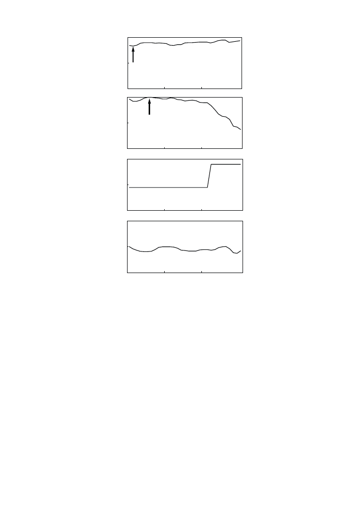
was 4 s. In subjective preference theory, a music source is characterized in terms
of the running autocorrelation function (ACF) of the source signal after passing
through an A-weighted network. The ACF analysis, with an integration interval
2T

¼ 20 s and running step of 100 ms, was carried out and factors Fð0Þ; t

e

;

t

1

;

and f

1

were extracted as shown in Figure 2. The value of

½Fð0Þ

max

is indicated byan

arrow at t

¼ 05 s. For the t

e

factor, the minimum value of the effective duration of

the source signal, which is stronglyrelated to the preferred conditions of temporal
factors, was 46 ms.

3.2.

DISSIMILARITY JUDGMENTS

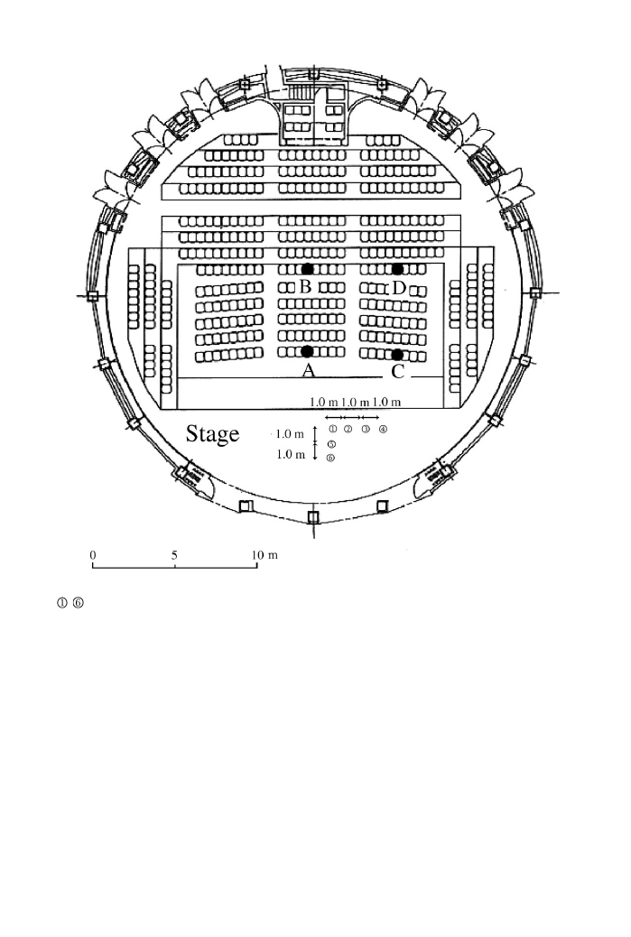
Dissimilarityjudgments were performed in a multi-purpose hall, the 400-seat ORBIS

Hall in Kobe as shown in Figure 3. Six loudspeakers were placed on the stage.
Twentylisteners were divided into four groups and seated at specific positions. Without
moving to different seats, dissimilarityjudgments were performed while switching six
source locations to obtain a scale value of dissimilarity. The listeners were asked to
judge the subjective difference as an overall impression between the paired stimuli on a
linear scale that has two extreme ends: ‘‘no difference’’ and ‘‘extremelydifferent.’’
The judgment conditions consisted of 15 pairs representing possible combinations of the
six sound fields at each listener’s location. The silent interval between paired stimuli was
1 s. Each pair of sound fields was separated byan interval of 5 s, and the pairs were
arranged in random order. Each session was repeated five times. In order to construct a
scale value of dissimilarityamong sound stimuli for the dependent variable, the original
data obtained bydissimilarityjudgment were categorized into seven categories. A method
of successive categories [19] was applied to the categorized data. The scale value of
dissimilarityfor each pair of source locations at seat positions A, B, C and D is listed
in Table 1.

T. HOTEHAMA ET AL.

432

3.3.

MEASUREMENTS OF ACOUSTICAL FACTORS

To measure the acoustical factors extracted from ACF and IACF, the music signal used

in the dissimilarityjudgments was reproduced from each loudspeaker used for
dissimilarityjudgments. The signal was recorded at each listening position, through two
microphones at both ear entrances of a person facing the center of the stage. To obtain the
impulse responses, an MLS signal was reproduced from each loudspeaker [16].

The running ACF and IACF of the recorded signals after passing the A-weighting

network were calculated byan integration interval 2T

¼ 20 s, and running step of 100 ms.

Values of t

1

and f

1

were calculated from running ACF analysis. The value of t

1

was

obtained bythe maximum peak of ACF in the time range between 50m s and 30 ms
corresponding to the human audible range. The value of f

1

defined bythe amplitude at t

1

was also determined. From the running IACF analysis, running values of LL; IACC;
t

IACC

;

and W

IACC

were calculated.

After obtaining the binaural impulse responses, values of Dt

1

and T

sub

were calculated.

The value of Dt

1

was defined bythe time difference between the arrival time of the direct

sound and that of the reflection, which is the maximum energyin the impulse responses.

1

10

100

-10

-5

0

0

5

10

0

0.5

0

1

2

3

1.0

Time [

s

]

Relative

Φ

(0) [dB]

τ

1

[

ms

]

φ

1

τ

e

[

ms

]

(

τ

e

)

min

= 46

ms

[

Φ

(0)]

max

(a)

(b)

(c)

(d)

Figure 2. Measured factors of running ACF of the source signal used in the experiment. The integration

interval of running ACF, 2T, was 2.0 s, with a 100 ms interval as a function of time. (a) t

e

;

(b) relative F

ð0Þ;

obtained as relative to the maximum value at t

¼ 05 s; (c) t

1

;

and (d) f

1

:

DISSIMILARITY JUDGMENTS

433

From the two Dt

1

values, the one with the largest amplitude obtained from binaural

impulse responses was selected as the Dt

1

of each loudspeaker position and each listening

position [20, 21]. For T

sub

;

500 Hz and 1 kHz octave band center frequencies were adopted,

since these frequencyranges are the dominant frequencies of the source signal.

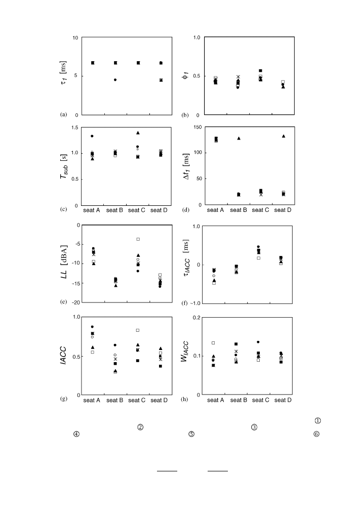
The measured temporal and spatial factors obtained byrunning ACF, IACF, and

binaural impulse response analyses are shown in Figure 4. The factors extracted from the
ACF and IACF were chosen from a short time interval centered on the time of

ðt

e

Þ

min

of

the source signal [22], because subjects were assumed to judge this instance as the most
sensitive and active portion of the source signal.

3.4.

MULTIPLE REGRESSION ANALYSIS

In order to determine a relationship between the scale values and physical factors

obtained by the measurement, the data were analyzed by multiple regression analysis. As

Figure 3. Plan of the ‘‘ORBIS Hall’’ in which dissimilarityjudgment was made. A–D: listeners’ locations.

–

: source locations changed in the paired comparison tests.

T. HOTEHAMA ET AL.

434

explanatoryvariables, a distance between paired stimuli was introduced bythe factors
extracted from the running ACF and the running IACF. In addition to these factors, the
orthogonal factors of the subjective preference of sound field were also taken into
consideration.

The distances between variables of each factor were calculated for each sound field. The

distance D

x

between the sound fields of a and b for each factor, x; was calculated in the

following manner. Subjective preference, in relation to temporal factors of sound fields,
was postulated to be subjectivelydetermined at the most active music segment, coinciding
with a minimum t

e

:

Therefore, factors extracted from running ACF and IACF were

chosen at the time frame where the source signal showed minimum t

e

[15, 22].

Temporal factors:

D

t

1

¼ jlogðt

1

Þ

a

logðt

1

Þ

b

j;

ð6Þ

D

f

1

¼ jlogðf

1

Þ

a

logðf

1

Þ

b

j:

ð7Þ

Spatial factors:

D

LL

¼ jðLLÞ

a

ðLLÞ

b

j;

ð8Þ

D

IACC

¼ jðIACCÞ

a

ðIACCÞ

b

j;

ð9Þ

D

t

IACC

¼ jðt

IACC

Þ

a

ðt

IACC

Þ

b

j;

ð10Þ

D

W

IACC

¼ jðW

IACC

Þ

a

ðW

IACC

Þ

b

j:

ð11Þ

Orthogonal factors for sound fields:

D

Dt

1

¼ log

Dt

1

½Dt

1

p

!

a

log

Dt

1

½Dt

1

p

!

b

;

ð12Þ

Table 1

Scale values of dissimilarity for each pair of source locations at seat positions A; B C and D

Pair of source locations

Seat position

Position A

Position B

Position C

Position D

1–2

1

4

0

8

0

8

0

9

1–3

1

9

1

7

1

8

1

6

1–4

2

3

2

0

2

5

2

4

1–5

0

7

0

9

0

8

0

7

1–6

1

3

1

0

1

4

1

0

2–3

0

8

0

6

1

2

1

3

2–4

1

2

1

2

2

2

2

0

2–5

1

6

1

2

0

7

0

9

2–6

1

8

1

4

0

8

0

6

3–4

0

5

0

4

1

6

1

2

3–5

2

1

1

9

1

8

1

7

3–6

2

1

2

0

1

4

1

7

4–5

2

4

2

0

2

2

2

1

4–6

2

2

2

1

2

0

2

0

5–6

0

4

0

4

0

9

0

8

DISSIMILARITY JUDGMENTS

435

D

T

sub

¼ log

T

sub

½T

sub

p

!

a

log

T

sub

½T

sub

p

!

b

;

ð13Þ

Figure 4. Measured physical factors at each listener’s location obtained from acoustical measurements. (a) t

1

;

(b) f

1

;

(c) T

sub

;

(d) D

1

;

(e) LL; (f) t

IACC

;

(g) IACC; and (h) WIACC: *; values measured for source location

;

*, values measured for source location

; m; values measured for source location

; &; values measured for

source location

; &: values measured for source location

; and *; values measured for source location

.

T. HOTEHAMA ET AL.

436

where D

Dt

1

and D

T

sub

are the distances of the nomalized values for the most preferred Dt

1

;

½Dt

1

p

and T

sub

;

½T

sub

p

respectively. The preferred values are expressed approximately as

½Dt

1

p

ð1 log

10

A

Þðt

e

Þ

min

; A

being the total pressure amplitude of all reflections, and

½T

sub

p

23ðt

e

Þ

min

:

The distances of temporal factors D

t

1

; D

f

1

; D

Dt

1

and D

T

sub

were

calculated using logarithmic values, since temporal factors are assumed to be perceived
according to the Weber–Fechner law. The explanatoryvariables in the analysis were: D

LL

;

D

t

1

; D

f

1

; D

IACC

; D

t

IACC

; D

W

IACC

; D

Dt

1

and D

T

sub

:

In the multiple regression analysis, the

distances for factors were combined linearly, using an expression given by

D

¼ aD

LL

þ bD

t

1

þ cD

f

1

þ dD

IACC

þ eD

t

IACC

þ fD

W

IACC

þ gD

Dt

1

þ hD

T

sub

;

ð14Þ

where D is a dependant variable to be calculated and a; b; c; d; e; f ; g and h are the co-
efficients to be evaluated. The coefficients were obtained bya step-wise regression method.
In this multiple regression model, no regression constant was included.

4. RESULTS

Prior to the multiple regression analysis, correlation coefficients among explanatory

variables were obtained as listed in Table 2. Results show that D

W

IACC

; D

LL

and D

IACC

highlycorrelated with D

t

IACC

(correlation coefficients with D

t

IACC

were 0

59; 056; and 054

respectively). The value of D

W

IACC

is a significant factor for determining ASW if source

signals of different frequencyranges are used [6], but had a minor effect in this experiment.
To avoid the effect of multicollinearity, which causes problems in estimating the effects of
explanatoryvariables on a dependant variable, D

W

IACC

was excluded from the explanatory

variables due to correlation with the significant factor D

t

IACC

:

By applying multiple regression analysis to the dependent variables and the explanatory

variables, normalized partial regression coefficients were obtained as listed in Table 3.

Table 3

Partial regression coefficients for significant factors obtained by multiple regression analysis

with normalized partial regression coefficients

D

t

1

D

f

1

D

t

IACC

D

Dt

1

D

T

sub

Partial regression coefficients

1

91

3

37

7

59

0

37

3

90

Normalized partial coefficients

0

10

0

15

0

69

0

08

0

17

p value

0

02

50

01

50

01

50

01

0

05

Table 2

Correlation coefficients between physical factors obtained from the acoustical measurements

D

LL

D

t

1

D

f

1

D

IACC

D

t

IACC

D

W

IACC

D

Dt

1

D

T

sub

D

LL

1

00

026

n

030

n

0

41

nn

0

56

nn

0

21

010

0

28

n

D

t

1

1

00

0

42

nn

0

08

018

023

0

13

034

nn

D

f

1

1

00

0

38

nn

028

n

004

0

23

029

n

D

IACC

1

00

0

54

nn

0

26

0

15

0

03

D

t

IACC

1

00

0

59

nn

005

0

04

D

W

IACC

1

00

002

011

D

Dt

1

1

00

025

D

T

sub

1

00

nn

: p

50

01;

n

: p

50

05:

DISSIMILARITY JUDGMENTS

437

D

LL

and D

IACC

were eliminated from the explanatoryvariables because p

01; namely,

these factors were not significant for dissimilarityin this experiment.

Normalized partial regression coefficients obtained here were 0

10 (D

t

1

; p

¼ 002), 015

(D

f

1

; p

50

01), 069 (D

t

IACC

; p

50

01), 008 (D

Dt

1

; p

50

01), and 017 (D

T

sub

;

p

¼ 005). The normalized partial regression coefficients indicated that the

effect of D

t

IACC

on dissimilaritywas the maximum (0

69). D

f

1

and D

Dt

1

also

significantlycontributed to the dissimilarity(p50

01).

In order to examine the relationships between the scale value obtained bydissimilarity

judgments and the dissimilaritycalculated bythe physical factors, the dissimilarityD was
obtained in the following manner:

D

191D

t

1

þ 337D

f

1

þ 759D

t

IACC

þ 037D

Dt

1

þ 390D

T

sub

:

ð15Þ

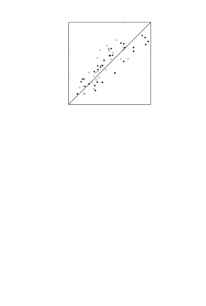
Figure 5 shows the relationship between scale values of dissimilarityat each seat position
and the calculated values byapplying the partial regression coefficients obtained from the
regression analysis for all seat positions. The correlation coefficients between scale values
of dissimilarityand calculated values at each seat position were 0

92 (p5001) at seat

position A, 0

79 (p5001) at seat position B, 090 (p5001) at seat position C, and 084

(p50

01) at seat position D. The total correlation coefficient between scale values of

dissimilarityand calculated values of dissimilarityfor all seats was 0

84 (p5001).

5. DISCUSSION

In this experiment, under the condition of changing source location, the effect of a

change in t

IACC

was dominant for dissimilarity. However the effects of changes

0

1.0

2.0

3.0

0

1.0

2.0

3.0

Calculated scale value

Scale v

alue of dissimilar

ity

Figure 5. Relationships between calculated scale values when applying equation (15) obtained by the

regression analysis for all seat positions and scale values of dissimilarity at each seat position (r

¼ 084; p5001).

*

;

values obtained at seat position A (r

¼ 092; p5001); *, values obtained at seat position B (r ¼ 079;

p50

01); m; values obtained at seat position C (r ¼ 090; p5001); &; values obtained at seat position D

(r

¼ 084; p5001).

T. HOTEHAMA ET AL.

438

in D

LL

and D

IACC

could not be taken into account because of the high correlation

with D

t

IACC

:

The most important result was that D

f

1

and D

Dt

1

;

which are temporal

factors, significantlycontributed to dissimilarity

. This implies that subjects judged

dissimilaritybynot onlya change in spatial factors but also a change in temporal
factors. The subjective preference theory[1] predicts that both temporal and spatial
factors of sound fields affect subjective preference when forming an overall impression of a
sound field. The same effects maybe obtained for dissimilarity

, based on the overall

responses.

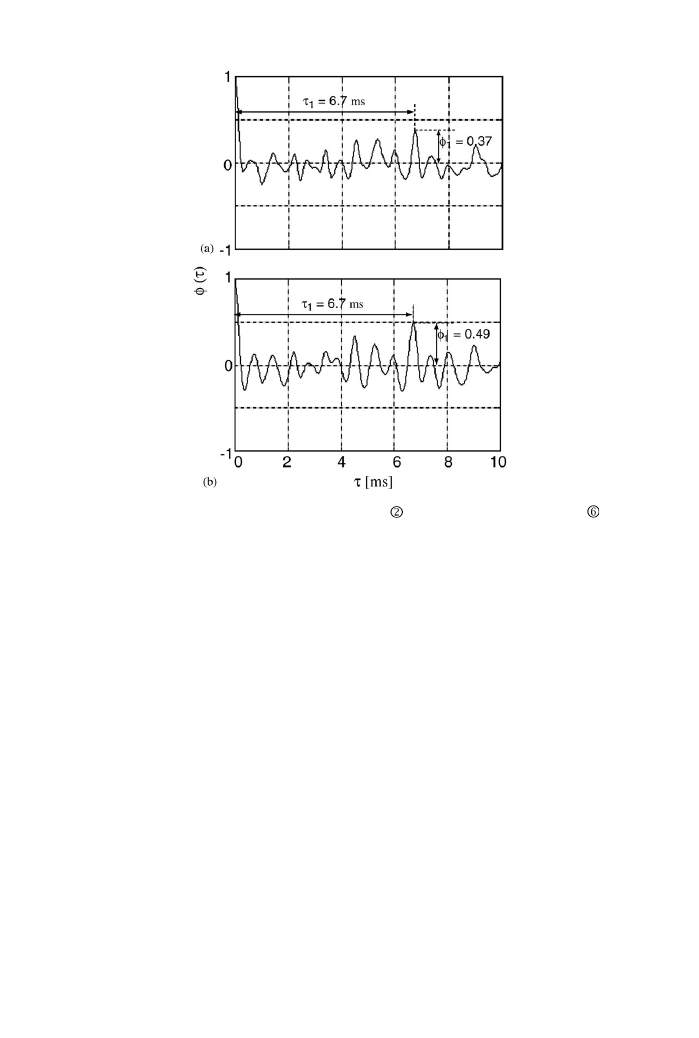
Figure 6 illustrated the examples of the running ACF of source locations 2 and 6 at seat

position B. A difference can be seen in the ACFs affected bythe different transmission
characteristics of sound fields. As for the effect of f

1

on dissimilarity, it can be said that

the subjects perceive the difference in sound fields through the difference in ACF. This
result corresponds to those obtained byYost [23], who demonstrated that pitch perception
of iterated rippled noise is dominantlyaffected bythe first ACF peak of the stimulus
signal.

6. CONCLUDING REMARKS

Results of multiple regression analysis show that psychological distance can be

accuratelydescribed bythe temporal and spatial factors obtained byACF and IACF as

Figure 6. Examples for ACF waveform. (a) source location

at seat position B; source location

at seat

position B.

DISSIMILARITY JUDGMENTS

439

well as the orthogonal factors extracted from binaural impulse response analyses based on
the auditory–brain system and the subjective preference theory.

ACKNOWLEDGMENTS

The authors wish to thank the staff of our laboratoryfor their cooperation during

experiments. We also thank the students who participated in the experimental
sessions.

REFERENCES

1. Y. Ando 1998 Architectural Acoustics } Blending Sound Sources, Sound Fields, and Listeners.

New York: AIP/Springer-Verlag.

2. Y. Ando 2001 Journal of Sound and Vibration 241, 2–18. A theoryof primarysensations

measuring environmental noise.

3. H. Sakai, S. Sato, N. Prodi and R. Pompoli 2001 Journal of Sound and Vibration 241, 57–68.

Measurement of regional environmental noise byuse of a PC-based system. An Application to
the noise near Airport ‘‘G. Marconi’’ in Bologna.

4. K. Fujii, Y. Soeta and Y. Ando 2001 Journal of Sound and Vibration 241, 57–68. Acoustical

properties of aircraft noise measured bytemporal and spatial factors.

5. H. Sakai, H. Hotehama, N. Prodi, R. Pompoli and Y. Ando 2002 Journal of Sound and

Vibration 250, 9–21. Diagnostic system based on human auditory–brain model for measuring
environmental noise}an application to railwaynoise.

6. Y. Ando, H. Sakai and S. Sato 1999 in Computational Acoustics in Architecture (J. J. Sendra,

editor). Fundamental subjective attributes of sound fields based on the model of auditory–brain
system. Acoustical properties of aircraft noise measured by temporal and spatial factors.
Ashurdt Lodge: Computational Mechanics Publication, WIT Press.

7. Y. Ando, H. Sakai and S. Sato 2000 Journal of Sound and Vibration 232, 101–127. Formulae

describing subjective attributes for sound fields based on a model of the auditory–brain system.

8. K. Yamaguchi 1972 Journal of Acoustical Society of America 52, 1271–1279. Multivariate

analysis of subjective and physical measurements of hall acoustics.

9. R. M. Edwards 1974 Acustica 30, 183–195. A subjective assessment of concert hall

acoustics.

10. S. Sato, Y. Mori and Y. Ando 1997 in Music and Concert Hall Acoustics (Y. Ando and D.

Noson, editors). On the subjective evaluation of source locations on the stage bylisteners.
London; Academic Press: Chapter 12.

11. A. Cocchi, A. Farina, M. Garai and L. Tronchin 1997 in Music and Concert Hall Acoustics

(Y. Ando and D. Noson, editors). Computer assisted methods and acoustic quality: recent
application cases. London: Academic Press; Chapter 8.

12. S. Sato, H. Sakai and N. Prodi 2002 Journal of Sound and Vibration 258, 543–555, this issue.

Subjective preference for sound sources located on the stage and in the orchestra pit of an opera
house.

13. Y. Katsuki, T. Sumi, H. Uchiyama and T. Watanabe 1958 Journal of Neurophysiology 21,

569–588. Electric responses of auditoryneurons in cat to sound stimulation.

14. N. Y.-S. Kiang 1965 Discharge Pattern of Single Fibers in the Cat’s Auditory Nerve. MA,

Cambridge; MIT Press.

15. K. Mouri, K. Akiyama and Y. Ando 2001 Journal of Sound and Vibration 241, 87–95.

Preliminarystudyon recommended time duration of source signals to be analyzed, in relation to
its effective duration of the auto-correlation function.

16. M. Sakurai, S. Aizawa, Y. Suzumura and Y. Ando 2000 Journal of Sound and Vibration 232,

231–237. A diagnostic system measuring orthogonal factors for sound fields in a scale model of
auditorium.

17. Y. Ando and Y. Kurihara 1986 Journal of Acoustical Society of America 80, 833–836.

Nonlinear response in evaluating the subjective diffuseness of sound fields.

18. P. K. Singh, Y. Ando and Y. Kurihara 1994 Acustica 80, 471–477. Individual subjective

diffuseness responses of filtered noise fields.

19. W. S. Torgerson 1958 Theory and Methods of Scaling. New York: Wiley.

T. HOTEHAMA ET AL.

440

20. J. Atagi, R. Weber and V. Mellert 2001 Proceedings of the 17th International Congress on

Acoustics, Roma, Italy. Effects of modulated delaytime of reflection on the autocorrelation
function and perception of the echo.

21. Y. Ando and D. Gottlob 1979 Journal of Acoustical Society of America 65, 524–527. Effects of

earlymultiple reflection on subjective preference judgments on music sound fields.

22. Y. Ando, T. Okano and Y. Takezoe Journal of Acoustical Society of America 89, 644–649. The

running autocorrelation function of different music signals relating to preferred temporal
parameters of sound fields.

23. W. A. Yost 1996 Journal of Acoustical Society of America 100, 3329–3335. Pitch strength of

iterated rippled noise.

DISSIMILARITY JUDGMENTS

441