Journal of Sound and <ibration (2000) 232(1), 157}169
doi:10.1006/jsvi.1999.2691, available online at http://www.idealibrary.com on

INDIVIDUAL SUBJECTIVE PREFERENCE OF LISTENERS

TO VOCAL MUSIC SOURCES IN RELATION TO THE

SUBSEQUENT REVERBERATION TIME OF SOUND FIELDS

H. S

AKAI AND

Y. A

NDO

Graduate School of Science and ¹echnology, Kobe ;niversity, Kobe, 657-8501, Japan

AND

H. S

ETOGUCHI

Kirishima International Concert Hall, Kagoshima, 899-6603, Japan

(Accepted 30 June 1999)

The purpose of this study is to evaluate individual di!erences and intra-

individual changes of subjective preference of simulated sound "eld judged by
listeners in changing subsequent reverberation time ¹QS@ using a vocal source.

A great deal of e!ort has been made studying subjective preferences by using music
or speech. Subjective preference tests were conducted by changing ¹QS@, which is

one of the four orthogonal-objective parameters of sound "eld.

2000 Academic Press

1. INTRODUCTION

It is well known that subjective preference evaluation of sound "elds is
accompanied by individual di!erences [1, 2]. Using results from subjective
preference tests in relation to orthogonal parameters of sound "elds, each listener
can select his or her optimum seat in a given concert hall [3]. Psychological
evaluations in relation to preference of sound "elds have been considered by their
global results as an average of many subjects and also for each subject [4, 5]. In
order to clarify individual di!erences in subjective preference, intra-individual
changes should be investigated. The variations of preference evaluations caused by
aging, seasons, time (morning, evening or night), a certain period of time during the
repetition of psychological tests, and so on, are considered. As a typical example,
a person's hearing level may be a!ected by aging. In this study, the variation of
preference evaluations during the repetition of psychological tests is applied to
intra-individual changes.

In a previous study on intra-individual changes in SP¸ by using a music source

[6], it was found that subjects with large

a values (see later for the de

"nition of

a)

have smaller intra-individual changes than subjects with small ones, and the range
of the variation of preferable SP¸ is small.

0022-460X/00/160157#13 $35.00/0

2000 Academic Press

Subjective preference evaluations for intra-individual changes are identi"ed by

two factors from subjective preference curves obtained from paired-comparison
tests as well as their global case and individual di!erences. One factor is the value at
the most preferred parameter, which coincides with the peak of the preference
curves. The other is the sharpness of the curve,

a, which is an index of the degree of

preference; see equation (3). For a unit variation of a parameter, the scale value for
a certain subject with a large

a value changes more rapidly than that of other

subjects with a small

a. Procedures for obtaining these parameters are described in

the next section.

For vocal music, which is one of the main components of performances in opera

houses, this study evaluates listener's individual di!erences and intra-individual
changes in subjective preference to various simulated sound "elds. Subjective
preference tests were conducted by changing subsequent reverberation time, ¹QS@,

which is one of the four orthogonal parameters that describe subjective preference
to sound "elds. The value of ¹QS@ is de"ned by the decay rate of the sound pressure

level after arrival of the "rst re#ection until !60 dB. For calculating scale values of
tests, a simple method of calculating individual subjective preference was
adopted [7].

2. EXPERIMENTAL METHOD

2.1.

CHARACTERISTICS OF A SOUND SOURCE

The sound source used was an initial 6)0 s piece of a solo performance of

a soprano single (&&O mio babbino caro'' from &&Gianni Schicchi'' composed by
G. Puccini) recorded in an anechoic chamber. Values of

qC, which is the e!ective

duration of the normalized autocorrelation function (ACF),

(q), of a short-time

moving ACF or running ACF (2¹"2)0 s with the interval of 100 ms) [8] for
the initial 6)0 s part of the source reproduced in the listening semi-anechoic
chamber, were calculated. The waveform and values of running

qC are indicated in

Figures 1(a) and (b) respectively. The short-time moving ACF was calculated in
order to obtain the minimum of its running

qC, which represents the most rapid

movement of music, activating the left cerebral hemisphere [9]. As indicated
in Figure 1(c), the running

qC is practically obtained by calculating the decay

rate extrapolated in the range from 0 dB, at the origin, to !5 dB. The 2)0 s
duration corresponds to the psychological present [10] and the minimum
duration of signals corresponds to response to any subjective attributes. The most
preferred ¹QS@ averaged for a number of listeners can be calculated by using the

equation [11]

[¹QS@]N+23(qC)KGL,

(1)

where (

qC)KGL is the minimum value of qC for the source music. The calculation of

global preferable subsequent reverberation time [¹QS@]N is about 0)53 s, which is

shorter than usual music sources but longer than that of speech signals.

158

H. SAKAI E¹ A¸.

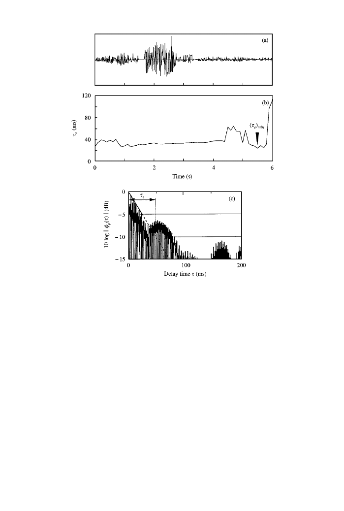
Figure 1. The e!ective duration

qC of the running normalized autocorrelation function of the vocal

source used in the tests. The integration interval, 2¹, is 2)0 s. The waveform of the vocal source
reproduced in the listening-semi-anechoic room (a). The minimum value of

qC, which is the most active

part of the source containing important information and in#uencing subjective responses to
the temporal criteria, is found to be about 23 ms (b). An example of determining the value of

qC "tting

0 to !5 dB of the envelope (c).

2.2.

PSYCHOLOGICAL EXPERIMENT

Paired-comparison tests were conducted in a semi-anechoic room (see Figure 2).

With [¹QS@]N taken to be about 0)53 s as mentioned above, the subsequent

reverberation time ¹QS@ of the sound "eld was changed from 0)1 to 1)6 s (see Table 1).

The conditions of the other orthogonal parameters were "xed as indicated in Table
1. The initial time-delay gap between the direct sound and the "rst re#ection,

Dt,

was "xed at 14 ms near to the most preferred value [

Dt]N+(1!logA)

(

qC)KGL+16 ms. The IACC is near to unity because the two loudspeakers were set in

front of the subjects. The total amplitude of re#ections A is kept constant at 2)0. The
duration of each stimulus presented to subjects was 6)0 s. The time interval between
the two stimuli in a pair was 1)0 s and between each pair lasted 4)0 s. There are 10

INDIVIDUAL SUBJECTIVE PREFERENCE

159

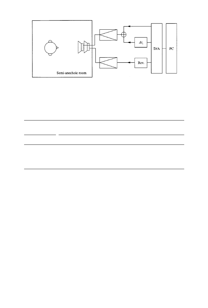
Figure 2. Experimental set-up of subjective preference tests controlling both the initial time delay

gap between the direct sound and the "rst re#ection,

Dt, and the subsequent reverberation time, ¹QS@.

T

ABLE

1

Subsequent reverberation time ¹QS@ values under ,xed conditions of SP¸, Dt

IACC and the total amplitude of re-ections A

Factors varied

or "xed

Value(s) of each factor

¹QS@

(s)

0)1

0)2

0)4

0)8

1)6

SP¸

[dB(A)]

75)0$0)2

Dt

(ms)

14

IACC

+

1)0

A

+

2)0

pairs in a series which are all the available pairs for "ve sound "elds
(N(N!1)/2"10, N"5). A series of 20 paired-comparison tests were conducted
on each subject. The number of subjects was eight (subjects A}H: seven males and
one female; 21}26 years old). The stimuli were produced by two loudspeakers
placed in front of the subjects in the listening room. The distance between a subject
and the loudspeakers was 0)8$0)01 m. One speaker provides a direct sound and
the "rst re#ection, and the other provides reverberation including some initial
re#ections. Subjects were required to select the most preferred sound "eld of the
two they listened to.

2.3.

CALCULATION OF THE SCALE VALUE

We used the subjective responses from each subject to calculate the scale values

of preference for each sound "eld. The procedure for calculating scale values of
preference is outlined in Table 2. The scores for each presented pair are obtained by
giving scores of #1 and 0 corresponding to positive and negative judgments

160

H. SAKAI E¹ A¸.

T

ABLE

2

Example of obtaining scale values of sound ,elds calculated by equation (2) (subject G)

¹QS@

(s)

0)1

0)2

0)4

0)8

1)6

¹G

SG

0)1

10

3

2

0

15

30

!

0)501

0)2

17

10

1

0

18

46

!

0)100

0)4

18

19

10

0

17

64

0)351

0)8

20

20

20

10

19

89

0)978

1)6

5

2

3

1

10

21

!

0)727

respectively. For example, the score of the pair (0)4 s, 0)1 s) listed in Table 2 is 18.
This result shows that the subject prefer the sound "eld with 0)4 s 18 times of 20
times to the sound "eld with 0)1 s. The ideal preference score comparing sound

"elds with same value of ¹

QS@

is 0)5 as &&a tie'' [12] and, thus, the scores of diagonal

set in the table are 10 (against 20 times). The values of ¹G represent the total score.

The scale value of subjective preference for sound "eld i can be obtained by
assuming a normal distribution of preference judgment [7]; i.e.,

SG+(2n(2¹G!N)/2N.

(2)

Here N indicates the number of sound "elds ("5). This approximate equation is
derived from case V of Thurstone's law of comparative judgment [13] and holds
the linear domain of a normal ogive (0)05(P(0)95, P: probability judged). Each
subject's most preferred value, [¹QS@]NK, is obtained at the peak of the preference

curves. The formula used for "tting scale values of preference is given by [11]

S+!

a"x"@,

(3)

where

x"log(¹QS@/[¹QS@]N).

(4)

The value of [¹QS@]N is obtained by equation (1). Weighting coe$cient a indicates

the sharpness of curve. If a subject has a large

a value, the degree of preference

decreases sharply as the value of ¹QS@ is apart from the preferred value. The value of

the weighting coe$cient

b may be found to be around three halves, in regard to

subjective preference of sound "elds [1, 11]. Weighting

a can thus be obtained.

The individual

a value can be obtained from the average of preference score ¹G in

Table 2 for all series of tests and all subjects.

A test of goodness of "t to ensure the "tness of the model is adopted. The value of

j represents the poorness of the model (0(j(1) and is de

"ned by

j"

GH

"SG!SH".MMP

GH

"SG!SH", 0)j)1,

(5)

INDIVIDUAL SUBJECTIVE PREFERENCE

161

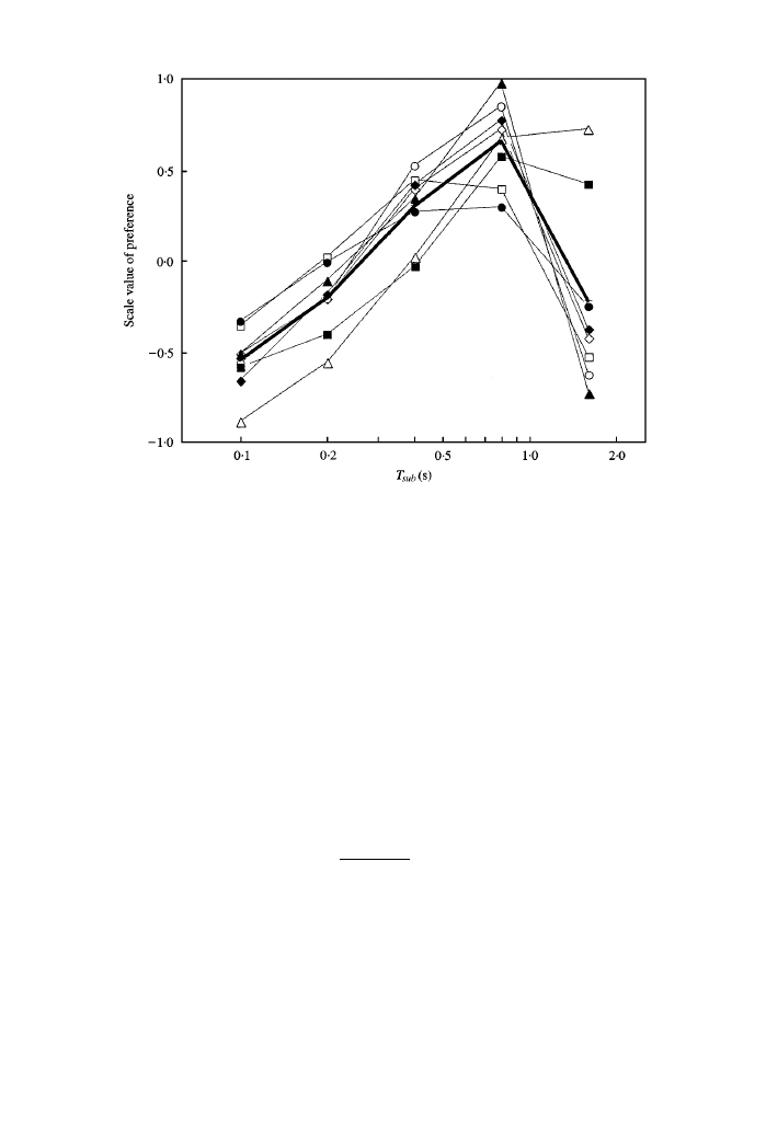
Figure 3. Scale values of preference for each subject as a function of ¹QS@. Di!erent symbols indicate

results from di!erent subjects:

䉫, 䊊, 䉭, 䊐, 䉬, 䊉, 䉱, and 䊏 for subjects A through H respectively. The

bold line represents the averaged values.

where

"SG!SH".MMP"SH!SG'0, if >G"0,"0, if >G"1.

(6)

The value of

j corresponds to the average error of the scale value. This should be

small enough: for example, less than 10%. The value of >G represents the score for

each alternative judgment.

Another observation is that, when the poorness number is K, satisfying the

condition expressed by upper part of equation (6), then the percentage of violations
d is de"ned by

d"

2K

N(N!1)

;100.

(7)

3. RESULTS

3.1.

INDIVIDUAL DIFFERENCES AND GLOBAL CASE

The measured results of the scale values of preference as the function of the

¹QS@

for each subject and its global case are indicated in Figure 3. In this "gure,

di!erent symbols represent the results from each subject, and the bold line

162

H. SAKAI E¹ A¸.

T

ABLE

3

<

alues of [¹QS@]NK, aQ ( for ¹QS@([¹QS@]NK) and aJ( for ¹QS@'[¹QS@]NK) obtained for

global and each subject

Subject

Global

A

B

C

D

E

F

G

H

[¹QS@]NK (s) 0)78

0)81

0)69

1)22

0)55

0)74

0)59

0)81

1)07

aQ

1)53

1)53

2)02

1)61

1)38

1)86

0)97

1)87

1)40

aJ

5)24

7)65

7)09

1)69

3)27

6)19

2)12

11)04

4)08

T

ABLE

4

Result of analysis of variance (ANO<A). Individual di+erences are observed in

log([¹QS@]NK/[¹QS@]N) (p(0)05) and aQ(p(0)01)

Factor

F-ratio

p-value

log([¹QS@]NK/[¹QS@]N)

2)740

0)0285*

aQ

4)495

0)0022**

aJ

1)929

0)1054

Note: *p(0)05; **p(0)01.

represents the averaged value as the global result. As the sharpness of the curves are
found to be di!erent for each side of the preference curves' peaks, two values of

a for

both sides of the peak are considered as

aQ for ¹QS@([¹QS@]NK and aJ for

¹QS@'

[¹QS@]NK in equation (3). The range of most preferred values of subsequent-

reverberation time [¹QS@]NK obtained for all subjects in the tests was between 0)55

and 1)22 s. The largest value of

aQ was 2)02 (subject B) and the smallest one was 0)97

(subject F). On the other hand, the largest value of

aJ was 11)04 (subject G) and the

smallest one was 1)69 (subject C). The values of

aJ are always greater than those of

aQ, for all subjects tested without exception. The experimental measurements of

[¹QS@]NK, aQ, and aJ for each subject as well as global results are listed in Table 3.

The goodness of "t of this model for each subject, expressed using

j in equation (5)

representing the poorness of the model for each subject, gives zero except for 0)04
for subject B. The values of d in equation (7) were also zero for all subjects except for
0)1 for subject B. These small values indicate that a consistent model is achieved for
this test. Individual di!erence is found in log([¹QS@]NK/[¹QS@]N) (p(0)05) and aQ

(p(0)01) by use of analysis of variance (ANOVA), as shown in Table 4. The
method of ANOVA is referred to in Appendix II. For example, subject B (

aQ"2)02

and

aJ"7)09) and subject G (aQ"1)87 and aJ"11)04) show a sharper preference

curve than subject D (

aQ"1)38 and aJ"3)27) and subject F (aQ"0)97 and

aJ"2)12). In the global results obtained in the tests, [¹QS@]NK was 0)78 s, and values

of

aQ and aJ were 1)53, and 5)24 respectively. This means that for ¹QS@ greater than

the most preferred value, preference curves are sharper than those for ¹QS@ less than

the most preferred value.

INDIVIDUAL SUBJECTIVE PREFERENCE

163

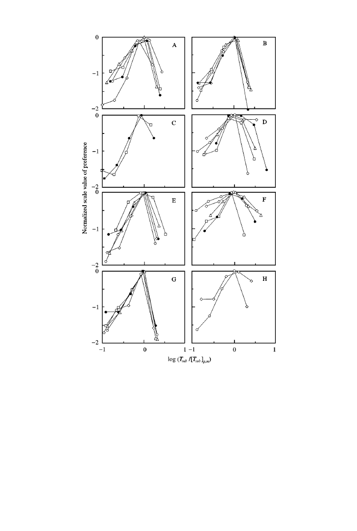
Figure 4. Individual scale values of preference obtained from every four series of each subject as

a function of the normalized subsequent reverberation time. The peaks of the curves are shifted to the
origin without any loss of information. Di!erent symbols indicate values of a di!erent series of tests:

䉫, 䊊, 䉭, 䊐, and 䊉.

3.2.

INTRA-INDIVIDUAL CHANGES

The measured results of intra-individual changes of subjective preference for each

subject (A}H) are indicated in Figure 4. In this "gure, di!erent symbols represent
the results in every four series of tests performed over three or four days. Each peak
value of the preference curves is shifted to the origin without losing any
information, because a scale value is a relative and a linear scale. For example,

164

H. SAKAI E¹ A¸.

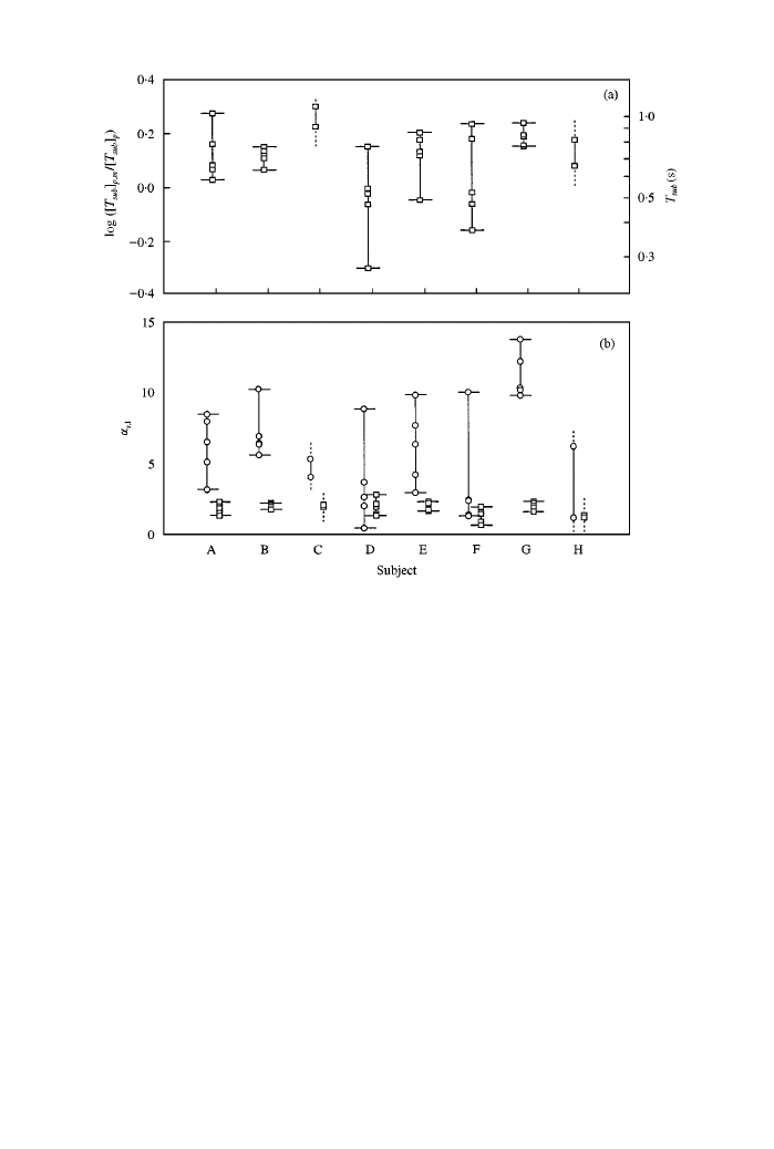
Figure 5. Intra-individual changes of log([¹QS@]NK/[¹QS@]N) (a); aQ (䊐) and aJ (䊊) for each subject (b).

Broken lines show that preferred values are out of the range between 0)1 s and 1)6 s

curves of subjects B and G are almost the same, but those of subjects D and F are
greatly changed over "ve sets of tests. There are only two curves of both subjects
C and H, because the other three sets could not be obtained. The measured results
of log([¹QS@]NK/[¹QS@]N), aQ, and aJ for each set are indicated in Figure 5. Subjects

with large

a values, like subjects B and G, have small intra-individual changes with

respect to values of log([¹QS@]NK/[¹QS@]N). Standard deviations of these factors

obtained from each set of tests are listed in Table 5. The values of subjects C and H,
with only two sets, are not listed. Subject B (0)033) and subject G (0)035) have the
two smallest standard deviations of all subjects, and subject D (0)163) and subject
F (0)168) have larger standard deviations. In relation to those of

aQ and aJ, subject

B (

aQ: 0)16; aJ: 1)84) and subject G (aQ: 0)26; aJ: 1)68) have smaller standard deviations

as well as the values of log([¹QS@]NK/[¹QS@]N). On the other hand, subject D (aQ: 0)61;

aJ: 3)21) and subject F (aQ: 0)55; aJ: 3)67) have larger standard deviations.

4. DISCUSSION

Values of both

aQ and aJ of subjects B and G were greater than those of the other

subjects and have almost the constant values, and these values of subjects D and

INDIVIDUAL SUBJECTIVE PREFERENCE

165

T

ABLE

5

Standard deviations of log([¹QS@]NK/[¹QS@]N), aQ and aJ for each subject

Subject

log([¹QS@]NK/¹QS@]N)

aQ

aJ

A

0)098

0)36

2)17

B

0)033

0)16

1)84

C

}

}

}

D

0)163

0)61

3)21

E

0)097

0)29

2)74

F

0)168

0)55

3)67

G

0)035

0)26

1)68

H

}

}

}

Note: Data for subjects C and H were not obtained.

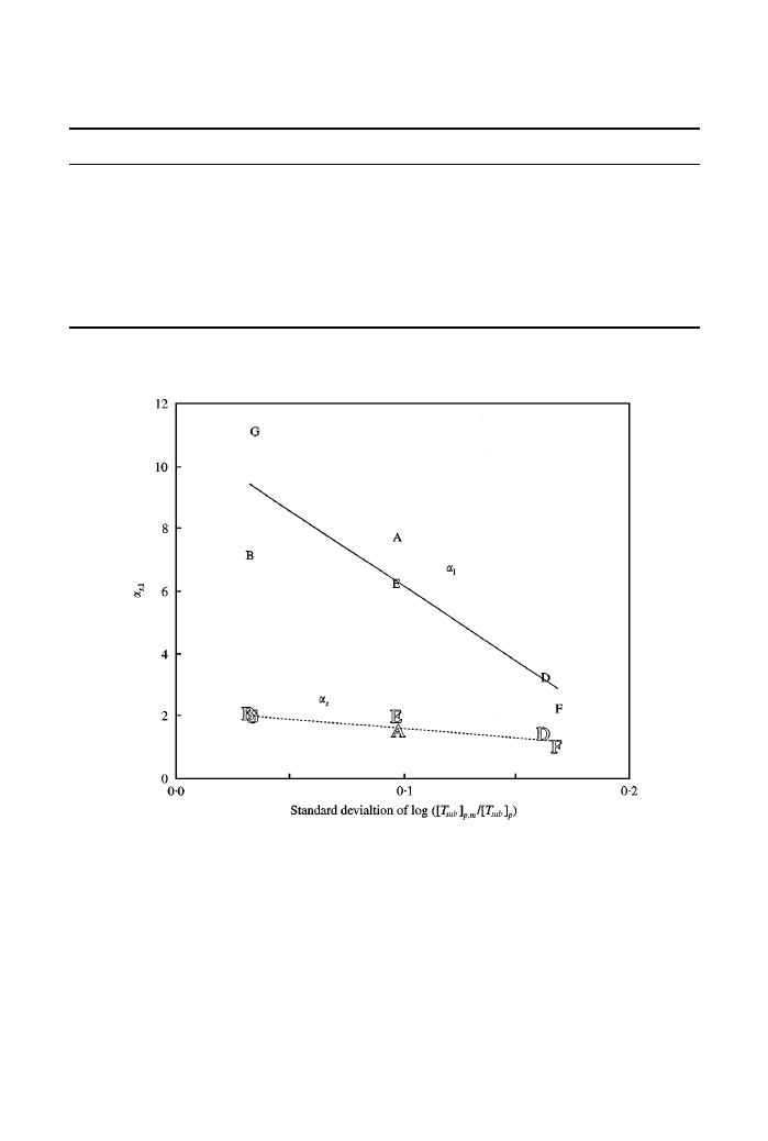
Figure 6 .Relationship between

aQ and aJ, and standard deviation of preferred reverberation time

on a logarithmic scale, log([¹QS@]NK/[¹QS@]N), for each subject (except for subjects C and H). Solid line

represents

aJ (subjects A}H with R"0)76) and dotted line represents aQ (subjects }' with

R

"0)70).

F are signi"cantly di!erent in each set. The results of log([¹QS@]NK/[¹QS@]N), the

values of

aQ, and aJ in every four series for each subject are indicated in Figure 4. On

both sides of the peaks, for subjects who have larger

a, such as subjects B and G, the

standard deviations of log([¹QS@]NK/[¹QS@]N) for each set are small. On the other

hand, for subjects who have smaller

a, such as subjects D and F, the preferable

¹QS@

values are larger: 0)163 and 0)168 respectively.

166

H. SAKAI E¹ A¸.

Relationship between the standard deviations of log([¹QS@]NK/[¹QS@]N), aQ and aJ

values for each subject (except subjects C and H) are plotted in Figure 6. Subjects
with large

a values, such as subject B or subject G, have smaller intra-individual

changes, so that the standard deviations of preferable ¹QS@ is small. On the other

hand, subjects with small

a values such as subjects D and F show minor preferences

as ¹QS@ changed. This result is similar to that of previous results for SP¸ [6].

The value of [¹QS@]N calculated by using equation (1) with (qC)KGL ("23 ms) is

0)53 s. For the global subjects, the value of [¹QS@]NK obtained by the tests was 0)78 s,

longer than the calculated value.

5. CONCLUSION

Subjects with large

a values indicate smaller intra-individual changes, so the

standard deviation of log([¹QS@]NK/[¹QS@]N) is small. On the other hand, subjects

with small

a values without sharp curves show minor preference as ¹QS@ changed.

The averaged value of preferred ¹QS@ for vocal sources was 0)78 s, which is greater

than the value (0)53 s) calculated by equation (1). Individual di!erences are
observed in values of log([¹QS@]NK/[¹QS@]N) and aQ but not in value of aJ.

ACKNOWLEDGMENT

The authors wish to thank Mrs. Mikiyo Setoguchi as a soprano singer for her

cooperation in recording source signals. This work is supported by the Ministry of
Education, Grant-in-Aid for Scienti"c Research (C), 9838022, 1998.

REFERENCES

1. Y. A

NDO

1998 Architectural Acoustics}Blending Sound Sources, Sound Fields, and

¸

isteners New York: Springer-Verlag, chapter 9.

2. Y. A

NDO

and P. K. S

INGH

1997 Music and Concert Hall Acoustics, Conference

Proceedings of MCHA 1995 (Y. Ando, D. Noson, editors). London: Academic Press,
chapter 4. Global subjective evaluation for design of sound "elds and individual
subjective preference for seat selection.

3. M. S

AKURAI

, Y. K

ORENAGA

and Y. A

NDO

1997 Music and Concert Hall Acoustics,

Conference Proceedings of MCHA 1995 (Y. Ando, D. Noson, editors). London:
Academic Press, chapter 6. A sound simulation system for seat selection.

4. Y. A

NDO

, M. O

KURA

and K. Y

UASA

1982 Acustica 50, 134}141. On the preferred

reverberation time in auditoriums.

5. Y. A

NDO

, K. O

TERA

and Y. H

AMANA

1983 ¹he Journal of Acoustical Society of Japan 39,

89}95. Experiments on the universality of the most preferred reverberation time for
sound "elds in auditoriums (in Japanese with English abstract).

6. H. S

AKAI

, P. K. S

INGH

and Y. A

NDO

1997 Music and Concert Hall Acoustics, Conference

Proceedings of MCHA 1995. (Y. Ando, D. Noson, editors). London: Academic Press,
chapter 13. Inter-individual di!erences in subjective preference judgements of sound

"elds.

7. Y. A

NDO

and P. K. S

INGH

1996 Memoirs of the Graduate School of Science and

¹

echnology, Kobe ;niversity 14-A, 57}66. A simple method of calculating individual

subjective responses by paired-comparison tests.

INDIVIDUAL SUBJECTIVE PREFERENCE

167

8. Y. A

NDO

, T. O

KANO

and Y. T

AKEZOE

1989 Journal of the Acoustical Society of America

86, 644}649. The running autocorrelation function of di!erent music signals relating to
preferred temporal parameters of sound "elds.

9. K. M

OURI

, K. A

KIYAMA

and Y. A

NDO

1998 Journal of Sound and <ibration (Special Issue

on Opera House Acoustics). Relationship between subjective preference the alpha-brain
wave in relation to the initial time delay gap with vocal music.

10. P. F

RAISSE

1982 ¹he Physiology of Music (D. Deutsch, editor). Orland, Fl: Academic

Press, chapter 6, Rhythm and tempo.

11. Y. A

NDO

1985 Concert Hall Acoustics. New York: Springer-Verlag, chapters 3 and 4.

12. W. A. G

LENN

and H. A. D

AVID

1960 Biometrics 16, 86}109. Ties in paired-comparison

experiments using a modi"ed Thurstone}Mosteller model.

13. L. L. T

HURSTONE

1927 Pschological Review 34, 273}286. A law of comparative

judgment.

14. H. S

AKAI

, H. S

ETOGUCHI

and Y. A

NDO

1997 Journal of the Acoustical Society of America

102, 3187. Subjective preference judgments of simulated sound "eld by listeners for
sound source in opera performance.

APPENDIX A

For calculating the scale values of preference, a simple method [7] was used as an

approximation for case V of Thurstone's law of comparative judgment [13]. It must
be noted that the estimated scale value obtained by this method is smaller than the
result estimated by the case V of Thurstone's law, though high correlation
coe$cient (r"0)99) was found between the scale values obtained from both
methods. The results of two recent psychological tests [14], including this test with

"ve sound "elds show that the correlation ratio becomes about 1)26. This ratio may

be mainly changed by the number of sound "elds and individual di!erences.

APPENDIX B

In this article, the one-way analysis of variance (ANOVA) is adopted in order to

evaluate

individual

di!erences

in

relation

to

the

values

of

factors,

log([¹QS@]NK/[¹QS@]N), aQ and aJ as shown in Table 4. Its de"nitions and usage are

brie#y described here. By use of the ANOVA, signi"cance tests of individual
di!erences are conducted for the each factor which is categorized by each subject as
levels.

At "rst, two hypotheses are set as follows. As the null hypothesis, each group,

categorized by each subject, is considered to be sampled from one population. In
this hypothesis, an individual di!erence is reserved. As the alternative hypothesis,
each group is considered to be sampled from di!erent populations. In this case, the
null hypothesis is rejected and alternative hypothesis is adopted. Hence individual
di!erence is accepted.

The values of F-ratio, F, are given as ratios of between-individuals variance and

residual variance, calculated by the following equations:

F"s

/s#, s"S/df, s#"S#/df#.

168

H. SAKAI E¹ A¸.

Here the values of S and S# are given as a square-sum due to between-individuals

variation and residual sum of squares respectively. The values of df and df# are

degrees of freedom of between-individuals variation and residual respectively. The
F-ratio is a statistical value representing the di!erence among groups. If the null
hypothesis is correct, the expected value of the F-ratio approaches unity, and the
individual di!erence is reserved. If the F-ratio is greater than unity, it is considered
that individual di!erences exists for the factor. Judgments of the tests are estimated
by comparison between the F-ratio of samples and the FN-ratio FN. The value of

FN can be obtained from the well known F-distribution with df, df# and

a signi"cant level as a probability, p. If the F-ratio is smaller than the FN value,

di!erence among subjects and judgement for signi"cant di!erence are reserved. If
the value of F is greater than that of FN, di!erence among subjects can be obtained.

In this case, the null hypothesis is rejected and the alternative hypothesis is
adopted. The value of p that the F is greater than FN, is obtained as an upper-sided

probability of the F-distribution. Values of p smaller than 0)05 and 0)01 indicate
signi"cant di!erences of each factors among subjects with their probability of 5 and
1%, respectively.

INDIVIDUAL SUBJECTIVE PREFERENCE

169