J Comput Virol (2009) 5:309–320
DOI 10.1007/s11416-009-0124-6

O R I G I NA L PA P E R

On the trade-off between speed and resiliency of Flash
worms and similar malcodes

Duc T. Ha

· Hung Q. Ngo

Received: 6 December 2008 / Accepted: 1 June 2009 / Published online: 24 June 2009
© Springer-Verlag France 2009

Abstract We formulate and investigate the problem of
finding a fast and resilient propagation topology and propa-
gation schedule for Flash worms and similar malcodes. Resil-
iency means a very large proportion of infectable targets are
still infected no matter which fraction of targets are not in-
fectable. There is an intrinsic tradeoff between speed and
resiliency, since resiliency requires transmission redundancy
which slows down the malcode. To investigate this problem
formally, we need an analytical model. We first show that,
under a moderately general analytical model, the problem of
optimizing propagation time is NP-hard. This fact justifies
the need for a simpler model, which we present next. In this
simplified model, we present an optimal propagation topol-
ogy and schedule, which is then shown by simulation to be
even faster than the Flash worm. Moreover, our worm is faster
even when the source has much less bandwidth capacity. We
also show that for every preemptive schedule there exists
a non-preemptive schedule which is just as effective. This
fact greatly simplifies the optimization problem. In terms of
the aforementioned tradeoff, we give a propagation topology
based on extractor graphs which can reduce the infection
time linearly while keeping the expected number of infected
nodes exponentially close to optimal.

A preliminary version of this paper appeared in the proceedings of the
2007 ACM Workshop on Recurring Malcode (WORM), in association
with the 14th ACM Conference on Computer and Communications
Security (CCS).

D. T. Ha (

B

)

· H. Q. Ngo

Department of Computer Science and Engineering, State University of
New York at Buffalo, Buffalo, NY 14260, USA
e-mail: [e-mail]

H. Q. Ngo
e-mail: [e-mail]

1 Introduction

Recent Internet worms are very speedy and destructive, pos-
ing a major problem to the security community [

5

,

14

–

16

,

20

].

Consequently, researchers have spent a considerable amount
of effort studying worms’ mechanics, such as modeling the
dynamics of worms [

8

,

25

], monitoring and detecting worms

[

27

], developing automated worm containment mechanisms

[

17

,

26

], simulating worm traffic [

12

], routing worms

[

28

], etc.

Most of the aforementioned works focused on random-

scanning worms. To the best of our knowledge, very few
studies have investigated hypothetical yet potentially super-
fast worm scenarios. Staniford et al. [

22

] were the first to

investigate this kind of hypothetical scenario. They later elab-
orated on a specific worm instance called “Flash worm” [

21

],

so named because these worms can span the entire suscepti-
ble population within an extremely short time frame. Filiol
et al. [

9

] proposed and studied a two level DHT-based struc-

ture for efficient worm propagation. This structure, however,
was aimed at distribution of updated worm instances rather
than first time infection.

Studying potentially super-fast worms/malcodes is fruit-

ful for a variety of reasons. Firstly, a sense of the dooms-
day scenario helps us prepare for the worst. Secondly, they
can be used to assess the worst case performance of con-
tainment defenses. Last but not least, efficient broadcasting
is a fundamental communication primitive of many mod-
ern network applications (both good and malicious ones),
including botnets’ control, P2P, and overlay networks. For
example, an automatic patching system based on an over-
lay network needs efficient and fast dissemination of patches
before attackers can exploit and gain control of suscepti-
ble hosts [

23

]. Thus, studying worm propagation helps

discover improved solutions to security threats in network

123

310

D. T. Ha, H. Q. Ngo

environments,

for

both

defense

and

counter-attack

purposes.

There are several major challenges to designing and devel-

oping super-fast worms.

Firstly, the victim scanning time must be minimized or

even eliminated because heavy scanning traffic makes worms
more susceptible to being detected, and scanning traffic
potentially self-contends with propagation traffic, resulting
in slower propagation speed. Various stealthy scanning tech-
niques can be used as an alternative to amass information for
the attacking hour.

Secondly, the collection of victim addresses is quite large.

For a population of one million hosts, for example, the IP
address list requires roughly 4 MB (for IPv4). This much
data integrated within each worm instance and transmitted
without an efficient distribution scheme will severely impact
the speed of propagation.

Thirdly, making the worm resilient to infection failures

while maintaining its swift effect is challenging. The list of
vulnerable addresses may not be perfect. Some of the nodes
in the list might be down or no longer vulnerable. At the start
of and during the time of propagation, some intermediate
nodes might be patched and the worm instance is removed.
Moreover, packets carrying the worm code may be lost, leav-
ing the targets uninfected. If an uninfected target is close to
the initial source in the propagation tree, all sub branches
in the propagation tree will not be infected. In the absence
of more sophisticated and probably time-consuming mech-
anisms (such as timeouts and retransmissions), one might
have to reduce the number of levels in the tree and let the
source (usually guaranteed to be infected) infect many tar-
gets directly. This burdens the initial source node, slows the
worm down, and makes it more prone to being detected.

Last but not least, computational and communication

resources at the source and targets also greatly affect the
worm’s speed. The Flash worm described in [

21

] requires

an initial node that can deliver 750 Mbps. Compromising a
host with that much bandwidth capacity may not always be an
option. A natural question that follows is whether the attacker
can create the same or similar effects as this Flash worm
with more limited communication resources. Our paper will
answer this question in the affirmative.

Consequently, designing a worm propagation topology

and schedule that provides both infection failure resiliency
and time efficiency is an important and challenging problem.
This paper aims to investigate this problem. Specifically, we
will address the following questions:

– Suppose the worm writer has some reasonable estimates

of a few parameters affecting the worm’s speed, such as
the average end-to-end delay and the average bandwidth,
how would he design the worm transmission topology
and schedule to accomplish the task as fast as possible?

– Furthermore, many real-life “glitches” may make some

targets uninfectable. For instance, some nodes may be
down or have their security holes patched, or worm pack-
ets may simply be lost. How can one design a worm which
is resilient to these glitches?

– There is an inherent tradeoff between the expected propa-

gation time (efficiency) and the expected number of
infected targets (resiliency). To be more resilient, some
redundancy must be introduced. For instance, because
node

v might fail to infect another node w, we may need

to have several “infection paths” from

v to w on the prop-

agation topology. Unfortunately, redundancy increases
propagation time, hence necessitating the tradeoff. Two
related questions we will formally define are: (a) how
to design an efficient worm given a resiliency threshold,
and (b) how to design a resilient worm given an efficiency
threshold.

We will not be able to answer all the questions satisfactorily.
However, we believe that our formulation and initial analyses
unravel some layers of complexity of the problem and open
a door for further exploration.

Perhaps more importantly, the aforementioned tradeoff is

not an incidental by-product of the worm propagation prob-
lem. Efficient and error-resilient broadcast is fundamental in
most network applications [

4

,

6

,

19

]. Hence, results regarding

this tradeoff should have applications in other networking
areas. On the other hand, while the objectives are similar,
the operating constraints are very different between the mal-
code propagation problem and application-layer broadcast
problems.

Our main contributions are as follows:

– We first show that, under a moderately general analyti-

cal model, the problem of optimizing propagation time is
NP-hard. This fact justifies the need for a refined model,
which we present next. Later simulation results further
validate the refined model.

– We show that, for every preemptive propagation schedule

(i.e. the infection processes from one node to its chil-
dren can interleave in time) there is a non-preemptive
schedule (i.e. each transmission is not interrupted until
it is finished) which is just as fast. This fact greatly sim-
plifies the optimization problem. It should be noted that
this result does not apply to transmission processes with
interactive communication between two ends such as the
3-way handshake in TCP.

– In the refined analytical model we present an optimal

propagation topology and schedule. We shall show that
it is possible to devise a worm propagation topology
and schedule with infection time even shorter than the
Flash worm described in [

21

]. Our worm’s infection time

123

On the trade-off between speed and resiliency of Flash worms and similar malcodes

311

also seems to scale very well with the number of nodes.
Moreover, it is possible to retain the swift effect of the
Flash worm of [

21

] when starting from a root node with

much less bandwidth capacity.

– Under uncertainty, i.e. nodes may fail to be infected with

some given probabilities, we investigate the tradeoff
between the expected infection time and the expected
number of infected targets. We derive the optimal
expected number of infected nodes along with the
corresponding propagation topology. We then give a prop-
agation topology which can reduce the infection time line-
arly while keeping the expected number of infected nodes
exponentially close to optimal.

The rest of this paper is organized as follows. Section

2

formulates the problem rigorously, and presents preliminary
complexity results. Section

3

presents the design of a new

super-fast Flash worm based on a refined analytical model.
Section

4

describes the simulation used to measure the per-

formance of the new Flash worm under practical conditions.
Section

5

addresses the aforementioned tradeoff. Section

6

discusses some future research problems.

2 Analytical model and complexity results

2.1 Parameters of our analytical model

Because we want to investigate the tradeoff between speed
and resiliency, our analytical model needs several key
parameters affecting propagation time (approximate delays,
bandwidths), and affecting fault-tolerance (infection failure
probabilities).

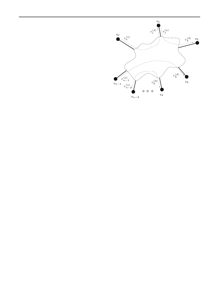
Consider the situation where there are n hosts, or nodes,

and node

v

0

is initially infected with the worm. For each

node

v, let r

(u)

v

and r

(d)

v

denote

v’s up-link and down-link

bandwidths, respectively. When r

(u)

v

= r

(d)

v

, let r

v

denote

this common value. The maximum effective bandwidth from
node

v to node w is then min{r

(u)

v

, r

(d)

w

}. Figure

1

roughly

illustrates communications under our model.

The capacity of the network core is assumed to be

sufficiently large so that nodes can communicate with each
other simultaneously up to their available bandwidths. This
assumption is justified by several facts: (1) our worm does
not generate scanning traffic, which significantly reduces
the traffic intensity as a later simulation shows, (2) the total
amount of traffic sent by the worm is relatively small com-
pared to the Internet core’s capacity, whereas the Internet
backbone is often lightly loaded (around 15% to 25% on
average) due to over-provisioning [

18

], (3) one aim of this

paper is to design effective worms operating on a vulnera-
bility population with moderate bandwidths (e.g., 1 Mbps),
and last but not least (4) when some of the worm’s packets

Backbone Network

Fig. 1 A simple analytical model

are lost due to congestion, our resilient propagation topology
helps alleviate the problem.

Let L

vw

denote the propagation delay from node

v to

node

w. Let L denote the average delay. The worm size is

denoted by W . This can roughly be understood as the num-
ber of bytes of the worm’s machine code. A somewhat subtle
point to notice is that sophisticated propagation mechanisms
might increase W . Most often, though, W should be a con-
stant independent of n. Beside the actual code of size W , the
worm must also transmit a fixed number of a bytes per tar-
get. Each of these “blocks” of a bytes contains the IP address
of the target, and perhaps additional information about the
target such as bandwidth.

Lastly, let p be the probability that a randomly chosen

target is not infectable due to wrong IP-address, software
patched, target down, or firewalled, etc.

2.2 Infection topology

Consider a typical worm infection scenario. Starting from

v

0

,

which keeps a list of addresses and perhaps other informa-
tion about the targets (bandwidths, delays), the worm selects
a subset S of targets to infect. Each node

v in S is also del-

egated set S

v

of targets for

v to infect on its own. Upon

receiving S

v

, node

v can start infecting nodes in S

v

using the

same algorithm. In the mean time,

v

0

and other nodes in S

which were infected before

v can also start their infection

simultaneously.

We can use a directed acyclic graph (DAG) G

= (V, E)

to model this process. The vertex set V consists of all nodes,
including

v

0

, which is called the root or the source. There is

an edge from

v to w if v (after infected) is supposed to infect

w. Since we do not need to infect nodes circularly, a DAG

123

312

D. T. Ha, H. Q. Ngo

is sufficient to model the infection choices. We refer to this
DAG as the infection topology.

For each node

v in G, the set S

v

given to

v by a parent

w is precisely the set of all nodes reachable from v via a
directed path in G. (Note that, for distinct nodes u and

v, S

u

and S

v

might be overlapping if we introduce redundancy to

cope with infection failures.) In order to give

v its list, the

parent

w must know how to effectively compute (in the piece

of code W ) the subgraph of G which consists of all nodes that
can be reached from

w. In practice, this can be done in two

different ways. One is to let the root pre-compute the entire
infection topology for all nodes in the topology at the cost
of transmitting extra topological information for sub-nodes.
Another option is to let the worm instance at

w computes

its own infection sub-topology. The tradeoff, however, is the
CPU consumption at the infected hosts and the reduction
of propagation speed. Depending on his or her priority, the
attacker may choose to employ any of these methods.

2.3 A remark on topology overlay

In order to increase resiliency, a sensible strategy is to use
multiple, say m independent DAGs, for which nodes closer to
the source in one DAG is farther from the source in the other
DAGs. This way, if a part of a DAG got “pruned” by fail-
ures to infect some nodes close to the source, then with high
probability the pruned nodes will be infected via infection
paths in the other DAGs. Indeed, [

21

] used this strategy with

m independent m-ary trees. Basically, this strategy sends out
m instances of the worm based on the same DAG topology
with different rearrangements of vertices. The resiliency is
increased at the cost of a (roughly) linear increase in trans-
mission time.

In this paper, we will focus on constructing one DAG

which is both time-efficient and resilient. The DAG can then
be used as a component in the “overlay” of m DAGs as
described above.

2.4 Infection schedule

It is not sufficient for nodes to make infection decisions based
on the infection topology alone. The second crucial decision
for a node

v to make is to come up with an infection schedule

to infect its children in the topology, i.e. the order in which the
children are to be infected. A schedule is non-preemptive if
the children are to be infected sequentially, one after another,
using the maximum possible bandwidth. A schedule is pre-
emptive if transmissions to different children are overlapping
in time.

Preemptive schedules make estimating the total infection

time quite difficult. Fortunately, in the case of uniform band-
widths and UDP worms, we do not need to consider pre-
emptive schedules as the following Theorem

1

shows. The

theorem helps simplify some later analyses (we will discuss
the uniform bandwidth restriction in the next section).

Theorem 1 Suppose all bandwidths are equal to r and all
links have uniform latency L. With UDP worms, for every
preemptive schedule from a node to a set of children nodes,
there is a non-preemptive schedule in which every target is
infected at time no later than that in the preemptive schedule.

Proof Consider any node

w that starts to infect m targets, say

v

1

, . . . , v

m

, at time 0 following any preemptive schedule. For

each target

v

i

, let T

i

be the time

w finishes the transmission

to

v

i

in the preemptive schedule. Also, let W

i

be the amount

of data transmitted to

v

i

. Without loss of generality, suppose

T

1

≤ T

2

≤ · · · ≤ T

m

. The time at which

v

i

is infected

is T

i

+ L. Let f

i

(t) be the amount of instantaneous band-

width used for the transmission to

v

i

at time t. We then have

W

i

=

T

i

0

f

i

(t)dt, and

m

j

=1

f

j

(t) ≤ r.

Consider the non-preemptive schedule following the same

order 1

, 2, . . . , m, in which w infects one node at a time using

the whole bandwidth capacity. For 1

≤ i ≤ m, let T

i

be the

amount of time until

w completes the transmission to v

i

,

following the non-preemptive schedule. The total amount of
time until

v

i

is infected is T

i

+ L.

To finish the proof, we want to show that T

i

+ L ≤ T

i

+ L,

or simply T

i

≤ T

i

, ∀i. Setting T

0

= 0, we have

T

i

=

i

j

=1

W

j

r

=

i

j

=1

T

j

0

f

j

(t)dt

r

=

i

j

=1

T

j

T

j

−1

(

i
k

= j

f

k

(t))dt

r

≤

i

j

=1

T

j

T

j

−1

r dt

r

= T

1

+ (T

2

− T

1

) + · · · + (T

i

− T

i

−1

) = T

i

2.5 Optimization problems

Total infection time is the total amount of time during which
some worm traffic is still present in the network. The worm
aims to infect the largest number of nodes in the fastest pos-
sible time. There is an intrinsic tradeoff between these two
objectives. The two problems defined below correspond to
optimizing one objective while keeping the other as a thresh-
old constraint. For example, we may want to minimize the
infection time given that at least 90% of infectable targets are
infected; or we may want to maximize the expected number
of infected targets within 5 seconds.

Problem 1 (Minimum Time Malicious Propagation—
mtmp) Given a lowerbound on the expected number of
infected nodes, find an infection topology and the corre-
sponding schedules minimizing the expected infection time.

Problem 2 (Maximum Expansion Malicious Propaga-
tion—

memp) Given an upperbound on the expected infection

123

On the trade-off between speed and resiliency of Flash worms and similar malcodes

313

time, find an infection topology and the corresponding sched-
ules maximizing the expected number of infected nodes.

This paper focuses on the first problem, leaving the sec-

ond problem for future research. The analytical model is quite
simple, yet

mtmp is already NP-hard.

Theorem 2 When the latencies L

wv

are not uniform,

mtmp

is NP-hard even for p

= 0.

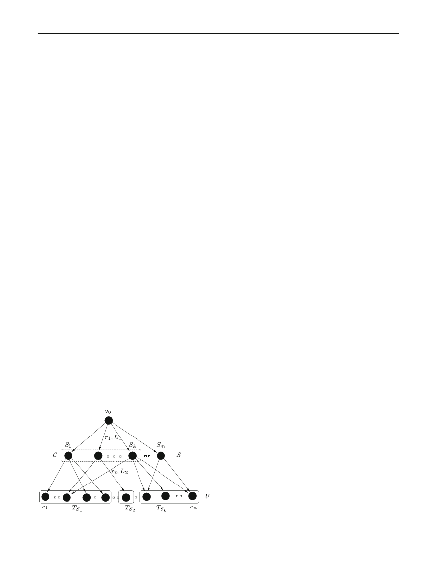
Proof We reduce

Set Cover to mtmp. Consider an instance

of the decision version of

Set Cover where we are given a

collection

S of m subsets of a finite universe U of n elements,

and a positive integer k

≤ m. It is NP-hard to decide if there

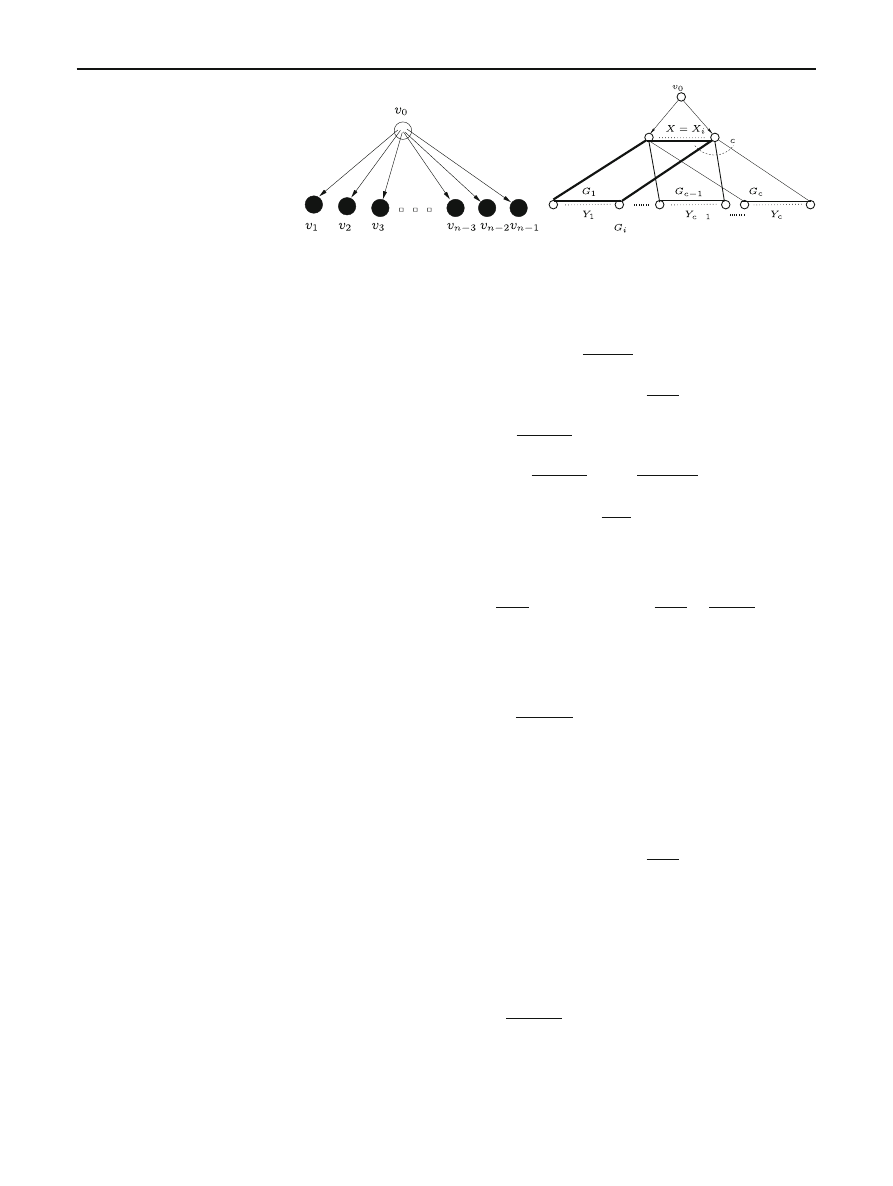
is a set cover of size at most k (Fig.

2

).

An instance of

mtmp is constructed as follows. Set a =

W

= c, where c is an arbitrary integer as long as lg c is a

polynomial in m and n, so that c can be computed in polyno-
mial time. The set of targets is V

= {v

0

}∪S ∪U, where v

0

is

the source. The basic idea is to create a setting where any sat-
isfying propagation topology can only start from

v

0

through

the nodes in

S to the nodes in U. The up- and down-link

bandwidths are as follows.

r

v

0

= r

(d)

S

= r

1

:= c, ∀S ∈ S

r

(u)

S

= r

e

= r

2

:= 2nc, ∀S ∈ S, ∀e ∈ U.

(Recall that, for any node

v ∈ V , r

v

= r means r

(u)

v

= r

(d)

v

=

r .) The latencies are:

L

v

0

S

= L

1

:= 1, ∀S ∈ S

L

Se

= L

2

:= m − k, ∀S ∈ S, ∀e ∈ S

L

vw

= L := m + n + 2. for all other pairs of nodes (v, w).

To complete the proof, we will show that the

Set Cover

instance has a set cover of size at most k if and only if the
mtmp instance constructed above has a propagation topology
and schedule with total infection time at most

(m +n +3/2).

For the forward direction, suppose there is a sub-collec-

tion

C ⊆ S of at most k members such that ∪

S

∈

C

= U. Since

Fig. 2 Reduction from Set Cover to MTMP

C is a set cover, we can choose arbitrarily for each member

S

∈ C a subset T

S

⊂ S such that

S

∈

C

T

S

= U and the

T

S

are all disjoint. (This can be done with a straightforward

greedy procedure.)

Consider the propagation topology G

= (V, E) defined

as follows. The root

v

0

will infect all nodes in

S, i.e. (v

0

, S) ∈

E, for all S

∈ S. Each node S in the cover C infects the nodes

e

∈ T

S

, namely

(S, e) ∈ E, for all S ∈ C and e ∈ T

S

. Now, the

transmission schedule for the root

v

0

is such that

v

0

infects all

nodes in

C first in any order, and then all other nodes in S −C.

Then, for each S

∈ C, S infects nodes in T

S

in any order. The

time it takes for the last node in

S to be infected is T

1

= (na+

mW

)/r

1

+ L

1

= n +m +1. The last node S in C will receive

the worm W and its data (for nodes in T

S

) at time at most

(na + kW)/r

1

+ L

1

= n + k + 1. Up on receiving the worm,

each node S

∈ C will infect nodes in T

S

, which takes time at

most

|T

S

|W/r

2

+L

2

≤ nW/r

2

+L

2

= 1/2+m−k. Because

these infections happen as soon as each node S receives its
worm, the last node in U receiving the worm at time at most
T

2

= (n + k + 1) + (1/2 + m − k) = m + n + 3/2. Thus, the

total infection time is at most max

{T

1

, T

2

} = m + n + 3/2,

as desired.

Conversely, suppose there is a propagation topology G

=

(V, E) and some transmission scheduling such that the total
infection time is at most m

+ n + 3/2. Note that (v

0

, e) /∈ E

for all e

∈ U, because the latency L

v

0

,e

is m

+ n + 2 >

m

+ n + 3/2. For the same reason, (S

1

, S

2

) /∈ E for any

S

1

, S

2

∈ S; (e, S) /∈ E for any e ∈ U and S ∈ S; and

if e

/∈ S, then (S, e) /∈ E. Consequently, the only possible

edges of G are of the form

(v

0

, S) for S ∈ S, and (S, e) for

e

∈ S.

Now, let T

S

= {e | (S, e) ∈ E} be the set of out-neighbors

of S in G. Let

C = {S | T

S

= ∅} be the set of S with non-zero

out-degrees. It is clear that

C is a set cover of the original Set

Cover instance, otherwise not all nodes in U are infected.
We show that

C has at most k members. Suppose C has at

least k

+ 1 members, then the last member S of C receiving

the worm at time at least T

1

= (na + (k + 1)W)/r

1

+ L

1

=

n

+ k + 2. This last member will have to infect nodes in T

S

(there is at least one node in this set), which takes time at least
T

2

= W/r

2

+ L

2

= 1/(2n)+m −k > m −k. Consequently,

the total infection time is at least T

1

+ T

2

> n + m + 3/2.

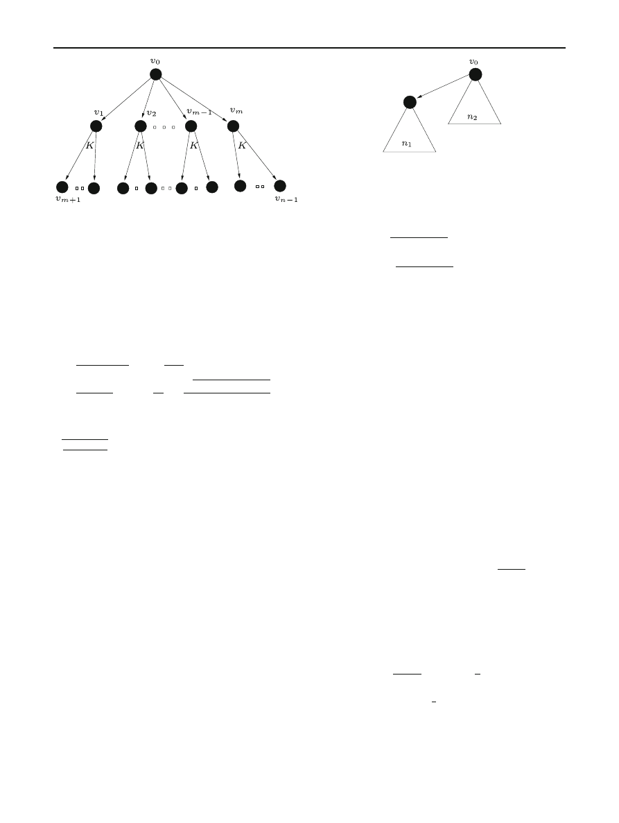
2.6 An example

Next, let us revisit the infection scheme of the non-resilient
UDP Flash Worm presented in Section 2 of [

21

] to illustrate

the model discussed above. Figure

3

depicts the infection

topology of this scheme, which is a tree whose root is the
source

v

0

. The source first infects m intermediate nodes (from

v

1

to

v

m

), each of which continues to infect K other nodes.

The infection schedule was not provided in the original paper.

123

314

D. T. Ha, H. Q. Ngo

Fig. 3 Infection topology of a Flash worm in [

21

]

For simplicity, we assume all nodes have the same up-

and down-link bandwidths of r . Thanks to Theorem

1

, we

can assume a parent node infects its children in any sequen-
tial order. Finally, as in [

21

], the pairwise latencies are all

the same, denoted by L. Noting that n

= m(K + 1) + 1, the

propagation time for this topology is

t

1

=

m

(W + aK )

r

+ L +

K W

r

+ L

(1)

≥

(n − 1)a

r

+ 2L −

W

r

+ 2

√

W

(W − a)(n − 1)

r

The lower bound can be attained by setting K

=

(n−1)(W−a)

W

− 1.

3 An even faster flash worm

When the latencies are not uniform, the general

mtmp prob-

lem is NP-hard by Theorem

2

. This result justifies a further

refinement of the model where we use the average bandwidth
r as up- and down-link bandwidth, and the average latency

L as the pair-wise latency. This section demonstrates that

this simpler model already allows us to design a faster Flash
worm which requires much less bandwidth at the source.

We focus on minimizing the infection time assuming no

infection failure, deferring the failure-prone case to Sect.

5

.

In this case, any topology in which all targets are reachable
from the root would infect the entire population. Moreover,
each node needs to be infected only once, implying that a tree
is sufficient. Thanks to Theorem

1

, we only need to consider

non-preemptive schedules.

Suppose the source first infects the root of a sub-tree of

size n

1

(see Fig.

4

). The tree on n nodes can be viewed as a

combination of two sub-trees of size n

1

and n

2

= n − n

1

.

first target

Fig. 4 The Recursive Tree topology, p

= 0 case

Let T

(n) be the minimum infection time for n nodes. Then

T

(n) can be recursively computed:

T

(n) = min

n

1

≤n−1

W

+a(n

1

−1)

r

+max{T (n

1

)+L, T (n

2

)}

= min

n

1

≤n/2

W

+a(n

1

−1)

r

+max{T (n

1

)+L, T (n

2

)}

(2)

T

(n) can be computed in O(n

2

)-time. A newly infected node

v does not need to recompute the value n

1

for its sub-tree (of

size

|S

v

|). The optimal choices of n

1

for different values of

n can be pre-computed and then be transmitted along with
the address list. This strategy adds a fixed number of bytes
(

≤ 4) to be transmitted per target, and thus can be included

in the block of a bytes per target.

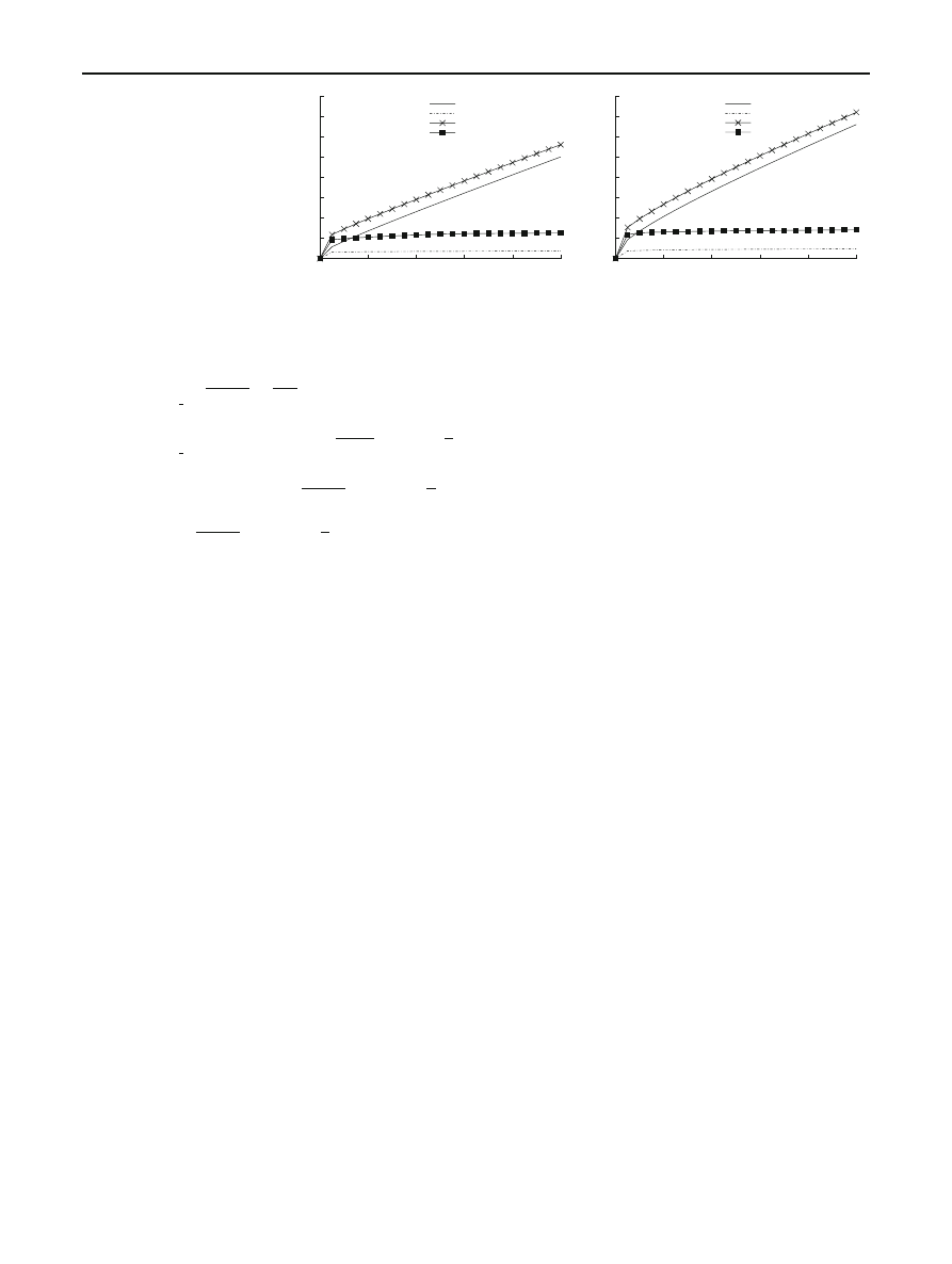
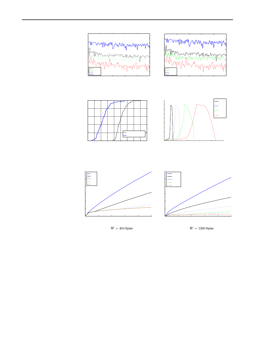
Figure

5

(a, b) compares the infection time of this recursive

tree topology with the Flash Worm topology as the popula-
tion size varies. Two values for W are observed—404 and
1,200 bytes—corresponding to actual sizes of Slammer and
Witty [

1

,

2

]. As seen in the figure, our worm infection time

scales very well with the population size. Our topology per-
forms better as L decreases. The time difference between the
two topologies is reduced as L increases. When L is large,
the optimal tree based on (

2

) becomes shallower, thus per-

forms more like the Flash Worm topology. Intuitively, when
the propagation time is too large the source can actually send
all worm packets to all targets within the propagation delay
of the first packet. The trend can be explained with a sim-
ple analysis. At one extreme, when L

>

W

(n−1)

r

equation

(

2

) sets n

1

= 1 for any n, yielding a star topology. At the

other extreme, when L

= 0 or very close to zero, the opti-

mal topology is a binomial tree, as shown by the following
proposition.

Proposition 3 When L

→ 0, we have

T

(n) = log n

W

− a

r

+ (n − 1)

a

r

(3)

which is attained at n

1

=

n
2

.

Proof We show this by induction. When n

= 1, T (1) = 0

since the source is already infected. Suppose (

3

) holds for all

123

On the trade-off between speed and resiliency of Flash worms and similar malcodes

315

Fig. 5 Analytical infection
time of Flash Worm and
recursive tree topologies with
varying n. a L

=100, 400ms,

W

=404 Bytes. b L=100,

400 ms, W

=1,200 Bytes

0

1

2

3

4

5

6

7

8

0

200000

400000

600000

800000

1e+06

Time (seconds)

Number of nodes

Flash Worm topo.,L=100
Recursive Tree,L=100
Flash Worm topo.,L=400
Recursive Tree,L=400

1

2

3

4

5

6

7

8

0

0

200000

400000

600000

800000

1e+06

Time (seconds)

Number of nodes

Flash Worm topo.,L=100
Recursive Tree,L=100
Flash Worm topo.,L=400
Recursive Tree,L=400

L = 100ms, 400 ms,W = 404 Bytes

L = 100 ms, 400 ms, W = 1200 Bytes

(a)

(b)

n

≤ k − 1. For n = k, we have

T

(k) = min

1

≤n

1

≤

k
2

W

− a

r

+

an

1

r

+ T (k − n

1

)

= min

1

≤n

1

≤

k
2

(1+log(k−n

1

))

W

−a

r

+(k−1)

a

r

= (1 + log(k − k/2))

W

− a

r

+ (k − 1)

a

r

= log k

W

− a

r

+ (k − 1)

a

r

.

This value is achieved at n

1

= n/2.

4 Simulation

To cope with the obstacle of NP-hardness, we refined our
analytical model by assuming uniform bandwidths and laten-
cies. Does the above analytical comparison result holds in
practice? In the bandwidth case, if the uniform bandwidth is
taken to be a lowerbound of all actual bandwidths, then the
analytical infection time computed from the model is a worst-
case infection time bound. The uniform latency assumption,
however, might be too strong.

To address this doubt, we simulated the propagation of

the worms in a network with varied latencies. These laten-
cies were generated in accordance with the empirical latency
distribution in the Skitter data set [

7

]. We generated 100 sets

of latencies, corresponding to 100 network configurations.

For each network configuration, we computed the recur-

sive topology based on (

2

), setting L equal to the average

Internet latency, which is about 201 ms. Due to enormous
time consumption, we were only able to run the simulation
with n

= 100,000 nodes instead of 1 million nodes. We

kept r

= 1 Mbps as before. We then simulated and com-

pare the Flash Worm and the Recursive Tree topologies on
the same network. Figure

6

a plots the ratio of the simulated

infection time of the Flash Worm topology over that of the
Recursive Tree topology over 100 simulations with several
values of latency variances. Firstly, it can be seen that the

time-improvement ratio is roughly close to that of the same
analytical data point (at n

= 100, 000) shown in Fig.

5

. Sec-

ondly, as expected the smaller the latency variance, the better
the time-improvement ratio. This means that our worm will
work well if the target population does not have many large
clusters of near-by nodes.

Furthermore, to see the effect of the latency variance,

Fig.

6

b shows the difference between the analytical time-

improvement ratio and the simulation time-improvement
ratio. The analytical time-improvement ratio is a slight over-
estimate for small variances, and gets worse as the variance
increases. However, it is still well within a small constant
times the real time-improvement ratio.

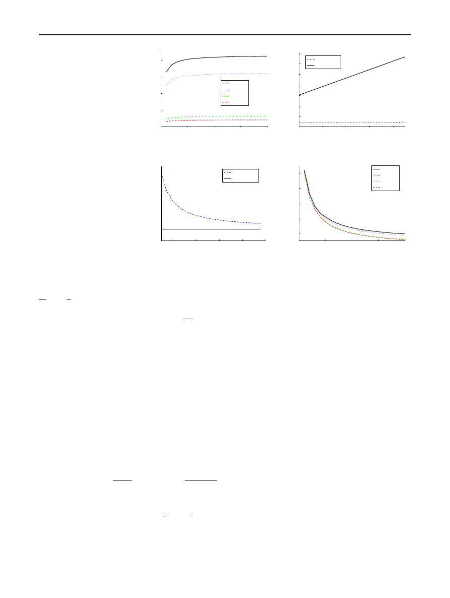
We also simulated the worm traffic generated during the

propagation process. Figure

6

d summarizes the total traffic

for the recursive topology with 4 average values of L. For
this simulation, we set n

= 1 million nodes. As can be seen

from the figure, the total traffic has a peak value of 400 Mbps,
independent of the latencies.

For this amount of total traffic the worm is less likely to

cause any significant instability in the network core (com-
pared to scanning worms), validating our assumption for the
analytical model.

Another advantage of the recursive topology is that it can

retain similar time efficiency as the Flash Worm of [

21

] even

when starting from a root node with much less bandwidth
capacity. Figure

7

(a, b) shows the minimum bandwidth at

the root of the Flash Worm in [

21

] required in order for the

Flash worm to propagate as fast as our worm, whose starting
node has only 1 Mbps capacity. The figures plot this required
root’s bandwidth as a function of the total number of nodes
n for two empirical values of W . We also varied L to see the
effect of latencies on the efficiency of the Flash worm and
our worm.

As can be seen, the result is consistent with our previ-

ous analysis. The required root’s bandwidth for Flash worms
stays at peak for small values of L and reduces gradually as L
increases. In particular, at L

= 0.1s, the Flash worm needs a

significantly larger bandwidth of 60 Mbps (compared to the
uniform bandwidth 1 Mbps using our recursive topology).

123

316

D. T. Ha, H. Q. Ngo

Fig. 6 The performance of
Flash Worm and Recursive Tree
topologies with n

= 100,000.

a Infection time of Flash worm
in [21] over our worm (time
improvement ratio).
b Difference between simulated
and analytical time improvement
ratios. c Cumulative
distributions. d Traffic during
propagation, 1M hosts

0

20

40

60

80

100

0.9

1

1.1

1.2

1.3

1.4

1.5

1.6

1.7

1.8

Run

Simulated Propagation Time Ratio Between Flash

Worm And Recursive Topology

STD=72
STD=52
STD=32
STD=12

0

20

40

60

80

100

−0.9

−0.8

−0.7

−0.6

−0.5

−0.4

−0.3

−0.2

−0.1

Run

Difference Between Simulated And Estimated Propagation

Time Ratio (Flash Worm/Recursive Topology)

STD=72
STD=52
STD=32
STD=12

1.1

1.2

1.3

1.4

1.5

1.6

1.7

1.8

1.9

0

0.2

0.4

0.6

0.8

1

Time (seconds)

F(x)

CDF (100 Runs)

Flash Worm Topo.

Recursive Topology

0

0.5

1

1.5

2

2.5

0

0.5

1

1.5

2

2.5

3

3.5

4

4.5

x 10

8

Time (seconds)

Traffic (bytes)

L=0.1

L=0.2

L=0.4

L=0.8

Infection time of Flash worm in [21]
over our worm (time improvement ratio)

(a)

Cumulative distributions

(c)

Traffic during propagation,1M hosts

(d)

Difference between simulated and analytical
time improvement ratios

(b)

Fig. 7 Minimum source
bandwidth for the Flash Worm
topology to achieve the same
effect as our worm. a W

= 404

bytes. b W

= 1,200 bytes

0

2

4

6

8

10

x 10

5

0

1

2

3

4

5

6

x 10

7

W(byte) = 404.000000

Number of Susceptible Nodes

Equivalent Bandwidth (bps)

L=0.1
L=0.2
L=0.4
L=0.8
L=1.6

0

2

4

6

8

10

x 10

5

0

2

4

6

8

10

12

x 10

7

W(byte) = 1200.000000

Number of Susceptible Nodes

Equivalent Bandwidth (bps)

L=0.1
L=0.2
L=0.4
L=0.8
L=1.6

(a)

(b)

This number even grows to more than 100 Mbps when W
increases, as shown in Fig.

7

b.

5 The tradeoff between speed and resiliency

For each infection topology G, let N

(G) and T (G) be the

expected number of infected nodes and the expected total
infection time, respectively. For any particular G, increasing

N

(G) forces T (G) to increase also. This is the tradeoff we

investigate. Define

N

(n)=max{N(G) | G is an infection topology on n nodes},

T

(n)=min{T (G) | G is an infection topology on n nodes}.

We first identify the topology with the largest expected num-
ber of infected nodes in the following lemma.

Lemma 4 Let S be a star on n nodes rooted at

v

0

. Then, S is

the topology which maximizes N

(G). In particular, N(S) =

N

(n) = 1 + (n − 1)(1 − p).

Proof Consider an arbitrary infection topology G. For each
node

v

i

(0

≤ i ≤ n − 1), where v

0

is the source, let Z

i

be the

random variable indicating if

v

i

is infected using this topol-

ogy. Then, clearly Prob

[Z

i

= 1] ≤ 1 − p. Thus, by linearity

of expectation,

123

On the trade-off between speed and resiliency of Flash worms and similar malcodes

317

Fig. 8 Resilient Topologies.
a Most resilient topology S.
b The Resilient Topology R

copies

The

are all copies of the same graph

H

−

Most resilient topology

S

The resilient topology

R

(a)

(b)

N

(G) = E

n

−1

i

=0

Z

i

=

n

−1

i

=0

E

[Z

i

]

= 1 +

n

−1

i

=1

E

[Z

i

] ≤ 1 + (n − 1)(1 − p)

(4)

Equality holds if and only if Prob

[Z

i

= 1] = 1 − p, which

means that there is a direct edge from

v

0

to

v

i

. Otherwise,

there is a positive probability that every path from the root to
v

i

has a node not infectable, implying

v

i

not infectable.

Knowing the maximum expectation N

(n), we can use it as

a benchmark to characterize the tradeoff between N

(G) and

T

(G) for any infection topology G. Note that, while N(S)

is optimal T

(S) = (n − 1)W/r + L is not. A natural prob-

lem is to find a topology G for which N

(G) is very close to

the optimal N

(S), say more than a factor f of N(S), while

T

(G) is much smaller than T (S). An obvious strategy is to

choose any subset of n

< n nodes and apply topology S on

n

nodes, where n

≈ f n. This way, the sacrifice in N(n) is

linear and the payoff in T

(n) is also linear. Fortunately, there

is a much better strategy than this simple-minded approach.
We will show that, to achieve a linear payoff in T

(G), we can

still keep N

(G) exponentially close to optimal! The result,

in a sense, is the best one can hope for. (The converse is also
desirable, where a linear sacrifice in N

(G) gives an expo-

nential payoff in T

(G). This problem is open!)

Our infection topology named the resilient topology R

is illustrated in Fig.

8

b. For i

= 1, . . . , c, let G

i

= (X

i

∪

Y

i

; E

i

) be copies of the same bipartite graphs H. (H to be

specified.) To construct R, we “glue” together the X

i

-side of

G

1

, . . . , G

c

, i.e. identify vertices in the X

i

in any one-to-one

manner. Let X denote the glued X

i

, and Y

= Y

1

∪ · · · ∪ Y

c

.

The source

v

0

has an edge to each vertex in X . In total, the

vertex set of R is

{v

0

} ∪ X ∪ Y . Different choices of the

“seed component” H lead to different degrees of resiliency,
as explained in the following lemma and theorems.

In the following lemma, we consider a very simple case

to illustrate the idea and the complexity of analyzing the
expected infection time.

Lemma 5 Let H (i.e. the G

i

) be any k-regular simple bipar-

tite graph. Let l

=

kc

+Lr/W

kca

/W+1

, we have

N

(R) = (n − 1)(1 − p)

1

−

c

1

+ c

p

k

+ 1.

(5)

T

(R) =

W

+ kca

r

x

(1 − p

l

+ p

2l

)

+ Lp

l

+

W

+ kca

r

l p

l

+

p

(p

l

− 1)

1

− p

(1 − p

l

)

+ (1 − p

l

)

2

kcW

r

+ 2L

.

(6)

In particular, the following limit and theorem follows imme-
diately.

lim

n

→∞

T

(R)

T

(S)

= (1 − p

l

+ p

2l

)

1

1

+ c

+

kca

/W

1

+ c

.

(7)

Theorem 6 For sufficiently large n, topology R has the
expected number of infected nodes exponentially close to
optimality, yet reduces the expected infection time by a linear
factor of

1

+c(ka/W)

1

+c

.

Proof (of Lemma

5

)

Denote x

= |X| and y = |Y |. Using the fact that x + y =

n

− 1 and linearity of expectation again, we can easily com-

pute:

N

(R) = 1 + x(1 − p) + y(1 − p)(1 − p

k

)

= (n − 1)(1 − p)

1

−

c

1

+ c

p

k

+ 1

(8)

Computing the expected time T

(R) is significantly more

complicated. Firstly, recall that infection time is the amount
of time starting from when the source sends out its first bit
until the last bit of the worm is gone from the network. Thus,
the time it takes until the last packet from the source to the
nodes in X completely disappears from the network is

Z

1

= x

W

+ kca

r

+ L.

Secondly, let x

I

be the last node in X which is infected. Note

that, I is a random variable taking values from 0 to x, where

123

318

D. T. Ha, H. Q. Ngo

the value of 0 indicates that no node in X is infected. It fol-
lows that

Prob

[I ≤ j] = p

x

+

j

i

=1

(1 − p)p

x

−i

= p

x

− j

(9)

Prob

[I > j] = 1 − p

x

− j

(10)

If I

> 0, the total amount of time until the last bit from x

I

disappears from the network is

Z

2

= I

W

+ kca

r

+ L +

kcW

r

+ L

= I

W

+ kca

r

+

kcW

r

+ 2L

If I

= 0, set Z

2

= 0. Depending on the relationship between

various parameters (k

, L, . . .), the source might still be trans-

mitting when x

I

has finished, or vice versa. The total time the

worm is on the network is Z

= max{Z

1

, Z

2

}, where Z

1

is a

constant while Z

2

is a random variable. We wish to compute

T

(R) = E[Z] = Z

1

Prob

[Z

1

≥ Z

2

]

+E[Z

2

| Z

1

< Z

2

] Prob[Z

1

< Z

2

].

(11)

Note that Z

1

≥ Z

2

is equivalent to I

≤ x −

kc

+Lr/W

kca

/W+1

.

Assuming n is large, then x is greater than the constant l

=

kc

+Lr/W

kca

/W+1

. From (

9

) and (

10

), we have Prob

[Z

1

≥ Z

2

] =

p

l

, and Prob

[Z

1

< Z

2

] = 1 − p

l

. It remains to compute

E

[Z

2

|Z

1

< Z

2

]. Since Z

1

< Z

2

is equivalent to I

> x − l,

we have

E

[Z

2

|Z

1

< Z

2

] =

x

j

=x−l+1

E

[Z

2

| I = j] Prob[I = j]

=

x

j

=x−l+1

j

W

+ kca

r

+

kcW

r

+ 2L

(1 − p)p

x

− j

=

W

+ kca

r

x

(1 − p

l

) + lp

l

+

p

(p

l

− 1)

1

− p

+ (1 − p

l

)

kcW

r

+ 2L

Combined with (

11

), we get

T

(R) =

W

+ kca

r

x

(1 − p

l

+ p

2l

)

+

W

+ kca

r

l p

l

+

p

(p

l

− 1)

1

− p

(1 − p

l

)

+Lp

l

+ (1 − p

l

)

2

kcW

r

+ 2L

.

(12)

We next illustrate how this theorem can be applied. To

reduce the infection time for this topology, we want the limit
(

7

) to be as small as possible, subject to some desired thresh-

old in terms of the expected number of infected nodes. For

instance, to guarantee that N

(R) ≥ f N(n), we choose k and

c to minimize the limit (

7

), subject to the condition that

(n−1)(1− p)

1

−

c

c

+ 1

p

k

+1 ≥ f [(n−1)(1− p)+1],

which is equivalent to

k

≥

− ln

(1 − f )(c + 1)/c(

1

(n−1)(1−p)

+ 1)

ln

(1/p)

(13)

This can be done in a variety of ways, one of which is to
choose a relatively large c (thus reducing the infection time),
then choose k to satisfy constraint (

13

). This lower bound for

k is relatively small. For most values of c the lower bound
for k is at most 4, even when f is large (90% or more). When

p is large, the lower bound becomes trivial, as can be seen

from Fig.

9

a.

As mentioned earlier, to infect f n nodes, one can also

select n

≈ f n nodes and apply topology S on these nodes.

However, this approach is very inefficient compared to using
topology R. Figure

9

b depicts the gap between the expected

propagation time using two topologies, as f varies. Topology

R is shown to be more efficient, especially when the desired

ratio f is large.

The limit (

7

) tells us roughly how far away from T

(S) our

infection time is. The limit ratio is simpler to work with than
the actual ratio, which is dependent on n. Moreover, when n
is in the order of tens of thousands, the limit ratio accurately
depicts the actual ratio as shown in Fig.

9

c. This limit also

does not depend very much on the value of p, but more on
the value of c. In fact, Fig.

9

d shows that the limit becomes

independent of small values of p.

A stronger notion of resiliency
While N

(R) within a fraction f of the optimal is a good

notion of resiliency (the same notion as that in [

21

]), it is still

a weak guarantee in the following sense. The ratio between

N

(R)/N(n) is large when the expectation N(R) is large. This

expectation is a weighted-average in accordance with the fail-
ure distribution of the targets imposed by p. This means that
many node failure combinations still yield a smaller num-
ber of infected nodes than N

(R). It would be nice to have a

stronger guarantee than that.

In what follows, we will show that, with the right choice

of H , for any given

> 0 the number of infected nodes is

within a fraction

(1 − ) of the number of infectable nodes

with probability exponentially close to 1.

A

(w, )-extractor is a bipartite graph H = (L ∪ R, E)

with left part

|L| = x ≥ w and right part |R| = y, such that

every subset of at least

w left vertices has at least (1 − )y

neighbors on the right. It is known that, for any

and any

w ≤ x, there exist (w, )-extractors in which all left vertices
have degree d

= (log x), y = (wd), and the distri-

123

On the trade-off between speed and resiliency of Flash worms and similar malcodes

319

Fig. 9 Limit and actual
infection time ratios

0

5

10

15

20

0

1

2

3

4

c

Lower bound of k

W = 404 bytes, q = 0.9, p = 0.5, 0.4, 0.1 and 0.001

p=0.5

p=0.4

p=0.1

p=0.001

50

60

70

80

90

50

100

150

200

250

300

350

400

f (%)

Expected Infection Time (s)

W = 404 bytes, c = 5, n=10

6

, p = 0.1

Topology R

Topology S

2

4

6

8

10

x 10

5

0.174

0.175

0.176

0.177

0.178

0.179

0.18

n

Actual Time Ratio

W = 404 bytes, c = 5, q=0.9, p = 0.1

Actual Ratio

R

0

5

10

15

20

0.1

0.2

0.3

0.4

0.5

c

Ratio

W = 404 bytes, q = 0.9, p = 0.5, 0.4, 0.01 and 0.001

p=0.5

p=0.4

p=0.01

p=0.001

Lower bound of k

(a)

Infection time of topology R and S

(b)

Limit Ratio and Actual Ratio gap

(c)

Limit Ratio dependency on p

(d)

bution of right degrees are close to uniform, i.e. of degree

xd

y

= (

x

w

) [

13

].

Theorem 7 Fix any constant

> 0. Let x =

n

−1

c

+1

for any

chosen constant c as before. Let

α > 0 be any constant such

that

α < 1 − p. Set w = αx, and let H be the (w, )-

extractor as described above. Then, with probability at least
1

− exp(−(n)) (i.e. exponentially close to 1), topology R

will be able to infect a

(1 − )-fraction of all nodes that are

infectable.

Proof The important point to notice here is that, by defini-
tion of extractors, if less than a

(1 − )-fraction of nodes in

Y are reachable, then more than x

− w = (1 − α)x nodes in

X are not infected. Let M be the number of uninfected nodes

in X , then, noting that E

[M] = xp and applying Chernoff

bound,

Prob

[less than (1 − )y nodes infected] ≤ Prob[M > αx]

= Prob

M

>

1

+

α − p

p

x p

≤ exp

−

x

(α − p)

2

3 p

Note that, the degree of vertices in Y is

(

x

w

) = (

1

α

), which

is a constant. Hence, the linear time improvement factor over
topology S still holds!

6 Discussions and future work

Similar to the Flash Worm designed in [

21

], the character-

istics of our super fast worm make it a serious challenge
to existing defense systems. For example, the use of hitlist
helps the worm avoid dark-net/dark-port or scanner detec-
tors based on failed attempts to non existing addresses [

10

].

Its propagation speed of seconds renders traditional defense
systems with response time of minutes useless. However,
fast worms in general are not without weaknesses. First, it is
vulnerable at the hitlist creation stage where it can include
some of the honeypots [

3

] in its target list. A honeyfarm

which correlates similarity of captured worm instances can
raise an alert at the beginning of an attack. Similarly, due to
its super fast propagation, the worm will necessarily intro-
duce a traffic spike into the network, disrupting normal traffic
patterns. Thus, it becomes more prone to being detected by
distributed detectors with traffic analysis capability similar
to that of Autograph [

11

]. Finally, a recursive topology like

in Sect.

3

, although optimal in terms of speed, may incor-

porate nodes with high-fanout (at hundreds of connections).
This feature makes the worm vulnerable to host based throt-
tling systems like Williamson’s [

24

]. (Note, however, that if

the worm employs a less aggressive propagation topology
like the resilient one, this is no longer the case. We leave the
investigation of such topology’s performance in practice for
future work).

123

320

D. T. Ha, H. Q. Ngo

On the positive side, our design can be adapted to be used

in defense systems which need to disseminate a message (e.g.
alerts) to distributed locations as fast as possible, especially
those rely on overlay platforms. For example, in Vojnovic’s
automated patching system [

23

], patches can be propagated

from a center server to superhosts (or even from superhosts
to final hosts) following a topology similar to ours. Since our
topology optimizes propagation based on parallel transmis-
sion, we expect it to perform better than normal P2P topolo-
gies not geared towards this goal.

In terms of future research, an open problem is thus to

devise a good approximation algorithm for MTMP, when it
is NP-hard. It is important to also study how current contain-
ment policies such as that in [

17

] can thwart these infection

schemes. Last but not least, the second problem we formu-
lated—

memp—has not been addressed at all.

References

1.

http://www.f-secure.com/v-descs/mssqlm.shtml

2.

http://www.f-secure.com/v-descs/witty.shtml

3.

http://www.honeynet.org

4.

http://www.icir.org/yoid/

5. Arce, I., Levy, E.: An analysis of the slapper worm. IEEE Secur.

Priv. 1, 82–87 (2003)

6. Banerjee, S., Bhattacharjee, B., Kommareddy, C.: Scalable appli-

cation layer multicast. In: SIGCOMM 2002, New York, NY, USA.
ACM Press, pp. 205–217 (2002)

7. CAIDA,

Skitter

datasets.

http://www.caida.org/tools/

measurement/skitter/

8. Chen, Z., Gao, L., Kwiat, K.: Modeling the spread of active worms,

in INFOCOM 2003. Twenty-Second Annual Joint Conference of
the IEEE Computer and Communications Societies. IEEE, vol. 3,
Mar 30–Apr 3 2003, pp. 1890–1900

9. Filiol, E., Franc, E., Gubbioli, A., Moquet, B., Roblot, G.: Com-

binatorial optimisation of worm propagation on an unknown net-
work. Int. J. Comput. Sci. 2, 124–130 (2007)

10. Jung, J., Paxson, V., Berger, A.W., Balakrishnan, H.: Fast portscan

detection using sequential hypothesis testing. In: IEEE Symposium
on Security and Privacy. IEEE Computer Society, pp. 211–225
(2004)

11. Kim H.-A., Karp B. (2004) Autograph: toward automated, distrib-

uted worm signature detection. In: Proceedings of the 13th USE-
NIX Security Symposium, USENIX, August 2004

12. Liljenstam, M., Nicol, D.M., Berk, V.H., Gray, R.S.: Simulating

realistic network worm traffic for worm warning system design
and testing. In: WORM ’03: Proceedings of the 2003 ACM work-
shop on Rapid malcode, New York, NY, USA. ACM Press, New
York, pp. 24–33 (2003)

13. Lu, C.-J., Reingold, O., Vadhan, S., Wigderson, A.: Extractors:

optimal up to constant factors. In: Proceedings of the Thirty-Fifth
Annual ACM Symposium on Theory of Computing, New York.
ACM, New York, pp. 602–611 (2003) (electronic)

14. Moore, D., Paxson, V., Savage, S., Shannon, C., Staniford, S.,

Weaver, N.: Inside the slammer worm. IEEE Secur. Priv. 1, 33–
39 (2003)

15. Moore, D., Paxson, V., Savage, S., Shannon, C., Staniford, S.,

Weaver, N.: The spread of the sapphire/slammer worm. CAIDA,
pp. 33–39 (2003)

16. Moore, D., Shannon, C., Brown, J.: Code-red: a case study on the

spread and victims of an internet worm. In: IMW ’02: Proceedings
of the 2nd ACM SIGCOMM Workshop on Internet measurment,
New York, NY, USA. ACM Press, New York, pp. 273–284 (2002)

17. Moore, D., Shannon, C., Voelker, G., Savage, S.: Internet quar-

antine: requirements for containing self-propagating code. In: IN-
FOCOM 2003. Twenty-Second Annual Joint Conference of the
IEEE Computer and Communications Societies. IEEE, vol. 3, pp.
1901–1910 (2003)

18. Odlyzko, A.: Data networks are lightly utilized, and will stay that

way. Rev. Netw. Econ. 2, 210–237 (2003)

19. Ratnasamy, S., Francis, P., Handley, M., Karp, R., Schenker, S.:

A scalable content-addressable network. In: SIGCOMM 2001, pp.
161–172 (2001)

20. Shannon, C., Moore, D.: The spread of the witty worm. IEEE Secur.

Priv. Mag. 2, 46–50 (2004)

21. Staniford, S., Moore, D., Paxson, V., Weaver, N.: The top speed

of flash worms. In: WORM ’04: Proceedings of the 2004 ACM
workshop on Rapid malcode, New York, NY, USA. ACM Press,
New York, pp. 33–42 (2004)

22. Staniford, S., Paxson, V., Weaver, N.: How to own the internet

in your spare time. In: Proceedings of the 11th USENIX Secu-
rity Symposium, Berkeley, CA, USA. USENIX Association, pp.
149–167 (2002)

23. Vojnovic, M., Ganesh, A.: On the effectiveness of automatic patch-

ing. In: WORM ’05: Proceedings of the 2005 ACM workshop on
Rapid malcode, New York, NY, USA. ACM Press, New York, pp.
41–50 (2005)

24. Williamson, M.M.: Throttling viruses: Restricting propagation to

defeat malicious mobile code. In: ACSAC ’02: Proceedings of the
18th Annual Computer Security Applications Conference, Wash-
ington, DC, USA. IEEE Computer Society, p. 61 (2002)

25. Zou, C.C., Gong, W., Towsley, D.: Code red worm propagation

modeling and analysis. In: CCS ’02: Proceedings of the 9th ACM
conference on Computer and communications security, New York,
NY, USA. ACM Press, New York, pp. 138–147 (2002)

26. Zou, C.C., Gong, W., Towsley, D.: Worm propagation modeling

and analysis under dynamic quarantine defense. In: WORM ’03:
Proceedings of the 2003 ACM workshop on Rapid malcode, New
York, NY, USA. ACM Press, New York, pp. 51–60 (2003)

27. Zou, C.C., Gong, W., Towsley, D., Gao, L.: The monitor-

ing and early detection of internet worms. IEEE/ACM Trans.
Netw. 13, 961–974 (2005)

28. Zou, C.C., Towsley, D., Gong, W., Cai, S.: Routing worm: a fast,

selective attack worm based on ip address information. In: PADS
’05: Proceedings of the 19th Workshop on Principles of Advanced
and Distributed Simulation, Washington, DC, USA. IEEE Com-
puter Society, pp. 199–206 (2005)

123