IEEE TRANSACTIONS ON INDUSTRY APPLICATIONS, VOL. 38, NO. 4, JULY/AUGUST 2002

1087

Sensorless Vector Control of Induction Motors at

Very Low Speed Using a Nonlinear Inverter

Model and Parameter Identification

Joachim Holtz, Fellow, IEEE, and Juntao Quan

Abstract—The performance of vector-controlled induction

motor drives without speed sensor is generally poor at very
low speed. The reasons are offset and drift components in the
acquired feedback signals, voltage distortions caused by the non-
linear behavior of the switching converter, and the increased
sensitivity against model parameter mismatch. New modeling
and identification techniques are proposed to overcome these
problems. A pure integrator is employed for stator flux estima-
tion which permits high-estimation bandwidth. Compensation
of the drift components is done by offset identification. The
nonlinear voltage distortions are corrected by a self-adjusting
inverter model. A further improvement is a novel method for on-
line adaptation of the stator resistance. Experiments demonstrate
smooth steady-state operation and high dynamic performance
at extremely low speed.

Index Terms—Induction motor, low-speed operation, parameter

identification, sensorless control, vector control.

I. I

NTRODUCTION

C

ONTROLLED induction motor drives without speed
sensor have developed as a mature technology in the

past few years. However, their performance at very low speed
is poor. The main reasons are the limited accuracy of stator
voltage acquisition, the presence of offset and drift compo-
nents in the acquired voltage signals, their limited bandwidth,
offsets and unbalances in the current signals, and the increased
sensitivity against model parameter mismatch.

These deficiencies degrade the accuracy of flux estimation at

low speed. The dynamic performance of a sensorless drive then
deteriorates. Sustained operation at very low speed becomes im-
possible as ripple components appear in the machine torque and
the speed starts oscillating, eventually leading to instable oper-
ation of the system.

Paper IPCSD 02–025, presented at the 2001 Industry Applications Society

Annual Meeting, Chicago, IL, September 30–October 5, and approved for
publication in the IEEE T

RANSACTIONS ON

I

NDUSTRY

A

PPLICATIONS

by the

Industrial Drives Committee of the IEEE Industry Applications Society.
Manuscript submitted for review October 15, 2001 and released for publication
May 10, 2002.

J. Holtz is with the Electrical Machines and Drives Group, University of Wup-

pertal, 42097 Wuppertal, Germany (e-mail: [e-mail]).

J. Quan is with the Danaher Motion Group, Kollmorgen-Seidel, Duesseldorf,

Germany (e-mail: [e-mail]).

Publisher Item Identifier 10.1109/TIA.2002.800779.

II. S

OURCES OF

I

NACCURACY AND

I

NSTABILITY

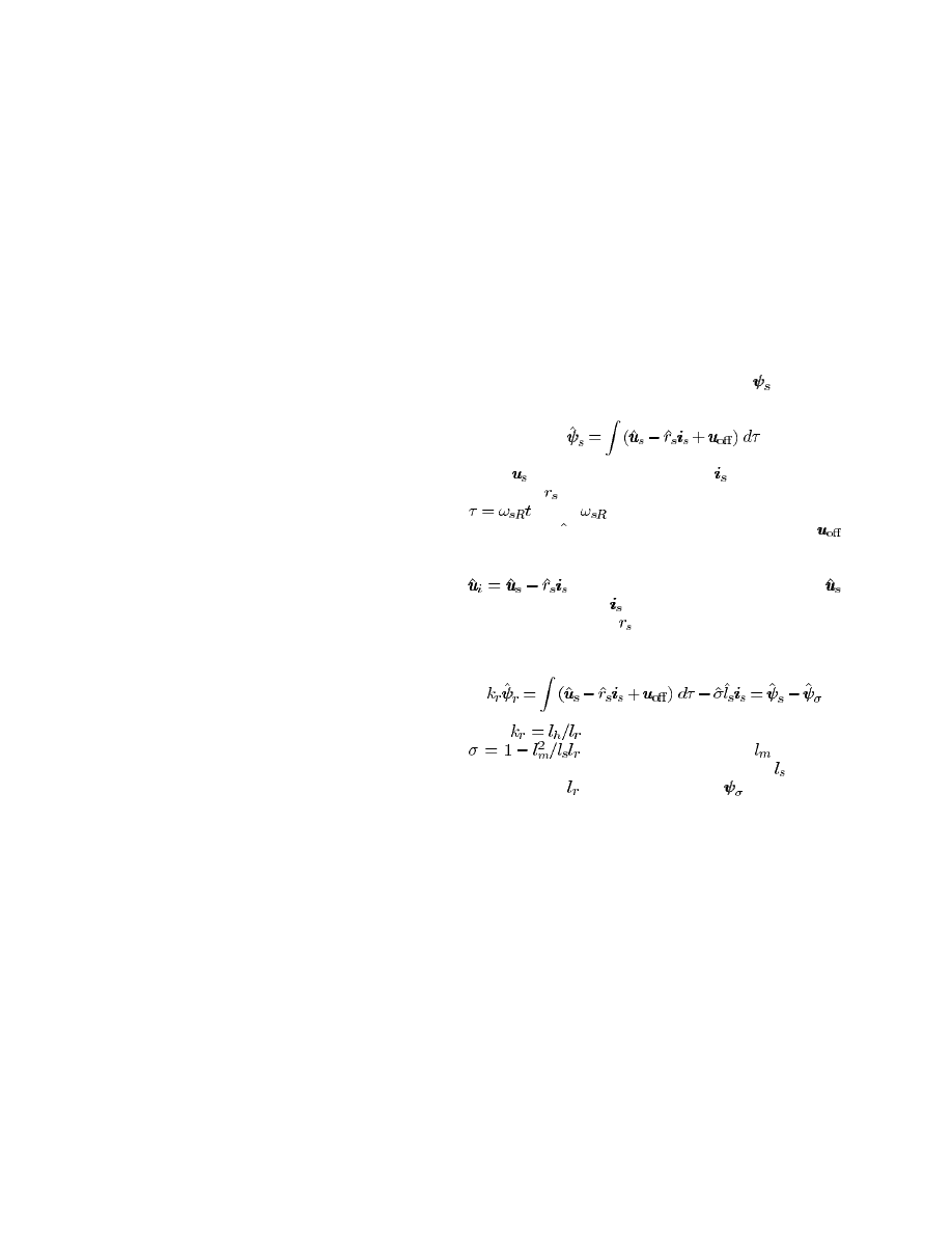
A. Estimation of the Flux Linkage Vector

Most sensorless control schemes rely directly or indirectly on

the estimation of the stator flux linkage vector

[1], [2], being

defined as the time integral of the induced voltage

(1)

where

is the stator voltage vector,

is the stator current

vector, and

is the stator resistance. Time is normalized as

, where

is the nominal stator frequency [3]. The

added symbol

marks estimated variables. The vector

in

(1) represents all disturbances such as offsets, unbalances, and
other errors that are contained in the estimated induced voltage

, resulting from either the voltage signal

or

from the current signal

. A major source of error is a mismatch

of the model parameter

.

Rotor-flux-oriented schemes estimate the rotor flux linkage

vector as

(2)

where

is the coupling factor of the rotor windings,
is the total leakage factor,

is the mutual

inductance between the stator and rotor windings,

is the stator

inductance, and

is the rotor inductance.

is the total leakage

flux vector.

The estimation of one of the flux vectors according to (1) or

(2) requires performing an integration in real time. The use of a
pure integrator has not been reported in the literature. The reason
is that an integrator has an infinite gain at zero frequency. The
unavoidable offsets contained in the integrator input then make
its output gradually drift away beyond limits. Therefore, instead
of an integrator, a low-pass filter usually serves as a substitute. A
low-pass filter has a finite dc gain which eases the drift problem,
although drift is not fully avoided. However, a low-pass filter in-
troduces severe phase angle and amplitude errors at frequencies
around its corner frequency, and even higher errors at lower fre-
quencies. Its corner frequency is normally set to 0.5–2 Hz, de-
pending on the existing amount of offset. The drive performance
degrades below stator frequencies 2–3 times this value; the drive
becomes instable at speed values that correspond to the corner
frequency.

Different ways of compensating the amplitude and phase-

angle errors at low frequencies have been proposed [4]–[7].

0093-9994/02$17.00 © 2002 IEEE

1088

IEEE TRANSACTIONS ON INDUSTRY APPLICATIONS, VOL. 38, NO. 4, JULY/AUGUST 2002

Ohtani [4] reconstructs the phase-angle and amplitude error pro-
duced by the low-pass filter. A load-dependent flux vector refer-
ence is synthesized for this purpose. This signal is transformed
to stator coordinates and then passed through a second low-pass
filter having the same time constant. The resulting error vector
is added to the erroneous flux estimate. Although the benefits
of this method are not explicitly documented in [4], improved
performance should be expected in an operating range around
the corner frequency of the low-pass filter.

With a view to improving the low-speed performance of flux

estimation, Shin et al. [5] adjust the corner frequency of the
low-pass filter in proportion to the stator frequency, while com-
pensating the phase and gain errors by their respective steady-
state values. It was not demonstrated, though, that dynamic op-
eration at very low frequency is improved. Hu and Wu [6] try to
force the stator flux vector onto a circular trajectory by propor-
tional plus integral (PI) control. While this can provide a correct
result in the steady state, it is erroneous at transient operation
and also exhibits a large error at startup. A practical application
of this method has not been reported; our investigations show
loss of field orientation following transients.

B. Acquisition of the Stator Voltages

The induced voltage, which is the signal to be integrated for

flux vector estimation, is obtained as the difference between
the stator voltage and the resistive voltage drop across the ma-
chine windings. When a voltage-source inverter (VSI) is used
to feed the machine, the stator voltages are formed by pulse
trains having a typical rise time of 2–10 kV/ s. These are dig-
itally acquired at a high, though limited sampling rate [7]. The
limited bandwidth of such sampling process may fail to estab-
lish the exact volt-second equivalent between the actual and
the acquired signals and, hence, produce an error. To avoid this
complication, some authors have used a current-source inverter
(CSI) [6], or a linear power amplifier [8], to make use of smooth
voltage waveforms that can be accurately acquired even at lim-
ited sampling rate.

To avoid this problem in a switched VSI drive, it is preferred

to replace the actual stator voltages by the reference voltage
vector that controls the pulsewidth modulator

, where

is the fundamental component of

. This very simple

method yields good results, except when operating in the
low-speed region. The respective magnitudes

and

are

then very small and the errors may even exceed the actual
signals in magnitude. One of the predominant sources of error
at very low speed is the nonlinear relationship between

and

caused by the switching characteristics of the inverter.

C. Acquisition of the Stator Currents

The stator currents are usually measured by two Hall sensors.

They are acquired as analog signals, which are subsequently
digitized using A/D converters. The sources of errors in this
process are dc offsets and gain unbalances in the analog signal
channels [9]. After the transformation of the current signals to
synchronous coordinates, dc offsets generate ac ripple compo-
nents of fundamental frequency, while gain unbalances produce
elliptic current trajectories instead of circular trajectories. The
disturbance in the latter case is a signal of twice the fundamental
frequency.

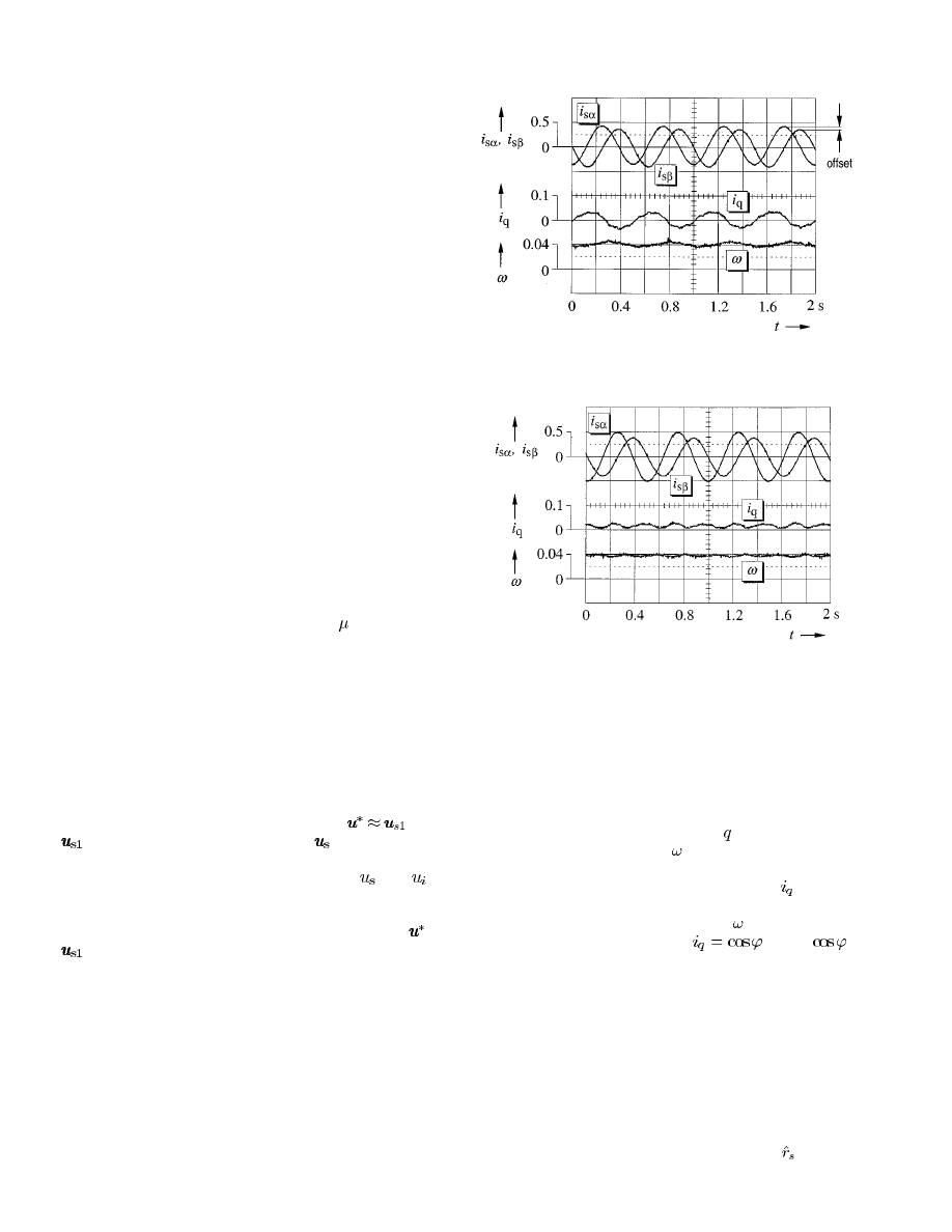
Fig. 1.

Effect of a dc offset in one of the current signals on the performance

of a vector-controlled drive system.

Fig. 2.

Effect of a gain unbalance between the acquired current signals on the

performance of a vector-controlled drive.

The following oscillograms demonstrate the effect of such

disturbances on the performance of a vector-controlled drive
system. The respective disturbances are intentionally intro-
duced, for better visibility at a higher signal level than would
normally be expected in a practical implementation.

Fig. 1 shows the effect of 5% dc offset in one of the current

signals on the no-load waveform of the -axis current, and on
the mechanical angular velocity

. The drive is operated is at a

stator frequency of 2 Hz. The transformed current signals gen-
erate oscillations in the torque-producing current

. Resulting

from this are torque pulsations of 0.06 nominal value, and cor-
responding oscillations in the speed signal . Note that nominal
torque at rated flux is produced by

, where

is

the power factor of the motor.

Fig. 2 shows the same signals under the influence of 5% gain

unbalance between the two current channels. Oscillations of
twice the stator frequency are generated in the torque-producing
current, and also in the speed signal.

D. Estimation of the Stator Resistance

Another severe issue, in addition to the integration problem

and to the nonlinear behavior of the inverter, is the mismatch be-
tween the machine parameters and the respective model param-
eters. In particular, adjusting the stator resistance

in (1) and

(2) to match its actual value is most important for accurate stator

HOLTZ AND QUAN: SENSORLESS VECTOR CONTROL OF INDUCTION MOTORS

1089

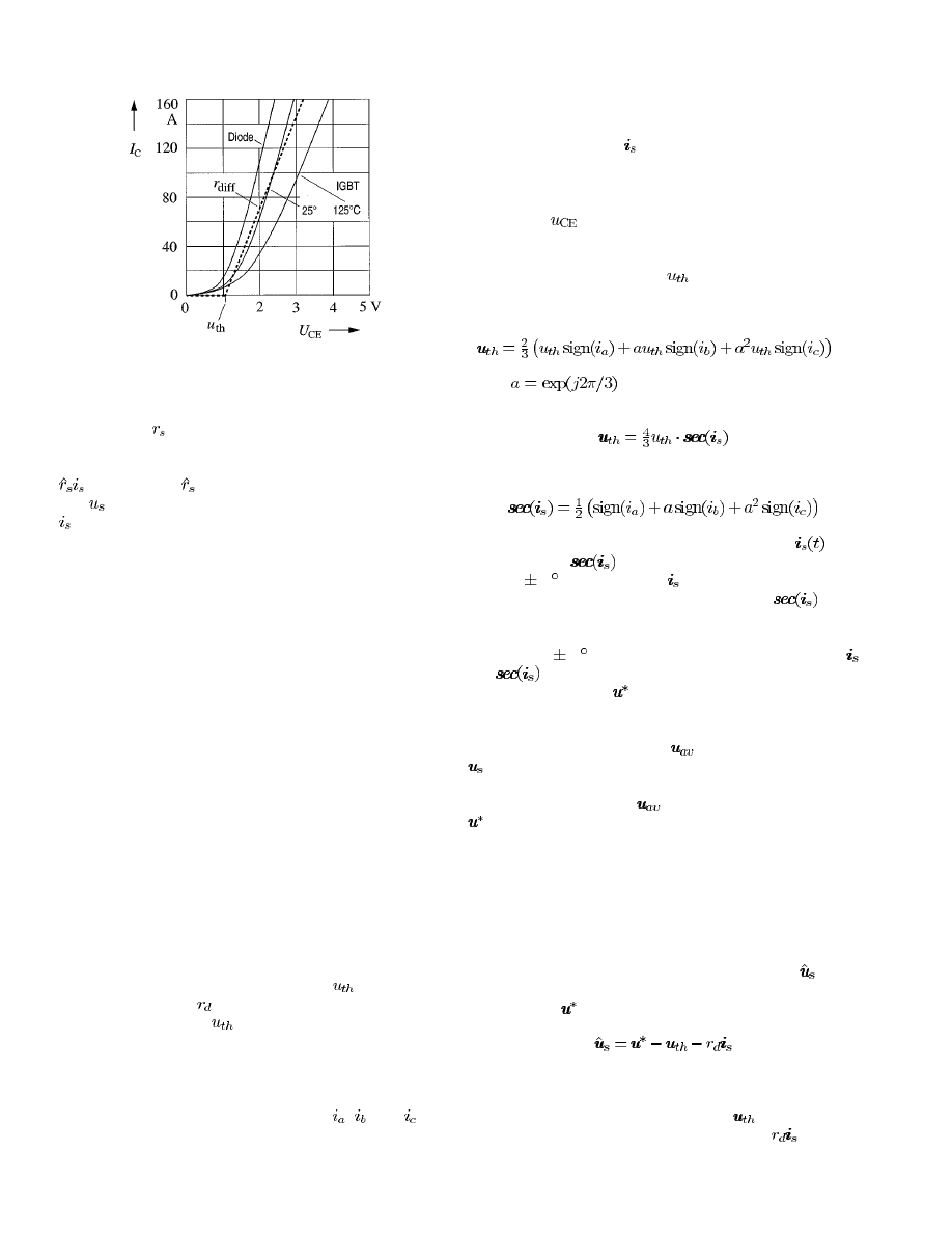
Fig. 3.

Forward characteristics of the power devices.

flux estimation, and for stable operation at very low speed. The
actual value of

varies typically in a range of about 1 : 2 due to

variations of the winding temperature. It is, therefore, apparent
from (1) and (2) that the influence of the resistive voltage drop

and, hence, of

, becomes predominant when the magni-

tude

is small, i.e., at low speed. The stator current magnitude

ranges typically between 0.3 at no load and unity at nominal

load.

Viewing the recent literature, the stator resistance is deter-

mined in [10] as the small difference between two large quan-
tities, namely real stator power and air-gap power and, as such,
the result is prone to error. The method presented in [11] re-
lies on the accuracy of other machine parameters which are not
necessarily constant, such as slip, leakage inductance, and rotor
resistance.

To overcome the aforementioned problems, this paper em-

ploys a pure integrator for stator flux estimation. Increased ac-
curacy is achieved by eliminating direct stator voltage measure-
ment. The available reference voltage signal is used instead, cor-
rected by a self-adjusting nonlinear inverter model. A third im-
provement is a novel method for on-line adaptation of the stator
resistance.

III. M

ODELS FOR

V

ERY

-L

OW

-S

PEED

O

PERATION

A. Inverter Model

At very low speed, the voltage drop in the pulsewidth mod-

ulation (PWM) inverter can be higher than the induced voltage
and, hence, constitutes a severe disturbance. The forward char-
acteristics of the power devices are shown in Fig. 3. They can
be modeled by an average threshold voltage

and an average

differential resistance

[12]. The variations with temperature

of the threshold voltage

are neglected in a first step. Thus,

the approximated forward characteristics of the power devices
are marked by the dotted line in Fig. 3.

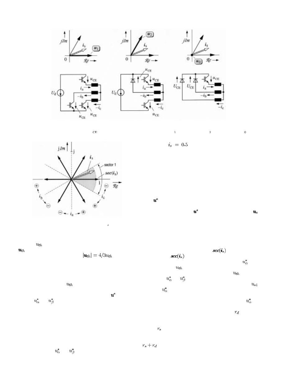
A model of the inverter is derived considering the inverter

topology during a switching sequence of one-half cycle as
shown in Fig. 4. The three phase currents

,

, and

flow

either through an active device, mostly an insulated gate
bipolar transistor (IGBT), or a recovery diode, depending on
the switching state of the inverter. The directions of the phase

currents, however, do not change in a larger time interval of
about one-sixth of a fundamental cycle. They depend only on
the stator current vector

. Fig. 4 illustrates that the effect of

the device voltage drops does not change as the switching states
change during PWM, provided that the directions of current
flow do not change. The inverter then introduces voltage
components

of about equal magnitude to all the three

phases, and it is the directions of the respective phase currents
that determine their signs.

The device threshold voltage

as defined in Fig. 3 consti-

tutes one portion of the device forward voltage. Its influence can
be described by the threshold voltage vector

(3)

where

.

Equation (3) converts into

(4)

where

(5)

is a nonlinear function of the stator current vector

. The

sector indicator

is a unity vector that indicates the re-

spective

30 sector in which

is located. Fig. 5 illustrates

the six possible locations of the sector indicator

in the

complex plane. The locations are determined by the respective
signs of the three phase currents in (3), or, in other words, by a
maximum of

30 phase displacement between the vectors

and

.

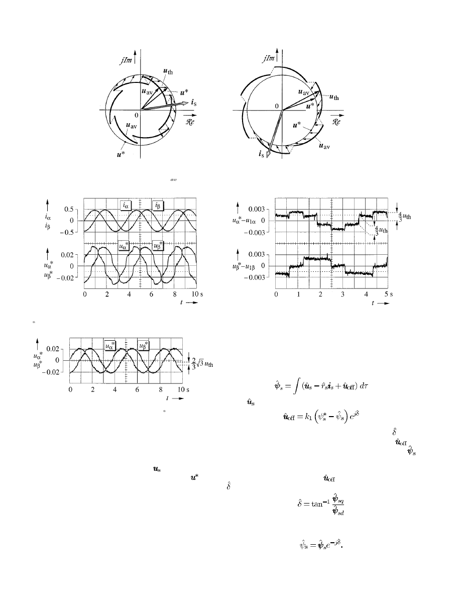
The reference signal

of the pulsewidth modulator controls

the stator voltage of the machine. It follows a circular trajec-
tory in the steady state. Owing to the forward voltages of the
power devices, the average value

of the stator voltage vector

, taken over a switching cycle, describes trajectories that re-

sult as being distorted and discontinuous. Fig. 6 shows that the
fundamental amplitude of

is less than its reference value

at motoring, and larger at regeneration. The voltage trajecto-

ries exhibit strong sixth harmonic components in addition. Since
the threshold voltage does not vary with frequency as the stator
voltage does, the distortions are more pronounced at low stator
frequency where the stator voltage is low. The distortions intro-
duced by the inverter may even exceed the commanded voltage
in magnitude, which then makes correct flux estimation and
stable operation of the drive impossible.

Using the definitions (3)–(5), an estimated value

of the

stator voltage vector can be obtained from the PWM reference
voltage vector

(6)

where the two subtracted vectors represent the total inverter
voltage vector. The inverter voltage vector reflects the respective
influence of the threshold voltages through

, and of the resis-

tive voltage drops of the power devices through

. A signal

flow graph of the inverter model (6) is shown in the left-hand
side of Fig. 10.

1090

IEEE TRANSACTIONS ON INDUSTRY APPLICATIONS, VOL. 38, NO. 4, JULY/AUGUST 2002

(a)

(b)

(c)

Fig. 4.

Effect at PWM of the forward voltages

u

of the power semiconductors. (a) Switching state

S . (b) Switching state S . (c) Switching state S .

Fig. 5.

Six possible locations of the sector indicator

sec

sec

sec(iii ); the dotted lines

indicate the transitions at which the signs of the respective phase currents
change.

Note that

is the threshold voltage of the power devices, while

is the resulting threshold voltage vector. We have, therefore,

from (4), the unusual relationship

. The reason

is that, unlike in a balanced three-phase system, all three phase
components in (3) have the same magnitude, which is unity.

B. Identification of the Inverter Model Parameters

The threshold voltage

is one parameter of the inverter

model. It is determined during a self-commissioning process
from the distortions of the reference voltage vector

. The com-

ponents

and

of the reference voltage vector are acquired

while using the current controllers to inject sinusoidal currents
of very low frequency into the stator windings. In such condi-
tion, the machine impedance is dominated by the stator resis-
tance. The stator voltages are then proportional to the stator cur-
rents. Any deviation from a sinewave of the reference voltages
that control the pulsewidth modulator are, therefore, caused by
the inverter.

As an example, an oscillogram of the distorted reference

voltage waveforms

and

, measured at sinusoidal currents

of magnitude

, is shown in Fig. 7. The amplitude

of the fundamental voltage is very low which is owed to the
low frequency of operation. The distortions of the voltage
waveforms in Fig. 7 are, therefore, fairly high. They are
predominantly caused by the dead-time effect of the inverter.
Using such distorted voltages to represent the stator voltage
signal in a stator flux estimator would lead to stability problems
at low speed. Accurate inverter dead-time compensation [13]
is, therefore, mandatory for high-performance applications.

Fig. 8 shows the same components of the reference voltage

vector

with a dead-time compensator implemented. The dis-

tortions are now much smaller, but complete linearity between
the reference voltage vector

and the stator voltage vector

is not yet achieved. The remaining periodic step changes in the
voltage waveforms are caused by the threshold voltages of the
power devices, as described by (4) and illustrated in Fig. 6.

In Fig. 6, the step changes that characterize the distorted

voltage trajectory have different magnitudes, as have the
projections of the step changes on the respective axes. These
are proportional to the sector indicator

according to (4);

the locations of

are shown in Fig. 4. It follows from (4)

that both the larger step change and the amplitude of

have

the magnitude 4/3

as indicated in Fig. 9.

Extracting the value of the threshold voltage

from the

waveform of

(or

) in Fig. 8 appears quite inaccurate. A

better method is subtracting the fundamental component
from, e.g.,

, which then yields a square-wave-like, stepped

waveform as shown in Fig. 9. The fundamental component is
easily extracted from a set of synchronous samples of

by

fast Fourier transform.

The differential resistance of the power devices,

in (6), es-

tablishes a linear relation between the load current and its in-
fluence on the inverter voltage. Functionally, it adds to the re-
sistance

of the stator windings and, hence, influences also

the transient stator time constant of the induction motor, and
on the design parameters of the current controllers. The value
(

) is estimated by an online tuning process described in

Section III-D.

HOLTZ AND QUAN: SENSORLESS VECTOR CONTROL OF INDUCTION MOTORS

1091

(a)

(b)

Fig. 6.

Effect of inverter nonlinearity. The trajectory

uu

u

represents the average stator voltage (switching harmonics excluded). (a) At motoring. (b) At

regeneration.

Fig. 7.

Effect of inverter dead time on the components of the voltage vector

uu

u , operation with injected sinewave currents; stator frequency 0.25 Hz.

Fig. 8.

Components of the reference voltage vector

uu

u as in Fig. 7; inverter

operated with dead-time compensation.

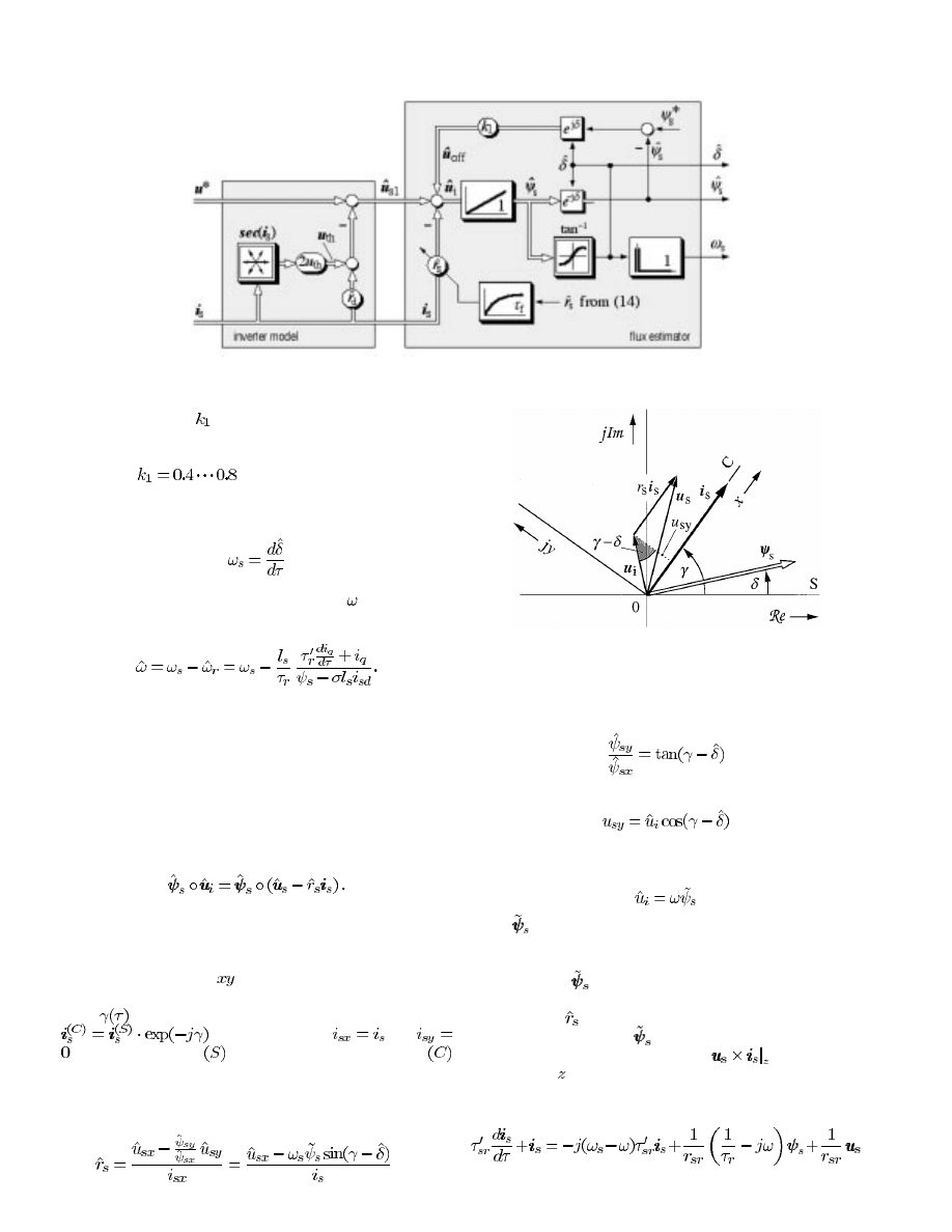
C. Stator Flux Estimation

The inverter model (6) is used to compensate the nonlinear

distortions introduced by the power devices of the inverter. The
model estimates the stator voltage vector

that prevails at the

machine terminals, using the reference voltage vector

of the

pulsewidth modulator as the input variable. The inverter model
thus enables a more accurate estimation of the stator flux linkage
vector. The signal flow graph of the inverter model is shown in
the left-hand side of Fig. 10.

The right-hand side of Fig. 10 shows the signal flow graph

of the stator flux estimator. It is a particular attraction of this
approach that the stator flux vector is obtained by pure integra-
tion. The method necessarily incorporates the estimation of a
time-varying vector that must represent the offset voltages. Im-
plementing a pure integrator avoids the usual estimation errors

Fig. 9.

Distortion voltage generated by the inverter; components in stationary

coordinates.

and bandwidth limitation associated with using a low-pass filter.
This is a particular advantage when operating at very low fre-
quency.

The defining equation of the stator flux estimator is

(7)

where

is the estimated stator voltage vector, and

(8)

is the estimated effective offset voltage vector, while

is the

estimated stator field angle. The offset voltage vector

in

(7) is determined such that the estimated stator flux vector
rotates close to a circular trajectory in the steady state, which
follows from (7) and from the right-hand side of (8).

To enable the identification of

in (8), the stator field angle

is estimated as

(9)

as illustrated in the right portion of Fig. 10. The magnitude of
the stator flux linkage vector is then obtained as

(10)

This value is used in (8) to determine the vector of the effective
offset voltage.

1092

IEEE TRANSACTIONS ON INDUSTRY APPLICATIONS, VOL. 38, NO. 4, JULY/AUGUST 2002

Fig. 10.

Signal flow graph of the inverter model and the stator flux estimator.

The gain constant

in (8) is chosen such that the ac dis-

turbances introduced by dc offsets and unbalanced gains of the
stator current acquisition channels are well compensated. Values
in the range

serve this purpose in a satisfactory

manner.

The stator frequency signal is computed by

(11)

from which the angular mechanical velocity

is determined,

for instance, with reference to [2]

(12)

D. Stator Resistance Estimation

Utilizing the inherent good low-speed performance of the

novel flux estimator requires the accurate online adaptation of
the stator resistance, which is the relevant parameter of the ma-
chine model. The proposed algorithm relies on the orthogonal
relationship in steady state between the stator flux vector and
the induced voltage. The inner product of these two vectors is

(13)

This expression depends on the stator resistance. To reduce the
online computation time for its estimation, (13) is transformed
to a reference frame that aligns with the current vector. This
current reference frame (

frame) rotates in synchronism and

is displaced with respect to stationary coordinates by the phase
angle

of the stator current, as shown in Fig. 11. We have

and, consequently,

and

. Of the superscripts,

refers to stator coordinates and

refers to current coordinates.

The estimated value of the stator resistance is obtained as the

solution of (13) in current coordinates

(14)

Fig. 11.

Vector diagram illustrating the estimation of the stator resistance;

S

marks stationary reference frame (

; ) and C marks the current reference

frame (

x; y).

using the relationships

(15)

and

(16)

which can be taken from the vector diagram Fig. 10. Further-
more, we have in a steady state

(17)

where

is an estimated stator flux value defined by (20).

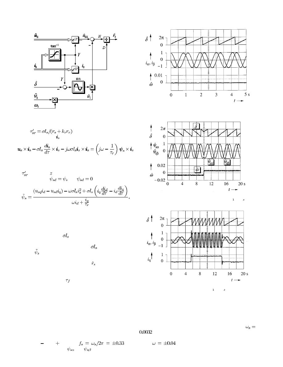
The signal flow diagram of the stator resistance adaptation

scheme is shown in Fig. 12.

The value of

in (17) cannot be obtained from the stator

flux estimator of Fig. 10 [(7)], as it would be erroneous if the
modeled value

of the stator resistance is wrongly identified.

Another estimated value,

, is therefore used, being derived

from the instantaneous reactive power

. This notation

describes the

component of the vector product of the stator

voltage and current vectors.

The system equation, for example given in [3], is

(18)

HOLTZ AND QUAN: SENSORLESS VECTOR CONTROL OF INDUCTION MOTORS

1093

Fig. 12.

Signal flow graph of the stator resistance estimator.

where

. Equation (18) is externally mul-

tiplied by the vector

, from which

(19)

is obtained. This operation eliminates the stator and the rotor re-
sistances from (18) where these parameters are there contained
in

. Taking the component of all terms in (19) and assuming

field orientation,

and

, we have

(20)

The stator flux value thus obtained does not depend on the stator
resistance. It is used in the stator resistance estimator of Fig. 12
to compute the magnitude of the induced voltage.

The stator flux vector as estimated by (20) depends on the

total leakage inductance

as the only uncertain parameter. Its

contribution to (20) represents the total leakage flux linkages
and their changes with time. An error in

has only a marginal

effect on

since the total leakage flux makes up for about only

10% of the stator flux at nominal load.

The estimated stator resistance value

from (14) is used as

an input signal to the stator flux estimator of Fig. 10. It adjusts
its parameter through a low-pass filter. The nonnormalized value
of the filter time constant

is about 100 ms.

IV. E

XPERIMENTAL

R

ESULTS

The system was implemented in a 11-kW PWM inverter-fed

induction motor drive. The machine data are: 380 V, 22 A, and
1460 r/min. A controlled dc machine was used as the load.

The oscillogram of Fig. 13 shows zero-speed operation in the

steady state at 0.9-Hz stator frequency and nominal load. The
stator currents are exactly sinusoidal and the commanded speed
is maintained without excursions. Dynamic operation at very
low speed is demonstrated by Fig. 14, showing a reversal of
speed from

10 to

10 r/min (

Hz).

The recorded components

and

of the estimated stator

Fig. 13.

Zero-speed operation at steady state and nominal load; 0.9 Hz stator

frequency.

Fig. 14.

Speed reversal at 10 r/min; fundamental frequency

f = ! =2 =

60:33 Hz.

Fig. 15.

Constant-speed operation at 5 r/min (

f = w =2p = 60:16 Hz),

with load step changes of rated magnitude applied.

flux linkage vector exhibit sinusoidal waveforms without offset,
drift, or distortion, and smooth speed operation is achieved.
Fig. 15 shows the response to load step changes of rated mag-
nitude while the speed is maintained constant at 5 r/min. This
corresponds to operating at a stator frequency of 0.16 Hz (

) during the no-load portions. Fig. 16 shows the low-

speed performance in a speed reversal process between the set
values

. The torque is held constant at a constant

value such that the drive operates in the generating mode while

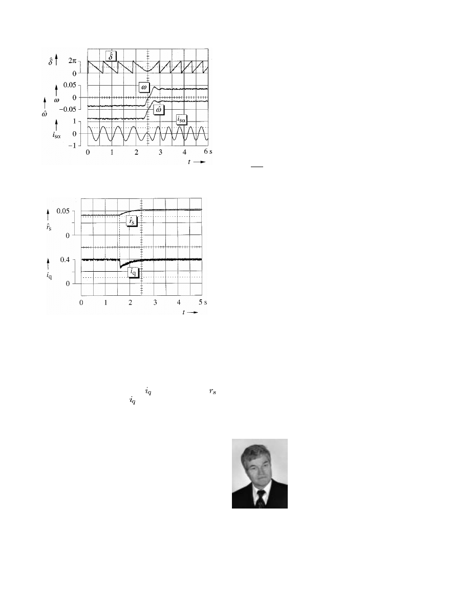
1094

IEEE TRANSACTIONS ON INDUSTRY APPLICATIONS, VOL. 38, NO. 4, JULY/AUGUST 2002

Fig. 16.

Identification of the stator resistance, demonstrated by a 30% step

increase of the resistance value.

Fig. 17.

Reversal of speed between the set-point values

w = 60:04; torque

is constant at 50% nominal value.

the speed is negative. Finally, the performance of the stator re-
sistance identification scheme is demonstrated in Fig. 17. The
stator resistance is increased by 30% in a step-change fashion.
The disturbance causes a sudden deviation from the correct field
angle, which produces a wrong value

. The new value of

is

identified after a short delay, and

readjusts to its original level.

The speed remains unaffected.

V. S

UMMARY

Physical limits make sensorless speed control at zero stator

frequency impossible when using the fundamental field repre-
sentation of the induction motor for modeling. Speed estimation
is also a problem in the neighborhood of zero stator frequency.
Noise, offset, drift, unbalances, bandwidth limits, and model pa-
rameter mismatch dominate the acquired signals which leads to
speed oscillations and instabilities. The fundamental field model
is nevertheless very attractive, as even highly sophisticated con-
trol and identification algorithms can be economically imple-
mented in modern signal processing hardware.

Making use of this situation, more accurate models of the

system components are introduced in this paper. An inverter
model serves to compensate the nonlinear distortions introduced
by the power devices, enabling a more accurate estimation of
the stator flux linkage vector. To increase the bandwidth of flux
estimation, the stator flux linkage vector is obtained by pure in-

tegration. This implies that the time-varying disturbances are
compensated by an estimated offset voltage vector. Finally, a
stator resistance estimation scheme serves to make the machine
model more accurate.

The effectiveness of these methods is demonstrated by ex-

periments. Excellent steady-state and dynamic performance is
achieved, even at extremely low speeds down to 0.003 p.u.

R

EFERENCES

[1] K. Rajashekara, Ed., Sensorless Control of AC Motors.

New York:

IEEE Press, 1996.

[2] J. Holtz, “Sensorless control of induction motor drives,” Proc. IEEE, to

be published.

[3]

, “The representation of AC machine dynamics by complex signal

flow graphs,” IEEE Trans. Ind. Electron., vol. 42, pp. 263–271, June
1995.

[4] T. Ohtani, N. Takada, and K. Tanaka, “Vector control of induction motor

without shaft encoder,” IEEE Trans. Ind. Applicat., vol. 28, pp. 157–165,
Jan./Feb. 1992.

[5] M.-H. Shin, D.-S. Hyun, S.-B. Cho, and S.-Y. Choe, “An improved stator

flux estimation for speed sensorless stator flux orientation control of
induction motors,” IEEE Trans. Power Electron., vol. 15, pp. 312–318,
Mar. 2000.

[6] J. Hu and B. Wu, “New integration algorithms for estimating motor flux

over a wide speed range,” IEEE Trans. Power Electron., vol. 13, pp.
969–977, Sept. 1998.

[7] X. Xu and D. W. Novotny, “Implementation of direct stator flux oriented

control on a versatile DSP based system,” IEEE Trans. Ind. Applicat.,
vol. 29, pp. 694–700, Mar./Apr. 1991.

[8] K. Akatsu and A. Kawamura, “Sensorless very low-speed and zero-

speed estimations with online rotor resistance estimation of induction
motor without signal injection,” IEEE Trans. Ind. Applicat., vol. 36, pp.
764–771, May/June 2000.

[9] D.-W. Chung and S.-K. Sul, “Analysis and compensation of current mea-

surement error in vector-controlled AC motor drives,” IEEE Trans. Ind.
Applicat., vol. 34, pp. 340–345, Mar./Apr. 1998.

[10] I.-J. Ha and S.-H. Lee, “An online identification method for both

stator and rotor resistances of induction motors without rotational
transducers,” IEEE Trans. Ind. Electron., vol. 47, pp. 842–853, Aug.
2000.

[11] M. Depenbrock, “Speed sensorless control of induction motors at very

low stator frequencies,” in Proc. European Conf. Power Electronics and
Applications, 1999.

[12] J.-W. Choi and S.-K. Sul, “Inverter output voltage synthesis using novel

dead time compensation,” IEEE Trans. Power Electron., vol. 11, pp.
221–224, Mar. 1996.

[13] Y. Murai, T. Watanabe, and H. Iwasaki, “Waveform distortion and

correction circuit for PWM inverters with switching lag-times,” IEEE
Trans. Ind. Applicat., vol. IA-23, pp. 881–886, Sept./Oct. 1987.

Joachim Holtz (M’87–SM’88–F’93) graduated in
1967 and received the Ph.D. degree in 1969 from the
Technical University Braunschweig, Braunschweig,
Germany.

In 1969, he became an Associate Professor and, in

1971, he became a Full Professor and Head of the
Control Engineering Laboratory, Indian Institute of
Technology, Madras, India. In 1972, he joined the
Siemens Research Laboratories, Erlangen, Germany.
From 1976 to 1998, he was a Professor and Head of
the Electrical Machines and Drives Laboratory, Wup-

pertal University, Wuppertal, Germany. He is currently a Consultant. He has
authored more than 120 technical papers, including 70 refereed publications in
journals. He has also authored 17 invited conference papers and ten invited pa-
pers published in journals. He is the coauthor of four books and the holder of
29 patents.

Dr. Holtz was the recipient of the IEEE Industrial Electronics Society Dr. Eu-

gene Mittelmann Achievement Award, the IEEE Industry Applications Society
Outstanding Achievement Award, the IEEE Power Electronics Society William
E. Newell Field Award, the IEEE Third Millenium Medal, and the IEEE Lamme
Gold Medal. He has earned six IEEE Prize Paper Awards.

HOLTZ AND QUAN: SENSORLESS VECTOR CONTROL OF INDUCTION MOTORS

1095

Juntao Quan was born in Jiangxi, China, in 1964. He
received the B.Eng. degree from Jiangxi Polytechnic
College, Nanchang University, Nanchang, China,
the M.Eng. degree from Northeast-Heavy Mechanic
Institute, Yanshan University, Qinhuangdao, China,
and the Ph.D. degree from Wuppertal University,
Wuppertal, Germany, in 1983, 1989, and 2002,
respectively, all in electrical engineering.

He was an Assistant Electrical Engineer for three

years at the Nanchang Bus Factory, Nanchang, China.
From 1989 to 1994, he was a Lecturer at Yanshan

University. During this time, he also worked on various projects for applications
of power electronics. In 1995, he joined the Electrical Machines and Drives Lab-
oratory, Wuppertal University, where he worked and studied toward the Ph.D.
degree. In June 2000, he joined the Danaher Motion Group, Kollmorgen-Seidel,
Duesseldorf, Germany. His main interests are in the areas of adjustable-speed
drives, microprocessor-embedded real-time control, power electronics applica-
tions, and advanced motion control.