Lecture 6: Goodness of Fit tests

Probability and

Statistics
Part 2: Statistics

Goodness of Fit tests



These statistical methods test
nominal scale data to determine if
the observed distribution of

counts

(never percentages or ratios) fits a
hypothesized distribution.



The most notable analysis
technique is the chi-square (χ

2

)

test.

Introduction



Assume that a geneticist has
carried out a crossing experiment
between two F

1

hybrids and

obtains an F

2

progeny of 90

offspring, n

1

=80 of which appear

to be wild-type and n

2

=10 of which

are the mutant phenotype.

Introduction



The geneticist assumed dominance
and expected a ratio of 3:1 of the
phenotypes, but the actual ratio is
80/10 = 8:1.



Expected values of p and q are

for wild-type and mutant respectively.

25

.

0

q

ˆ

75

.

0

p

ˆ





and

Introduction



We use ‘hat’ to indicate hypothetical
or expected values of binomial
proportions.



The observed proportions of these
two classes are

respectively.

11

.

0

q

89

.

0

p

90

10

90

80









and

Introduction



Another way of noting the contrast
between observation and
expectation is to state it in counts
(some authors say frequencies).

Introduction



The observed counts are n

1

=80 and

n

2

=10 for the two phenotypes.



The expected counts are

where N refers to the sample size of
offspring from the cross.

5

.

22

N

25

.

0

N

q

ˆ

n

ˆ

5

.

67

90

75

.

0

N

p

ˆ

n

ˆ

2

1





















Introduction



The obvious question is whether
the deviation from 3:1 hypothesis
observed in our sample is of such a
magnitude as to be improbable.



In other words, do the observed
data differ enough from expected
values to cause to reject the null
hypothesis?

Exact distribution
approach



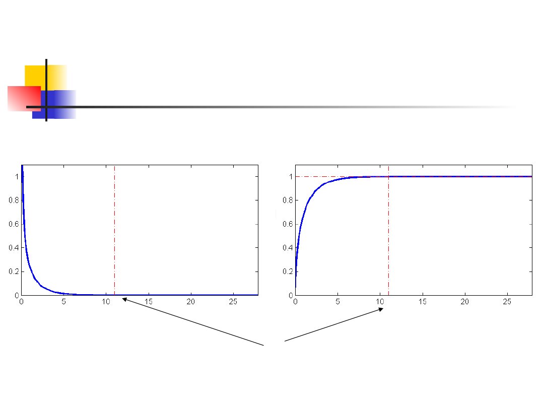
This is a binomial distribution in which p
is the probability of being a wild-type and
q is the probability of being a mutant.



We can work out the probability of
obtaining an outcome of 80 wild-type
phenotypes and 10 mutants, as well as
all ‘worse’ cases in sample of 90 offspring
for

25

.

0

q

ˆ

75

.

0

p

ˆ





and

Exact distribution
approach

which is equal to the cumulative
probability of the tail of the
distribution.





























90

80

k

k

N

k

90

80

k

k

N

k

q

ˆ

p

ˆ

)!

k

N

(

!

k

!

N

q

ˆ

p

ˆ

k

N

Exact distribution
approach



The result is a probability of
0.00084895 for all outcomes as
deviant or more deviant from the
hypothesis.



Note this is a one-tailed test, the
alternative hypothesis being that there
are more wild-type offspring than the
Mendelian hypothesis would postulate.

Exact distribution
approach



The observed sample is a very
unusual outcome, and we conclude
that there is a significant deviation
from expectation.

Confidence limit approach



A less-time consuming approach
based on the same principle is to
look up confidence limits for the
binomial proportions.

Goodness of fit test (GoF
test)



We will develop a third approach to
evaluating the null hypothesis –
done by goodness of fit test.



The table will illustrate how we
might proceed.

Log-likelihood ratio test

Phenoty

pes

Observe

d counts

Observe

d

proportio

ns

Expected

proportio

ns

Expected

counts

Counts

ratio

observed

over

expected

Wild-

type

80

0.89

0.75

67.5

1.185185 13.59192

Mutant

10

0.11

0.25

22.5

0.444444 -8.10930

Sum

90

1.0

1.0

90.0

Ln L =

5.48262













i

i

i

n

ˆ

n

ln

n

Log-likelihood ratio test



The log-likelihood ratio test for
goodness of fit may be developed as
follows:
The probability of observing the
sample result assuming the population
parameter equals to sample proportion
is the same as

1326838

.

0

90

10

90

80

90

80

10

80







































Log-likelihood ratio test

The probability of observing the
sample result assuming proportions
given by Mendelian null hypothesis is
equal to

0005518

.

0

4

1

4

3

90

80

10

80







































Log-likelihood ratio test

If the observed proportions is equal to
proportion postulated under the null
hypothesis, then the two computed
probabilities will be equal, and their ratio, L,
will equal 1.
The greater the difference between
proportions the higher deviation of L from 1.

Log-likelihood ratio test

The ratio of these two probabilities or
likelihoods can be used as a statistics to
measure the degree of agreement
between sampled and expected counts.

A test based on such ratio is called a

likelihood ratio test

.

Log-likelihood ratio test

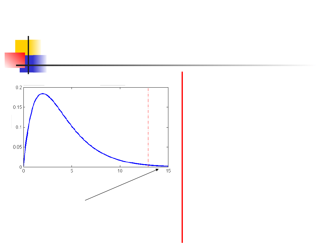
It has been shown that the distribution
of

G = 2 ln L

can be approximated by the χ

2

distribution with 1 degree of freedom.

Log-likelihood ratio test

In our case

G = 2 ln L = 10.96524

If we compare this observed value with a

χ

2

distribution with 1 degree of

freedom, we find that result is
significant

(p-value = 0.000928 < 0.001)

Chi-squared distribution,
1df

10.96524

Computational formula

2

1

2

1

2

1

n

n

n

n

1

n

n

1

q

ˆ

q

p

ˆ

p

q

ˆ

p

ˆ

n

n

q

p

n

n

L





















































Since

q

ˆ

n

n

ˆ

nq

n

p

ˆ

n

n

ˆ

np

n

2

2

1

1









2

1

n

2

2

n

1

1

n

ˆ

n

n

ˆ

n

L



























then





























2

2

2

1

1

1

n

ˆ

n

ln

n

n

ˆ

n

ln

n

L

ln

and

G test for GoF for more than
two classes



The test for goodness of fit can be applied to
a distribution with more than two classes.



Again we calculate ratios of observed over
expected counts.



The sum yields to ln L, while G = 2 ln L
follows approximately the chi-squared
distribution with a-1 degrees of freedom,
where a stands for the number of classes.

Example 1



Testing the choice of salmon
to select a certain home
stream versus four nearby
streams.

N = 200

fish

Home

stream

Stream

1

Stream

2

Stream

3

Stream

4

Observe

d

counts

135

15

17

10

23

Example 1

Hypotheses:

H

0

: Home stream is chosen 75% of

the time; remaining four streams
25% of the time (6.25% each).

H

a

: not H

o

Example 1



The null hypothesis can be
alternatively stated as
H

0

: the sample came from a

salmon population with a
12:1:1:1:1 ratio of choosing home
and alternate steams.
H

a

: not H

0

.

Example 1

Observed
counts

Expected
counts

Ratio

Home
stream

135

150

0.90

-14.2237

Stream 1

15

12.5

1.20

2.7348

Stream 2

17

12.5

1.36

5.2272

Stream 3

10

12.5

0.80

-2.2314

Stream 4

23

12.5

1.84

14.0246

Sum

200

200

ln L =
5.5315

i

n

ˆ

i

n

i

i

n

ˆ

/

n













i

i

n

ˆ

n

i

ln

n

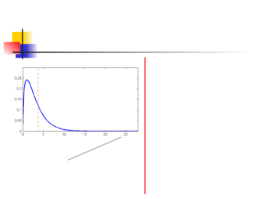
Example 1

0259

.

0

}

063

.

11

{

P

:

value

p

2

]

4

[









0.05

at

H

reject

we

G

G

since

4877

.

9

063

.

11

L

ln

2

G

0

2

]

4

[

05

.

0

crit

2

]

4

[

05

.

0



















Chi-squared test for GoF



This is an alternative technique,
the traditional approach that is
applied in substantial number of
research publications.



We turn once more to the genetic
cross with 80 wild-type and 10
mutant individuals.

Chi-squared test for GoF



First we calculate the deviations of
observed from expected counts and
square them.



In the next step we make each
deviation relative to the expected
counts.



Finally we find sum of these
quantities.

Chi-squared test for GoF



The obtained statistic is so-called
chi-squared statistic X

2

, but is only

approximately distributed as chi-
square with 1 degree of freedom

.



Some authors have called X

2

the

Pearson statistic.



The chi-squared test is always one-
tailed!!

Chi-squared test for GoF

Phenoty

pes

Observe

d counts

Expected

proportio

ns

Expected

counts

Squared

deviation

s

Relative

squared

deviation

s

Wild-

type

80

0.75

67.5

156.25

2.3148

Mutant

10

0.25

22.5

156.25

6.9444

Sum

90

1.0

90.0

X

2

=

9.2592

Chi-squared test for GoF

0023

.

0

}

2592

.

9

{

P

:

value

p

1

]

1

[









0.05

at

H

reject

we

X

since

8415

.

3

2592

.

9

X

0

2

]

1

[

05

.

0

2

2

]

1

[

05

.

0

2















Chi-squared test for GoF for
more than two classes



The chi-squared test for goodness of fit
can be applied to a distribution with more
than two classes.



Calculate:



X

2

statistic follows approximately the chi-

squared distribution with a-1 degrees of
freedom, where a stands for the number
of classes.











a

i

2

i

i

2

n

ˆ

n

ˆ

n

X

Example 1 – cont.

Observed
counts

Expected
counts

Deviation Relative

deviation
s

Home
stream

135

150

225

1.50

Stream 1

15

12.5

6.25

0.50

Stream 2

17

12.5

20.25

1.62

Stream 3

10

12.5

6.25

0.50

Stream 4

23

12.5

110.25

8.82

Sum

200

200

X

2

=12.94

i

n

ˆ

i

n





2

i

i

n

ˆ

n 

Example 1 – cont.

0116

.

0

}

94

.

12

{

P

:

value

p

2

]

4

[









0.05

at

H

reject

we

X

since

4877

.

9

94

.

12

X

0

2

]

4

[

05

.

0

2

2

]

4

[

05

.

0

2















Subdividing the chi-square
analysis



In our salmon example, the number
of fish returning to Stream 4 seems
to have caused the H

0

rejection.



So we will subdivide it.



Now let’s test H

0

: The sample came

from a salmon population with
12:1:1:1 ratio of choosing home and
alternate streams 1-3.

Example 1 – subdivision

Observed
counts

Expected
counts

Deviation Relative

deviation
s

Home
stream

135

177*12/1

5=141.6

43.56

0.3076

Stream 1

15

177*1/15

=11.8

10.24

0.8678

Stream 2

17

11.8

27.04

2.2915

Stream 3

10

11.8

3.24

0.2746

Sum

177

X

2

=3.741

5

i

n

ˆ

i

n





2

i

i

n

ˆ

n 

Example 1 – subdivision

2908

.

0

}

7415

.

3

{

P

:

value

p

2

]

3

[









0.05

at

H

reject

not

do

we

X

since

8174

.

7

7415

.

3

X

0

2

]

3

[

05

.

0

2

2

]

3

[

05

.

0

2















Continuity corrections



G or X

2

statistic values calculated

based on actual data belong to a
discrete distributions.



However, the theoretical chi-square
distribution is continuous.



With an uncorrected values you
falsely reject H

0

to often (type I error

is higher than intended one).

Continuity corrections



This is a serious problem in case of

2 classes. If N<200 we must apply

the continuity corrections.



G test – Williams’s correction



X

2

test – Yates correction

q

G

G

,

N

2

1

1

q

adj



















2

i

2

i

i

2

adj

n

ˆ

5

.

0

n

ˆ

n

X

Testing again other
distributions



We can apply GoF test to verify the
hypothesis on our data following
other than binomial distributions.



If we estimate the parameters of
the distribution (even the binomial
one) with the use of our data,
we must correctly set the number of
degrees of freedom.

Testing again other
distributions

Distribution

Parameters

estimated

from

sample

Degrees of

freedom

Binomial

p

a-2

Normal

μ,σ

a-3

Poisson

μ

a-2

Kolmogorov-Smirnov test



A nonparametric test that is applicable
to continuous frequency distributions,
where it has greater power than the G-
or chi-square tests for GoF, is the
Kolmogorov-Smirnov (KS) test.



KS test for GoF is especially useful
with small samples, it is inadvisable to
group classes.

Kolmogorov-Smirnov test



This test is based on differences
between two cumulative relative
frequency distributions, between the
observed and expected distribution.



It should be also used for discrete data
in ordered categories.



It is better than standard chi-square test,
because it takes into account the
ordering of the categories.

Kolmogorov-Smirnov test



The test for discrete data looks at the
cumulative observed and expected
counts and takes

the largest

difference

:

This value is compared to a critical
value, where k=number of categories,
N=sample size, α = alpha-level

i

i

i

max

Fˆ

F

max

d

max

d







N

,

k

,

max,

crit

d

d





Example 2 – discrete data



We want to test if insect species
are uniformly distributed along a
light gradient.



Light gradients do not have a
measurable differences, except
that lower values represent darker
light conditions than higher
numbers.

Example 2



H

0

: Insect species uniformly

distributed along a light gradient



H

a

: not H

0



We set α = 0.05

Example 2

N=65

Dark - 1

2

3

4

Light - 5

Observe

d counts

0

7

6

38

14

Expecte

d counts

13

13

13

13

13

Observe

d

cumulati

ve

counts

0

7

13

51

65

Expecte

d

cumulati

ve

counts

13

26

39

52

65

|d

i

|

13

19

26

1

0

Example 2



Test statistic

d

max

= 26



Critical value

d

max,0.05,5,65

= 10 (see

table)



Decision rule

: reject H

0

if d

max

≥10;

otherwise, do not reject.



Since 26>10 (p<0.001), we reject
H

0

.

Example 2



Conclusion:

The observed data do not follow an
uniform distribution across the
ordered light categories (p<0.001).

KS test for GoF – continuous
data



An important fact is that since
expected cumulative frequency
distribution is a continuous function,
the largest difference between
expected and observed is found by
computing differences both before and
after each time observed cumulative
frequency function steps up.