Advanced Methods for Development of Wind turbine models for control designe

XCEL RDF Project CWO2

Advanced Methods for

Development of Wind Turbine

Models for Control Design

Final Report

October 1, 2003

Submitted to:

Xcel Energy – Renewable Development Fund

414 Nicollet Mall – Ren Square 5

Minneapolis, MN 55401-1993

Prepared by:

Global Energy Concepts, LLC

5729 Lakeview Dr. NE, Suite 100

Kirkland, WA 98033

Ph: (425) 822-9008

Fx: (425) 822-9022

www.globalenergyconcepts.com

Timothy J. McCoy

Principal Investigator

RDF Project CW02

Final Report

Global Energy Concepts, LLC

October 1, 2003

Table of Contents

1 INTRODUCTION..................................................................................................... 1

1.1

ACKGROUND

...................................................................................................... 1

1.2

ROJECT

COPE AND

BJECTIVES

........................................................................ 1

2 APPROACH.............................................................................................................. 2

2.1

VERVIEW

........................................................................................................... 2

2.2

ADAMS

ODELING

............................................................................................ 3

2.2.1

Structural Model ......................................................................................... 3

2.2.2

Controls....................................................................................................... 5

2.2.3

Aerodynamics.............................................................................................. 6

2.2.4

Coordinate Systems..................................................................................... 7

2.3

INEARIZATION

.................................................................................................... 9

2.3.1

Background ................................................................................................. 9

2.3.2

ADAMS Linear.......................................................................................... 11

2.3.3

Aerodynamic Linearization....................................................................... 11

2.3.4

Linearization of Rotational Effects ........................................................... 13

3 VALIDATION AND RESULTS............................................................................ 22

3.1

ESPONSE

ALCULATIONS

................................................................................ 22

3.2

ODAL

NALYSIS

............................................................................................. 28

3.3

ONTROLS

......................................................................................................... 32

3.3.1

Model Reduction ....................................................................................... 32

3.3.2

State Feedback and Kalman Filtering ...................................................... 32

3.3.3

Example Results ........................................................................................ 33

4 CONCLUSIONS ..................................................................................................... 37
5 REFERENCES........................................................................................................ 38
Appendix A – Generalized Force Subroutine Code

Appendix B – ADAMS Model Elements

RDF Project CW02

Final Report

Global Energy Concepts, LLC

iii

October 1, 2003

List of Figures

Figure 1. Overview of Phase I approach............................................................................ 3

Figure 2. Schematic of the turbine model.......................................................................... 4

Figure 3. Generator torque speed curve............................................................................. 5

Figure 4. Blade pitch actuator controller block diagram ................................................... 6

Figure 5. Global (X,Y,Z) and blade (x,y,z) coordinate systems........................................ 7

Figure 6. Coleman X displacements a) symmetrical b) sine c) cosine ........................... 8

Figure 7. Coleman Y displacements a) symmetrical b) sine c) cosine ........................... 8

Figure 8. Coleman Z displacements a) symmetrical b) sine c) cosine............................ 8

Figure 9. Outline of methodology for linearization of rotational effects......................... 14

Figure 10. Response of the blade pitch to a step change in: a) symmetrical b) sine c)

cosine pitch demand while operating in steady 24 m/s winds.................................. 23

Figure 11. Response of rotor rpm and tower motion to a step change in: a) symmetrical

pitch demand b) wind speed c) generator torque while operating in steady 24 m/s

winds......................................................................................................................... 24

Figure 12. Response of the blade tip Coleman x direction deflection to a step change in:

a) symmetrical b) sine c) cosine pitch demand while operating in steady 24 m/s

winds......................................................................................................................... 25

Figure 13. Response of the blade tip Coleman y direction deflection to a step change in:

a) symmetrical b) sine c) cosine pitch demand while operating in steady 24 m/s

winds......................................................................................................................... 26

Figure 14. Response of the blade tip Coleman torsional deflection to a step change in: a)

symmetrical b) sine c) cosine pitch demand while operating in steady 24 m/s winds

................................................................................................................................... 27

Figure 15. Campbell diagram for the example 1.5 MW turbine...................................... 28

Figure 16. Wind speed Campbell diagram for the example 1.5 MW turbine.................. 30

Figure 17. System pole loci for the example 1.5 MW turbine......................................... 30

Figure 18. System pole loci for the example 1.5 MW turbine......................................... 31

Figure 19. Pole loci for the rotor and drive train rigid body rotation .............................. 31

Figure 20. State space control flow diagram ................................................................... 34

Figure 21. Plant and closed loop poles of the LTI model at 24 m/s ................................ 34

Figure 22. Turbine rpm in 24 m/s turbulence .................................................................. 35

Figure 23. Collective blade pitch in 24 m/s turbulence ................................................... 35

Figure 24. Drive train torques in 24 m/s turbulence ........................................................ 36

Figure 25. Electrical power in 24 m/s turbulence ............................................................ 36

Figure 26. Wind sped estimate versus actual hub height wind speed.............................. 37

RDF Project CW02

Final Report

Global Energy Concepts, LLC

October 1, 2003

List of Tables

Table 1. Complex Wind Turbine Model Description ........................................................ 4

Table 2. Complex Model Component Description............................................................ 4

Table 3. Blade Pitch Actuator Control Gains .................................................................... 5

Table 4. Model Aerodynamic Section Properties .............................................................. 6

Table 5. Linearized Model States .................................................................................... 10

Table 6. Linearized Model Inputs.................................................................................... 10

Table 7. Linearized Model Outputs ................................................................................. 10

Table 8. Perturbations for Aerodynamic Derivative Calculation .................................... 13

Table 9. Aerodynamic Derivatives .................................................................................. 13

Table 10. Modal Frequencies for Example 1.5 MW Turbine.......................................... 29

Table 11. Modes Included for a Reduced Order Model .................................................. 32

RDF Project CW02

Final Report

Global Energy Concepts, LLC

October 1, 2003

1 Introduction

1.1 Background

Over the past few years, wind turbine research and design has become increasingly

concerned with control system design. This concern arises for several reasons: turbines

have become larger, control system hardware has become more powerful, controls are

another way to drive down costs and increase performance, and turbine modeling tools

have become more sophisticated.

There are significant benefits to be gained from developing sophisticated control schemes

for variable-pitch and/or variable-speed wind turbines. These benefits generally fall into

two categories: improved energy capture and reduced loading. While both of these

benefits have potential to reduce the cost of wind energy, the latter has only seen limited

application in commercial wind turbines [1].

One of the reasons for this is that the design of sophisticated control systems for complex

structures requires models of equal sophistication and accuracy. These models must be

cast with physical and mathematical structures that integrate with control design methods

and software. While much progress has been made in recent years modeling wind

turbine structural and aerodynamic response in the time domain, obtaining detailed and

accurate system models for wind turbine control design has proven to be difficult for a

variety of reasons.

One of the primary difficulties is that the large, flexible blades, due to their rotation,

cause problems in the development of the linear models required for control design.

Another difficulty is incorporating the aeroelastic response of the structure into the

system model used for control design.

1.2 Project Scope and Objectives

There are several approaches that have potential to solve this problem. One approach

currently being investigated is the development of a structural model that will allow for

easy extraction of the system model required by the control system design tools [2,3].

While this approach has technical merit, the development process is long and costly, and

the end product is a complex simulation code that will need to be validated, maintained,

and extended as wind turbine design concepts change. Also, many of the capabilities of

this type of new code will duplicate other codes that are currently available to wind

turbine designers and researchers.

Two general alternative approaches exist that leverage an existing commercial general-

purpose structural dynamics code to extract a linearized system model: (1) use of a

commercially available linearization add-on, or (2) use of system identification

techniques to obtain a realization of the linearized system model. The advantage to both

of these approaches is that most of the complex software development has already been

done so that the method development will likely be less expensive and more rapid. Also,

RDF Project CW02

Final Report

Global Energy Concepts, LLC

October 1, 2003

the above methods will be inherently more flexible and able to accommodate different

turbine design concepts since the commercially available code is extremely powerful and

flexible.

Wind turbines are often modeled in the ADAMS [4,5] general purpose structural

dynamic analysis code, available from MSC Software of Santa Ana, California. This

code is commercially available, extremely flexible, and the necessary aerodynamic

modules needed for wind turbine analysis have been developed and validated by the

National Renewable Energy Laboratory [6,7]. While ADAMS is an extremely powerful

tool for the structural dynamic analysis of wind turbines, researchers and designers have

had difficulty using these models for developing controls algorithms.

The focus of this effort is to develop methods that allow for control development based

on the ADAMS models. Based on the results of Phase I, documented in the Phase I

report [8], the approach selected uses the add-on ADAMS linearization package in

conjunction with custom subroutines for inclusion of rotational and aerodynamic effects.

This approach was further developed and validated in Phase II. Additionally, the

resulting linear models have been used in example control design efforts.

2 Approach

2.1 Overview

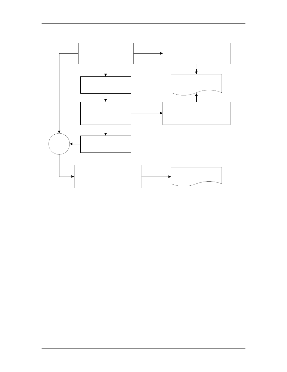
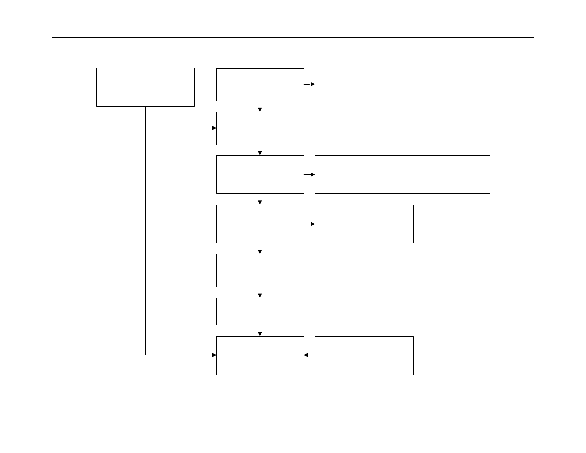
This project was broken down into two phases. In Phase I, most of the work focused on a

relatively simple model of a wind turbine where the major structural components (blades

and tower) were modeled as rigid bodies. Methods were developed and validated for the

rotational and aerodynamic effects. Figure 1 shows the basic approach used for

validation. This effort is documented in the Phase I report [8].

In Phase II, the selected techniques were applied to complex wind turbine models. In

addition to the aerodynamics, the models used discretizations of the major structural

components into multiple parts with inertial properties (mass and inertia) connected by

flexible elements. These flexible connections resemble the beam elements used in finite

element analysis. The use of complex models revealed a number of subtleties and some

flaws in the original formulation for inclusion of the rotational effects. In Phase II, a

significant effort was made to improve and validate the methodology.

RDF Project CW02

Final Report

Global Energy Concepts, LLC

October 1, 2003

Simple ADAMS Model

Running at a steady

state operating point

Linearization

Import linearized

model into Matlab

In Matlab, simulate response

to step changes in inputs

(pitch, generator torque, wind

speed)

Simulate response to step

changes in inputs (pitch,

generator torque, wind speed)

Control Design

Compare Response

(no control)

Integrate

Simulate response to step

change in disturbance input

(wind speed)

Review response of

controlled turbine

Figure 1. Overview of Phase I approach

2.2 ADAMS Modeling

2.2.1 Structural Model

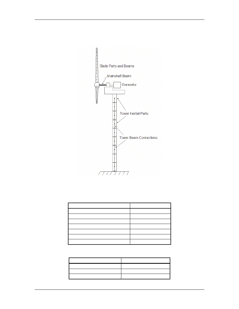
A full complex model of a wind turbine in ADAMS consists of a large number of

individual components. In particular, the blades and tower are represented by a number

of individual inertial parts connected with beam or field elements. Each individual part

has six displacement degrees of freedom, unless otherwise constrained. The main shaft is

represented by a single beam element overhung from the main bearing. The model used

primarily in the Phase II effort is shown in Figure 2 and described in

Table 1 and

Table 2.

The model used in Phase II is adapted from the work by Malcolm and Hansen [9]. It is

similar in basic architecture to the simple model the Phase I report [8]. However, the

blades have a slimmer profile, run at a higher tip speed ratio and have structural

properties that include a high degree of flap-twist coupling. Also, the tower is softer.

RDF Project CW02

Final Report

Global Energy Concepts, LLC

October 1, 2003

Figure 2. Schematic of the turbine model

Table 1. Complex Wind Turbine Model Description

Item

Value

Rating, kW

1500

Rotor diameter, m

Design tip speed ratio

7.5

Rated wind speed, m/s

11.5

Rated rpm

21.2

Hub height, m

Nacelle Tilt/Blade Coning

Table 2. Complex Model Component Description

Component

Mass, kg

Tower

434,171

Bedplate

49,801

Generator + HS shaft

1,562

RDF Project CW02

Final Report

Global Energy Concepts, LLC

October 1, 2003

LS shaft

1,562

Hub, incl pitch bearings

11,513

3 Blades, each

2,957

2.2.2 Controls

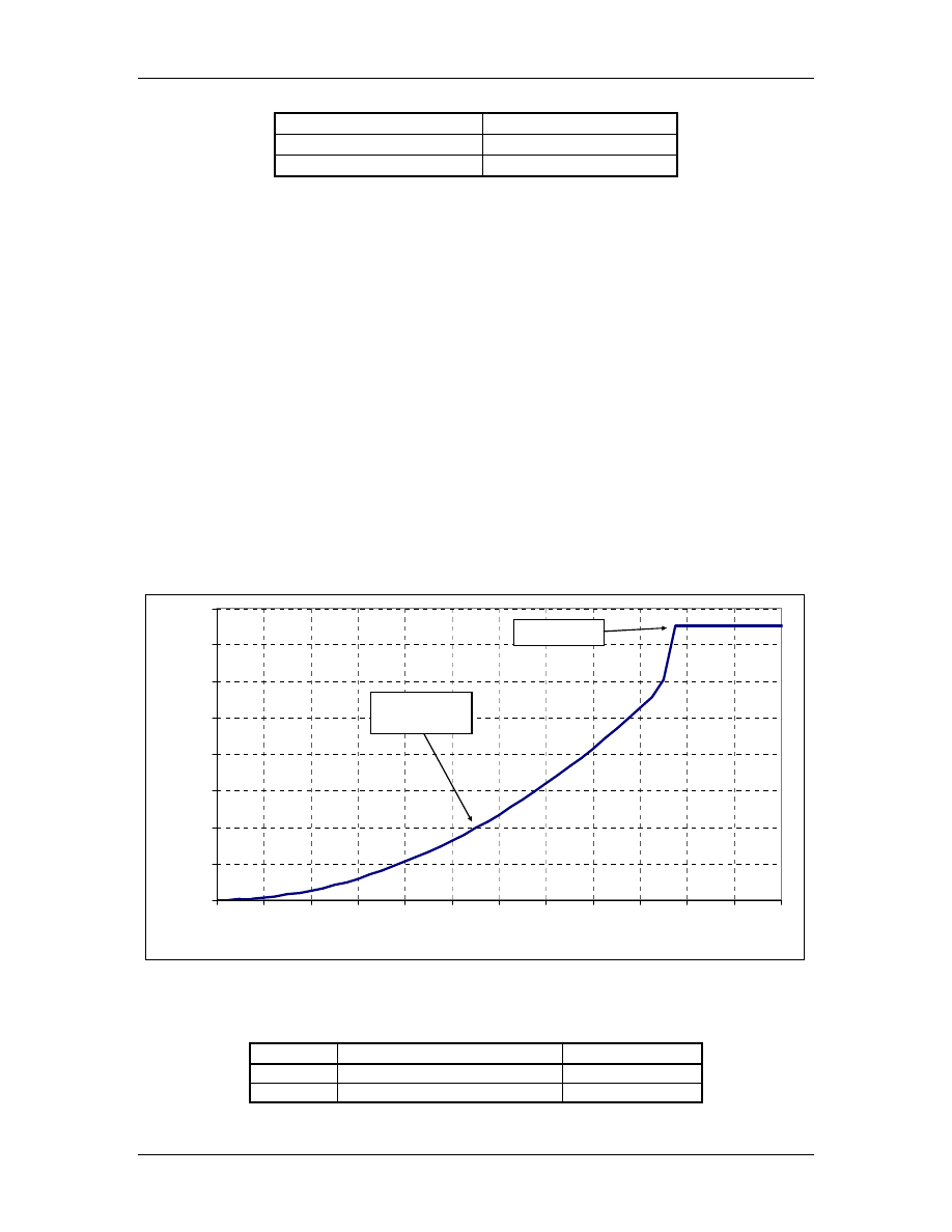
The basic control elements include the generator torque and blade pitch. Internal to the

ADAMS model, the generator is modeled with a torque versus rpm curve, and the blade

pitch actuator is modeled with a proportional-integral-derivative (PID) control loop on

the pitch command. The torque speed curve is designed to provide variable-speed

operation such that the tip speed ratio is held constant at the optimum design value, with

torque limiting once rated power is reached. This curve is shown in Figure 3.

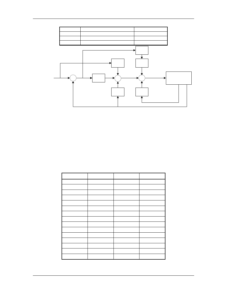
The pitch motor controller calculates a required blade pitch torque based on the pitch

command and the measured pitch and pitch rates as shown in Table 3 and Figure 4. The

structure and the gains shown are intended to result in a first-order response with time

constant tau. It is assumed that the demanded pitch rate can be approximated by the pitch

error divided by tau. The blade inertia about the pitching axis is denoted as J.

The pitch command can originate from the turbine controller, which can be either a PID

or a state space controller. The pitch of the three blades can either be coupled or

independent.

100

200

300

400

500

600

700

800

Rotor RPM

Hold constant
tip speed ratio

Torque limit

Figure 3. Generator torque speed curve

Table 3. Blade Pitch Actuator Control Gains

Term

Description

Value

Tau

Pitch response time constant

0.2 sec

Integral gain

2J/tau

RDF Project CW02

Final Report

Global Energy Concepts, LLC

October 1, 2003

Proportional gain

4J/tau

Proportional gain

2J/tau

Derivative gain

3J/tau

Derivative gain

J/tau

Pitch

Torque

Pitch

Command

Blade Pitch

Measurement

Turbine Model

Pitch

Error

K1/s

Pitch Rate

Measurement

1/tau

+-+

Figure 4. Blade pitch actuator controller block diagram

2.2.3 Aerodynamics

The aerodynamic design is based on the NREL S818/S825/S826 series airfoils. The

basic aerodynamic and geometric properties are summarized in Table 4. For this work

ADAMS version 12.0 coupled with Aerodyn [10] version 12.35 has been used. The

Aerodyn routines have been run using the equilibrium wake model with dynamic stall

turned off.

Table 4. Model Aerodynamic Section Properties

Radius, m Chord, m

Twist, deg

Airfoil

2.100

1.910

32.0

Cylinder

4.393

1.959

20.8

S818

7.543

2.063

9.6

S818

9.836

2.040

8.9

S818

12.069

1.918

7.2

S818

14.363

1.793

5.2

S818

16.505

1.679

3.1

S818

18.797

1.556

1.9

S818

21.242

1.424

1.5

S825

23.534

1.300

1.0

S825

25.466

1.196

0.6

S825

27.759

1.072

0.4

S825

30.413

0.928

0.3

S825

32.707

0.803

0.1

S826

34.426

0.710

0.0

S826

RDF Project CW02

Final Report

Global Energy Concepts, LLC

October 1, 2003

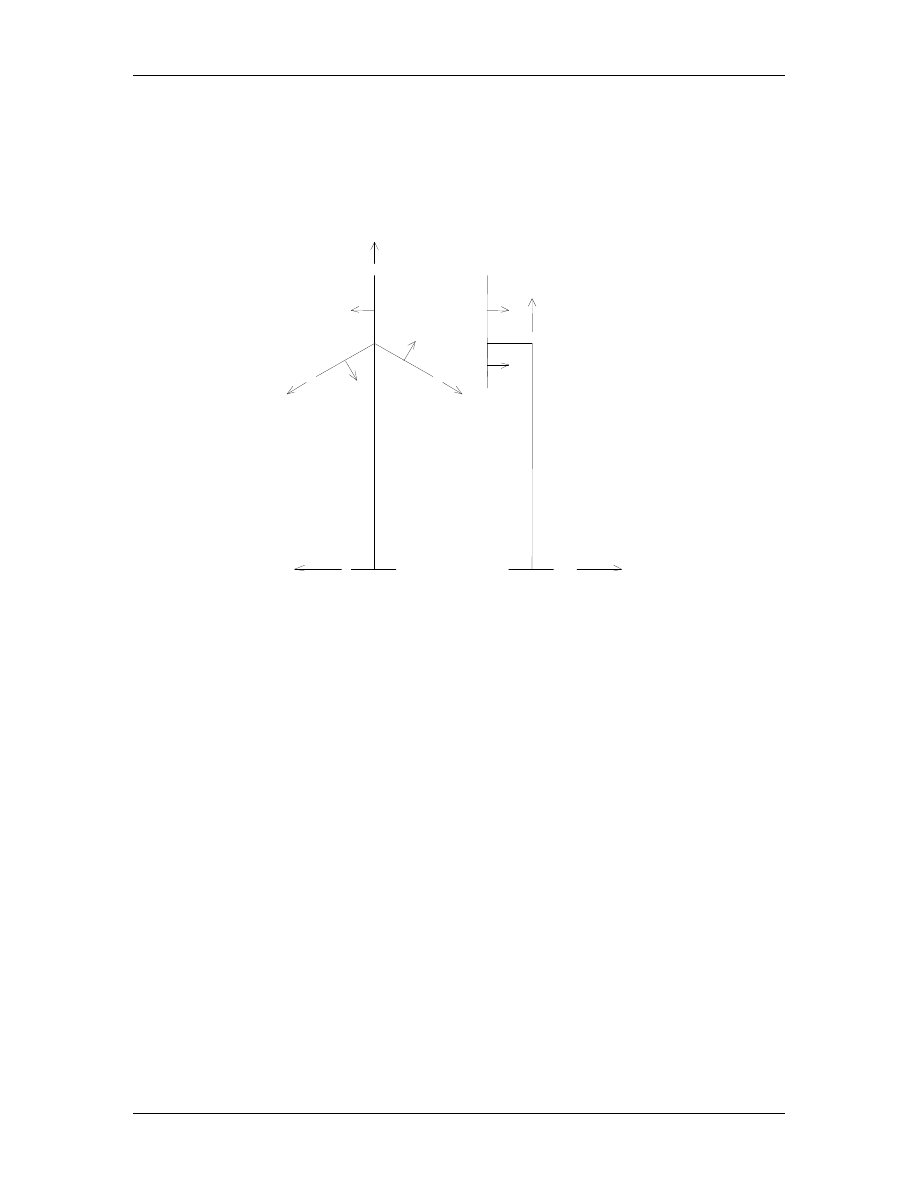
2.2.4 Coordinate Systems

The coordinate systems used throughout are based on the standard in the wind industry.

The global and individual blade fixed coordinate systems are shown in Figure 5.

Figure 5. Global (X,Y,Z) and blade (x,y,z) coordinate systems

The theoretical development uses the Coleman multi-blade transformation [11,12,13,14]

extensively. This transformation converts the blade motions from the three independent

blade fixed coordinate systems (x,y,z)

1,2,3

into one fixed-frame coordinate system

(x,y,z)

0,S,C

. The fixed-frame system will be referred to as Coleman coordinates and

consist of a symmetrical coordinate, 0; a sine (or yaw) coordinate, S; and a cosine (or tilt)

coordinate, C. While the three blade coordinate systems are used to describe the

deflections of each blade individually as seen in the rotating frame of reference, the

Coleman coordinates describe the deflections of the rotor as a whole as seen from the

fixed frame.

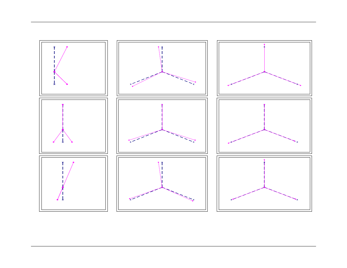
The symmetrical term is relatively easy to conceptualize. In the x direction, it refers to

collective displacement of the rotor in the upwind/downwind direction. In the y

direction, it refers to a rotation about the hub, and in the z direction it refers to a radial

stretching or shrinking of all of the blades together. The other directions are more

difficult to conceptualize. Figure 6 through Figure 8 depict the rotor displaced in each of

the nine Coleman coordinates/directions. These are shown as if the hub is fixed and the

blade tips are displaced.

RDF Project CW02

Final Report

Global Energy Concepts, LLC

October 1, 2003

Figure 6. Coleman X displacements

a) symmetrical b) sine c) cosine

Figure 7. Coleman Y displacements

a) symmetrical b) sine c) cosine

Figure 8. Coleman Z displacements

a) symmetrical b) sine c) cosine

RDF Project CW02

Final Report

Global Energy Concepts, LLC

October 1, 2003

2.3 Linearization

2.3.1 Background

The wind turbine model described above is simulated in ADAMS with a set of mixed

nonlinear differential and algebraic equations. These are coupled with the aerodynamic

forces from the Aerodyn subroutines which also exhibit nonlinear behavior. In order to

design a controller that can be coupled with the model and eventually used with a real

turbine, the nonlinear behavior must be linearized around one or more operating points of

the turbine.

Typically, analytical models used for modern control system design are linear time

invariant (LTI) state space models consisting of a set of first-order linear differential

equations. This LTI model describes the linear behavior of a dynamic physical system

around an operating point. The model includes a set of states, inputs to and outputs from

the system.

An LTI model is constructed with state variables in a vector

x(t). These variables are

usually the positions and velocities of the masses in a spring-mass-damper type of

system. The most common state variables for a wind turbine are the displacements and

velocities of points along the tower, blades, drive train, etc. These variables are related in

a linear dynamic system through a set of coupled first-order differential equations.

External forces, both a control vector u and a disturbance vector u

, affect the system.

For a wind turbine, the elements of the control vector can be individual pitch demands for

each of the blades and the generator torque demand.

These differential equations make up a state space description of a linear system and can

be expressed in matrix notation as follows:

)

(

)

Ax(

)

(

where A is a matrix containing the coefficients of the differential equations, and B

and

are the control and disturbance input influence matrices respectively.

A system that has sensors will produce measurements in a vector m that can be

analytically described as a linear combination of the states.

)

Cx(

)

where C is the state to measurement operator. Typical measurements would include

blade pitch, rpm, power, and tower top acceleration or velocity. More sophisticated

systems are being investigated for wind turbines that include blade load sensors as well.

For an operating wind turbine, a linearized model would include the structural dynamics

as well as the coupling between structural motions and the aerodynamics. A generic set

of states, inputs, and outputs for the ADAMS wind turbine model are described in Table

5 through Table 7. Note that the inputs are classified as either control or disturbance.

RDF Project CW02

Final Report

Global Energy Concepts, LLC

October 1, 2003

This corresponds to the notation u and u

used above. The outputs are also classified by

purpose. A real wind turbine only has the capability to “output” a selected number of

signals. These are indicated as “typical measurement” in Table 7. For model checkout

and control design purposes, the state space model created may also have as outputs a

number of other variables. These are required to be linear combinations of the states.

Table 5. Linearized Model States

Rotor rpm

Rotor Azimuth

Generator rpm

Generator Azimuth

Tower Elements: x,y,z,r

Displacement and

Velocity of each inertial part

Blade Pitch Angle and Rate (3 blades)

Pitch Actuator States

Blade Elements: x,y,z,r

Displacement and

Velocity of each inertial part on all 3 blades

Table 6. Linearized Model Inputs

Description

Classification

Blade pitch demand (3 blades)

Control

Generator torque

Control

Wind speed

Disturbance

Table 7. Linearized Model Outputs

Description

Purpose

Rotor rpm Typical measurement, model checking, control design

Blade pitch Typical measurement, model checking, control design

Power output Typical measurement, model checking, control design

Blade 1 out of plane displacement Model checking

Blade 1 out of plane velocity Control design

Blade 2 out of plane displacement Model checking

Blade 2 out of plane velocity Control design

Blade 3 out of plane displacement Model checking

Blade 3 out of plane velocity Control design

Tower fore-aft displacement Model checking

Tower fore-aft velocity Typical measurement, control design

Shaft torsional deflection Model checking

Shaft torsional deflection velocity Control design

RDF Project CW02

Final Report

Global Energy Concepts, LLC

October 1, 2003

2.3.2 ADAMS Linear

An add-on linearization option is available for the standard ADAMS software. This

option will provide the A, B, C, and D matrices for an LTI model around a specific

operating point. While the ADAMS linearization procedure is applicable to a broad class

of physical models, the user’s manual cautions against linearizing models that have parts

rotating about axes not passing through the center of mass. The example given is of a

structure with articulated outboard parts spinning around a central hub, essentially the

definition of a wind turbine. The problem is that when ADAMS freezes the model for

linearization, it preserves instantaneous velocities, but does not preserve the presence of

the rotational constraint. The resulting linearized model does not properly contain the

forces that arise due to rotation, namely the centrifugal and gyroscopic forces. These

rotational effects can be of considerable importance to wind turbine structural dynamic

response.

Another difficulty is associated with the aerodynamic subroutines. ADAMS linear will

include the effects of forces calculated in subroutines, but unless the functions are smooth

and continuous, difficulties can arise. The Aerodyn subroutines meet this criterion in a

broad sense, adequate for the time step simulations. However, when changes to the

inputs become small (as they do during the linearization process) the results are not

reliable.

2.3.3 Aerodynamic Linearization

The issue of the aerodynamic derivatives is relatively easy to address. ADAMS provides

a high degree of control over both the “operation” of the turbine model and the output of

results. This capability can be exercised to provide numerical results corresponding to

the effects of perturbations on the aerodynamic forces at each blade element.

Considerable effort was put into understanding the interaction between ADAMS and

Aerodyn. This included discussions with ADAMS technical support as well as

experimentation with the simulations. The ADAMS linearization process is essentially to

evaluate the Jacobian matrix of the model at the current operating point. For force

subroutines such as Aerodyn, the partial derivatives of these forces with respect to all of

the pertinent state variables are required. To get these derivatives, ADAMS calls the

subroutines and passes to them values for the state variables that have been slightly

perturbed. Variables are perturbed one state at a time, with the perturbations at the part

center of mass in the global coordinate system. All state variables in the subroutine from

parts not currently being perturbed do not change their value.

Detailed experimentation with and review of these calculations, has shown that the state

variable perturbations sent to Aerodyn by ADAMS are very small. For a force

subroutine that contains a closed-form analytical expression, this will most likely result in

force calculations and resulting partial derivatives that are well behaved. Unfortunately

the Aerodyn subroutines are complex, and since the equations are not in a closed form,

convergence of an iterative solution is required. They also rely on lookup tables for

aerodynamic lift and drag calculations. As a result, it appears that without the

RDF Project CW02

Final Report

Global Energy Concepts, LLC

October 1, 2003

considerable effort of reworking the Aerodyn subroutines, they are unsuitable for this

task as currently realized.

A solution to this problem has been conceived and implemented, however. It is clear for

which of the state variables and model inputs the partial derivatives of aerodynamic force

must be calculated. These are the velocities of the blade elements relative to ground, the

overall rotation of the blade element about the pitch axis (rigid body pitch plus torsional

flexing) and the wind inflow input. A process has been developed to calculate the

derivatives of the aerodynamic forces around a selected operating point with respect to

these variables. These derivatives are then used in an aerodynamic subroutine

specifically written for the ADAMS linearization procedure.

The following is a basic procedural outline of the process:

• The model is set up in such a way as to obtain the highest quality results. This

includes turning off gravity to avoid once-per-rev oscillations, increasing the

structural damping properties of the blades to minimize other oscillations, and

putting the nacelle on a rigid tower to avoid the secondary effect of the tower

tilting back in the flow field.

• The base of the rigid tower is also mounted on a translational joint relative to

ground. This allows for control of the rotor velocity in the upwind/downwind

direction. Note that the aerodynamics calculations treat wind velocity and

velocity due to motion of the blades differently.

• The turbine is run at a steady-state condition and each of four variables is stepped

slightly to either side of nominal, one at a time. Table 8 shows these variables

and a typical step size.

• A time series of the forces and variables shown in Table 9 is saved for each blade

element from all three blades.

• The one variable that cannot be precisely controlled is the blade element torsional

deflection because it varies as the aerodynamic forces cause overall blade

deflections. These forces and deflections change as each of the listed global

variables is perturbed. As a result, there is coupling in the results and the

derivatives cannot be calculated individually.

• A least-squares approach is used to solve this problem. Specifically, the pseudo

inverse function in Matlab is used on the set of equations obtained from the time

series data for each blade element to solve for the partial derivatives:

∂

∆

(1)

where n is the number of time steps in the time series.

RDF Project CW02

Final Report

Global Energy Concepts, LLC

October 1, 2003

• This is repeated for Fx and Fy in blade coordinates and the results for the three

blades are averaged for each aerodynamic derivative at each blade element. The

matrix of results is saved to a file which can be read by the subroutine linked to

the ADAMS linearization procedure.

Table 8. Perturbations for Aerodynamic Derivative Calculation

Global Variable

Perturbation

Collective blade pitch angle

±0.5 degrees

Wind speed

±0.5 m/s

Rotor rpm

±0.5 rpm

Tower upwind/downwind

velocity

±0.5 m/s

Table 9. Aerodynamic Derivatives

Blade Element Variable

Normal Force, Fx

Tangential Force, Fy

Element torsional deflection

plus pitch,

δFx/δφ

δFy/δφ

Wind speed, V

δFx/δV

δFy/δV

Element tangential velocity v

δFx/δv

δFy/δv

Element normal velocity, v

δFx/δv

δFy/δv

2.3.4 Linearization of Rotational Effects

The inclusion of the rotational effects is more problematic. However, a methodology was

developed that can produce an accurate linear time invariant model of an operating wind

turbine at a stable operating point. The crux of this methodology is the conversion of the

equations of motion from state variables in the rotating frame to a set of state variables in

the fixed frame. This conversion removes the time varying terms from the equations of

motion. The rotationally induced forces are identified in these equations and used in a

subroutine linked to ADAMS. Figure 9 outlines the methodology that will be developed

in detail in the following sections.

RDF Project CW02

Final Report

Global Energy Concepts, LLC

October 1, 2003

Develop equations of motion for a
blade part flexibly connected to a
rotating hub in blade coordinates

Convert these equations to the
fixed frame using the Coleman
transformation - assuming the rotor
azimuth angle varies in time

Convert above result back to blade
coordinates using the Coleman
transformation - assuming the rotor
azimuth angle is fixed

Extract equations for forces
dependent on rotation rate from
above EOM and code into
ADAMS subroutine

Sum terms from EOM and the aero
forces dependent on blade
velocities into state coefficient
matrix

Form the matrix of partial derivatives
relating the aerodynamic forces to the
blade velocities, pitch angle, and wind
speed

These equations show uncoupled
blade motions, however the state
coefficient matrix is time
dependent

These equations show coupling between the fixed frame displacements,
however the state coefficient matrix is no longer time dependent.
It is also noted that aerodynamic terms are present as coefficients of the
displacements as well as the velocities

This step preserves the coupling
between blade motions as well as the
aerodynamic terms that act on the
displacements

ADAMS model of wind turbine - static
solution with no applied forces and no
rotation

Linearize model of wind turbine -
blade state perturbations used to
calculate perturbed values of
aerodynamic and rotationally
induced forces

Select an operating point: wind
speed, RPM, pitch angle

Figure 9. Outline of methodology for linearization of rotational effects

RDF Project CW02

Final Report

Global Energy Concepts, LLC

October 1, 2003

2.3.4.1 Equations of Motion

The approach requires equations for the forces that act on a blade inertial element when

its states are perturbed. These forces can then be applied to the non-rotating turbine

model during the linearization process through a custom force subroutine. A static

solution is first computed for the non-rotating model. The ADAMS linear procedure then

perturbs the model states to evaluate the Jacobian, and as part of this process the

rotational and aerodynamic forces due to these perturbations are calculated and returned

by the subroutine.

The development of the theoretical basis for this subroutine hinges on the use of a multi-

blade transformation used for analysis of helicopter and wind turbine rotor dynamics

[11,12,13,14], referred to as a Coleman transformation in this report. This transformation

between the translational displacements in blade fixed coordinates and a set of non-

rotating coordinates is expressed as follows for three identical points on each of the three

blades. Also included are the hub coordinates in a global frame of reference.

[ ]

where

, and

cos

sin

cos

sin

cos

sin

(2)

I is the identity matrix with a dimension of 3 and

)

(

−

Ω

is the azimuth angle of blade i relative to blade 1 vertically upwards. The blade and

fixed-frame displacement vectors for blade #i to fixed coordinate #j are organized as:

i = 1,2,3,h and

j = 0,S,C,h

(3)

The fixed-frame coordinates x

, x

, and x

, are a set of coordinates that represent the

symmetric, sine (or yaw), and cosine (or tilt) components of the displacement in the non-

rotating frame of reference.

From Malcolm [13], the equations of motion for the three translational degrees of

freedom of three identical inertial elements on the three blades plus the hub are as

follows, ignoring the effects of element rotations:

RDF Project CW02

Final Report

Global Energy Concepts, LLC

October 1, 2003

−

Ω

−

Ω

)

(

)

(

)

(

)

(

)

(

)

(

aero

(4)

where X

is the X

displacement vector, m

and m

are the masses of a single blade

element and the hub, respectively,

Ω is the rotor rotation rate, and F

aero

is the applied

aerodynamic loading. The blades are connected individually to the hub through the block

diagonal stiffness matrix K

and the hub is attached to ground through stiffness matrix

. C and S are block diagonal matrices with three blocks each of the form:

−

and

(5)

L is a matrix that transforms global coordinates into blade coordinates with three

elements vertically stacked of the form:

−

)

(

cos

)

(

sin

)

(

sin

)

(

cos

(6)

It is this term in the equations of motion for the rotor that is time variant. The following

analysis will remove this time dependency by using the Coleman transform.

2.3.4.2 Aerodynamic Forces

It is known that the aerodynamic forces are dependent on the wind speed, the blade pitch,

and the blade element velocities. The applied force in Eq. (4) can be expressed as

follows:

aero

with

∆

i=1,2,3 for the three blades

(7)

where D is the block diagonal matrix

with

δφ

(8)

RDF Project CW02

Final Report

Global Energy Concepts, LLC

October 1, 2003

and

and V

are the pitch and wind speed at blade i. Note that

and

, the radial

aerodynamic force and radial blade part velocity are both typically assumed to be zero.

Substitute Eq. (7) and Eq. (8) into Eq. (4) and collecting terms of

, and

yields:

−

Ω

−

Ω

)

(

)

(

)

(

)

(

)

(

)

(

)

(

(9)

where U now only contains the pitch and wind speed of the three blades and D

and D

are block diagonal.

2.3.4.3 Conversion to Fixed Frame

It is now necessary to convert Eq. (9) into the fixed frame in order to remove the time

dependent term embodied in L. Note that Eq. (9) is composed of three uncoupled blocks,

one for each blade, plus the hub. These equations can be transformed into the fixed-

frame Coleman coordinates via use of the relationships given in Hansen [14] for the

derivatives and inverse of B, the transformation matrix of Eq. (2):

and

−1

with

(10)

Ω

−

and

(11)

With X=BZ

taking derivatives using Eqs. (10 and 11) yields:

BRZ

and

(12)

These can be substituted into Eq. (9) and rearranged to give:

−

)

(

(13)

where A is the coefficient matrix of Eq. (9) and U

are the inputs transformed to Coleman

coordinates with a B matrix of the appropriate dimension.

RDF Project CW02

Final Report

Global Energy Concepts, LLC

October 1, 2003

A calculation was carried out using a symbolic math package to put Eq. (13) into a

standard form in the Coleman coordinates, Z. The result is as follows:

)

(

(14)

where

−

Ω

−

Ω

−

Ω

−

Ω

)

(

)

(

)

(

)

)(

(

)

(

)

(

)

(

)

(

)

(

)

(

)

(

)

(

)

)(

(

)

(

(15)

and

Ω

−

Ω

−

Ω

−

Ω

−

)

(

)

(

)

(

(16)

The significance of Eqs. (14-16) is that the time variant system with no blade coupling in

the rotating frame has been converted to a time invariant system with coupling between

the blades in the fixed frame. Also of importance is that the aerodynamic derivatives

embodied in D

from Eq. (8) become coefficients of the displacement states as well as

velocity states. Finally, it is noted that the input matrix is the same in fixed frame as it

was in blade coordinates. These are the equations that give the proper dynamics for a

rotating turbine viewed from the fixed frame. The blade part forces are implied by the

row in the matrix corresponding to the blade part accelerations with a multiplication by

the mass.

2.3.4.4 Conversion back to Blade Coordinates – fixed azimuth

The forces implied in Eq. (14) could conceivably be applied in the Coleman form to the

non-rotating model undergoing linearization. However it is more straightforward to

apply the forces in blade coordinates, as these are most easily passed in and out of the

custom subroutine.

The necessary assumption is that the equations of motion can be converted back to blade

coordinates with the azimuth angle now a constant instead of a function of time. This

removes the need to chain rule the derivatives for the transformation so that

−

and

Z =

−

(17)

RDF Project CW02

Final Report

Global Energy Concepts, LLC

October 1, 2003

Substituting Eqs. (17) into Eq. (14) yields a set of equations for the blade motions in

blade coordinates for a rotor that is instantaneously stationary:

)

(

(18)

where the hub terms have been removed. For convenience, define:

−

and

−

(19)

So that

)

)(

(

)

(

)

(

)

(

Ω

−

and

[

]

Ω

−

)

(

)

(

(20)

This result preserves the coupling between the blade motions as well as the coupling of

the aerodynamics to the displacements. The forces due to rotation are the terms in A

and

that contain the rotor speed,

Ω , multiplied by the blade part mass. They are extracted

and expressed as follows:

Ω

)

(

(21)

where

−

(22)

and

RDF Project CW02

Final Report

Global Energy Concepts, LLC

October 1, 2003

−

(23)

The ADAMS linearization procedure views the rotor as stationary, as this is a necessary

condition for the core procedure to give accurate results. The custom subroutines apply

forces to that stationary rotor is if it were actually rotating. In particular, when ADAMS

perturbs the states for the linearization calculation, the custom subroutine returns the

forces that would arise from those perturbations as if the rotor were rotating.

2.3.4.5 Pitch Actuator

The independent blade pitch actuators are modeled with PID loops from pitch demand to

pitching torque, one for each blade. These PID loops are built in to the ADAMS model

and get linearized as part of the overall plant. When testing the method, a problem arose

wherein the full ADAMS model response to a step in Coleman sine or cosine pitch angle

demand showed some steady state coupling, particularly when the pitch actuator time

constant was long.

A Coleman sine or cosine demand in pitch looks like steady state in the fixed frame,

however in the blade frame of reference this looks like a sinusoidally varying demand.

Due to following error, the lag in response looks like steady state coupling between the

sine and cosine components of the pitch angle. The rotating turbine must continually

pitch the blades at once per revolution to maintain a sine or cosine pitch angle in the fixed

frame. The following error of the actuator results in steady state coupling.

The linearized model shows a response to these step changes in demand with no steady

state coupling. The linear model does not have the following error, as the blades are not

rotating and the pitch actuator does not cycle at once per revolution.

To address this issue, an approach similar to the operations in the above section is

developed where the equations of motion are developed and transformed to the fixed

frame in Coleman coordinates. The closed loop equations of motion for the pitch of three

rigid blades can be expressed as follows, referring to the description of the actuator in

Figure 4 and Table 3:

( )

−

)

)(

(

)

(

)

(

)

)(

(

(24)

where

φ is a vector of the three blade pitch angles, the subscripts I and d denote the

integral of the pitch error and the pitch demand respectively. The 0 and I refer to three by

three matrices of zeros and the identity matrix respectively. J is the blade pitch inertia.

RDF Project CW02

Final Report

Global Energy Concepts, LLC

October 1, 2003

When this set of equations is transformed using the Coleman transformation matrix B to

the fixed frame and then transformed back to blade coordinates with an assumption of an

instantaneously non-rotating rotor, the result in blade coordinates is:

[

]

( )

Ω

−

Ω

)

)(

(

)

(

)

(

)

(

)

(

)

(

)

(

)

(

)

(

(25)

where

−

and

−

(26)

The additional terms in this coupled set of equations are noted to all be dependent on the

rotor speed,

Ω . These additional terms are coded into the blade pitch actuator used in

the ADAMS model of the stationary rotor.

2.3.4.6 Implementation Issues

Application of this methodology to a fully complex ADAMS model of a wind turbine

highlighted a few issues that should be noted.

• The procedure performs more reliably when symmetry is maintained in the rotor

model. This requires that the definition of the blade part locations be made with a

high degree of accuracy.

• For the rotational force calculations, many of the states required are essentially

velocities of the blade part centers of mass. It was found to be important to

superimpose a marker in the fixed frame at the location of each blade part center

of mass from which to calculate the velocity.

RDF Project CW02

Final Report

Global Energy Concepts, LLC

October 1, 2003

3 Validation and Results

3.1 Response Calculations

One attribute of a linearized model is that it should duplicate the behavior of the non-

linear model in the neighborhood of a selected operating point. In order to validate the

methodology developed in the previous section, the approach will be to compare the

results from simulations using the linearized model to results from the simulation using

the full non-linear ADAMS model. The linearized model simulations are carried out in

MATLAB using the step function. The step function applies unit steps individually to

each of the inputs to an LTI model and calculates the states and outputs for each.

The LTI model used for these examples uses inputs and outputs that are defined in terms

of the Coleman coordinates, with the exception of the shaft torque and tower motion.

The blade pitch demand inputs and the wind inputs are both expressed in Coleman

coordinates for the rotational and downwind directions, respectively. The blade pitch tip

displacement outputs are also all in Coleman coordinates. The full non-linear ADAMS

model inputs and outputs have also been converted by applying the inverse of the

transformation in Equation 2.

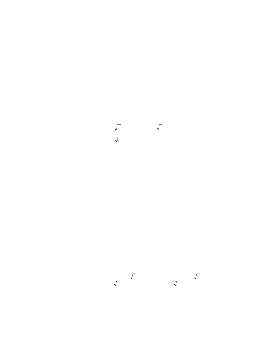
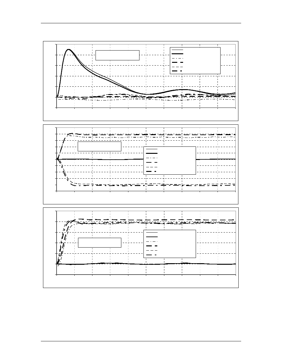
The comparison for the blade pitch response is shown in Figure 10. Note that the

response to a collective pitch demand matches exactly and that there are no coupled

motions in the sine and cosine directions. The response to sine and cosine pitch demands

produces a coupled response from the LTI model that matches the non-linear model fairly

well. The discrepancies are most likely due to effects that are not included in the linear

model, such as the deflection of the blade operating in high wind speeds in the full model.

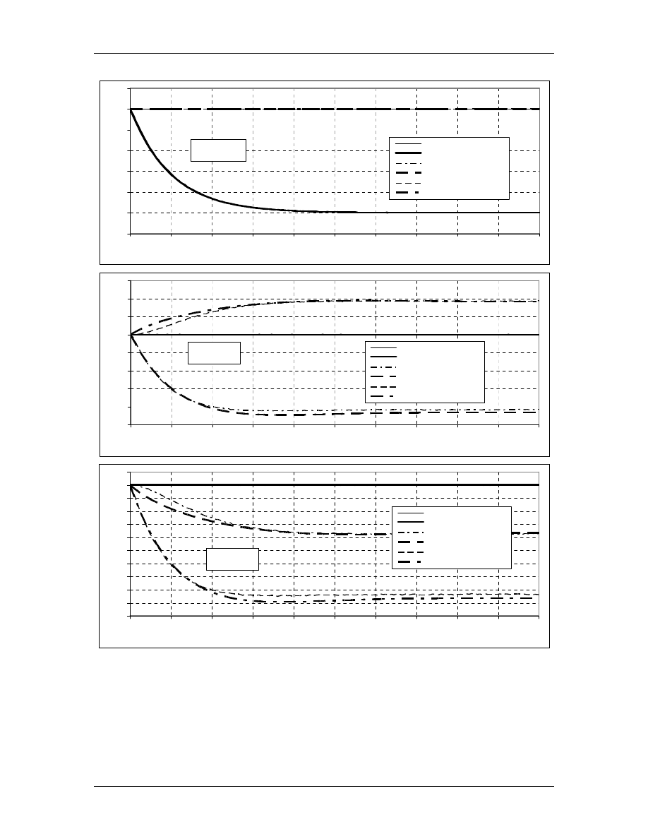
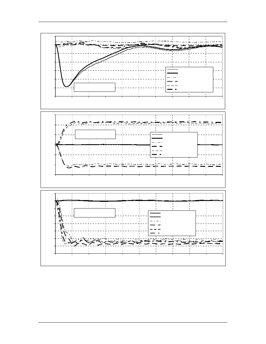
The response of the turbine rotor speed and the tower motion to step changes in blade

symmetric pitch, wind speed, and generator torque is shown in Figure 11. These show

quite good comparisons for the rpm. The tower motion results are not as good; however,

oscillations in the tower motion from the full model were present before the step change,

making them difficult to compare.

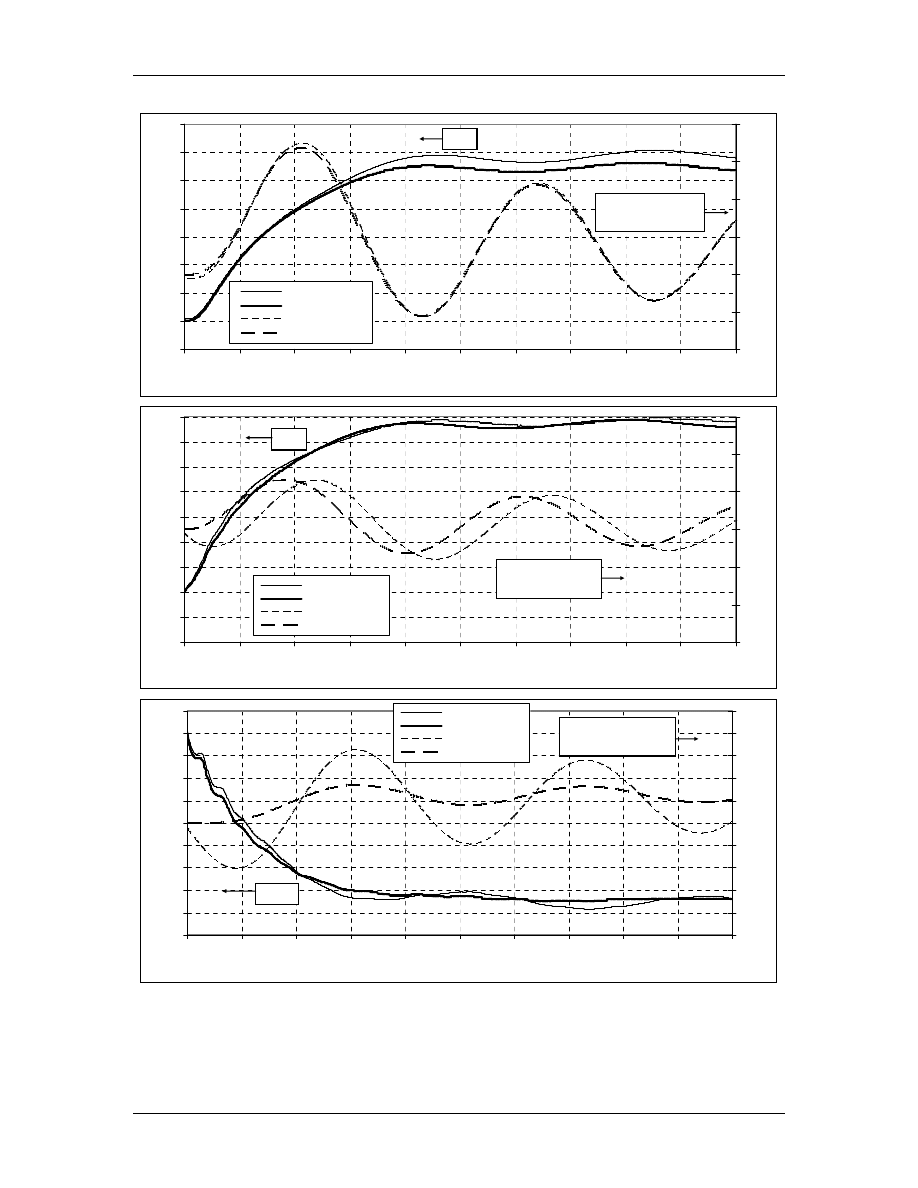
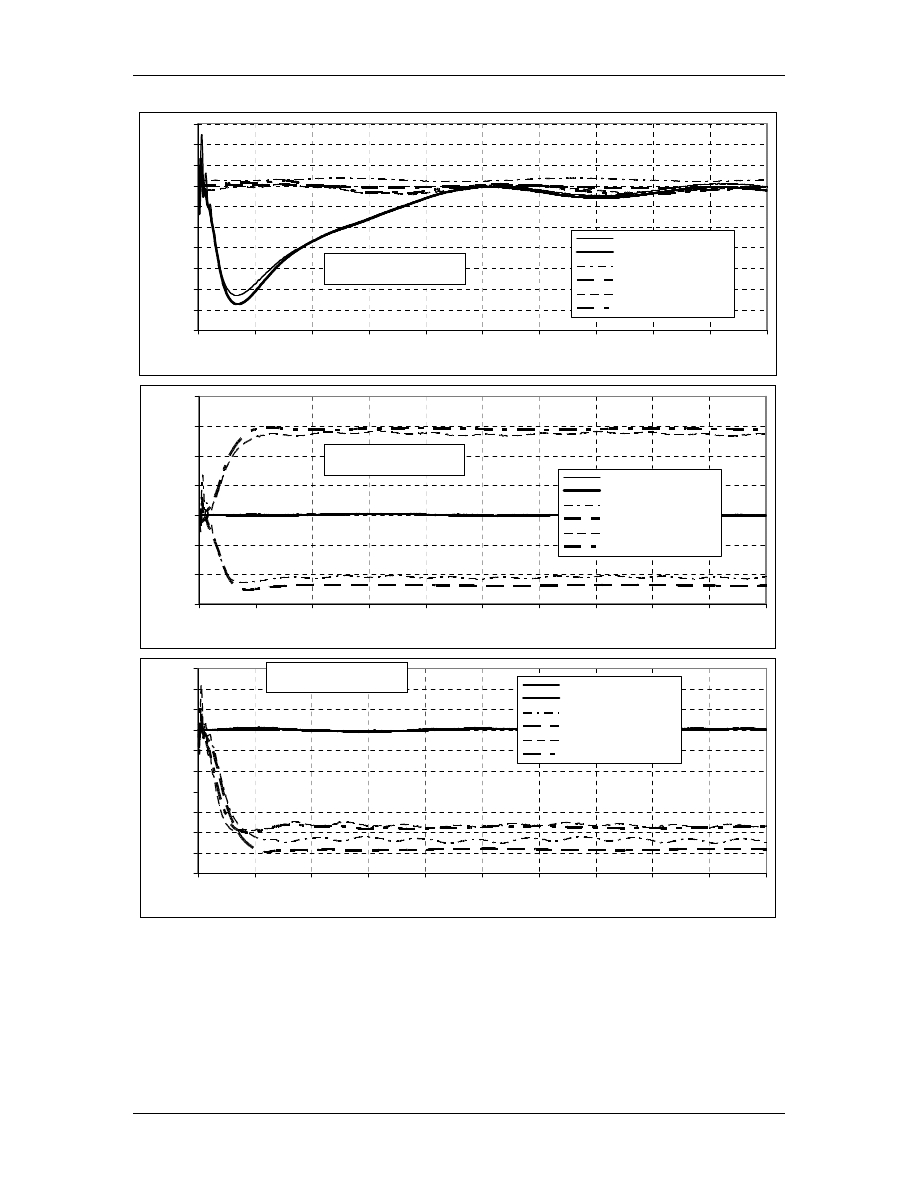
The response of blade tip deflections to step changes in the Coleman pitch demand inputs

are shown in Figure 12 to Figure 14. These include deflections in the x, y and blade

torsional directions.

RDF Project CW02

Final Report

Global Energy Concepts, LLC

October 1, 2003

-1.2

-1.0

-0.8

-0.6

-0.4

-0.2

0.0

0.2

40.0

40.2

40.4

40.6

40.8

41.0

41.2

41.4

41.6

41.8

42.0

Time, seconds

ADAMS - Collective

Matlab - Collective

ADAMS Sin

Matlab Sin

ADAMS Cos

Matlab Cos

Blade Pitch,
deg

-1.0

-0.8

-0.6

-0.4

-0.2

0.0

0.2

0.4

0.6

40.0

40.2

40.4

40.6

40.8

41.0

41.2

41.4

41.6

41.8

42.0

Time, seconds

ADAMS - Collective

Matlab - Collective

ADAMS Sin

Matlab Sin

ADAMS Cos

Matlab Cos

Blade
Pitch, deg

-1.0

-0.9

-0.8

-0.7

-0.6

-0.5

-0.4

-0.3

-0.2

-0.1

0.0

0.1

40.0

40.2

40.4

40.6

40.8

41.0

41.2

41.4

41.6

41.8

42.0

Time, seconds

ADAMS - Collective

Matlab - Collective

ADAMS Sin

Matlab Sin

ADAMS Cos

Matlab Cos

Blade
Pitch, deg

Figure 10. Response of the blade pitch to a step change in: a) symmetrical b)

sine c) cosine pitch demand while operating in steady 24 m/s winds

RDF Project CW02

Final Report

Global Energy Concepts, LLC

October 1, 2003

-0.2

0.0

0.2

0.4

0.6

0.8

1.0

1.2

1.4

Time, seconds

-0.04

-0.02

0.00

0.02

0.04

0.06

0.08

ADAMS RPM

Matlab RPM

ADAMS Twr

Matlab Twr

RPM

Tower Top fore-aft
Displacement, m

-0.4

-0.2

0.0

0.2

0.4

0.6

0.8

1.0

1.2

1.4

Time, seconds

-0.15

-0.10

-0.05

0.00

0.05

0.10

0.15

ADAMS RPM

Matlab RPM

ADAMS Twr

Matlab Twr

RPM

Tower top fore-aft
displacement, m

-0.9

-0.8

-0.7

-0.6

-0.5

-0.4

-0.3

-0.2

-0.1

0.0

0.1

Time, seconds

-0.10

-0.08

-0.06

-0.04

-0.02

0.00

0.02

0.04

0.06

0.08

0.10

ADAMS RPM

Matlab RPM

ADAMS Twr

Matlab Twr

RPM

Tower top fore-aft
displacement, m

Figure 11. Response of rotor rpm and tower motion to a step change in:

a) symmetrical pitch demand b) wind speed c) generator torque while operating

in steady 24 m/s winds

RDF Project CW02

Final Report

Global Energy Concepts, LLC

October 1, 2003

-0.1

0.0

0.1

0.2

0.3

Time, seconds

ADAMS - Collective

Matlab - Collective

ADAMS Sin

Matlab Sin

ADAMS Cos

Matlab Cos

Blade Tip Out of Plane
Displacement, m

-0.3

-0.2

-0.1

0.0

0.1

0.2

0.3

Time, seconds

ADAMS - Collective

Matlab - Collective

ADAMS Sin

Matlab Sin

ADAMS Cos

Matlab Cos

Blade Tip Out of Plane
Displacement, m

-0.1

0.0

0.1

0.2

0.3

Time, seconds

ADAMS - Collective

Matlab - Collective

ADAMS Sin

Matlab Sin

ADAMS Cos

Matlab Cos

Blade Tip Out of Plane
Displacement, m

Figure 12. Response of the blade tip Coleman x direction deflection to a step

change in: a) symmetrical b) sine c) cosine pitch demand while operating in

steady 24 m/s winds

RDF Project CW02

Final Report

Global Energy Concepts, LLC

October 1, 2003

-0.12

-0.10

-0.08

-0.06

-0.04

-0.02

0.00

0.02

Time, seconds

ADAMS - Collective

Matlab - Collective

ADAMS Sin

Matlab Sin

ADAMS Cos

Matlab Cos

Blade Tip In Plane
Displacement, m

-0.15

-0.10

-0.05

0.00

0.05

0.10

0.15

Time, seconds

ADAMS - Collective

Matlab - Collective

ADAMS Sin

Matlab Sin

ADAMS Cos

Matlab Cos

Blade Tip In Plane

Displacement, m

-0.14

-0.12

-0.10

-0.08

-0.06

-0.04

-0.02

0.00

0.02

Time, seconds

ADAMS - Collective

Matlab - Collective

ADAMS Sin

Matlab Sin

ADAMS Cos

Matlab Cos

Blade Tip In Plane

Displacement, m

Figure 13. Response of the blade tip Coleman y direction deflection to a step

change in: a) symmetrical b) sine c) cosine pitch demand while operating in

steady 24 m/s winds

RDF Project CW02

Final Report

Global Energy Concepts, LLC

October 1, 2003

-0.007

-0.006

-0.005

-0.004

-0.003

-0.002

-0.001

0.000

0.001

0.002

0.003

Time, seconds

ADAMS - Collective

Matlab - Collective

ADAMS Sin

Matlab Sin

ADAMS Cos

Matlab Cos

Blade Tip Torsional
Displacement, radians

-0.006

-0.004

-0.002

0.000

0.002

0.004

0.006

0.008

Time, seconds

ADAMS - Collective

Matlab - Collective

ADAMS Sin

Matlab Sin

ADAMS Cos

Matlab Cos

Blade Tip Torsional
Displacement, radians

-0.007

-0.006

-0.005

-0.004

-0.003

-0.002

-0.001

0.000

0.001

0.002

0.003

Time, seconds

ADAMS - Collective

Matlab - Collective

ADAMS Sin

Matlab Sin

ADAMS Cos

Matlab Cos

Blade Tip Torsional
Displacement, radians

Figure 14. Response of the blade tip Coleman torsional deflection to a step

change in: a) symmetrical b) sine c) cosine pitch demand while operating in

steady 24 m/s winds

RDF Project CW02

Final Report

Global Energy Concepts, LLC

October 1, 2003

3.2 Modal Analysis

Modal analysis of an operating wind turbine has always been challenging because of the

relationship between the rotor and the supporting structure. The modal analysis is highly

dependent on the rotor rotation rate as was demonstrated in Section 2. Malcolm [13] has

developed an approach that was the initial basis for this work. This work, while

primarily interested in control design tools, has extended the methodology for modal

analysis to include the aerodynamic effects. In the future, it may also be possible to

extend the methodology to include the effect of sensor dynamics and control algorithms

in the open or closed loop.

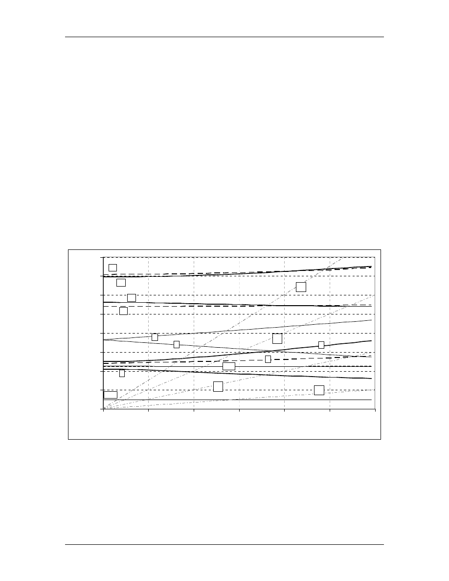
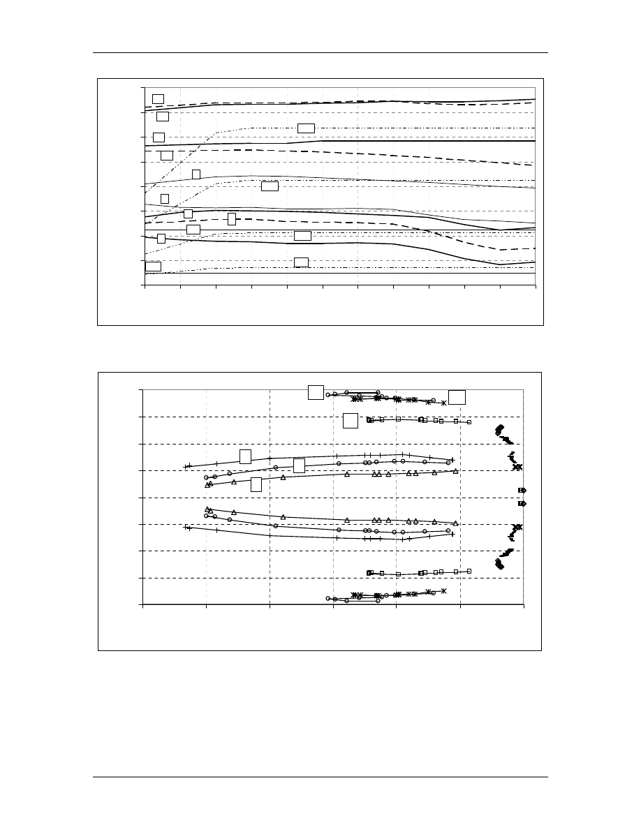
One benefit of this methodology is that Campbell diagrams can be readily produced.

Figure 15 shows a Campbell diagram for the example 1.5 MW turbine. Table 10 gives

the associated descriptions and frequencies for the modes. These results show the

expected divergence of the asymmetrical modes as the rpm increases. This divergence

produces a frequency difference between matched modes equal to twice the rotor rotation

frequency. The slight increase in frequency of the flap collective modes due to

centrifugal stiffening is also shown.

0.0

0.5

1.0

1.5

2.0

2.5

3.0

3.5

4.0

RPM

1, 2

4, 5

Figure 15. Campbell diagram for the example 1.5 MW turbine

RDF Project CW02

Final Report

Global Energy Concepts, LLC

October 1, 2003

Table 10. Modal Frequencies for Example 1.5 MW Turbine

Mode #

Description

Frequency, Hz

at 0 rpm

Frequency, Hz

at 30 rpm

Tower fore-aft

0.24

Tower lateral

0.24

Flap tilt

1.05

0.80

Tower lateral

1.10

1.11

Tower fore-aft

1.13

1.12

Flap collective

1.20

1.40

Flap yaw

1.25

1.80

Edge tilt

1.81

1.35

Edge yaw

1.83

2.34

Drive train torsion/edge

collective*

2.70

2.74

Flap yaw

2.81

2.69

flap tilt

3.47

3.73

Flap collective

3.54

3.76

* The 1

drive train mode is the rigid body rotation of the rotor and drive train

The results in Figure 15 and Table 10 were calculated using the rotational force

subroutine described in the previous section. The aerodynamic forces, however, were

turned off, and the pitch angle was held at the fine pitch set point. With the aerodynamic

force effects included and the pitch angle varied appropriately, a similar review of the

modal response can be made as a function of operating point wind speed. Eigensolutions

were calculated for steady operating points from 6 to 28 m/s in 2 m/s increments. A

Campbell diagram versus wind speed is shown in Figure 16. This shows the effects of

aerodynamic damping in high winds where many of the modal frequencies are reduced.

Plots of the loci of system poles versus wind speed are shown in Figure 17 and Figure 18.

The poles generally move from right to left with increasing wind speed. The numbered

labels in these figures correspond to Table 10. Figure 19 shows the pole loci for the rigid

body rotor and drive train rotation. Again the poles move from right to left with

increasing wind speed.

RDF Project CW02

Final Report

Global Energy Concepts, LLC

October 1, 2003

0.0

0.5

1.0

1.5

2.0

2.5

3.0

3.5

4.0

Wind Speed, m/s

1,2

4,5

9 P

6 P

3 P

1 P

Figure 16. Wind speed Campbell diagram for the example 1.5 MW turbine

-4

-3

-2

-1

-12

-10

-8

-6

-4

-2

Real

Figure 17. System pole loci for the example 1.5 MW turbine

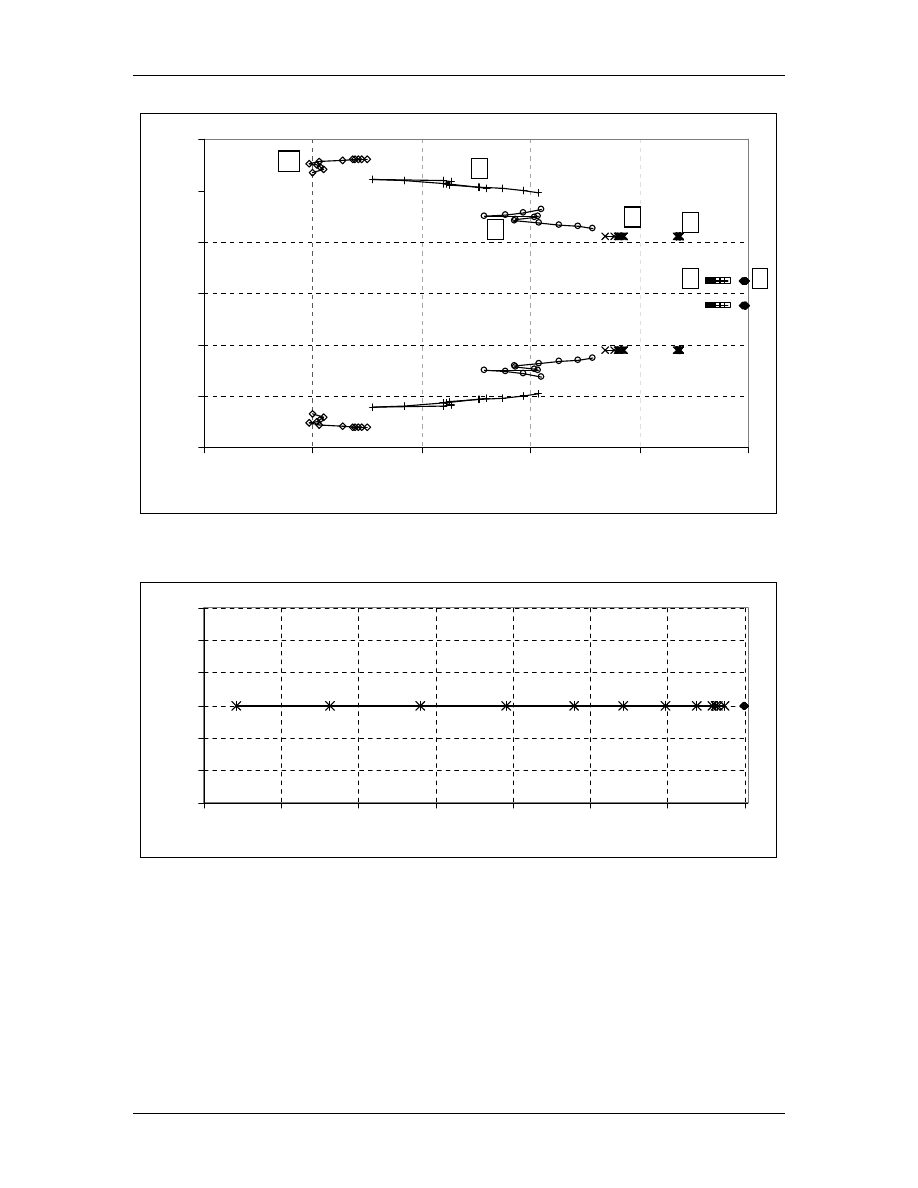
RDF Project CW02

Final Report

Global Energy Concepts, LLC

October 1, 2003

-3

-2

-1

-1.0

-0.8

-0.6

-0.4

-0.2

0.0

Real

Figure 18. System pole loci for the example 1.5 MW turbine

-3

-2

-1

-1.4

-1.2

-1.0

-0.8

-0.6

-0.4

-0.2

0.0

Real

Figure 19. Pole loci for the rotor and drive train rigid body rotation

RDF Project CW02

Final Report

Global Energy Concepts, LLC

October 1, 2003

3.3 Controls

3.3.1 Model Reduction

Once an LTI is available, it can be imported into Matlab for control design. The first

issue that arose using a linear model of a complex turbine ADAMS model is that there

are on the order of 300 displacement degrees of freedom. This is far too many to do a

practical control design. There are a variety of approaches to reducing the model order

down to a manageable level without losing important information.

One of the most straightforward of these methods is to convert the LTI model into modal

form and pick out the most important modes for use in a reduced order model. The work

presented in the above section was critical to carrying out this reduction. Table 11 shows

the modes kept for a model linearized around an operating point at 24 m/s. With these

modes included, the fidelity of the rpm, tower motion, and blade flapping motion

response to symmetric pitch and wind input remains intact.

Table 11. Modes Included for a Reduced Order Model

Mode # Description

Frequency, Hz

Real part of

Eigenvalue

Drive train rigid body

0.00

-0.84

Collective pitch actuation

0.00

-5.00

Tower fore-aft

0.24

-0.07

Flap collective

0.87

-9.28

Drive train torsion

2.52

-1.64

3.3.2 State Feedback and Kalman Filtering

The control design example to follow makes use of standard state space control design

methodologies. State feedback gains are calculated using the linear quadratic regulator

(LQR) method [15]. The methodology was applied to the example problem using a

disturbance accommodating control (DAC) technique. In this technique, the wind speed

input is made a state variable, albeit an uncontrollable one, by augmenting the state

matrix with the appropriate column from the disturbance input distribution matrix. The

state matrix is modified to provide a slowly decaying wind speed response to a step input

of disturbance. While this state cannot be controlled, it can be estimated and gains

applied to this estimated wind speed.

In addition, the equations were modified to allow pitch rate demand input instead of pitch

position demand. This required an augmentation of the state matrix similar to the wind

speed state augmentation, although the new pitch demand state remains a pure integrator.

The ADAMS model was also modified to include an integration following the demand

input for the pitch actuator. The new LTI model is now formed as:

RDF Project CW02

Final Report

Global Energy Concepts, LLC

October 1, 2003

:,1

[

]

PitchPos

TwrVel

RPM

(27)

The LQR method calculates a gain matrix, K that is essentially a transformation from the

state vector to the control vector as follows:

−

(28)

Now the difficulty arises that not all of the states appear in the measurement. In fact,

none of them do since the LTI model is in modal form not physical state variables. This

difficulty is overcome by use of a Kalman filter [15], a methodology that makes estimates

of the states based on the control inputs and the measurements. The Kalman filter is

itself an LTI model of the form:

PitchPos

TwrVel

RPM

(29)

Where the

Xˆ

is the estimate of the augmented state vector corresponding to the states of

Eq. 24. The LQR result and the Kalman filter can be combined into a unified controller

with inputs from the measurement and output of the control. Figure 20 shows a block

diagram for the example wind turbine state space controller.

3.3.3 Example Results

Using these methods, some basic control designs were developed in Matlab. Subroutines

were also developed for linking with ADAMS that incorporated these control algorithms.

The design of the controller emphasized speed control, but also included weighting for

the tower and drive train modes. Figure 21 shows the plant and closed loop poles for a

control design at an operating point wind speed of 24 m/s.

A turbulent simulation was run in ADAMS with this control and the results are shown in

Figure 22 to Figure 26.

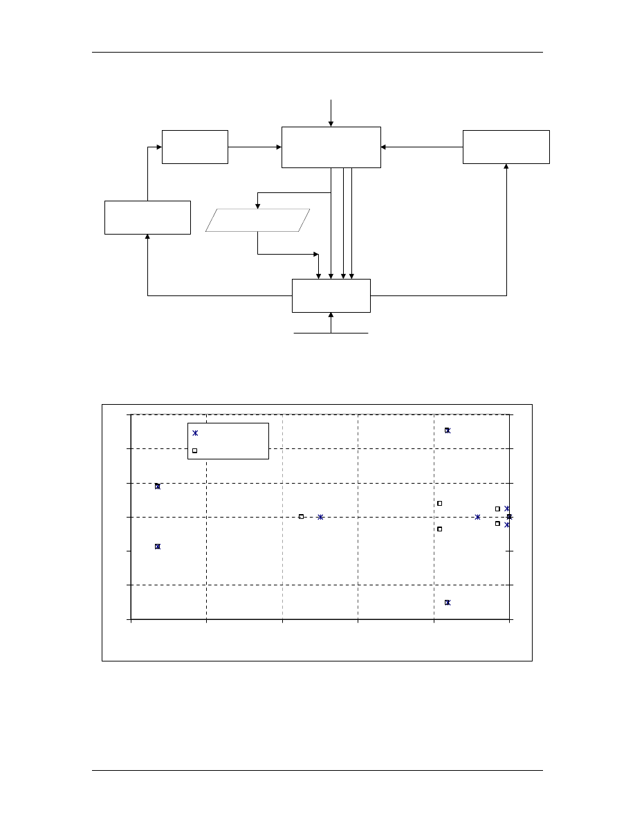
RDF Project CW02

Final Report

Global Energy Concepts, LLC

October 1, 2003

Turbine Plant

Power Electronics

Generator

Torque

State Space

Controller

Generator

RPM

Torque/Speed

Relationship

Torque

Command

Pitch

Torque

RPM Set

Point

Measurements of:

Blade Pitch

Tower Velocity

Blade Pitch

Controller and

Motor/Actuator

Wind

Disturbance

Pitch Rate Demand

to Position Demand

Integration

Nominal Pitch

Position

Figure 20. State space control flow diagram

-10

-8

-6

-4

-2

Real Part

, H

-3

-2

-1

Plant
Closed Loop

Figure 21. Plant and closed loop poles of the LTI model at 24 m/s

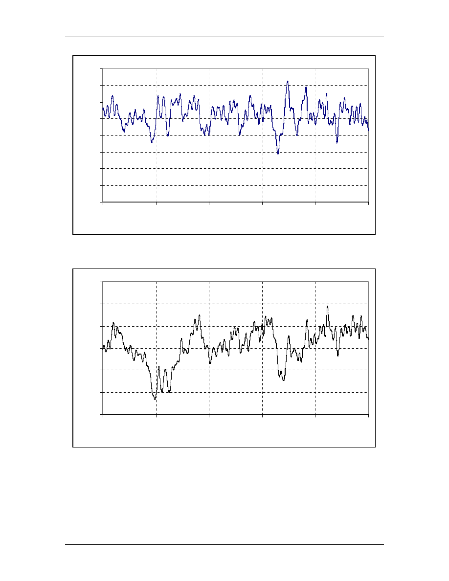
RDF Project CW02

Final Report

Global Energy Concepts, LLC

October 1, 2003

100

120

140

160

180

200

Time, seconds

Figure 22. Turbine rpm in 24 m/s turbulence

100

120

140

160

180

200

Time, seconds

itc

Figure 23. Collective blade pitch in 24 m/s turbulence

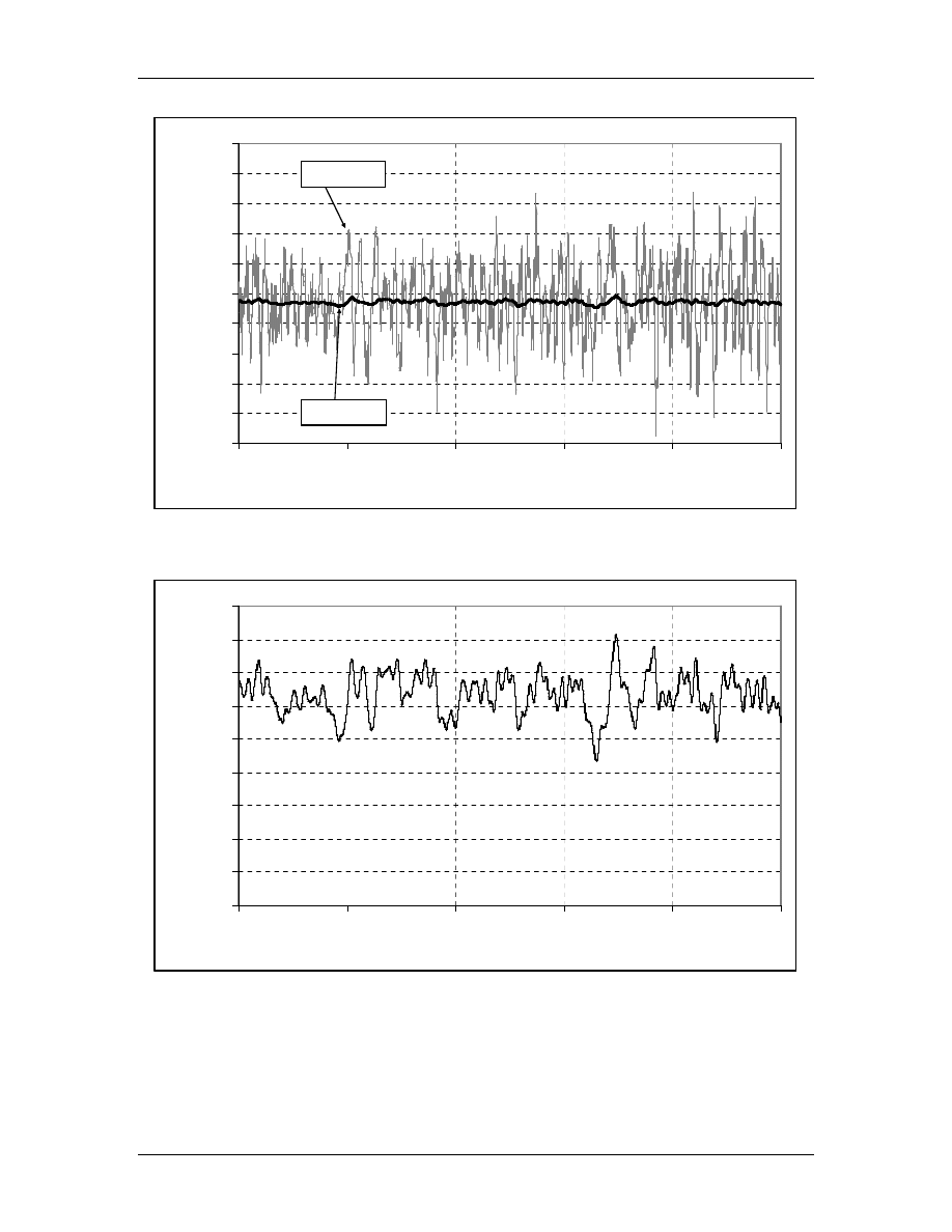
RDF Project CW02

Final Report

Global Energy Concepts, LLC

October 1, 2003

500

550

600

650

700

750

800

850

900

950

1000

100

120

140

160

180

200

Time, seconds

, k

Mainshaft

Generator

Figure 24. Drive train torques in 24 m/s turbulence

1000

1100

1200

1300

1400

1500

1600

1700

1800

1900

100

120

140

160

180

200

Time, seconds

l P

, k

Figure 25. Electrical power in 24 m/s turbulence

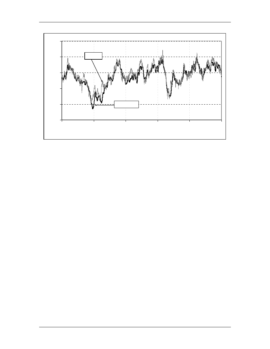
RDF Project CW02

Final Report

Global Energy Concepts, LLC

October 1, 2003

100

120

140

160

180

200

Time, seconds

, m

Actual

Estimated

Figure 26. Wind sped estimate versus actual hub height wind speed.

4 Conclusions

This project has successfully developed a tool that linearizes ADAMS models of wind

turbines. These linearizations can be used for modal analysis and control design. In

particular, the linearized models accurately contain the effects of aerodynamic and

rotational effects.

The ADAMS modeling environment is used fairly widely by wind turbine design and

research engineers. It is particularly useful because of its broad flexibility and capability

of modeling a wide range of configurations. With this linearization tool, and the

powerful flexibility of the ADAMS modeling environment, control designs can be

analyzed that encompass significant real world effects, including filters, digital controls

with time lag, and actuator and sensor dynamics. Configuration changes to plant model,

measurements, and control can be implemented fairly rapidly.

This tool will allow the further development and refinement of wind turbine controls.

Future work in this area could include studies that analyze the impact of sensor response

and placement, aerodynamic tailoring for control, and a wide variety of control methods.

RDF Project CW02

Final Report

Global Energy Concepts, LLC

October 1, 2003

5 References

Bossanyi, E., Developments in Closed Loop Controller Design for Wind Turbines,

Proceedings of the ASME Wind Energy Symposium, Reno, January 2000.

Bir, G., and Robinson, M., Code Development for Control Design Applications,

Proceedings of the ASME Wind Energy Symposium, Reno, January 1999.

Hodges, D., and Patil, M., Multi Flexible Body Analysis for Application to Wind

Turbine Control Design, Proceedings of the ASME Wind Energy Symposium, Reno,

January 2000.

Malcolm, David J., et. al., The Use of ADAMS to Model the AWT-26 Prototype,

Proceedings of the ASME Wind Energy Symposium, New Orleans, January 1994.

Malcolm, D.J. and McCoy, T.J., Results from the Advanced Research Turbine

Project, Proceedings of the ASME Wind Energy Symposium, Reno, January 2000.

Elliot, A. S., and Wright, A. D., ADAMS/WT: An Industry-Specific Interactive

Modeling Interface for Wind Turbine Analysis. Proceedings of the ASME Wind

Energy Symposium, New Orleans, 1994.

Elliot, Andrew S., ADAMS/WT Advanced Development – Version 1.4 and Beyond,

Proceedings of the American Wind Energy Conference, June 1996.

Global Energy Concepts, Advanced Methods for Development of Wind Turbine

Models for Control Design Phase I Status Report, Xcel Energy RDF Project CW02,

December 2002.

Malcolm, D.J., and Hansen, A.C., WindPACT Turbine Rotor Design Study,

NREL/SR-500-32495, National Renewable Energy Laboratory, August 2002.

10.

Hansen, A.C., User’s Guide for the YawDyn and Aerodyn for ADAMS, University of

Utah, January, 1996.

11.

Coleman, R.P. and Feingold, A.M., Theory of self-excited mechanical oscillations of

helicopter rotors with hinged blades, NACA Technical Report TR 1351, 1958.

12.

Dugundji, J., and Wendell, J.H., Review of analysis methods for rotating systems with

periodic coefficients, Proceedings of Wind Turbine Dynamics, NASA conference

publication 2185, DOE publication CONF-810226, Cleveland, Ohio, February 24-26,

1981.

13.

Malcolm, D.J., Modal Response of a 3 Bladed Wind Turbine, Journal of Solar Energy

Engineering, November 2002.

14.

Hansen, M. H., Improved Modal Dynamics of Wind Turbines to Avoid Stall Induced

Vibrations, Wind Energy, John Wiley and Sons, February 2003.

15.

Burl, Jeffery, B., Linear Optimal Control, Addison-Wesley, 1999.

RDF Project CW02

Final Report

Global Energy Concepts, LLC

A-1

October 1, 2003

Appendix A

Generalized Force Subroutine Code

! *****************************************************
!
SUBROUTINE GFOSUB( ID, ATIME, PAR, NPAR, DFLAG, IFLAG, ElemAeroF)
!
! Called by ADAMS to get element aerodynamic and rotational
! forces.for linearization
!
! *****************************************************

Parameter Nelem=15, Nws=12

IMPLICIT NONE

INTEGER ID, igrnd, ipitch, iblade, jelem, iwind, nctrl
INTEGER NPAR,n,nn, nnn, nw, i, j
INTEGER Mode, nstate, nvals, ivec(3), ns, nvec, ihub, nvar
INTEGER iaero, ibld1, ibld2, ibld3

DOUBLE PRECISION ATIME, WIND_INT, omega
DOUBLE PRECISION PAR( NPAR )
DOUBLE PRECISION ElemAeroF(6), bld_prop(4), temp(3)
DOUBLE PRECISION ELPITCH, ELEMVREL2G(3), ElemDrel2G(3,3)
DOUBLE PRECISION WIND_sym, WIND_sin, WIND_cos, Wind
DOUBLE PRECISION Bld_dsp(9), Bld_vel(9), Bld_rot(9), Bld_rvl(9)
Double Precision FD(9,9), FV(9,9), F(9), Fsave(3,3,Nelem)

REAL pi, PITNOW, DFN, DFT
REAL savp(7,3,Nelem) ! 7 states by 3 blades by Nelem blade parts
REAL Dvar(10) ! delta values of states
REAL aero_deriv(4,2,Nelem,Nws)
REAL bld_mass

LOGICAL DFLAG, errflg, IFLAG, FIRST

SAVE aero_deriv, savp, nw, first, omega, FD, FV, Fsave

! aero derivatives for Normal and Tangential Force vs blade pitch
! and normal and tangential velocity
! all w.r.t. the plane of rotation approximated by the hub coordinates
! break out normal velocity into body motion and wind as induction
! factor is applied differently

! Aero_deriv(2 forces (Fn and Ft), 4 variables (pitch, wind, Vnb, Vt),
! Nelem blade elements, Nws Wind speeds)

! Convert passed parameters to meaningful terms.

! USER passes ( Blade#, Section#, Control variable ID, Marker ) or
! ( IBlade, JElem, Nctrl, IAERO )
! IBlade = Blade ID number (1 to NB)
! JElem = Blade element ID number (1 to NELM)
! NCTRL = switch for aero (0) to rotating effects (2)
!
! IAERO = Aero or CG Marker ID number

IBlade = IDNINT( PAR(1) )
JElem = IDNINT( PAR(2) )
NCTRL = IDNINT( PAR(3) )
IAERO = IDNINT( PAR(4) )

call getmod (Mode) ! get mode of ADAMS, 6 is static solution, 7 is linearization

RDF Project CW02

Final Report

Global Energy Concepts, LLC

A-2

October 1, 2003

if (iflag .and. iblade .eq. 1 .and. jelem .eq. 1) then
OPEN(UNIT = 42, FILE = 'aero_deriv.dat', STATUS = 'UNKNOWN')
do nnn = 1,Nws
do nn = 1,Nelem
read(42,*) (aero_deriv(n,1,nn,nnn), n = 1,4) &
,(aero_deriv(n,2,nn,nnn), n = 1,4)
enddo
enddo
close(42)
first = .true.
pi = 4.0*atan(1.0)

! Build matrices for force computations

FD = 0.0
FV = 0.0

FD(1,1) = (2./3.)
FD(2,2) = (5./3.)
FD(3,3) = (5./3.)
FD(4:6,4:6) = FD(1:3,1:3)
FD(7:9,7:9) = FD(1:3,1:3)

FD(1,4) = -(1./3.)
FD(2,5) = -(5./6.)
FD(3,6) = -(5./6.)
FD(2,6) = -(1./2.)*sqrt(3.0)
FD(3,5) = (1./2.)*sqrt(3.0)
FD(4:6,7:9) = FD(1:3,4:6)
FD(7:9,1:3) = FD(1:3,4:6)

FD(1,7) = -(1./3.)
FD(2,8) = -(5./6.)
FD(3,9) = -(5./6.)
FD(2,9) = (1./2.)*sqrt(3.0)
FD(3,8) = -(1./2.)*sqrt(3.0)
FD(4:6,1:3) = FD(1:3,7:9)
FD(7:9,4:6) = FD(1:3,7:9)

FV(2,3) = 2.0
FV(3,2) = -2.0
FV(4:6,4:6) = FV(1:3,1:3)
FV(7:9,7:9) = FV(1:3,1:3)

FV(1,4) = -(2./3.)*sqrt(3.0)
FV(2,5) = (1./3.)*sqrt(3.0)
FV(3,6) = (1./3.)*sqrt(3.0)
FV(2,6) = -1.0
FV(3,5) = 1.0
FV(4:6,7:9) = FV(1:3,4:6)
FV(7:9,1:3) = FV(1:3,4:6)

FV(1,7) = (2./3.)*sqrt(3.0)
FV(2,8) = -(1./3.)*sqrt(3.0)
FV(3,9) = -(1./3.)*sqrt(3.0)
FV(2,9) = -1.0
FV(3,8) = 1.0
FV(4:6,1:3) = FV(1:3,7:9)
FV(7:9,4:6) = FV(1:3,7:9)

endif

if (first) then
! get the array index to the wind speed for use with aero_deriv
CALL INFFNC ( 'VARVAL', 9001, 1, WIND_INT, ERRFLG )

nw = idnint(wind_int)

! get the rotor rotation rate
CALL INFFNC ( 'VARVAL', 9002, 1, omega, ERRFLG )

first = .false.

endif

RDF Project CW02

Final Report

Global Energy Concepts, LLC

A-3

October 1, 2003

if (nctrl .eq. 2) then ! forces due to rotation

if (.not. iflag) then
call gtaray (iaero-10, bld_prop, nvals, errflg)
bld_mass = bld_prop(1) ! mass of current blade element
endif

! translational displacements and velocities for all 3 blades
! in global/ground coordinates

if (iblade .eq. 1) then
ibld1 = iaero
ibld2 = iaero + 10000
ibld3 = iaero + 20000
elseif( iblade .eq. 2) then
ibld1 = iaero - 10000
ibld2 = iaero
ibld3 = iaero + 10000
else
ibld1 = iaero - 20000
ibld2 = iaero - 10000
ibld3 = iaero
endif

IVEC(1) = ibld1
IVEC(2) = 4100+jelem
IVEC(3) = 10
NVEC = 3
CALL sysary('TDISP',IVEC, NVEC, Bld_dsp(1), NVALS, ERRFLG)
IVEC(2) = 4115 + jelem
CALL sysary('TVEL', IVEC, NVEC, Bld_vel(1), NVALS, ERRFLG)

IVEC(1) = ibld2
IVEC(2) = 4200 + jelem
IVEC(3) = 10
CALL sysary('TDISP',IVEC, NVEC, Bld_dsp(4), NVALS, ERRFLG)
IVEC(2) = 4215 + jelem
CALL sysary('TVEL', IVEC, NVEC, Bld_vel(4), NVALS, ERRFLG)

IVEC(1) = ibld3
IVEC(2) = 4300 + jelem
IVEC(3) = 10
CALL sysary('TDISP',IVEC, NVEC, Bld_dsp(7), NVALS, ERRFLG)
IVEC(2) = 4315 + jelem
CALL sysary('TVEL', IVEC, NVEC, Bld_vel(7), NVALS, ERRFLG)

F = omega*(omega*matmul(FD,Bld_dsp) + matmul(FV,Bld_vel))

! put forces into array for return to ADAMS, also convert to kN

ElemaeroF(1) = 0.001*bld_mass*F(1+(iblade-1)*3)
ElemaeroF(2) = 0.001*bld_mass*F(2+(iblade-1)*3)
ElemaeroF(3) = 0.001*bld_mass*F(3+(iblade-1)*3)
ElemaeroF(4) = 0.0
ElemaeroF(5) = 0.0
ElemaeroF(6) = 0.0

! suppress forces associated with perturbations in static mode
if (mode .eq. 6 .and. dflag) then
ElemaeroF(1) = Fsave(1,iblade,jelem)
ElemaeroF(2) = Fsave(2,iblade,jelem)
ElemaeroF(3) = Fsave(3,iblade,jelem)
else
Fsave(1,iblade,jelem) = ElemaeroF(1)
Fsave(2,iblade,jelem) = ElemaeroF(2)
Fsave(3,iblade,jelem) = ElemaeroF(3)
endif

RDF Project CW02

Final Report

Global Energy Concepts, LLC

A-4

October 1, 2003

Else ! for nctrl = 0: aero calcs

IGRND = 10
IHUB = 4010
IPITCH = 4191

! blade element total rotation, incl rigid body pitch and elastic twist

IVEC(1) = IAERO
IVEC(2) = IPITCH + 100 * ( IBLADE -1 ) ! Hub Ref Marker on hub side of pitch bearing
NVEC = 2
CALL SYSFNC ( 'AX', IVEC, NVEC, ELPITCH, ERRFLG )
Pitnow = SNGL ( ELPITCH )

! blade element translational velocity at aero marker
! realative to ground, but in blade coordinates

IVEC(1) = IAERO
IVEC(2) = IGRND
IVEC(3) = IHUB + Iblade
NVEC = 3
CALL sysary('TVEL', IVEC, NVEC, ElemVrel2G, NVALS, ERRFLG)

! blade element translational displacement for all blades
do n = 1,3
IVEC(1) = IAERO + 10000*(n - iblade)
IVEC(2) = IGRND
IVEC(3) = IHUB + n
NVEC = 3
CALL sysary('TDISP', IVEC, NVEC, ElemDrel2G(:,n), NVALS, ERRFLG)
enddo

! get the wind perturbations based on variables used in pinput list
iwind = 9120
CALL SYSFNC ( 'VARVAL', iwind, 1, WIND_sym, ERRFLG )
iwind = 9220
CALL SYSFNC ( 'VARVAL', iwind, 1, WIND_sin, ERRFLG )
iwind = 9320
CALL SYSFNC ( 'VARVAL', iwind, 1, WIND_cos, ERRFLG )

! Note that choice of element # in denom below is where Coleman wind field is defined
! e.g. 10 in denom implies 2/3rds out blade for 15 element blade

if (iblade .eq. 1) wind = wind_sym + wind_cos*float(jelem)/10.
if (iblade .eq. 2) wind = wind_sym + (0.866*wind_sin - 0.5*wind_cos)*float(jelem)/10.
if (iblade .eq. 3) wind = wind_sym + (-0.866*wind_sin - 0.5*wind_cos)*float(jelem)/10.

if (dflag .and. mode .eq. 7) then

DFN = 0.0
DFT = 0.0

Dvar(1) = pitnow - savp(7,iblade,jelem)
Dvar(2) = Wind
Dvar(3) = elemVrel2g(1) - savp(1,iblade,jelem)
Dvar(4) = elemVrel2g(2) - savp(2,iblade,jelem)
Dvar(5) = elemDrel2g(1,1) - savp(4,1,jelem)
Dvar(6) = elemDrel2g(2,1) - savp(5,1,jelem)
Dvar(7) = elemDrel2g(1,2) - savp(4,2,jelem)
Dvar(8) = elemDrel2g(2,2) - savp(5,2,jelem)
Dvar(9) = elemDrel2g(1,3) - savp(4,3,jelem)
Dvar(10) = elemDrel2g(2,3) - savp(5,3,jelem)

do nvar = 1,4
DFN = DFN + Dvar(nvar)*aero_deriv(nvar,1,jelem,nw)
DFT = DFT + Dvar(nvar)*aero_deriv(nvar,2,jelem,nw)
enddo

! aerodynamic forces with coupling effects as appropriate for blade #

RDF Project CW02

Final Report

Global Energy Concepts, LLC

A-5

October 1, 2003

if (iblade .eq. 1) then

DFN = DFN - (1./3.)*sqrt(3.)*omega* &
(-Dvar(7)*aero_deriv(3,1,jelem,nw) &
-Dvar(8)*aero_deriv(4,1,jelem,nw) &
+Dvar(9)*aero_deriv(3,1,jelem,nw) &
+Dvar(10)*aero_deriv(4,1,jelem,nw))
DFT = DFT - (1./3.)*sqrt(3.)*omega* &
(-Dvar(7)*aero_deriv(3,2,jelem,nw) &
-Dvar(8)*aero_deriv(4,2,jelem,nw) &
+Dvar(9)*aero_deriv(3,2,jelem,nw) &
+Dvar(10)*aero_deriv(4,2,jelem,nw))

elseif (iblade .eq. 2) then

DFN = DFN - (1./3.)*sqrt(3.)*omega* &
(+Dvar(5)*aero_deriv(3,1,jelem,nw) &
+Dvar(6)*aero_deriv(4,1,jelem,nw) &
-Dvar(9)*aero_deriv(3,1,jelem,nw) &
-Dvar(10)*aero_deriv(4,1,jelem,nw))
DFT = DFT - (1./3.)*sqrt(3.)*omega* &
(+Dvar(5)*aero_deriv(3,2,jelem,nw) &
+Dvar(6)*aero_deriv(4,2,jelem,nw) &
-Dvar(9)*aero_deriv(3,2,jelem,nw) &
-Dvar(10)*aero_deriv(4,2,jelem,nw))

elseif (iblade .eq. 3) then

DFN = DFN - (1./3.)*sqrt(3.)*omega* &
(-Dvar(5)*aero_deriv(3,1,jelem,nw) &
-Dvar(6)*aero_deriv(4,1,jelem,nw) &
+Dvar(7)*aero_deriv(3,1,jelem,nw) &
+Dvar(8)*aero_deriv(4,1,jelem,nw))
DFT = DFT - (1./3.)*sqrt(3.)*omega* &
(-Dvar(5)*aero_deriv(3,2,jelem,nw) &
-Dvar(6)*aero_deriv(4,2,jelem,nw) &
+Dvar(7)*aero_deriv(3,2,jelem,nw) &
+Dvar(8)*aero_deriv(4,2,jelem,nw))
endif

ElemAeroF(1) = DFN
ElemAeroF(2) = DFT
ElemAeroF(3) = 0.0D0
ElemAeroF(4) = 0.0D0
ElemAeroF(5) = 0.0D0
ElemAeroF(6) = 0.0D0

else
ElemAeroF(1) = 0.0D0
ElemAeroF(2) = 0.0D0
ElemAeroF(3) = 0.0D0
ElemAeroF(4) = 0.0D0
ElemAeroF(5) = 0.0D0
ElemAeroF(6) = 0.0D0

savp(1,iblade,jelem) = elemVrel2g(1)
savp(2,iblade,jelem) = elemVrel2g(2)
savp(3,iblade,jelem) = elemVrel2g(3)
savp(7,iblade,jelem) = pitnow

do n = 1,3 ! loop on 3 blades
savp(4,n,jelem) = elemDrel2g(1,n)
savp(5,n,jelem) = elemDrel2g(2,n)
savp(6,n,jelem) = elemDrel2g(3,n)
enddo

endif ! dflag loop

endif ! nctrl loop

RETURN

RDF Project CW02

Final Report

Global Energy Concepts, LLC

B-1

October1, 2003

Appendix B

ADAMS Model Elements

The following describes the elements of the ADAMS model required for implementation

of the procedures in this report via the subroutine of Appendix A.

Aerodynamic Derivatives
The subroutine reads in a 4x2x15x12 matrix that is stored in a file in an 8 x Nelem*Nws

matrix as follows:

∂

)

(

)

(

)

(

)

(

)

(

)

(

)

(

)

(

)

(

)

(

)

(

)

(

)

(

)

(

)

(

)

(

where x and y are in global coordinates, N = the number of blade elements (iterated first),

and M = the number of wind speed operating points.

Markers
The subroutine requires the following markers:

Marker #s

Part #s

Purpose

Location & Orientation

i1111 to

i2511

i = 1,3

i1100 to

i2500

i = 1,3

Blade element aerodynamic force

markers

At blade element center of

aerodynamic pressure, x

axis out blade

4i91 i=1,3

4i00 i=1,3

Reference markers on hub for pitch

measurement

On hub with x axes out

respective blades

401i i=1,3

4000

Define coordinate system for

measurement of blade element

velocities and displacements. Also

coordinate system for application of

blade aero forces.

On hub in standard blade

coordinate system per

blade

i1110 to

i2510

i = 1,3

i1100 to

i2500

i = 1,3

Blade element markers at center of

gravity

Not actually CM marker, but

same location with standard

blade coordinate orientation

4i01 to 4i15

ground

For displacement perturbation

measurement in rotational force

calculation

At hub center in blade

coordinate systems

4i16 to 4i30

ground

For velocity perturbation

measurement in rotational force

calculation

Superimposed on blade cg

in blade coordinate systems

RDF Project CW02

Final Report

Global Energy Concepts, LLC

B-2

October1, 2003

Variables
The subroutine requires the following variables:

Variable

Purpose

9001

Wind speed index for aero_deriv

matrix

9002

Rotor rotation rate in rad/sec

9003

Operating point pitch angle in rad

9120

Coleman symmetric wind disturbance

9220

Coleman sine wind disturbance

9320

Coleman cosine wind disturbance

Array i1100

to i2500

Contains blade element mass

Typically, the model is set up with the following input and output variables for the linear

model.

Variable

Description

Purpose

11000

Blade collective pitch demand

Control Input

21000

Blade sine pitch demand

Control Input

31000

Blade cosine pitch demand

Control Input

3000

Generator torque demand

Control Input

9120

Mean wind

Disturbance Input

9220

Sine wind (horizontal shear)

Disturbance Input

9320

Cosine wind (vertical shear)

Disturbance Input

3001

RPM

Measurement

3010

Power

Measurement

2007

Tower fore-aft velocity

Measurement

10001

Blade root flapwise collective moment Measurement

20001

Blade root flapwise sine moment

Measurement

30001

Blade root flapwise cosine moment

Measurement

RDF Project CW02

Final Report

Global Energy Concepts, LLC

B-3

October1, 2003

Parameters:
The following parameters are defined in the model.

Variable

Purpose

101

Blade pitching inertia, J, in kg·m

for

pitch actuator gain calculation

102

Blade pitch actuator time constant,

tau, in seconds for pitch actuator gain

calculation

113

Blade pitch actuator integral gain, K1

114

Blade pitch actuator proportional gain,

115

Blade pitch actuator kroportional gain,

116

Blade pitch actuator derivative gain,

117

Blade pitch actuator derivative gain,

Wyszukiwarka

Podobne podstrony:
Development of wind turbine control algorithms for industrial use
Development Of Wind Power Control System For Six Phase Permanent Magnet Synchronous Generators
Development of BBM turbine
[2006] Application of Magnetic Energy Recovery Switch (MERS) to Improve Output Power of Wind Turbine
[US 2006] D517986 Wind turbine and rotor blade of a wind turbine
Variable Speed Control Of Wind Turbines Using Nonlinear And Adaptive Algorithms
DESIGN AND DEVELOPMENT OF MICRO TURBINE
Stochastic Analysis Power Output of Wind Turbine
[US 2006] D517986 Wind turbine and rotor blade of a wind turbine
[2006] Application of Magnetic Energy Recovery Switch (MERS) to Improve Output Power of Wind Turbine
0 Renewable Energy Analysis Of A Wind Turbine Kelley 1997
CEI 61400 22 Wind turbine generator systems Required Design Documentation
CEI 61400 22 Wind turbine generator systems Required Design Documentation
Development Of A Single Phase Inverter For Small Wind Turbine

więcej podobnych podstron