Optical conductivity of graphene in the visible region of the spectrum

T. Stauber,

1

N. M. R. Peres,

1

and A. K. Geim

2

1

Centro de Física e Departamento de Física, Universidade do Minho, P-4710-057, Braga, Portugal

2

Manchester Centre for Mesoscience and Nanotechnology, University of Manchester, Manchester M12 9PL, United Kingdom

共Received 13 March 2008; published 26 August 2008

兲

We compute the optical conductivity of graphene beyond the usual Dirac-cone approximation, giving results

that are valid in the visible region of the conductivity spectrum. The effect of next-nearest-neighbor hopping is
also discussed. Using the full expression for the optical conductivity, the transmission and reflection coeffi-
cients are given. We find that even in the optical regime the corrections to the Dirac-cone approximation are
surprisingly small

共a few percent兲. Our results help in the interpretation of the experimental results reported by

Nair et al.

关Science 320, 1308 共2008兲兴.

DOI:

10.1103/PhysRevB.78.085432

PACS number

共s兲: 78.40.Ri, 81.05.Uw, 73.20.⫺r, 78.66.Tr

I. INTRODUCTION

Graphene, an atomically thin material made only of car-

bon atoms arranged in a hexagonal lattice, was isolated only
recently.

1

,

2

Several reviews on the physics of graphene are

already available in the literature.

3

–

6

At low energies, E

⬍1 eV, the electronic dispersion has

the form

⑀

共k兲= ⫾3tka/2, where t is the nearest-neighbor

hopping integral and a is the carbon-carbon distance. The
effective theory at these energy scales is that of a massless
Dirac Hamiltonian in

共2+1兲 dimensions. If the experimental

probes excite the system within this energy range, the Dirac
Hamiltonian is all there is for describing the physics of
graphene. On the other hand, for excitations out of this en-
ergy range, it is necessary to include corrections to the Dirac
Hamiltonian, which will modify the energy spectrum and
thus the density of states of the system. One immediate con-
sequence is that the energy dispersion is no longer a function
of the absolute value of the wave number k. In this paper, we
will calculate the optical conductivity of graphene including
the leading corrections to the Dirac-cone approximation.

One of the first calculations of the optical conductivity of

graphene using the Dirac Hamiltonian were done by Gusynin
and Sharapov.

7

This first study was subsequently revisited a

number of times

8

–

10

and summarized in Ref.

11

. However,

these authors did not include nonlinear effects in the calcu-
lation. Also the effect of disorder was done on a phenomeno-
logical level, by broadening the delta functions into Lorent-
zians characterized by a constant width

⌫. We note that in the

Dirac-cone approximation, the conductivity can also be ob-
tained from the polarization. The calculations for finite
chemical potential and arbitrary

兩q兩 and

␻

were done by

Wunsch et al.

12

and Hwang and Das Sarma.

13

The calculation of the optical conductivity of graphene, in

the Dirac Hamiltonian limit, including the effect of disorder
in a self-consistent way was done by Peres et al.,

14

and re-

cently also corrections due to electron-electron interaction
were discussed.

15

,

16

The calculation for the graphene bilayer

with disorder was done by Koshino and Ando

17

and by Nils-

son et al.

18

The optical conductivity of a clean bilayer was

first computed by Abergel and Fal’ko

19

and recently gener-

alized to the biased

20

–

22

bilayer case by Nicol and Carbotte.

23

Within the Boltzmann approach, the optical conductivity

of graphene was considered in Refs.

24

and

25

where the

effect of phonons and the effect of midgap states were in-
cluded. This approach, however, does not include transitions
between the valence and the conduction band and is, there-
fore, restricted to finite doping. The voltage and the tem-
perature dependence of the conductivity of graphene were
considered by Vasko and Ryzhii

26

using the Boltzmann ap-

proach. The same authors have recently computed the pho-
toconductivity of graphene, including the effect of acoustic
phonons.

27

The effect of temperature on the optical conductivity

of clean graphene was considered by Falkovsky and
Varlamov.

28

The far-infrared properties of clean graphene

were studied in Ref.

29

and

30

. Also this study was restricted

to the Dirac-spectrum approximation.

It is interesting to note that the conductivity of clean

graphene, at half filling and in the limit of zero temperature,
is given by the universal value of

␲

e

2

/共2h兲.

31

,

32

On the other

hand, if the temperature is kept finite the conductivity goes to
zero at zero frequency, but the effect of optical phonons does
not change the value of the conductivity of clean graphene.

33

This behavior should be compared with the calculation of the
dc conductivity of disordered graphene which, for zero
chemical potential, presents the value of 4e

2

/共

␲

h

兲.

14

,

31

,

34

,

35

From the experimental point of view, the work of Kuz-

menko et al.

36

studied the optical conductivity of graphite

in the energy range of

关0,1兴 eV and showed that its beha-

vior is close to that predicted for clean graphene in that
energy range. An explanation of this odd fact was attempted
within the Slonczewski-McClure-Weiss model. The complex
dielectric constant of graphite was studied by Pedersen

37

for all energy ranges. The infrared spectroscopy of Landau
levels in graphene was studied by Jiang et al.

38

and Deacon

et al.,

39

confirming the magnetic field dependence of the

energy levels and deducing a band velocity for graphene
of 1.1

⫻10

6

m

/s. Recently, the infrared conductivity of a

single graphene sheet was obtained.

40

,

41

Recent studies of graphene multilayers grown on SiC

from terahertz to visible optics showed a rather complex
behavior

42

with values of optical conductivity close to those

predicted for graphene at infrared frequencies as well as to
those measured in graphite.

36

This experiment

42

especially

indicates the need for a graphene theory valid all the way to
optical frequencies. The absorption spectrum of multilayer
graphene in high magnetic fields was recently discussed in

PHYSICAL REVIEW B 78, 085432

共2008兲

1098-0121/2008/78

共8兲/085432共8兲

©2008 The American Physical Society

085432-1

Ref.

43

, including corrections to the Dirac-cone approxima-

tion.

In this paper we address the question of how the conduc-

tivity of clean graphene changes when one departs from the
linear spectrum approach. This is an important question for
experiments done in the visible region of the spectrum.

44

The

paper is organized as follows: in Sec. II we introduce our
model and derive the current operator; in Sec. III we discuss
the optical conductivity of graphene by taking into account
its full density of states; in Sec. IV we discuss the effect on
the optical conductivity of a next-nearest-neighbor hopping
term; in Sec. V we analyze the scattering of light by a
graphene plane located at the interface of two different di-
electrics and give the transmissivity and reflectivity curves in
the visible region of the spectrum; and finally in Sec. VI we
give our conclusions.

II. HAMILTONIAN AND THE CURRENT OPERATORS

The Hamiltonian, in tight-binding form, for electrons in

graphene is written as

H = − t

兺

R,

␴

兺

␦

=

␦

1

−

␦

3

关a

␴

†

共R兲b

␴

共R +

␦

兲 + H.c.兴

−

t

⬘

2

兺

R,

␴

兺

␦

=

␦

4

−

␦

9

关a

␴

†

共R兲a

␴

共R +

␦

兲 + H.c.兴

−

t

⬘

2

兺

R,

␴

兺

␦

=

␦

4

−

␦

9

关b

␴

†

共R兲b

␴

共R +

␦

兲 + H.c.兴,

共1兲

where the operator a

␴

†

共R兲 creates an electron in the carbon

atoms of sublattice A, whereas b

␴

†

共R兲 does the same in sub-

lattice B; t is the hopping parameter connecting first-nearest
neighbors, with a value of the order of 3 eV; and t

⬘

is the

hopping parameter for second-nearest neighbors, with a
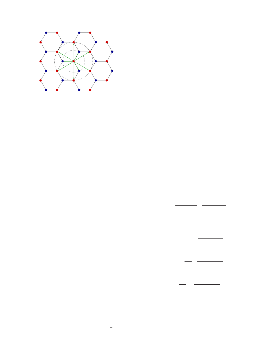
value of the order of 0.1t. The vectors

␦

i

are represented in

Fig.

1

and have the form

␦

1

=

a

2

共1,

冑

3

兲,

␦

2

=

a

2

共1,−

冑

3

兲,

␦

3

= − a

共1,0兲,

␦

4

= a

共0,

冑

3

兲,

␦

5

= −

␦

4

,

␦

6

=

3a

2

冉

1,

1

冑

3

冊

,

␦

7

= −

␦

6

,

␦

8

=

3a

2

冉

1,−

1

冑

3

冊

,

␦

9

= −

␦

8

.

共2兲

In order to obtain the current operator we modify the hop-
ping parameters as

t

→ te

i

关e/ប兴A共t兲·

␦

,

共3兲

and the same for t

⬘

. Expanding the exponential up to second

order in the vector potential A

共t兲 and assuming that the elec-

tric field is oriented along the x direction, the current opera-
tor is obtained from

j

x

= −

⳵

H

⳵

A

x

共t兲

,

共4兲

leading to j

x

= j

x

P

+ A

x

共t兲j

x

D

. The operator j

x

P

reads

j

x

P

=

tie

ប

兺

R,

␴

兺

␦

=

␦

1

−

␦

3

关

␦

x

a

␴

†

共R兲b

␴

共R +

␦

兲 − H.c.兴

+

t

⬘

ie

2

ប

兺

R,

␴

兺

␦

=

␦

4

−

␦

9

关

␦

x

a

␴

†

共R兲a

␴

共R +

␦

兲 − H.c.兴

+

t

⬘

ie

2

ប

兺

R,

␴

兺

␦

=

␦

4

−

␦

9

关

␦

x

b

␴

†

共R兲b

␴

共R +

␦

兲 − H.c.兴.

共5兲

The operator j

x

D

can be found from the linear term in A

x

共t兲

expansion of the Hamiltonian.

III. OPTICAL CONDUCTIVITY

A. Kubo formula

The Kubo formula for the conductivity is given by

␴

xx

共

␻

兲 =

具j

x

D

典

iA

s

共

␻

+ i0

+

兲

+

⌳

xx

共

␻

+ i0

+

兲

i

បA

s

共

␻

+ i0

+

兲

,

共6兲

with A

s

= N

c

A

c

, the area of the sample and A

c

= 3

冑

3a

2

/2 共a is

the carbon-carbon distance

兲, the area of the unit cell; from

which it follows that

R

␴

xx

共

␻

兲 = D

␦

共

␻

兲 +

I

⌳

xx

共

␻

+ i0

+

兲

ប

␻

A

s

,

共7兲

and

I

␴

xx

共

␻

兲 = −

具j

x

D

典

A

s

␻

−

R

⌳

xx

共

␻

+ i0

+

兲

ប

␻

A

s

,

共8兲

where D is the charge stiffness, which reads

D = −

␲

具j

x

D

典

A

s

−

␲

R

⌳

xx

共

␻

+ i0

+

兲

បA

s

.

共9兲

The function

⌳

xx

共

␻

+ i0

+

兲 is obtained from the Matsubara

current-current correlation function defined as

⌳

xx

共i

␻

n

兲 =

冕

0

ប

␤

d

␶

e

i

␻

n

␶

具T

␶

j

x

P

共

␶

兲j

x

P

共0兲典.

共10兲

In what follows we start by neglecting the contribution of t

⬘

to the current operator. Its effect is analyzed later and shown

a

A

B

δ

4

δ

5

δ

7

δ

8

δ

9

δ

3

δ

1

δ

2

δ

6

FIG. 1.

共Color online兲 Representation of the vectors

␦

i

, with i

= 1 – 9. The carbon-carbon distance a and the A and B atoms are
also depicted.

STAUBER, PERES, AND GEIM

PHYSICAL REVIEW B 78, 085432

共2008兲

085432-2

to be negligible. The function I

⌳

xx

共

␻

+ i0

+

兲 is given by

I

⌳

xx

共

␻

+ i0

+

兲 =

t

2

e

2

a

2

8

ប

2

兺

k

f

关

␾

共k兲兴关n

F

共− t兩

␾

共k兲兩 −

␮

兲

− n

F

共t兩

␾

共k兲兩 −

␮

兲兴关

␲

␦

共

␻

− 2t

兩

␾

共k兲兩/ប兲

−

␲

␦

共

␻

+ 2t

兩

␾

共k兲兩/ប兲兴,

共11兲

where n

F

共x兲 is the usual Fermi distribution,

␮

is the chemical

potential, and the function R

⌳

xx

共

␻

+ i0

+

兲 is given by

R

⌳

xx

共

␻

+ i0

+

兲 = −

t

2

e

2

a

2

8

ប

2

P

兺

k

f

关

␾

共k兲兴关n

F

共− t兩

␾

共k兲兩 −

␮

兲

− n

F

共t兩

␾

共k兲兩 −

␮

兲兴

4t

兩

␾

共k兲兩

␻

2

−

共2兩

␾

共k兲兩兲

2

,

共12兲

with

f

关

␾

共k兲兴 = 18 − 4兩

␾

共k兲兩

2

+ 18

关R

␾

共k兲兴

2

−

关I

␾

共k兲兴

2

兩

␾

共k兲兩

2

,

共13兲

and

P denotes the principal part of the integral. The

graphene energy bands are given by

⑀

共k兲= ⫾t兩

␾

共k兲兩, with

␾

共k兲 defined as

␾

共k兲 = 1 + e

k·

共

␦

1

−

␦

3

兲

+ e

k·

共

␦

2

−

␦

3

兲

.

共14兲

B. Real part of the conductivity

The expression for Eq.

共

11

兲 can almost be written in terms

of the energy dispersion

⑀

共k兲 except for the term

关R

␾

共k兲兴

2

−

关I

␾

共k兲兴

2

兩

␾

共k兲兩

2

.

共15兲

In order to proceed analytically, and for the time being

共see

Sec. III C

兲, we approximate this term by its value calculated

in the Dirac-cone approximation

共see Appendix A兲

1

N

c

兺

k

关R

␾

共k兲兴

2

−

关I

␾

共k兲兴

2

兩

␾

共k兲兩

2

g

共兩

␾

共k兲兩兲 ⯝ 0,

共16兲

where g

共兩

␾

共k兲兩兲 is some given function depending only on

the modulus of

␾

共k兲. With this approximation, we have

f

关

␾

共k兲兴 ⯝ 18 − 4兩

␾

共k兲兩

2

.

共17兲

Introducing the density of states per spin per unit cell

␳

共E兲

defined as

␳

共E兲 =

1

N

c

兺

k

␦

共E − t兩

␾

k

兩兲,

共18兲

the expression for the real part of the conductivity reads

R

␴

xx

共

␻

兲 =

␴

0

␲

t

2

a

2

8A

c

ប

␻

␳

共ប

␻

/2兲关18 − 共ប

␻

兲

2

/t

2

兴

⫻

冋

tanh

ប

␻

+ 2

␮

4k

B

T

+ tanh

ប

␻

− 2

␮

4k

B

T

册

.

共19兲

Equation

共

19

兲 is essentially exact in the visible range of the

spectrum; missing is only the contribution coming from Eq.

共

16

兲, whose contribution will later be shown to be negligible.

In the above equation,

␴

0

is

␴

0

=

␲

2

e

2

h

.

共20兲

The momentum integral in Eq.

共

18

兲 can be performed lead-

ing to

␳

共E兲 =

2E

t

2

␲

2

冦

1

冑

F

共E/t兲

K

冉

4E

/t

F

共E/t兲

冊

, 0

⬍ E ⬍ t,

1

冑

4E

/t

K

冉

F

共E/t兲

4E

/t

冊

,

t

⬍ E ⬍ 3t,

冧

共21兲

where F

共x兲 is given by

F

共x兲 = 共1 + x兲

2

−

共x

2

− 1

兲

2

4

,

共22兲

and K

共m兲 is defined as

K

共m兲 =

冕

0

1

dx

关共1 − x

2

兲共1 − mx

2

兲兴

−1

/2

.

共23兲

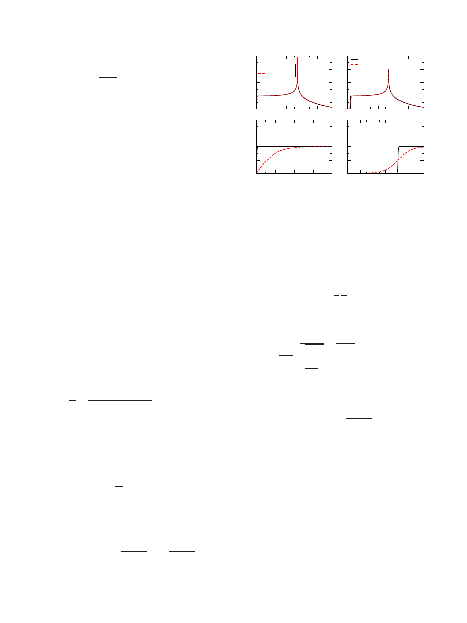
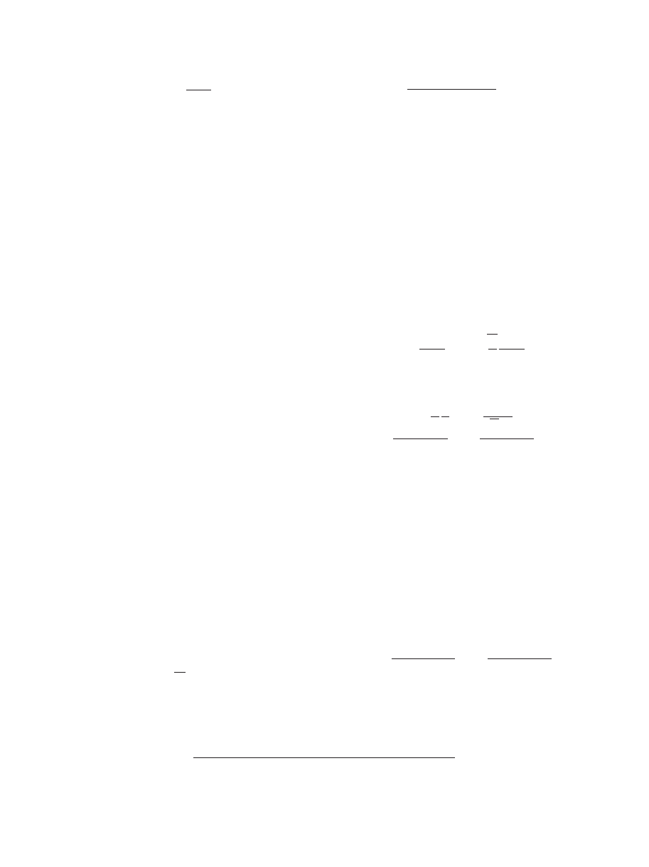
In Fig.

2

we give a plot of Eq.

共

19

兲 over a large energy

range

including

the

visible

part

of

the

spectrum

共E苸关1.0,3.1兴 eV兲.

It is useful to derive from Eq.

共

19

兲 an asymptotic expan-

sion for R

␴

xx

共

␻

兲. For that, we expand the density of states

around E = 0 and obtain

␳

共E兲 ⯝

2E

冑

3

␲

t

2

+

2E

3

3

冑

3

␲

t

4

+

10E

5

27

冑

3

␲

t

6

.

共24兲

Using Eq.

共

24

兲 in Eq. 共

19

兲 we obtain for the optical conduc-

tivity the approximate result

0

2

4

6

8

10

0

1

2

3

4

σ/σ

0

µ=0, T=10 K
µ=0, T=300 K

0

2

4

6

8

10

0

1

2

3

4

µ=0.2 eV, T= 10K
µ=0.2 eV, T= 300K

0

0.1

0.2

0.3

0.4

ω (eV)

0

0.5

1

1.5

2

σ/

σ

0

0

0.1

0.2

0.3

0.4

0.5

ω (eV)

0

0.5

1

1.5

2

FIG. 2.

共Color online兲 The optical conductivity as function of

frequency for two values of the chemical potential,

␮=0 and 0.2 eV,

and two temperatures, T = 10 and 300 K. The bottom panels are a
zoom in, close to zero frequency, which allow depicting the fre-
quency region where differences in the chemical potential and in
temperature are most important. We have used t = 2.7 eV.

OPTICAL CONDUCTIVITY OF GRAPHENE IN THE

…

PHYSICAL REVIEW B 78, 085432

共2008兲

085432-3

R

␴

xx

共

␻

兲 =

␴

0

冋

1

2

+

1

72

共ប

␻

兲

2

t

2

册

⫻

冉

tanh

ប

␻

+ 2

␮

4k

B

T

+ tanh

ប

␻

− 2

␮

4k

B

T

冊

.

共25兲

In the case of

␮

= 0 this expression is the same as in Kuz-

menko et al.

36

and in Falkovsky and Pershoguba

29

if in both

cases the

共ប

␻

/t兲

2

term is neglected.

C. Correction to R

␴

xx

(

␻) introduced by Eq. (

16

)

We now want to make the effect of the term given by Eq.

共

16

兲, which was neglected in Eq. 共

19

兲, quantitative. To that

end we expand the function

␾

共k兲 up to third order in mo-

mentum. The expansion is

␾

共k兲 ⯝

3a

2

共k

y

− ik

x

兲 +

1

2

冉

3a

2

冊

2

共k

x

2

+ k

y

2

/3 + 2ik

x

k

y

兲

+

1

6

冉

3a

2

冊

3

共ik

x

3

− k

y

3

/3 − 3k

x

2

k

y

+ ik

y

2

k

x

兲.

共26兲

The angular integral in Eq.

共

16

兲 leads to

冕

0

2

␲

d

␪

兵关R

␾

共k兲兴

2

−

关I

␾

共k兲兴

2

其 =

␲

24

冉

3ak

2

冊

4

,

共27兲

where we still assume

兩

␾

共k兲兩=3ak/2. Within this approxima-

tion the contribution to the conductivity coming from Eq.

共

16

兲 has the form

R

␴

xx

u

共

␻

兲 =

␴

0

1

4 ! 2

4

冉

ប

␻

t

冊

2

冉

tanh

ប

␻

+ 2

␮

4k

B

T

+ tanh

ប

␻

− 2

␮

4k

B

T

冊

.

共28兲

Due to the prefactor, this contribution has only a small effect
and shows that the current operator basically conserves the
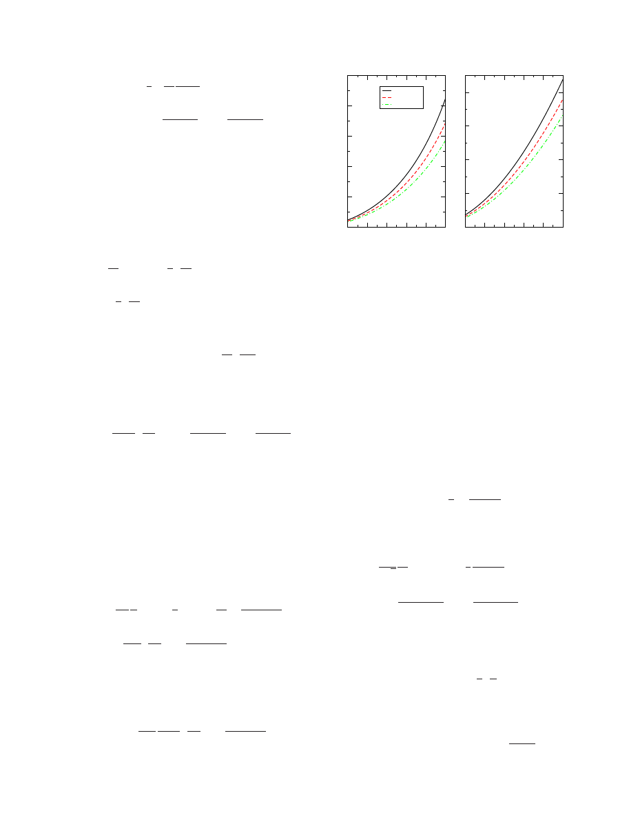
circular symmetry found close to the K points. In Fig.

3

we

present

␴

共

␻

兲/

␴

0

as a function of the frequency, considering

several values of t, in the optical range and also discuss the
numerical value of the term given in Eq.

共

28

兲.

D. Imaginary part of the conductivity

Neglecting the term proportional to Eq.

共

15

兲, the imagi-

nary part of the conductivity is given by

I

␴

xx

共

␻

兲 =

1

ប

␻

4

␲

␴

0

冉

␮

−

2

9

␮

3

/t

2

冊

−

␴

0

␲

log

兩ប

␻

+ 2

␮

兩

兩ប

␻

− 2

␮

兩

−

␴

0

36

␲

冉

ប

␻

t

冊

2

log

兩ប

␻

+ 2

␮

兩

兩ប

␻

− 2

␮

兩

,

共29兲

where we have included all the terms that diverge at

ប

␻

= 2

␮

and the contribution from the cubic term in frequency

in the density of states. The contribution of the last term of

f

关

␾

共k兲兴 in Eq. 共

13

兲 is given by

I

␴

xx

u

共

␻

兲 = −

␴

0

18

␲

1

4 ! 2

4

冉

ប

␻

t

冊

2

log

兩ប

␻

+ 2

␮

兩

兩ប

␻

− 2

␮

兩

.

共30兲

If we neglect the terms in

␮

3

and

␻

2

we obtain the same

expressions as those derived by Falkovsky and Pershoguba.

29

We note that these terms are also obtained from the polariz-
ability in the limit q

→0 since the Fermi velocity is not k

dependent.

12

E. Drude weight and the Hall coefficient

The Drude weight

共or charge stiffness兲 defined by Eq. 共

9

兲

can be computed in different limits. In the case

␮

= 0 we are

interested in its temperature dependence. For zero tempera-
ture the exact relation

兺

k

兩

␾

共k兲兩 =

1

8

兺

k

f

关

␾

共k兲兴

兩

␾

共k兲兩

共31兲

assures that D = 0 when

␮

= 0. In general, the Drude weight

has the following form:

D

共T,

␮

兲 = t

␴

0

4

␲

2

3

冑

3

1

N

c

兺

k

再

兩

␾

共k兲兩 −

1

8

f

关

␾

共k兲兴

兩

␾

共k兲兩

冎

⫻

冋

tanh

t

兩

␾

共k兲兩 +

␮

2k

B

T

+ tanh

t

兩

␾

共k兲兩 −

␮

2k

B

T

册

.

共32兲

In the case of finite

␮

, the temperature dependence of

D

共T,

␮

兲 is negligible. In the Dirac-cone approximation we

obtain

D

共0,

␮

兲 = 4

␲␴

0

␮

冋

1 −

1

9

冉

␮

t

冊

2

册

.

共33兲

On the other hand, at zero chemical potential, the tempera-
ture dependence of the charge stiffness is given by

D

共T,0兲 = 8

␲

ln 2

␴

0

k

B

T − 4

␲␨

共3兲

␴

0

共k

B

T

兲

3

t

2

,

共34兲

where

␨

共x兲 is the Riemann zeta function.

1

1.5

2

2.5

3

3.5

ω (eV)

1

1.02

1.04

1.06

1.08

1.1

σ/

σ

0

t=2.7 eV

t=2.9 eV

t=3.1 eV

1

1.5

2

2.5

3

3.5

ω (eV)

0

0.002

0.004

0.006

0.008

σ

u

/σ

0

FIG. 3.

共Color online兲 Left:

␴共␻兲/␴

0

as a function of the fre-

quency, including both Eq.

共

19

兲 and the correction to R

␴

xx

u

given by

Eq.

共

28

兲, for several values of t. Right: The correction to R

␴

xx

u

given by Eq.

共

28

兲 for several values of t. It is clear that the contri-

bution from this term has no bare effect on the results given by Eq.
共

19

兲. The calculations are for zero chemical potential and for room

temperature

关there is no visible effect on

␴共␻兲/␴

0

in the visible

range of the spectrum when compared to a zero-temperature
calculation

兴.

STAUBER, PERES, AND GEIM

PHYSICAL REVIEW B 78, 085432

共2008兲

085432-4

Zotos et al.

45

,

46

have shown a very general relation be-

tween the Drude weight and the Hall coefficient. This rela-
tion is

R

H

= −

1

eD

⳵

D

⳵

n

.

共35兲

Equation

共

35

兲 does not take into account the possibility of

valley degeneracy and therefore it has to be multiplied by 2
when we apply it to graphene. In the case of a finite chemical
potential, we have the following relations between the Fermi
wave vector k

F

and the chemical potential: n = k

F

2

/

␲

and

␮

= 2tak

F

/3. Applying Eq. 共

35

兲 to graphene we obtain

R

H

= −

2

e

n

−1

/2

/2 − 3a

2

冑

n

/8

冑

n − a

2

n

3

/2

/4

⯝ −

1

en

.

共36兲

IV. EFFECT OF t

⬘

ON THE CONDUCTIVITY

OF GRAPHENE

In this section we want to discuss the effect of t

⬘

on the

conductivity of graphene. One important question is what
value of t

⬘

is in graphene. Deacon et al.

39

proposed that the

dispersion for graphene, obtained from a tight-binding ap-
proach with nonorthogonal basis functions, is of the form

E =

⫾

t

兩

␾

共k兲兩

1

⫿ s

0

兩

␾

共k兲兩

共37兲

with

兩

␾

共k兲兩⯝

3
2

ka and with a, the carbon-carbon distance. On

the other hand the dispersion of graphene including t

⬘

has the

form

E =

⫾ t

3

2

ka − t

⬘

冋

9

4

共ka兲

2

− 3

册

.

共38兲

To relate t

⬘

and s

0

we expand Eq.

共

37

兲 as

E

⯝ ⫾ t兩

␾

共k兲兩共1 ⫾ s

0

兩

␾

共k兲兩兲 = ⫾ t

3

2

ka + s

0

t

9

4

共ka兲

2

,

共39兲

which leads to t

⬘

/t=−s

0

with s

0

= 0.13.

For computing the conductivity of graphene we need to

know the Green’s function with t

⬘

. These can be written in

matrix form as

G

0

共k,i

␻

n

兲 =

兺

␣=+,−

1

/2

i

␻

n

−

␣

t

兩

␾

共k兲兩/ប + 2t

⬘

关兩

␾

共k兲兩

2

− 3

兴/ប

⫻

冉

1

−

␣␾

共k兲/兩

␾

共k兲兩

−

␣␾

共k兲

ⴱ

/兩

␾

共k兲兩

1

冊

,

共40兲

where

G

0

共k,i

␻

n

兲 stands for

G

0

共k,i

␻

n

兲 =

冉

G

AA

共k,i

␻

n

兲 G

AB

共k,i

␻

n

兲

G

BA

共k,i

␻

n

兲 G

BB

共k,i

␻

n

兲

冊

.

共41兲

From Eq.

共

40

兲 we see that only the poles are modified with

the coherence factors having the same form as in the case
with t

⬘

= 0. The current operator j

x

P

= j

x,t

P

+ j

x,t

⬘

P

, as derived from

the tight-binding Hamiltonian is written in momentum space
as

j

x,t

P

=

tiea

2

ប

兺

␴

兺

k

兵关

␾

共k兲 − 3兴a

␴,k

†

b

␴,k

−

关

␾

ⴱ

共k兲 − 3兴b

␴,k

†

a

␴,k

其,

共42兲

and

j

x,t

⬘

P

=

3t

⬘

iea

2

ប

兺

␴

兺

k

关

␾

共k兲 −

␾

ⴱ

共k兲兴共a

␴,k

†

a

␴,k

+ b

␴,k

†

b

␴,k

兲.

共43兲

The operators j

x,t

P

and j

x,t

⬘

P

are the current operators associated

with the hopping amplitudes t and t

⬘

, respectively. The

current-current correlation function is now a sum of three
different terms: one where we have two j

x,t

P

operators, an-

other one where we have a j

x,t

P

and a j

x,t

⬘

P

, and a third one with

two j

x,t

⬘

P

. This last term vanishes exactly, since it would cor-

respond to the current-current correlation function of a trian-
gular lattice. Also the crossed term vanishes exactly, which
can be understood by performing a local gauge transforma-
tion to the fermionic operators of one sublattice only.
The first term leads to a contribution of the same form
as in Eq.

共

19

兲 but with the numerators of the two tanh

replaced by E

+

=

ប

␻

+ 2t

⬘

关共ប

␻

兲

2

/共4t

2

兲−3兴+2

␮

and E

−

=

ប

␻

− 2t

⬘

关共ប

␻

兲

2

/共4t

2

兲−3兴−2

␮

, respectively.

As a consequence of the effect of t

⬘

in the conductivity, a

graphene only enters in the band structure E

⫾

in the Fermi

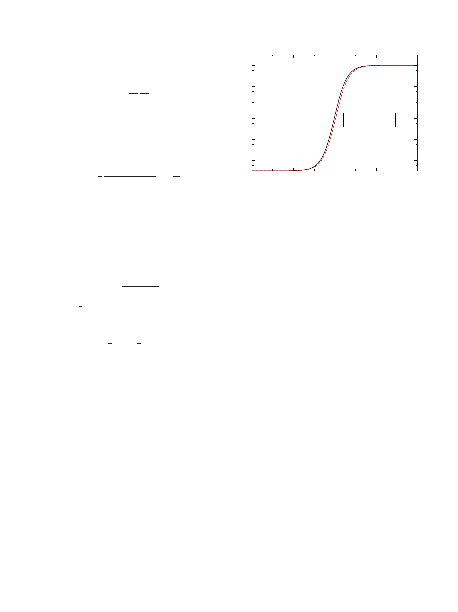
functions. In Fig.

4

we plot the real part of the optical con-

ductivity for two different values of

␮

: one with the Fermi

energy in the conduction band and the other with the Fermi
energy in the valence band. There is a small effect near twice
the absolute value of the chemical potential due to the break-
ing of particle-hole symmetry introduced by t

⬘

. For optical

frequencies, the effect of t

⬘

is negligible.

0.1

0.15

0.2

0.25

ω (eV)

0

0.1

0.2

0.3

0.4

0.5

0.6

0.7

0.8

0.9

1

1.1

σ/

σ

0

µ=0.1 eV, T=45 K
µ=-0.1 eV, T=45 K

FIG. 4.

共Color online兲 Real part of the conductivity for two

values of the chemical potential at the temperature of 45 K. The
parameters used are t = 3.1 eV and t

⬘

= −0.13t. Only the energy

range of

␻苸关0.1,0.3兴 eV is shown because only here the

chemical-potential difference has any noticeable effect.

OPTICAL CONDUCTIVITY OF GRAPHENE IN THE

…

PHYSICAL REVIEW B 78, 085432

共2008兲

085432-5

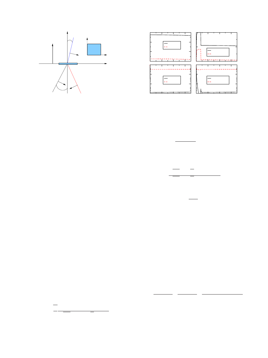
V. ELECTROMAGNETIC SCATTERING PROBLEM

Here we derive the reflectivity and the transmissivity of

light between two media, characterized by electrical permit-
tivities

⑀

i

⑀

0

with i = 1 , 2, separated by a graphene flake. The

scattering geometry is represented in Fig.

5

, i.e., we assume

the field to propagate in the direction k =

共k

x

, 0 , k

z

兲.

In the following, we assume the field to be given by E

=

共E

x

, 0 , E

z

兲 共p polarization兲. The case of s polarization is

addressed in Appendix B.

The electromagnetic boundary conditions then are

47

共D

2

− D

1

兲 · n =

␳

,

共44兲

n

⫻ 共E

2

− E

1

兲 = 0,

共45兲

where

␳

is the surface charge density, in our case the

graphene charge density. If we represent the intensity of the
incident, reflected, and transmitted electric field as E

i

, E

r

,

and E

t

, respectively, the boundary conditions can be written

as

共E

i

− E

r

兲cos

␪

1

= E

t

cos

␪

2

,

共46兲

−

⑀

2

⑀

0

E

t

sin

␪

2

+

⑀

1

⑀

0

共E

i

+ E

r

兲sin

␪

1

=

␳

,

共47兲

where

⑀

0

is the vacuum permittivity,

⑀

1

and

⑀

2

are the relative

permittivity of the two media, and

␪

1

and

␪

2

are the incident

and refracted angle, respectively. Now the continuity equa-
tion in momentum space reads

␳

共

␻

兲 = j

x

共

␻

兲k

x

/

␻

,

共48兲

and Ohm’s law is written as

j

x

共

␻

兲 =

␴

共

␻

兲E

x

=

␴

共

␻

兲E

t

cos

␪

2

.

共49兲

Combining Eqs.

共

46

兲–共

49

兲, we arrive at the following result,

valid for normal incidence, for the transmissivity T:

T =

冑

⑀

2

⑀

1

4

共

⑀

1

⑀

0

兲

2

兩共

冑

⑀

1

⑀

2

+

⑀

1

兲

⑀

0

+

冑

⑀

1

␴

共

␻

兲/c兩

2

.

共50兲

If we now consider both media to be vacuum and that the
graphene is at half filling

关

␴

共

␻

兲⯝

␴

0

兴, we obtain

T =

1

共1 +

␲

␣

/2兲

2

⯝ 1 −

␲

␣

,

共51兲

where

␣

= e

2

/共4

␲

⑀

0

c

ប兲 is the fine-structure constant. The re-

flectivity is also controlled by the fine-structure constant

␣

.

For normal incidence it reads

R =

兩

冑

⑀

1

⑀

2

⑀

0

+

冑

⑀

1

␴

共

␻

兲/c −

⑀

1

⑀

0

兩

2

兩

冑

⑀

1

⑀

2

⑀

0

+

冑

⑀

1

␴

共

␻

兲/c +

⑀

1

⑀

0

兩

2

,

共52兲

and if both media are vacuum we obtain

R =

␲

2

␣

2

4

T.

共53兲

In Fig.

6

, the transmission and reflection coefficients for nor-

mal incident as functions of the frequency for temperature
T = 10 K are shown where the first medium is vacuum

共

⑀

1

= 1

兲 and the second medium is either vacuum 共

⑀

2

= 1

兲 or a

SiO

2

substrate

共

⑀

2

=

⑀

⬁

= 2,

⑀

⬁

being the high-frequency di-

electric constant of SiO

2

兲. The left-hand side shows the data

for zero doping and the right-hand side for finite doping

␮

= 0.2 eV. In Appendix B, we present the formulas for arbi-
trary angle of incidence.

It is interesting to compare the result for graphene with

that for bilayer graphene. For the bilayer, the transmissivity
is given by

19

T = 1 – 2

␲

␣

f

2

共

␻

兲

with f

2

共

␻

兲 given by

f

2

共

␻

兲 =

ប

␻

+ 2t

⬜

2

共ប

␻

+ t

⬜

兲

+

␪

共ប

␻

− t

⬜

兲

共ប

␻

/t

⬜

兲

2

+

共ប

␻

− 2t

⬜

兲

␪

共ប

␻

− 2t

⬜

兲

2

共ប

␻

− t

⬜

兲

,

共54兲

and t

⬜

is the hopping amplitude between the graphene

planes. For frequencies much larger than t

⬜

, which is the

case in an experiment done in the visible region of the spec-
trum, one obtains

x

z

2

1

θ

θ

2

1

x

y

graphene

E

E

E

n

FIG. 5.

共Color online兲 Geometry of p polarized light scattering

between two media with graphene separating them. The electrical
permittivities of the two media are

⑀

i

⑀

0

, with i = 1 , 2.

0

1

2

3

0,95

0,96

0,97

0,98

transmissivity

µ=0, ε

2

=1

µ=0, ε

2

=2

0

1

2

3

0,95

0,975

1

µ=0.2eV, ε

2

=1

µ=0.2eV, ε

2

=2

0

1

2

3

ω (eV)

0,0001

0,001

0,01

0,1

re

flect

iv

ity

µ=0, ε

2

=1

µ=0, ε

2

=2

0

1

2

3

ω (eV)

0,0001

0,001

0,01

0,1

µ=0.2eV, ε

2

=1

µ=0.2eV, ε

2

=2

FIG. 6.

共Color online兲 The transmissivity and reflectivity for

normal incident as functions of the frequency for T = 10 K where
the first medium is vacuum

共

⑀

1

= 1

兲 and the second medium is either

vacuum

共

⑀

2

= 1

兲 or a SiO

2

substrate

共

⑀

2

=

⑀

⬁

= 2

兲. Left: At zero

chemical potential. Right: At finite chemical potential

␮=0.2 eV.

STAUBER, PERES, AND GEIM

PHYSICAL REVIEW B 78, 085432

共2008兲

085432-6

f

2

共

␻

兲 ⯝ 1 −

t

⬜

2

共ប

␻

兲

2

⯝ 1,

共55兲

which leads to T

⯝1–2

␲

␣

. Again, as in graphene, the trans-

missivity is controlled by the fine-structure constant. It is
interesting to note that for

ប

␻

Ⰶt

⬜

we also obtain the same

result for T.

The appearance of the fine-structure constant

␣

in the two

cases is connected to the spinorial structure of the electronic
wave function. In other words, the reduction in the transmis-
sivity through a clean system is caused by a universal current
induced by interband transitions.

VI. CONCLUSIONS

We have presented a detailed study of the optical proper-

ties of graphene based on the general noninteracting tight-
binding model. Special emphasis was placed on going be-
yond the usual Dirac-cone approximation, i.e., we included
the cubic term in the density of states. The conductivity was
thus consistently calculated to the order of

共ប

␻

/t兲

2

for arbi-

trary chemical potential and temperature.

We also assessed the effect of the next-nearest-neighbor

coupling t

⬘

on the optical properties. We find that the addi-

tional terms to the current operator do not contribute to the
conductivity and that modifications only enter through the
modified energy dispersion.

Using the full conductivity of clean graphene, we deter-

mine the transmissivity and reflectivity of light that is scat-
tered from two media with different permittivity and
graphene at the interface. Our results are important for opti-
cal experiments in the visible frequency range.

44

For ex-

ample, the apparent disagreement between the presented
theory for graphene and experiments by Dawlaty et al.

42

at

visible frequencies indicates that the interlayer interaction in
epitaxial-SiC graphene is significant and cannot be ne-
glected.

ACKNOWLEDGMENTS

This work was supported by the ESF Science Programme

INSTANS 2005-2010 and by FCT under Grant No. PTDC/
FIS/64404/2006.

APPENDIX A: EQ. (

16

) UP TO FIRST ORDER

IN MOMENTUM

The function

␾

共k兲 is given close to the Dirac point by

␾

共k兲 ⯝

3a

2

共k

y

− ik

x

兲.

共A1兲

This leads to the following result:

T

共

␪

兲 =

关R

␾

共k兲兴

2

−

关I

␾

共k兲兴

2

兩

␾

共k兲兩

2

= − cos

共2

␪

兲.

共A2兲

It is now easy to see that

冕

0

2

␲

d

␪

T

共

␪

兲g共兩

␾

共k兲兩兲 = 0,

共A3兲

where we have used the result

兩

␾

共k兲兩=3ak/2, valid near the

Dirac point.

APPENDIX B: TRANSMISSIVITY AND REFLECTIVITY

FOR ARBITRARY INCIDENCE

Here we present the general formula for the transmissivity

and reflectivity of light being scattered at a plane surface
between two media of different dielectric properties and a
graphene sheet at the interface.

For p polarization, the reflection and transmission ampli-

tudes are obtained from the boundary conditions of Eqs.

共

46

兲

and

共

47

兲 and read

r =

M − 1

M + 1

,

t =

冑

⑀

1

⑀

2

2K

M + 1

共B1兲

with M = K +

⌺ cos

␪

1

, where

␪

1

denotes the incident angle

and

K =

⑀

2

⑀

1

k

z

i

k

z

t

,

⌺ =

␴

共

␻

兲

冑

⑀

1

⑀

0

c

.

共B2兲

Above, k

z

i

=

冑

⑀

1

共

␻

/c兲

2

− k

x

2

关k

z

t

=

冑

⑀

2

共

␻

/c兲

2

− k

x

2

兴 denotes the

perpendicular component of the incident

共transmitted兲 wave

vector relative to the interface, k

x

the parallel

共conserved兲

component, and

⑀

1

共

⑀

2

兲 is the dielectric constant of the first

共second兲 medium 共see Fig.

5

兲. For s polarization, r and t are

independent of the angle of incident and, in the Dirac-cone
approximation, yield the same result as for p polarization in
the case of normal incident

共

␪

1

= 0

兲.

Generally, the reflection and the transmission coefficients

are given by R =

兩r兩

2

and T =

兩t兩

2

k

z

t

/k

z

i

, respectively. For a

simple

共nonconducting兲 interface, this leads to the conserva-

tion law T + R = 1. Notice that there is no such conservation in
the present case due to absorption within the graphene sheet.

For a suspended graphene sheet with

⑀

1

=

⑀

2

= 1 at the

Dirac point

关

␴

共

␻

兲⯝

␴

0

兴, the reflection and transmission co-

efficients for p polarization read

R =

共

␣

˜ cos

␪

1

兲

2

共1 +

␣

˜ cos

␪

1

兲

2

,

T =

1

共1 +

␣

˜ cos

␪

1

兲

2

,

共B3兲

with

␣

˜ =

␲

␣

/2 and

␣

= e

2

/共4

␲

⑀

0

c

ប兲 the fine-structure con-

stant.

OPTICAL CONDUCTIVITY OF GRAPHENE IN THE

…

PHYSICAL REVIEW B 78, 085432

共2008兲

085432-7

1

K. S. Novoselov, A. K. Geim, S. V. Morozov, D. Jiang, Y.

Zhang, S. V. Dubonos, I. V. Grigorieva, and A. A. Firsov, Sci-
ence 306, 666

共2004兲.

2

K. S. Novoselov, D. Jiang, T. Booth, V. V. Khotkevich, S. M.

Morozov, and A. K. Geim, Proc. Natl. Acad. Sci. U.S.A. 102,
10451

共2005兲.

3

A. K. Geim and K. S. Novoselov, Nat. Mater. 6, 183

共2007兲.

4

A. H. Castro Neto, F. Guinea, and N. M. R. Peres, Phys. World

19, 33

共2006兲.

5

A. H. Castro Neto, F. Guinea, N. M. R. Peres, K. S. Novoselov,

and A. K. Geim, arXiv:0709.1163, Rev. Mod. Phys.

共to be pub-

lished

兲.

6

C. W. Beenakker, arXiv:0710.3848, Rev. Mod. Phys.

共to be pub-

lished

兲.

7

V. P. Gusynin and S. G. Sharapov, Phys. Rev. B 73, 245411

共2006兲.

8

V. P. Gusynin, S. G. Sharapov, and J. P. Carbotte, Phys. Rev.

Lett. 96, 256802

共2006兲.

9

V. P. Gusynin, S. G. Sharapov, and J. P. Carbotte, Phys. Rev.

Lett. 98, 157402

共2007兲.

10

V. P. Gusynin, S. G. Sharapov, and J. P. Carbotte, Phys. Rev. B

75, 165407

共2007兲.

11

V. P. Gusynin, S. G. Sharapov, and J. P. Carbotte, Int. J. Mod.

Phys. B 21, 4611

共2007兲.

12

B. Wunsch, T. Stauber, F. Sols, and F. Guinea, New J. Phys. 8,

318

共2006兲.

13

E. H. Hwang and S. Das Sarma, Phys. Rev. B 75, 205418

共2007兲.

14

N. M. R. Peres, F. Guinea, and A. H. Castro Neto, Phys. Rev. B

73, 125411

共2006兲.

15

I. F. Herbut, V. Juricic, and O. Vafek, Phys. Rev. Lett. 100,

046403

共2008兲.

16

L. Fritz, J. Schmalian, M. Mueller, and S. Sachdev, Phys. Rev. B

78, 085416

共2008兲.

17

Mikito Koshino and Tsuneya Ando, Phys. Rev. B 73, 245403

共2006兲.

18

Johan Nilsson, A. H. Castro Neto, F. Guinea, and N. M. R. Peres,

Phys. Rev. Lett. 97, 266801

共2006兲; Phys. Rev. B 78, 045405

共2008兲.

19

D. S. L. Abergel and Vladimir I. Fal’ko, Phys. Rev. B 75,

155430

共2007兲.

20

T. Stauber, N. M. R. Peres, F. Guinea, and A. H. Castro Neto,

Phys. Rev. B 75, 115425

共2007兲.

21

E. V. Castro, K. S. Novoselov, S. V. Morozov, N. M. R. Peres, J.

M. B. Lopes dos Santos, J. Nilsson, F. Guinea, A. K. Geim, and
A. H. Castro Neto, Phys. Rev. Lett. 99, 216802

共2007兲.

22

Jeroen B. Oostinga, Hubert B. Heersche, Xinglan Liu, Alberto F.

Morpurgo, and Lieven M. K. Vandersypen, Nat. Mater. 7, 151
共2007兲.

23

E. J. Nicol and J. P. Carbotte, Phys. Rev. B 77, 155409

共2008兲.

24

N. M. R. Peres, J. M. B. Lopes dos Santos, and T. Stauber, Phys.

Rev. B 76, 073412

共2007兲.

25

T. Stauber, N. M. R. Peres, and F. Guinea, Phys. Rev. B 76,

205423

共2007兲.

26

F. T. Vasko and V. Ryzhii, Phys. Rev. B 76, 233404

共2007兲.

27

F. T. Vasko and V. Ryzhii, Phys. Rev. B 77, 195433

共2008兲.

28

L. A. Falkovsky and A. A. Varlamov, Eur. Phys. J. B 56, 281

共2007兲.

29

L. A. Falkovsky and S. S. Pershoguba, Phys. Rev. B 76, 153410

共2007兲.

30

L. A. Falkovsky, arXiv:0806.3663, Dubna-Nano2008

共to be pub-

lished

兲.

31

A. W. W. Ludwig, M. P. A. Fisher, R. Shankar, and G. Grinstein,

Phys. Rev. B 50, 7526

共1994兲.

32

N. M. R. Peres and T. Stauber, Int. J. Mod. Phys. B 22, 2529

共2008兲.

33

T. Stauber and N. M. R. Peres, J. Phys.: Condens. Matter 20,

055002

共2008兲.

34

Nguyen Hong Shon and Tsuneya Ando, J. Phys. Soc. Jpn. 67,

2421

共1998兲.

35

Tsuneya Ando, Yisong Zheng, and Hidekatsu Suzuura, J. Phys.

Soc. Jpn. 71, 1318

共2002兲.

36

A. B. Kuzmenko, E. van Heumen, F. Carbone, and D. van der

Marel, Phys. Rev. Lett. 100, 117401

共2008兲.

37

Thomas G. Pedersen, Phys. Rev. B 67, 113106

共2003兲.

38

Z. Jiang, E. A. Henriksen, L. C. Tung, Y.-J. Wang, M. E.

Schwartz, M. Y. Han, P. Kim, and H. L. Stormer, Phys. Rev.
Lett. 98, 197403

共2007兲.

39

R. S. Deacon, K.-C. Chuang, R. J. Nicholas, K. S. Novoselov,

and A. K. Geim, Phys. Rev. B 76, 081406

共R兲 共2007兲.

40

Z. Q. Li, E. A. Henriksen, Z. Jiang, Z. Hao, M. C. Martin, P.

Kim, H. L. Stormer, and D. N. Basov, Nat. Phys. 4, 532

共2008兲.

41

T. Stauber, N. M. R. Peres, and A. H. Castro Neto, Phys. Rev. B

78, 085418

共2008兲.

42

Jahan M. Dawlaty, Shriram Shivaraman, Jared Strait, Paul

George, Mvs Chandrashekhar, Farhan Rana, Michael G. Spen-
cer, Dmitry Veksler, and Yunqing Chen, arXiv:0801.3302

共un-

published

兲.

43

P. Plochocka, C. Faugeras, M. Orlita, M. L. Sadowski, G. Mar-

tinez, M. Potemski, M. O. Goerbig, J.-N. Fuchs, C. Berger, and
W. A. de Heer, Phys. Rev. Lett. 100, 087401

共2008兲.

44

R. R. Nair, P. Blake, A. N. Grigorenko, K. S. Novoselov, T. J.

Booth, T. Stauber, N. M. R. Peres, and A. K. Geim, Science

320, 1308

共2008兲.

45

X. Zotos, F. Naef, M. Long, and P. Prelovsek, Phys. Rev. Lett.

85, 377

共2000兲.

46

P. Prelovsek and X. Zotos, Phys. Rev. B 64, 235114

共2001兲.

47

John David Jackson, Classical Electrodynamics, 3rd ed.

共Wiley,

New York, 2001

兲, p. 16.

STAUBER, PERES, AND GEIM

PHYSICAL REVIEW B 78, 085432

共2008兲

085432-8