
Vizja Press&IT
www.ce.vizja.pl
329
This paper investigates the relationship between economic growth in Poland and four types of
taxes and human capital investment. We primarily rely on an exogenous growth model that merg-
es the Mankiw-Romer-Weil model, augmented with learning-by-doing and spillover-effects, with
selected elements from the literature on optimal taxation. We demonstrate that in the period 2000-
2011, economic growth in Poland was primarily due to a rapid increase in the human capital stock
(at a rate of 5% per annum) and only secondarily due to the accumulation of productive capital
(2.7% annually). Simulations of tax cuts suggest that income taxes and consumption taxes restrict
economic growth equally heavily. Simultaneously reducing all tax rates by 5 percentage points (pp)
in Poland should increase annual GDP growth by approximately 0.4 pp. Increasing spending on
education by 1 pp of GDP would increase the growth rate by approximately 0.3 pp.
Introduction
The standard approach in modern growth theory is
to describe the savings and consumption decisions of
households as an intertemporal optimization problem.
However, in our view, in the case of Central and East-
ern European (CEE) countries, the calibration (or es-
timation) of such models would be difficult for several
reasons. First, to the best of our knowledge, there are
no reliable empirical estimates of the parameters of the
intertemporal utility function for most CEE countries.
Second, optimal control models assume that economic
agents are consistently optimizing, adjusting control
(‘jump’) variables (e.g., savings and consumption) in
response to policy changes. In our view, it would be
overly optimistic (unjustified) to assume that CEE
economies are already in this type of equilibrium.
These countries remain in transition from centrally
planned, Eastern-oriented economies to market-based
economies integrated with the West (the EU). More-
over, over the last 20 years, the CEE economies have
experienced intense structural changes coupled with
significant changes in economic policies. Furthermore,
external conditions have also rapidly evolved, with the
expansion of the EU in 2004 arguably representing the
greatest (revolutionary) change.
For the above reasons, our analysis is deliberately
based on a simple exogenous growth model, with numer-
ous elements borrowed from the Mankiw-Romer-Weil
(1992) growth model. For example, we incorporate the
power production function with constant economies of
scale and exogenous rates of investment and savings. We
How Taxes and Spending on Education
Influence Economic Growth in Poland
ABSTRACT
E62; H21; H52
KEY WORDS:
JEL Classification:
fiscal policy; income taxes; labor taxes; capital taxes; VAT; economic growth; human capital
1
Poznań University of Economics, Poland
Correspondence concerning this article should be addressed to:
Michał Konopczyński, Poznań University of Economics,
al. Niepodległości 10, 61-875 Poznań, Poland. tel. 48 61 854 39 32
fax: 48 61 854 36 72
Email: michal.konopczynski@ue.poznan.pl
Michał Konopczyński
1
Primary submission: 26.11.2013
|
Final acceptance: 16.03.2014

330
Michał Konopczyński
10.5709/ce.1897-9254.149
DOI:
CONTEMPORARY ECONOMICS
Vol. 8
Issue 3
329-348
2014
also conceptualize human capital as a stock that requires
investment and depreciates over time. (A thorough re-
view of human capital research is presented by Cichy
(2008) and Acemoglu (2008).) Furthermore, mathemati-
cal rules describing the public sector are taken from the
literature on optimal fiscal policy; see (e.g., Agenor, 2007;
Dhont & Heylen, 2009; Lee & Gordon, 2005). Four types
of taxes are considered: taxes on capital, labor, human
capital and consumption. The tax revenues are expended
on public consumption and human capital investment,
and the remainder is transferred back to households. The
government budget is permanently balanced, which is
a standard assumption in most research on optimal fis-
cal policy, initiated by Barro (1990), and developed in
numerous subsequent studies, including the abovemen-
tioned Lee & Gordon (2005), Agenor (2007), Dhont and
Heylen (2009). The assumption of a balanced budget is
fully justified for closed economy models (as in our pa-
per) by the well-known effect of Ricardian equivalence.
However, in light of recent empirical data, such an as-
sumption may appear unrealistic. Therefore, in the near
future, we intend to generalize the model presented here
by allowing the government to borrow both internally
and from abroad. A simple example of such a model with
perfect capital mobility was presented by Konopczyński
(2013). The paper is organized as follows. Section 1 pres-
ents the benchmark private economy model. In section
2, this model is augmented with a government that col-
lects four types of taxes and invests in education. Section
3 contains a qualitative sensitivity analysis. In section 4,
we calibrate the model on the basis of statistical data on
the Polish economy in the period 2000 – 2011. In section
5, we present the baseline scenario, corresponding to the
results of the calibration exercise. Sections 6 – 9 present
scenarios analyzing tax cuts and increased educational
expenditures by both the government and the private sec-
tor. The concluding section synthesizes the main results.
Mathematical proofs are included in the appendix.
1. The private economy
The aggregate output of the country is described by the
following production function:
β
β
α
α
)
(
1
EL
H
a K
Y
−
−
=
,
(2)
where K denotes the stock of physical capital, H repre-
sents the stock of human capital, and L is raw labor. We
assume positive externalities related to learning-by-
doing and spillover-effects; see, e.g., Romer (1986) and
Barro and Sala-i-Martin (2004). These externalities are
reflected in the labor-augmenting technology index E,
which is proportional to the capital per worker ratio,
i.e.,
L
K
x
E =
, where
0
. >
=
const
x
. Thus, the pro-
duction function can be written as
β
α
β
α
−
−
+
=
1
H
A K
Y
,
(4)
where
0
>
=
=
const
a x
A
β
. Therefore, aggregate out-
put in the economy is described by a Cobb-Douglas
function with constant returns to scale for both types
of capital (physical and human). The assumption of
constant returns to scale is supported by strong empir-
ical evidence. See, e.g., (Balisteri, McDaniel, & Wong,
2003; Cichy, 2008; Mankiw, Romer, & Weil, 1992;
Manuelli & Seshadri, 2005; Próchniak, 2013; Will-
man, 2002). Nevertheless, we note that by considering
increasing or decreasing returns to scale, our analysis
could lead to different conclusions.
We assume that the labor supply in the country is
growing exponentially:
n t
e
L
L
0
=
,
(5)
where
0
0
>
L
denotes the initial stock of labor (at
0
=
t
),
whereas
0
≥
t
is a continuous time index. Demand for
all three factors of production results from the rational
decisions of firms maximizing profits in perfectly com-
petitive markets. Let
K
w
and
H
w
denote the real rental
price of physical capital and human capital, respectively,
and let w denote the real wage rate. In the profit maxi-
mizing equilibrium, all three factors are paid their mar-
ginal products, i.e.,
K
K
r
w
K
Y
K
Y
MPK
δ
α
+
=
=
=
∂
∂
=
,
(6)
H
w
H
Y
H
Y
MPH
=
−
−
=
∂
∂
=
)
1
(
β
α
,
(7)
w
L
Y
L
Y
MPL
=
=
∂
∂
=
β
,
(8)
Obviously, in equilibrium, the real rental rate of physi-
cal capital is equal to the sum of the real interest rate
r and the rate of depreciation
K
δ
. We assume that
a constant, exogenous fraction of national income is
saved:
Y
S
⋅
=
γ
, where
1
0
<
<
γ
. Savings are invested

Vizja Press&IT
www.ce.vizja.pl
331
How Taxes and Spending on Education Influence Economic Growth in Poland
in physical and human capital, with a fixed share coef-
ficient
1
0
<
<
ψ
:
S
I
K
⋅
−
=
)
1
(
ψ
,
(9)
S
I
H
ψ
=
,
(10)
The accumulation equations are:
K
I
K
K
K
δ
−
=
,
1
0
<
<
K
δ
,
(11)
H
I
H
H
H
δ
−
=
,
1
0
<
<
H
δ
,
(12)
where
K
δ
and
H
δ
denote depreciation rates. Through-
out the text, a dot over the symbol for a variable de-
notes the time derivative, e.g.,
t
t
K
K
∂
∂
=
)
(
.
Proposition 1. (proof in the Appendix)
In the long run, the private economy converges towards
the balanced growth path, with K, H and Y growing
at the same, constant rate (the balanced growth rate,
BGR). This balanced growth equilibrium is unique and
globally asymptotically stable. The BGR cannot be de-
termined analytically. It can only be identified numeri-
cally by solving a particular non-linear equation. De-
spite this difficulty, it is possible to prove that the BGR
is an increasing function of the rate of savings
γ
and
a decreasing function of both depreciation rates. Most
important, the relationship between the BGR and the
share coefficient
ψ
is ambiguous.
2. The economy with the government
investing in human capital
Now, we augment the above model by introducing the
public sector (hereafter referred to as the government),
which levies income and consumption taxes and in-
vests in human capital.
The optimality conditions (6) – (8) remain valid,
but the variables w,
H
w
and
K
K
r
w
δ
+
=
hereafter
represent gross rates, i.e., the unit costs of labor, hu-
man capital and physical capital from the perspective
of the representative firm. Let
L
τ
,
H
τ
, and
K
τ
denote
the average tax rates. Taxes on labor and human capi-
tal are levied on gross wage rates, i.e., the government
collects
w
L
τ
and
H
H
w
τ
. The income tax on capital is
calculated as follows:
r
w
K
K
K
K
τ
δ
τ
=
−
)
(
, i.e., the tax is
levied on net capital income, defined as gross income
minus a depreciation allowance. The total sum of all
income taxes is expressed as
r K
H
w
w L
T
K
H
H
L
τ
τ
τ
+
+
=
1
,
(13)
In addition, the government collects consumption
taxes equal to
C
T
C
τ
=
2
,
(14)
where C is aggregate consumption. Total government
revenue is
2
1
T
T
T
+
=
. For simplicity, the government
is assumed to maintain a balanced budget in each
period, i.e.,
T
G =
. This assumption is justified by
Ricardian equivalence – see, for example, Elmendorf
and Mankiw (1998), and it is commonly applied in
the literature; see for example Lee & Gordon (2005),
Dhont & Heylen (2009), and Turnovsky (2009). Public
expenditures include three components:
C
E
T
G
G
G
G
+
+
=
,
(15)
where
T
G
denotes cash transfers to the private sec-
tor (primarily social transfers, i.e., pensions, various
benefits, social assistance, etc.),
E
G
represents public
spending on education, and
C
G
is public consumption
(primarily health care, national defense, and public
safety). By assumption, transfers and expenditures on
education are proportional to GDP:
Y
G
T
T
⋅
=
γ
, where
1
0
<
<
T
γ
.
(16)
Y
G
E
E
⋅
=
γ
, where
1
0
<
<
E
γ
.
(17)
In a closed economy, the total compensation of all
production factors is equal to output. Therefore,
households’ disposable income
d
Y
is equal to GDP
net of taxes, plus transfers. A fraction of that income
is saved, and the remainder is consumed; hence the
budget constraint of the private sector is expressed
as follows:
S
C
G
T
T
Y
Y
T
d
+
=
+
−
−
=
2
1
.
(18)
We assume a constant, exogenous rate of savings:
)
(
2
1
T
d
G
T
T
Y
Y
S
+
−
−
=
=
γ
γ
.
(19)

332
Michał Konopczyński
10.5709/ce.1897-9254.149
DOI:
CONTEMPORARY ECONOMICS
Vol. 8
Issue 3
329-348
2014
Savings are invested in physical and human capital,
with a fixed coefficient
ψ
, according to equations (9)
and (10). From (18), it follows that private consump-
tion is equal to:
S
G
T
T
Y
S
Y
C
T
d
−
+
−
−
=
−
=
2
1
.
(20)
Notice that equations (19) and (20) are interconnected
because of (14). According to (19), savings depend on
consumption, and simultaneously, according to (20)
consumption depends on savings. For convenience,
we solve this system of equations. Simple algebraic
manipulation yields:
)
(
1
1
T
G
T
Y
A
C
+
−
⋅
=
, where
)
1
(
1
1
1
γ
τ
γ
−
+
−
=
C
A
(21)
)
(
1
2
T
G
T
Y
A
S
+
−
⋅
=
, where
)
1
(
1
2
γ
τ
γ
−
+
=
C
A
(22)
Henceforth, for simplicity, certain expressions (func-
tions of parameters) will be denoted by
1
A
,
2
A
, etc.
Substituting (13) and (16), and using (6) – (8), equa-
tion (22) can be written as:
(
)
[
]
K
Y
A
S
K
K
T
H
L
K
δ
τ
γ
τ
β
α
β τ
α τ
+
+
−
−
−
−
−
⋅
=
)
1
(
1
2
. (23)
From equations (19), (9), (10) and (23), it follows that:
(
)
[
]
K
Y
A
S
I
K
K
T
H
L
K
H
δ
τ
γ
τ
β
α
β τ
α τ
ψ
ψ
+
+
−
−
−
−
−
⋅
=
=
)
1
(
1
2
(
)
[
]
K
Y
A
S
I
K
K
T
H
L
K
H
δ
τ
γ
τ
β
α
β τ
α τ
ψ
ψ
+
+
−
−
−
−
−
⋅
=
=
)
1
(
1
2
.
(24)
(
)
[
]
K
Y
A
S
I
K
K
T
H
L
K
K
δ
τ
γ
τ
β
α
β τ
α τ
ψ
ψ
+
+
−
−
−
−
−
⋅
−
=
⋅
−
=
)
1
(
1
)
1
(
)
1
(
2
(
)
[
]
K
Y
A
S
I
K
K
T
H
L
K
K
δ
τ
γ
τ
β
α
β τ
α τ
ψ
ψ
+
+
−
−
−
−
−
⋅
−
=
⋅
−
=
)
1
(
1
)
1
(
)
1
(
2
.
(25)
The dynamic equations for physical and human capital
are of the form:
K
I
K
K
K
δ
−
=
,
1
0
<
<
K
δ
,
(26)
H
I
G
H
H
H
E
δ
−
+
=
,
1
0
<
<
H
δ
.
(27)
Dividing both sides of these equations by K and H (re-
spectively) yields the following growth rates:
K
K
K
I
K
K
K
δ
−
=
=
ˆ
,
(28)
H
H
E
H
I
G
H
H
H
δ
−
+
=
=
ˆ
,
(29)
Substituting (25), equation (28) can be transformed
into the following form:
4
3
2
)
1
(
ˆ
A
K
Y
A
A
K
+
−
=
ψ
,
(30)
where
T
H
L
K
A
γ
τ
β
α
β τ
α τ
+
−
−
−
−
−
=
)
1
(
1
3
,
(31)
[
]
K
K
A
A
δ
τ
ψ
1
)
1
(
2
4
−
−
=
,
(32)
Similarly, using (17) and (24) in equation (29) yields:
H
H
K
A
H
Y
A
H
δ
−
+
=
6
5
ˆ
,
(33)
where
3
2
5
A
A
A
E
ψ
γ
+
=
,
(34)
K
K
A
A
δ
τ
ψ
2
6
=
,
(35)
Finally, using (4), the growth rates (30) and (33) can
be written as:
4
1
3
2
)
1
(
ˆ
A
H
K
A
A
A
K
+
−
=
−
+
β
α
ψ
,
(36)
H
H
K
A
H
K
A
A
H
δ
β
α
−
+
=
+
6
5
ˆ
.
(37)
Proposition 2 (proof in the Appendix)
In the long run, the economy converges towards the
balanced growth path, with K, H and Y growing at the
same, constant rate (the balanced growth rate, BGR).
This balanced growth equilibrium is unique and glob-
ally asymptotically stable.
In equilibrium, it holds that
K
H
Y
ˆ
ˆ
ˆ
=
=
. Thus,
the BGR can be obtained by equating the right-
hand sides of equations (36) and (37). The resulting
equation (except for certain special cases) cannot be
solved analytically – it can only be solved numerical-
ly, after substituting certain values for all parameters.
Although it is not possible to derive an explicit for-
mula for the BGR, it is perfectly possible (and worth-
while) to perform a qualitative sensitivity analysis to
determine the relationship between the parameters of
the model and the BGR.

Vizja Press&IT
www.ce.vizja.pl
333
How Taxes and Spending on Education Influence Economic Growth in Poland
3. Qualitative sensitivity analysis
In this section, we wish to determine how changes
in parameter values influence the BGR. Specifically,
we account for all (four) tax rates, the rate of private
savings
γ
, the rate of public transfers
T
γ
, the rate of
spending on education
E
γ
, and the share coefficient
ψ
. The analysis is performed in 3 steps. First, we
investigate whether an increase in the value of a pa-
rameter increases or reduces the values of expressions
2
A
, …,
6
A
. Second, using formulas (36) and (37), we
investigate whether the graphs of functions
)
/
(
ˆ
H
K
K
and
)
/
(
ˆ
H
K
H
shift up or down. Third, based on these
observations, we conclude whether the intersection
of these curves, which corresponds to the BGR (see
Appendix, fig. A2), moves up or down. The results are
summarized in table 1.
Notice that increasing any tax rate reduces the BGR,
with one noticeable exception. The effect of raising the
tax rate on capital is ambiguous, as without additional
assumptions, we cannot determine whether the graphs
of
)
/
(
ˆ
H
K
H
and
)
/
(
ˆ
H
K
K
shift up or down.
It is unsurprising that the higher the rate of private sav-
ings
γ
, the higher the BGR. Similarly, there is a positive
relationship between the rate of public spending on edu-
cation
E
γ
and the BGR. The positive relationship between
the BGR and the rate of financial transfers to the private
sector
T
γ
requires explanation. Due to the assumption
of a permanently balanced government budget, higher
transfers to the private sector (with no change in taxes)
are automatically offset by reduced public consumption,
with no change in public spending on education. These
structural changes result in higher disposable income in
the private sector. Therefore, private investment in educa-
tion and physical capital increases, whereas public spend-
ing on education remains unchanged. The total effect is
unambiguous – the BGR increases.
The effect of increasing the share parameter
ψ
is
quite interesting. Recall that
ψ
represents the share
of private savings invested in education. Therefore,
increasing
ψ
raises the rate of human capital ac-
cumulation and simultaneously reduces the rate of
physical capital growth. Technically, the graph of
)
/
(
ˆ
H
K
H
shifts up, whereas the graph of
)
/
(
ˆ
H
K
K
shifts down (see Appendix, fig. A2). The intersection
of these curves unambiguously moves to the left, but it
is uncertain whether it moves up or down. Therefore,
a higher value of
ψ
reduces the balanced growth ratio
of
H
K /
– there is more human capital per each unit
of physical capital. However, the relationship between
ψ
and the BGR is ambiguous.
↑
K
τ
↑
H
τ
↑
L
τ
↑
C
τ
↑
γ
↑
T
γ
↑
E
γ
↑
ψ
2
A
=
=
=
↓
↑
=
=
=
3
A
↓
↓
↓
=
=
↑
=
=
4
A
↑
=
=
↓
↑
=
=
↓
5
A
↓
↓
↓
↓
↑
↑
↑
↑
6
A
↓
=
=
↓
↑
=
=
↑
graphof
)
/
(
ˆ
H
K
K
?
↓
↓
↓
↑
↑
=
↓
graph of
)
/
(
ˆ
H
K
H
?
↓
↓
↓
↑
↑
↑
↑
BGR
?
↓
↓
↓
↑
↑
↑
?
Table 1. Qualitative sensitivity analysis

334
Michał Konopczyński
10.5709/ce.1897-9254.149
DOI:
CONTEMPORARY ECONOMICS
Vol. 8
Issue 3
329-348
2014
Based on table 1, we can formulate the following.
Proposition 3
First, the balanced growth rate (BGR) is an increas-
ing function of the rate of private savings
γ
, the rate
of public transfers
T
γ
, and the rate of public spend-
ing on education
E
γ
. Second, the BGR is a decreasing
function of the tax rates on labor, human capital and
consumption. Third, the relationship between the BGR
and the tax rate on capital income, as well as the share
coefficient (the percentage of private savings invested
in education), is ambiguous.
These qualitative results, though interesting per se,
only enhance our desire for quantitative results. More-
over, as the BGR cannot be determined analytically,
it is not possible to determine how strongly changes
in the values of parameters influence the BGR. Sim-
ply, we know the direction of the effect, but we know
nothing of the size of the effect. Answering these ques-
tions is not possible without establishing (estimating
or calibrating) certain (benchmark) parameter values
and performing numerical analyses. Achieving these
outcomes is possible for any country or group of coun-
tries. In our view, Poland represents an interesting case
– it experienced tremendous growth in education over
the past 20 years, coupled with a substantial increase
in physical capital. Both of these factors contributed to
rapid (and relatively stable) economic growth. In what
follows, we calibrate the model for Poland and numeri-
cally analyze optimal fiscal policy, as well as optimal
private sector parameters. The calibration is based on
macroeconomic data for Poland for the period 2000 –
2011, published by the Eurostat, OECD, and the Kiel
Institute for the World Economy.
4. Model calibration for Poland
Technological parameters
The elasticities of the production function (2) have
been estimated in numerous empirical papers; see,
(e.g., Cichy, 2008; Mankiw, et al., 1992; Manuelli &
Seshadri, 2005; Próchniak, 2013). They are typically
close to 1/3; hence we set:
3
1
1
=
−
−
=
=
β
α
β
α
. The
rate of physical capital depreciation is difficult to esti-
mate for Poland, due to its economic transformation
and massive stock of useless machinery, infrastructure,
etc. inherited from the centrally ‘planned’ economy. In
various research papers, physical capital depreciation
varies from approximately 3.5% to 7%. As the focus of
our analysis is on the long-run equilibrium, we set the
depreciation rate at a relatively low level of
%
4
=
K
δ
,
following Nehru & Dhareshwar (1993). The rate of hu-
man capital depreciation has been estimated by Manu-
elli & Seshadri (2005), Arrazola & de Hevia (2004) and
others. Following these authors, we set
%
5
.
1
=
H
δ
.
Next, we must estimate the real rate of return on
capital (r). From (6), it follows that
K
K
Y
r
δ
α
−
⋅
=
(if
firms maximize profits, which we assume). The ratio of
K
Y
is very difficult to estimate for Poland, as (to the
best of our knowledge) there are no data on the stock
of productive capital in Poland. The Polish Main Sta-
tistical Office only registers “gross value of fixed assets”,
which is a far narrower category than “productive capi-
tal”. This situation becomes obvious when consider the
useful data collected by the Kiel Institute for the World
Economy in the “Database on Capital Stocks in OECD
Countries”. It contains capital stock estimates for 22
OECD countries for the period 1960-2001. Poland is
not included. For the 22 countries that are included,
the average ratio of capital to GDP was very close to 3
throughout the period 1960-2001 – it varies between
2.9 and 3.3. In certain countries it was slightly lower,
e.g., for the U.S., Canada, and the United Kingdom, it
was close to 2.5. In most of continental Europe, how-
ever, it is close to 3 or slightly higher, e.g., for Germany,
Switzerland and Greece, it is approximately 3.5. Gen-
erally, these ratios are very close to generally accepted
stylized facts.
However, there is an issue regarding the case of
Poland. If we employ the data provided by the Polish
Main Statistical Office and calculate the ratio of “gross
value of fixed assets” to GDP, it is approximately 1.7-
1.8. Clearly, the data available for Poland only reflect
a share of all productive capital. To the best of our
knowledge, there are no data available for Poland that
would better satisfy our requirements. Therefore, as
a reasonable calibration, we will use the average ra-
tio from the Kiel database, i.e., we set
3
1
=
K
Y
. (In
the appendix, we present the sensitivity analysis, as-
suming higher and lower
K
Y
values.) Substituting
this number into (6) yields the real rate of return on
capital equal to
%
11
.
7
0 4
.
0
3
1
3
1
=
−
⋅
=
r
. This result
is very similar to most empirical estimates for OECD
countries. For example, Campbell, Diamond & Shoven

Vizja Press&IT
www.ce.vizja.pl
335
How Taxes and Spending on Education Influence Economic Growth in Poland
(2001) report that the average real rate of return on
stocks in the U.S. over the period 1900 – 1995 is 7%.
Similar indicators for the Polish stock market exist;
however, Poland’s stock market has only existed for ap-
proximately 23 years, and most of that period should
be regarded as one of intense transformation and
privatization of the economy. Thus, in our view, Pol-
ish stock market indicators do not reflect the long-run
equilibrium and cannot be used to calibrate our model.
Social transfers and the rates of savings and
investment
According to Eurostat, cash transfers to the private
sector (primarily social transfers, i.e., pensions, vari-
ous benefits, social assistance, etc.) were on average
equal to 15.5% of GDP over the period 2000-2011.
Thus, we set
%
5
.
1 5
=
T
γ
.
The average rate of savings can be calibrated on the
basis of equation (19), which can be transformed into
the following formula:
Y
G
Y
T
Y
I
Y
I
G
T
Y
I
I
Y
S
T
H
K
T
H
K
d
+
−
+
=
+
−
+
=
=
1
γ
.
(38)
According to Eurostat, gross fixed capital formation in
Poland in the period 2000-2011 was on average 20,1%
of GDP. Moreover, private spending on education in
the period 2000-2009 (the latest data available form
Eurostat) was on average 0.62% of GDP. The ratio of
‘total receipts from taxes and social contributions’ to
GDP in 2000-2011 was equal to 32.7% (and very sta-
ble). Substituting these numbers into (38) yields
%
0 2
.
2 5
%
5
,
1 5
%
7
,
3 2
1
%
6 2
,
0
%
1
,
2 0
1
=
+
−
+
=
+
−
+
=
Y
G
Y
T
Y
I
Y
I
T
H
K
γ
. (39)
The share parameter
ψ
can be directly calculated from
equation (10):
%
99
.
2
%
6 2
.
0
%
1
.
2 0
%
6 2
.
0
=
+
=
+
=
=
Y
I
Y
I
Y
I
S
I
H
K
H
H
ψ
. (40)
Clearly, in Poland, a mere 3% of private savings is in-
vested in education. (It is possible that private spend-
ing on education is underestimated in official sta-
tistics – a substantial share of it is likely classified as
consumption, e.g., the cost of accommodation, travel,
books, etc.). However, public outlays on education in
Poland during the period 2002-2010 were on aver-
age equal to 5.84% of GDP (Eurostat); hence based
on formula (18), we set
%
8 4
.
5
=
E
γ
. In the same pe-
riod, consumption taxes were equal to 12.1% of GDP.
Thus, the ratio of income taxes to GDP is equal to
%
6
.
2 0
%
1
.
1 2
%
7
.
3 2
2
1
=
−
=
−
=
Y
T
Y
T
Y
T
.
Average tax rates
Eurostat reports ‘implicit tax rates’ on capital, labor
and consumption. In Poland during the period 2000-
2010 (the latest data), these rates were on average
equal to:
%
2
.
2 1
=
K
τ
,
%
8
.
3 2
=
L
τ
, and
%
4
.
1 9
=
C
τ
,
respectively. Note that the implicit tax rate on labor is
defined as the “Ratio of taxes and social security contri-
butions on employed labor income to total compensa-
tion of employees”. To the best of our knowledge, there
are no data on the average tax rates on human capital.
However, certain research papers provide valuable in-
dications, (e.g., Gordon & Tchilinguirian, 1998; Heck-
man & Jacobs, 2010). These authors note the strong
correlation between the level of education (human
capital) and individual income. Therefore, in countries
with highly progressive taxes on personal income, tax
rates on human capital must be higher than tax rates
on (raw) labor. Apart from these types of general (and
obviously correct) indications, the literature provides
virtually no methods for measuring average tax rates
on human capital. Fortunately, we can obtain valu-
able information from the OECD Tax Database, which
contains average tax rates on wages (precisely: “the
average personal income tax and social security con-
tribution rates on gross labor income”) for several lev-
els of country-wide average wages: 67%, 100%, 133%,
and 167%. In certain countries, tax rates on wages are
highly progressive, e.g., in Finland in 2012, the aver-
age tax wedge for 67% of average income is equal to
36%, whereas for 167%, it increases to 48%. In Poland,
the analogous tax wedges are 33.3% (for 67% of the av-
erage income) and 35% (for 167%). These figures are
very similar throughout the period 2000-2011. There-
fore, in Poland, the size of tax wedge on labor is nearly
independent of the level of income, i.e., effective tax
rates on wages are nearly linear. Thus, it is reasonable
to assume that average tax rates on human capital and
raw labor in Poland are identical, i.e.,
L
H
τ
τ
=
.
Recall that according to Eurostat,
%
8
.
3 2
=
L
τ
. Un-
fortunately, if we set
%
8
.
3 2
=
=
L
H
τ
τ
, and perform
the entire calibration as follows, the model significantly
overestimates the total revenue from income taxes (by

336
Michał Konopczyński
10.5709/ce.1897-9254.149
DOI:
CONTEMPORARY ECONOMICS
Vol. 8
Issue 3
329-348
2014
approximately 5% of GDP). Presumably, this problem
arises because our (model’s) concepts of human capi-
tal and raw labor are not identical to the definitions
employed by Eurostat. In particular, Eurostat classi-
fies “taxes on income and social contributions of the
self-employed” as part of the capital income tax – a de-
tailed explanation can be found in the methodologi-
cal publication by Eurostat (2010), Annex B. However,
self-employed entrepreneurs definitely correspond to
our concept of human capital (as well as part of raw
labor). Self-employment is very popular in Poland –
not only are there millions of small, family businesses,
but very often individuals operate single-person firms
and provide services for larger enterprises. Moreover,
the tax rate on capital income published by Eurostat is
much lower (21.2%) than the tax rate on labor (32.8%).
Therefore, in our model, the tax rate on human capi-
tal and labor should be somewhere between these two
numbers. As there are no additional statistics, we cali-
brate both rates at this level, for which the model pro-
duces a total share of taxes in GDP that is consistent
with statistics (32.7%, see above). In so doing, we ob-
tain
%
2
.
2 4
=
=
L
H
τ
τ
, i.e., rates that are approximately
¼ lower than those reported by Eurostat.
The next step in the calibration is computing the
values of expressions
i
A
. We do not report these val-
ues here, as they do not have any economic interpreta-
tion. Knowing these values, and using formula (30), we
compute the average capital growth during the period
2000-2011:
%
7 0
.
2
)
1
(
ˆ
4
3
2
=
+
−
=
A
K
Y
A
A
K
ψ
.
(41)
The average GDP growth rate in Poland during the pe-
riod 2000-2011 was 3.48% (geometric mean). Knowing
this, we can estimate the human capital growth rate, on
the basis of equation (A4), from which it follows that
%
0 4
.
5
3
1
%
7 0
.
2
3
2
%
4 8
.
3
)
1
(
ˆ
)
(
ˆ
ˆ
=
⋅
−
=
−
−
+
−
=
β
α
β
α
K
Y
H
. (42)
These results suggest that in the period 2000-2011,
economic growth in Poland was primarily driven by
rapid growth in the stock of human capital and only
secondarily by the accumulation of productive capital.
This impressive increase in human capital in Poland
is a well-known ‘stylized fact’ confirmed by numerous
indicators concerning education – a sharp increase in
the number of students, PhDs, etc. It is worth noting
that a 5% growth rate of human capital implies that its
stock doubles in only 15 years.
To perform the calculations (simulations), it is neces-
sary to have an estimate of the value of the parameter A.
First, from equation (33), we calculate the proportion
0371
.
3
ˆ
6
5
=
+
+
=
A
K
Y
A
H
H
K
H
δ
.
(43)
Transforming formula (4) and substituting the above
ratio yields
4827
.
0
1
1
=
⋅
=
=
−
−
−
−
+
β
α
β
α
β
α
H
K
K
Y
H
K
Y
A
.
(44)
To perform the simulations, we should also assume
certain initial values of the variables K, H and L. Two
of them (K and L) can be determined completely freely,
provided that we confine our interest to the rates of
growth and relationships (the proportions) among
variables. Therefore, we set
1
)
0
( =
L
and
300
)
0
( =
K
.
This particular choice is convenient, as the initial level
of GDP is then equal to 100, and the initial values of
all the other variables are identical to their percentage
shares of GDP. From (43), it follows that
7 8
.
9 8
)
0
( =
H
.
In summary, we have the following base set of val-
ues for the parameters and initial values of the factors
of production:
4827
.
0
=
A
,
3
1
=
α
,
3
1
=
β
,
%
4
=
K
δ
,
%
5
.
1
=
H
δ
,
%
0 2
.
2 5
=
γ
,
%
99
.
2
=
ψ
,
%
8 4
.
5
=
E
γ
,
%
5
.
1 5
=
T
γ
,
%
2
.
2 1
=
K
τ
,
%
4
.
1 9
=
C
τ
,
%
2
.
2 4
=
=
L
H
τ
τ
,
1
)
0
( =
L
,
300
)
0
( =
K
,
7 8
.
9 8
)
0
( =
H
.
(45)
5. Baseline scenario
The baseline set of parameters (45) generates results
that precisely correspond to actual statistics on the
Polish economy during the period 2000 – 2011. Spe-
cifically, the baseline scenario reproduces factual (av-
erage) ratios of the following variables to GDP:
C
,
K
I
,
H
I
,
1
T
,
2
T
,
T
G
,
E
G
, as well as the (average) rate of
GDP growth observed between 2000 and 2011. There
is nothing surprising in this –the result is precisely ob-
tained due to the method of calibration. The rates of
growth for
0
=
t
generated by the model in the base-
line scenario are equal to
%
4 8
.
3
ˆ =
Y
,
%
7 0
.
2
ˆ =
K
,
%
0 4
.
5
ˆ =
H
.
Vizja Press&IT
www.ce.vizja.pl
337
How Taxes and Spending on Education Influence Economic Growth in Poland
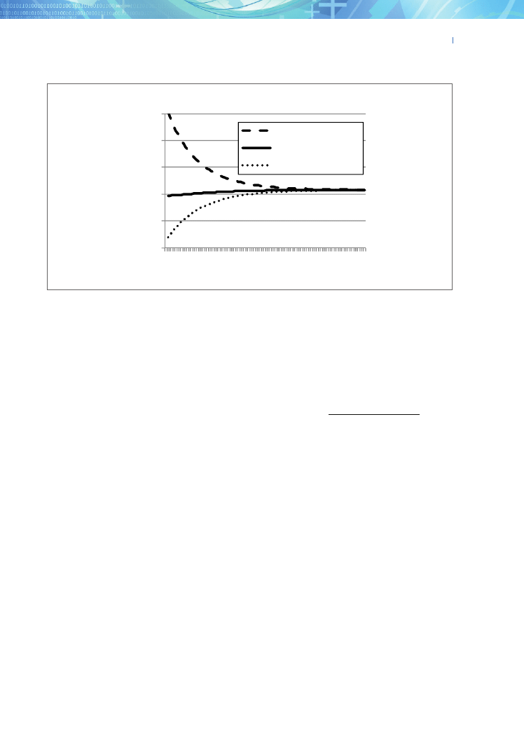
These rates are not equal, and hence the Polish econ-
omy is not yet on the balanced growth path. By (nu-
merically) solving the equation formed by equating
right-hand sides of equations (36) and (37), we obtain
the BGR in the baseline scenario. It is equal to 3.58%,
slightly higher than the average growth rate recorded
during the period 2000-2011. To depict the process
of convergence towards the balanced growth path, we
present a graph illustrating the trajectories of the above
growth rates in the baseline scenario.
6. Selected tax-cut scenarios in
Poland
Let us determine the effects of reducing various types
of taxes in the model calibrated for Poland. We con-
sider 2 types of scenarios:
a) reducing a given tax rate by 1 or 5 percentage
points (pp),
b) reducing all tax rates by 1 or 5 pp.
Table 2 contains the BGRs calculated under all of these
scenarios. In all cases, the economy grows more rap-
idly (on the balanced growth path) than in the baseline
scenario. To better visualize the long-term (welfare)
effect of reducing taxes, we also include numbers in-
dicating by how many percent GDP exceeds baseline
GDP after 30 years (in table 2, numbers in bold and
italics). These indicators are calculated as follows:
1
)
3 0
(
)
3 0
(
−
=
=
=
scenario
baseline
the
in
t
Y
scenario
selected
in
t
Y
years
3 0
after
gain
. (46)
In each scenario, the tax rates are reduced at
0
=
t
.
Unsurprisingly, the most favorable results are asso-
ciated with the largest tax cuts, i.e., the scenario of re-
ducing all tax rates by 5 pp. After 30 years, GDP would
be 11.9% higher than under the baseline scenario. Let
us analyze this specific scenario in greater depth. Table
3 summarizes selected structural macroeconomic in-
dicators under that scenario, relative to those in the
baseline scenario.
After lowering all tax rates by 5 pp, the overall tax
burden would decline from current 33% to 26.1% of
GDP, which would be similar to those currently ob-
served in the United States (approx. 25%), South Korea
(26%) and Japan (27%). The immediate effect of the re-
duction in taxes would be an increase in private sector
savings relative to GDP (from 20.7% to 22.4%), an in-
crease in investment (from 20% to 21.7% of GDP), and
finally, a rise in private expenditures on education. The
accelerated accumulation of both physical and human
capital would shift the economy to a higher balanced
Fig. 1. Convergence to the balanced growth path.
2,5%
3,0%
3,5%
4,0%
4,5%
5,0%
0 10 20 30 40 50 60 70 80 90 100
rate of growth of H
rate of growth of Y
rate of growth of K
Figure 1. Convergence to the balanced growth path.

338
Michał Konopczyński
10.5709/ce.1897-9254.149
DOI:
CONTEMPORARY ECONOMICS
Vol. 8
Issue 3
329-348
2014
1 pp reduction
5 pp reduction
L
τ
3.59%
3.66%
0.5%
2.5%
K
τ
3.59%
3.63%
0.3%
1.6%
H
τ
3.59%
3.66%
0.5%
2.5%
C
τ
3.61%
3.73%
0.9%
4.8%
reduction of all tax rates simultaneously
3.65%
3.95%
2.2%
11.9%
the BGR and structural indicators (%)
baseline scenario
reduction of all tax rates by 5 pp
the BGR
3.58
3.95 (the effect after 30 years= +11.9%)
Y
C /
61.9
67.0
Y
T /
33.0
26.1
Y
S /
20.7
22.4
Y
I
K
/
20.0
21.7
Y
G
E
/
5.8
5.8
Y
I
H
/
0.6
0.7
Table 2. Simulation results for Poland - different scenarios of tax cuts
Table 3. The scenario of simultaneously reducing all tax rates by 5 pp.
growth path. As a result, the BGR would increase by
approximately 0.38 percentage points.
It is worth noting that this scenario is associated
with significant structural changes in the economy. Re-
duced tax receipts, while maintaining a 15.5% share of
cash social transfers in GDP (primarily pensions) and
a 5.8% share of public expenditures on education in
GDP, would negatively affect public consumption ex-
penditures, i.e., national defense, public safety, health
care, public administration, environmental protec-
tion, etc. This gap would have to be (partially) offset
by increased consumption spending in the private sec-
tor. Thanks to the tax cuts, this would occur naturally.
Under the scenario presented in table 3, the share of
private consumption in GDP increases from 61.9% to
67.0%. Again, this would bring the Polish economy
structurally closer to the United States, where private
consumption is equal to approximately 70% of GDP.
7. Changing the structure of tax
revenue
The scenario of significant tax cuts presented in
the previous paragraph would be quite difficult
to achieve in practice due to the abovementioned
structural changes induced by the reduction in pub-
lic spending. It is tempting, therefore, to consider

Vizja Press&IT
www.ce.vizja.pl
339
How Taxes and Spending on Education Influence Economic Growth in Poland
The BGR and
structural
indicators
(%)
Baseline scenario
%
8 4
,
5
=
E
γ
%
0 2
,
2 5
=
γ
%
99
,
2
=
ψ
A
Increase in public
spending on education
by 1 pp of GDP
%
8 4
,
6
=
E
γ
B
Increase in private
savings by 1 pp of GDP
%
1 7
,
2 6
=
γ
%
99
,
2
=
ψ
C
Increase in private
spending on education
by 1 pp of GDP
%
2 1
,
2 6
=
γ
%
4 7
,
7
=
ψ
the BGR
3,58
3,89
GDP effect after 30 years
+9,4%
3,80
GDP effect after 30 years
+6,8%
3,90
GDP effect after 30 years
+9,5%
Y
C /
61,9
61,8
61,1
61,0
Y
T /
33,0
33,0
32,8
32,9
Y
S /
20,65
20,65
21,65
21,65
Y
I
K
/
20,04
20,04
21,01
20,04
Y
G
E
/
5,84
6,84
5,84
5,84
Y
I
H
/
0,62
0,62
0,65
1,62
Table 3. The scenario of simultaneously reducing all tax rates by 5 pp.
alternative scenarios with unchanged levels of taxa-
tion (and public spending) but a modified tax struc-
ture. Under this scenario, all three income tax rates
are reduced by 5 percentage points and the con-
sumption tax rate is increased, and hence the share
of taxes in GDP is identical to that in the baseline
scenario, i.e., 26.62% instead of 19.4%. The results
of the calculations reveal that such a change in the
tax structure would be neutral for the economy. Nei-
ther the BGR nor any of structural indicators (listed
in table 3) would change. Simply, in our model, the
structure of taxes is neutral – the important factor is
the level of taxation.
8. Selected scenarios of increasing
public and private spending on
education
In this section, 3 scenarios are presented:
A) the government increases public spending on edu-
cation by 1 pp of GDP at the expense of public con-
sumption.
B) private sector savings increase by 1 pp of GDP (at
the expense of individual consumption), with an
unchanged structure of investment expenditures
(i.e., an unchanged value of
ψ
). As a result, private
investment in physical and human capital would
increase by a total of 1 pp of GDP.
C) private sector savings increase by 1 pp of GDP (at
the expense of individual consumption), but addi-
tional savings are spent solely on education. (For
this purpose, the value of
ψ
has been appropriately
amended). In other words, private spending on ed-
ucation increases by 1 pp of GDP at the expense of
private consumption.
Table 4 presents the results.
With respect to the BGR, all three scenarios signifi-
cantly outperform the baseline scenario. However, the
effect of additional spending on education (scenarios
A and C) is stronger than the effect of a similar in-
crease in private savings, with additional resources be-
ing primarily spent on investments in physical capital
(97%). These simulations suggest that it is much more
preferable to spend additional money on education
rather than on physical capital. Moreover, from the
comparison of scenarios A and C, it follows that it is
relatively unimportant whether the additional funds
for education come from a reduction in public or pri-
vate consumption.
340
Michał Konopczyński
10.5709/ce.1897-9254.149
DOI:
CONTEMPORARY ECONOMICS
Vol. 8
Issue 3
329-348
2014
9. The optimal structure of private
investment
Clearly, investing in human capital (education) is of
crucial importance for economic growth. However,
in section 3, we were unable to analytically establish
the relationship between the BGR and the share pa-
rameter
ψ
(precisely, the share of private savings spent
on education). Now, using the baseline scenario as
a benchmark, we can calculate the BGR corresponding
to any value of
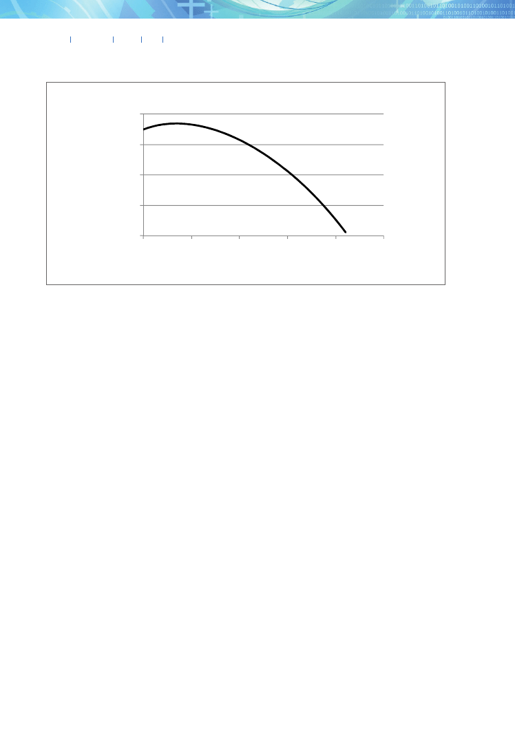
ψ
from 0% to 100%. Figure 2 pres-
ents the results. The BGR reaches a maximum (equal
to 3.695%) at
%
1 4
=
ψ
. According to Eurostat, at pres-
ent only 3% of private savings in Poland is spent on
education. Therefore, the current structure of private
investment in Poland is far from optimal. Households
should spend 14% of their savings on education, rather
than only 3%. However, in our view, it appears nearly
certain that private spending on education is underes-
timated in official statistics – a substantial share of it is
classified as consumption (e.g., the cost of accommo-
dation, travel, books, etc.).
Summary
In the long run, the economy is trending toward a dy-
namic equilibrium, characterized by so-called bal-
anced growth. We demonstrated that the equilibrium
is globally asymptotically stable. Despite the simplic-
ity of the model, the balanced growth rate (BGR) can
only be calculated numerically, as it requires solving
a complex, non-linear equation. On the one hand, the
BGR is an increasing function of the rate of private
savings, the rate of public transfers, and the rate of
public spending on education. On the other hand, the
BGR is a decreasing function of tax rates on labor, hu-
man capital and consumption. Finally, the relationship
between the BGR and the tax rate on capital income,
as well as the share coefficient (the percentage of pri-
vate savings invested in education), is ambiguous. It is
important to recall that this ambiguity is a property of
the theoretical model and implies that these relation-
ships are dependent on specific parameter values. In
other words, the relationship between the tax rate on
capital and the BGR can be positive or negative - it
depends on the parameter values. Therefore, this ques-
tion can only be addressed after establishing the values
of all parameters – as we do for Poland in the second
part of the paper. The central empirical conclusions re-
garding Poland can be summarized as follows. In the
period 2000-2011, economic growth in Poland was
primarily driven by a very rapid increase in the stock
of human capital (at a rate of 5% per annum) and only
secondarily by the accumulation of productive capital
Fig. 2. The BGR as a function of the
share parameter ψ
0,0%
1,0%
2,0%
3,0%
4,0%
0
0,2
0,4
0,6
0,8
1
BGR
Figure 2.The BGR as a function of the share parameter
ψ

Vizja Press&IT
www.ce.vizja.pl
341
How Taxes and Spending on Education Influence Economic Growth in Poland
(2.7% annually). Income taxes and consumption taxes
restrict economic growth to an equally burdensome
extent. Therefore, if the government must collect a cer-
tain amount of tax revenue, it is irrelevant what type of
tax will be used for that purpose.
Reducing income and consumption tax rates by 5
percentage points in Poland should increase annual
GDP growth by approximately 0.4 percentage points,
which after 30 years would entail a cumulative effect of
a 12% increase in GDP relative to a scenario assuming
current tax rates. Structurally, this scenario would bring
the Polish economy closer to such countries as the Unit-
ed States or South Korea, where the tax burden is sig-
nificantly lower (approximately 25% of GDP, whereas in
Poland it is 33%) and the share of individual consump-
tion is significantly higher (approximately 70% of GDP,
whereas the figure for Poland is approximately 62%).
Investing in human capital (education) is crucial to
economic growth. An increase in education expendi-
tures by 1 percentage point of GDP would have a similar
long-run effect as simultaneously reducing all tax rates
by 4 percentage points. The GDP growth rate would in-
crease by approximately 0.3 percentage points. Whether
the additional funding for education comes from a re-
duction in public or private consumption is irrelevant.
At present, households in Poland save approxi-
mately 21% of GDP, but only 3% of private savings
is spent on education, and 97% is invested in capital.
However, the optimal composition of savings, holding
all other parameters constant, is approximately 14% /
86%. Therefore, the current structure of private invest-
ment in Poland is far from the optimum. It is possible,
however, that private spending on education is under-
estimated in official statistics – a substantial share of
it is likely classified as consumption (e.g., the cost of
accommodation, travel, books, etc.).
Despite certain obvious simplifications, our analysis
provides qualitative and quantitative insights into the
negative effects of taxes and positive influence of educa-
tion on economic growth in Poland. It appears to capture
certain important ‘stylized facts’, especially the rapid ac-
cumulation of human capital over the past 20 years. Nev-
ertheless, one should recall that our model neglects cer-
tain important, though transitory, factors of growth. For
example, over the past decade, Poland experienced large
inflows of foreign capital, in the form of both FDI and
portfolio investment. However, a significant migration of
young persons from Poland to other EU countries was
observed. The growth effects of these two phenomena re-
main under investigation, but it is reasonable to contend
that they offset one another out to some extent.
References
Acemoglu, D. (2008). Introduction to Modern Eco-
nomic Growth. Princeton, NJ: Princeton Univer-
sity Press.
Agenor, P. R. (2007). Fiscal policy and endogenous
growth with public infrastructure. Oxford Eco-
nomic Papers, 60 (1), 57-87.
Arrazola, M., de Hevia, J. (2004). More on the estima-
tion of the human capital depreciation rate. Ap-
plied Economic Letters, 11 (3), 145-148.
Balistreri, E. J., McDaniel, C. A., Wong, E. V. (2003).
An estimation of US industry-level capital-labor
substitution elasticities: support for Cobb-Doug-
las. The North American Journal of Economics and
Finance, 14 (3), 343-356.
Barro, R. J. (1990). Government spending in a simple
model of economic growth. Journal of Political
Economy, 98 (5), 103-125.
Barro, R. J., Sala-i-Martin, X. (2004). Economic Growth
(2nd ed.). Cambrigde, MA: MIT Press
Campbell, J., Diamond, P., & Shoven, J. (2001). Estimat-
ing the Real Rate of Return on Stocks Over the Long
Term. Social Security Advisory Board, Washington.
Retrieved from: http://www.ssab.gov/publications/
financing/estimated%20rate%20of%20return.pdf
Cichy, K. (2008). Kapitał ludzki i postęp techniczny jako
determinanty wzrostu gospodarczego [Human capital
and technological progress as determinants of econom-
ic growth]. Warsaw: Instytut Wiedzy i Innowacji.
Dhont, T., Heylen, F. (2009). Employment and growth in
Europe and the US – the role of fiscal policy com-
position. Oxford Economic Papers, 61 (3), 538-565.
Elmendorf, D. W., Mankiw, N. G. (1998). Government
Debt (Working Papers No. 6470). National Bureau
of Economic Research.
Eurostat (2010). Taxation trends in the European Union
- Data for the EU Member States, Iceland and Nor-
way. Luxembourg: Publications Office of the Eu-
ropean Union. Retrieved from: http://ec.europa.
eu/taxation_customs/resources/documents/
taxation/gen_info/economic_analysis/tax_struc-
tures/2010/2010_full_text_en.pdf

342
Michał Konopczyński
10.5709/ce.1897-9254.149
DOI:
CONTEMPORARY ECONOMICS
Vol. 8
Issue 3
329-348
2014
Gordon, K., Tchilinguirian, H. (1998). Marginal Ef-
fective Tax Rates on Physical, Human and R&D
Capital (Working Papers No. ECO/WKP(98)12).
OECD Economic Department.
Heckman, J. J., Jacobs, B. (2010). Policies to Create
and Destroy Human Capital in Europe (Working
Papers No. 15742). National Bureau of Economic
Research.
Konopczyński, M. (2013). Fiscal policy within a com-
mon currency area – growth implications in the
light of neoclassical theory. Contemporary Eco-
nomics, 7 (3), 5-16.
Lee, Y., Gordon, R. (2005). Tax structure and econom-
ic growth. Journal of Public Economics, 89 (5-6),
1027-1043.
Mankiw, G. N., Romer, D., & Weil, D. N. (1992).
A Contribution to the Empirics of Economic
Growth. Quarterly Journal of Economics, 107 (2),
407-437.
Manuelli, R., Seshadri, A. (2005). Human Capital and
the Wealth of Nations (Meeting Papers No. 56). So-
ciety for Economic Dynamics.
Nehru, V., Dhareshwar, A. (1993). A new database on
physical capital stock: sources, methodology and
results. Revista de análisis económico, 8 (1), 37-59.
Próchniak, M. (2013). To What Extent Is the Institu-
tional Environment Responsible for Worldwide
Differences in Economic Development. Contem-
porary Economics, 7(3), 17-38.
Romer, P. M. (1986). Increasing returns and long-run
growth. Journal of Political Economy, 94 (5), 1002-
1037.
Turnovsky, S. J. (2009). Capital Accumulation and Eco-
nomic Growth in a Small Open Economy. Cam-
bridge, UK: Cambridge University Press.
Willman A. (2002). Euro Area Production Function
and Potential Output: A Supply Side System Ap-
proach (Working Papers No. 153). European Cen-
tral Bank.

Vizja Press&IT
www.ce.vizja.pl
343
How Taxes and Spending on Education Influence Economic Growth in Poland
Appendix
Proof of Proposition 1.
Dividing both sides of equation (11) by K and substi-
tuting (9), we obtain a formula for the growth rate of
productive capital:
K
K
Y
K
K
K
δ
γ
ψ
−
−
=
=
)
1
(
ˆ
,
(A1)
Similarly, by dividing both sides of equation (12) by H
and substituting (10), we obtain a formula for the rate
of human capital growth:
H
H
Y
H
H
H
δ
ψ γ
−
=
=
ˆ
,
(A2)
By assumption,
)
1
;
0
(
∈
ψ
and
)
1
;
0
(
∈
γ
. Thus, if
Y
K
ˆ
ˆ <
,
then capital grows more slowly than output, and con-
sequently, the ratio
K
Y
increases over time, which ac-
cording to (A1) implies that
Kˆ
also increases over time.
Conversely, if
Y
K
ˆ
ˆ >
, then capital grows more rapidly
than output, and hence the ratio
K
Y
, as well as
Kˆ
, will
decrease over time. Therefore, from equation (A1), it
follows that over time, the economy is converging to-
ward a balanced state, in which
Y
K
ˆ
ˆ =
. A similar con-
clusion follows from equation (A2): with the passage of
time, the economy is converging toward the balanced
state, in which
Y
H
ˆ
ˆ =
. Therefore, in the long term, the
economy converges toward the balanced growth path,
on which the following equality holds:
Y
H
K
ˆ
ˆ
ˆ
=
=
,
(A3)
From equations (A1) and (A2), if follows directly that
there exists exactly one such equilibrium (it is unique),
and it is globally asymptotically stable. To determine
the equilibrium, one must solve the system of equa-
tions (A3). First, note that from the equation (4), it
follows that:
H
K
Y
ˆ
)
1
(
ˆ
)
(
ˆ
β
α
β
α
−
−
+
+
=
,
(A4)
Thus, if
H
K
ˆ
ˆ =
, then
Y
H
K
ˆ
ˆ
ˆ
=
=
, and hence the system
of equations (A3) can be reduced to a single equation:
H
K
ˆ
ˆ =
. Unfortunately, except for certain special cases,
this equation cannot be solved analytically. To see why,
let us use equation (4) to write growth rates (A1) and
(A2) in the following equivalent form:
K
H
K
A
K
δ
γ
ψ
β
α
−
−
=
−
+
1
)
1
(
ˆ
,
(A5)
H
H
K
A
H
δ
ψ γ
β
α
−
=
+
ˆ
,
(A6)
We can treat the ratio
H
K
as a single variable (the un-
known). Then, from (A5) and (A6), it follows that the
equation
H
K
ˆ
ˆ =
can only be solved numerically, after
substituting certain values for all parameters. (Only in
special cases can this equation be solved analytically.
For example, if we set
3
1
=
=
β
α
, then this equation
can be transformed into a polynomial equation of the
fourth degree and solved analytically.) Nevertheless,
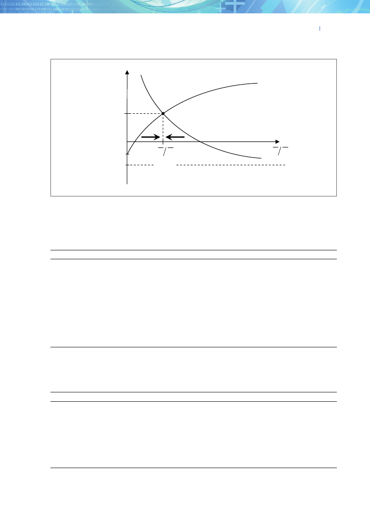
it is possible to “solve” it graphically, by graphing the
right-hand sides of equations (A5) and (A6). Strictly
speaking, we graph the rates of growth
Kˆ
and
Hˆ
as
functions of
H
K
. It is easy to show that the function
)
/
(
ˆ
H
K
K
is decreasing and strictly convex. Moreover,
+ ∞
→
+
→
0
/
ˆ
H
K
K
, and
K
H
K
K
δ
−
→
+ ∞
→
/
ˆ
. However,
the function
)
/
(
ˆ
H
K
H
is increasing, strictly concave,
H
H
K
H
δ
−
=
=
)
0
/
(
ˆ
, and
+ ∞
→
+ ∞
→
H
K
H
/
ˆ
. The graphs of
these functions are illustrated in figure A1. Due to the
properties of these functions, there is exactly one point
of intersection, i.e., there exists exactly one ratio
H
K
for which
H
K
ˆ
ˆ =
. The values of both functions at this
point determine the balanced growth rate (the BGR).
Figure A1 also indicates that the balanced state is
globally asymptotically stable. Notice that to the left
of the point of intersection of the graphs,
H
K
ˆ
ˆ >
, and
hence over time,
H
K
increases, which implies that
with the passage of time, the economy moves to the
right. However, to the right of the point of intersec-
tion of the graphs,
H
K
ˆ
ˆ <
, and hence over time,
H
K
decreases, which implies that with the passage of time,
the economy moves to the left. (The direction of mo-
tion is illustrated by the arrows in fig. A1.)
Notice that an increase in the value of the param-
eter
γ
and/or a decrease in the value of
K
δ
shifts the
graph of the function
)
/
(
ˆ
H
K
K
upwards. Similarly, an
increase in the value of the parameter
γ
and/or a de-
crease in the value of
H
δ
shifts the graph of the func-
tion
)
/
(
ˆ
H
K
H
upwards. Thus, the BGR is an increasing
function of
γ
and, simultaneously, a decreasing func-
tion of both rates of depreciation.
However, when the share parameter
ψ
increas-
es, the graph of
)
/
(
ˆ
H
K
K
shifts up, but the graph of
)
/
(
ˆ
H
K
H
simultaneously shifts down. Therefore, the
344
Michał Konopczyński
10.5709/ce.1897-9254.149
DOI:
CONTEMPORARY ECONOMICS
Vol. 8
Issue 3
329-348
2014
relationship between the BGR and
ψ
is ambiguous. It
can only be established numerically, after substituting
values for all parameters.
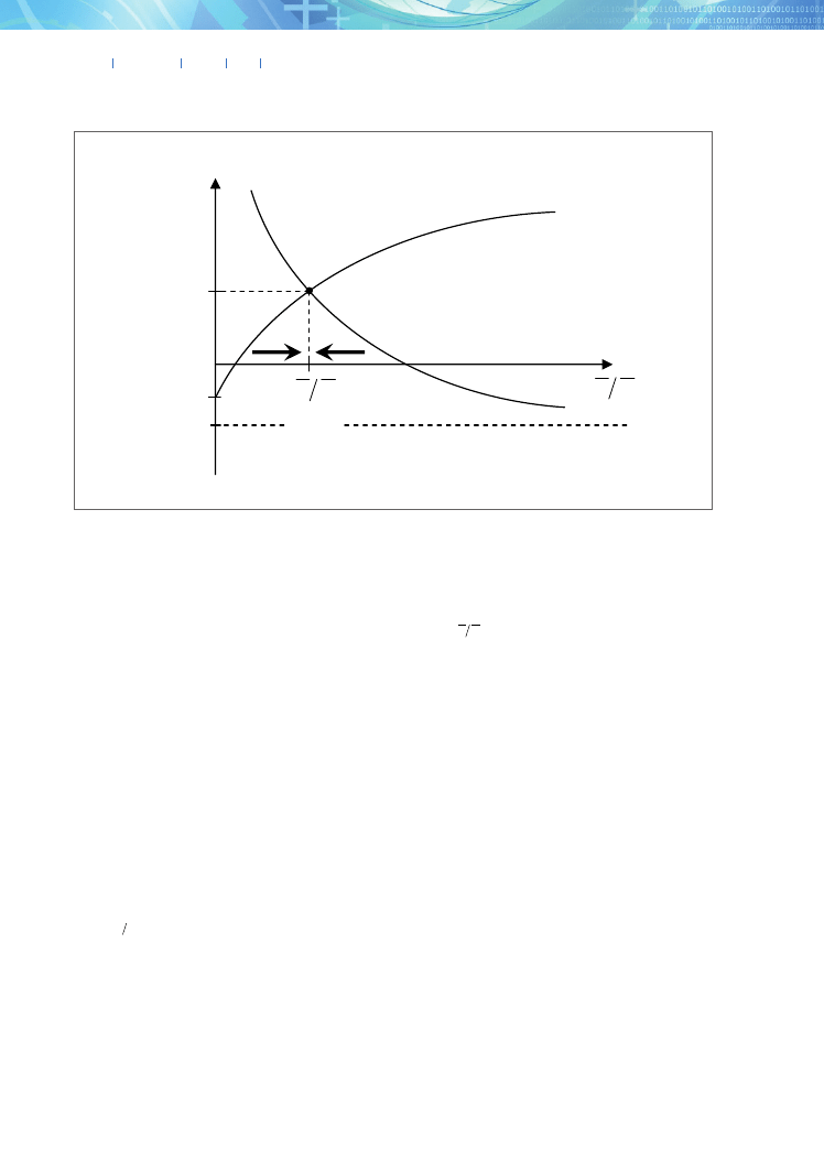
Proof of Proposition 2.
First, let us determine the signs of all expressions that
are marked with symbols
i
A
. Under the assumptions
adopted regarding the signs and the values of tax rates,
rates of savings, and other parameters, it can easily be
shown that:
0
,
,
,
6
5
3
2
>
A
A
A
A
,
0
4
<
A
and
1
2
<
A
,
1
6
<
A
,
(A7)
Similarly as above, let us graph the rates of growth
Kˆ
and
Hˆ
given by (36) and (37) as the functions of
H
K
. Using (A7) it is easy to prove that the function
)
/
(
ˆ
H
K
K
is decreasing and strictly convex. Moreover,
+ ∞
→
+
→
0
/
ˆ
H
K
K
, and
4
/
ˆ
A
K
H
K
→
+ ∞
→
. However, the
function
)
/
(
ˆ
H
K
H
is increasing, strictly concave,
H
H
K
H
δ
−
=
=
)
0
/
(
ˆ
, and
+ ∞
→
+ ∞
→
H
K
H
/
ˆ
. The graphs
of these functions are illustrated in figure A2. Due
to the properties of these functions, there is exactly
one point of intersection, i.e., there exists exactly one
ratio
H
K
for which
H
K
ˆ
ˆ =
. The values of both func-
tions at this point determine the balanced growth rate
(the BGR). The balanced state is globally asymptoti-
cally stable, which is illustrated in figure A2. In equi-
librium
H
K
ˆ
ˆ =
, which together with (4), implies that
H
K
Y
ˆ
ˆ
ˆ
=
=
.
Sensitivity of the results to the K/Y ratio
Due to lack of suitable statistics, the ratio of
Y
K /
for
Poland was calibrated based on the average value for
22 OECD countries, which is equal to 3.0. However,
in certain OECD countries, the
Y
K /
ratio is higher,
while it is lower in others. This section presents the
most important results of the paper; we set the ratio
of
Y
K /
for Poland at the level of 3.3 or 2.7, instead of
3.0 (as we do in the main text). Tables 2A – 4A are the
counterparts of tables 2 – 4 if we set
3
.
3
/ =
Y
K
. Simi-
larly, tables 2B – 4B are the counterparts of tables 2 – 4
if we set
7
.
2
/ =
Y
K
. The general conclusion is that the
results are very insensitive to the initial value of
Y
K /
.
All welfare gains – as measured by the GDP effect after
30 years – are very similar to the results obtained in
the main text.
Fig. A1. Graphs of the functions
)
/
(
ˆ
H
K
K
and
)
/
(
ˆ
H
K
H
in the private economy
BGR
H
K
0
H
δ
−
K
δ
−
H
K ˆ
,
ˆ
Hˆ
Kˆ
H
K
Figure A1. Graphs of the functions
)
/
(
ˆ
H
K
K
and
)
/
(
ˆ
H
K
H
in the private economy
Vizja Press&IT
www.ce.vizja.pl
345
How Taxes and Spending on Education Influence Economic Growth in Poland
Fig. A2. Graphs of the functions
)
/
(
ˆ
H
K
K
and
)
/
(
ˆ
H
K
H
in the economy with the government
BGR
H
K
0
H
δ
−
4
A
H
K ˆ
,
ˆ
Hˆ
Kˆ
H
K
Figure A2. Graphs of the functions
)
/
(
ˆ
H
K
K
and
)
/
(
ˆ
H
K
H
in the economy with the government
1 pp reduction
5 pp reduction
L
τ
3.54%
3.60%
0.5%
2.4%
K
τ
3.53%
3.58%
0.3%
1.5%
H
τ
3.54%
3.60%
0.5%
2.4%
C
τ
3.55%
3.68%
0.9%
4.6%
reduction of all tax rates simultaneously
3.60%
3.90%
2.2%
11.6%
the BGR and structural indicators (%)
baseline scenario
reduction of all tax rates by 5 pp
the BGR
3.52
3.90 (the effect after 30 years= +11.6%)
Y
C /
61.7
66.9
Y
T /
33.2
26.3
Y
S /
20.6
22.3
Y
I
K
/
20.0
21.6
Y
G
E
/
5.8
5.8
Y
I
H
/
0.6
0.7
Table 2A. Simulation results for Poland - different tax-cut scenarios,
3
.
3
/ =
Y
K
.
Table 2A. The scenario of simultaneously reducing all tax rates by 5 pp,
3
.
3
/ =
Y
K
.

346
Michał Konopczyński
10.5709/ce.1897-9254.149
DOI:
CONTEMPORARY ECONOMICS
Vol. 8
Issue 3
329-348
2014
The BGR and structural
indicators
(%)
Baseline scenario
%
8 4
.
5
=
E
γ
%
0 2
.
2 5
=
γ
%
99
.
2
=
ψ
A
Increase in public
spending on education
by 1 pp of GDP
%
8 4
.
6
=
E
γ
B
Increase in private
savings by 1 pp of GDP
%
1 7
.
2 6
=
γ
%
99
.
2
=
ψ
C
Increase in private
spending on education
by 1 pp of GDP
%
2 1
.
2 6
=
γ
%
4 7
.
7
=
ψ
the BGR
3.52
3.84
GDP effect
after 30 years
+9.8%
3.74
GDP effect
after 30 years
+6.6%
3.84
GDP effect
after 30 years
+9.9%
Y
C /
61.7
61.7
60.9
60.8
Y
T /
33.2
33.3
33.0
33.1
Y
S /
20.6
20.6
21.6
21.6
Y
I
K
/
20.0
20.0
21.0
20.0
Y
G
E
/
5.84
6.84
5.84
5.84
Y
I
H
/
0.62
0.62
0.65
1.62
1 pp reduction
5 pp reduction
L
τ
3.50%
3.57%
0.5%
2.5%
K
τ
3.50%
3.54%
0.3%
1.7%
H
τ
3.50%
3.57%
0.5%
2.5%
C
τ
3.52%
3.64%
0.9%
4.8%
reduction of all tax rates simultaneously
3.56%
3.86%
2.3%
12.1%
the BGR and structural indicators (%)
baseline scenario
reduction of all tax rates by 5 pp
the BGR
3.49
3.86 (the effect after 30 years= +12.1%)
Y
C /
62.1
67.2
Y
T /
32.7
25.8
Y
S /
20.7
22.4
Y
I
K
/
20.1
21.8
Y
G
E
/
5.84
5.84
Y
I
H
/
0.62
0.67
Table 4A. Scenarios of increasing public and private spending on education,
3
.
3
/ =
Y
K
Table 2B. Simulation results for Poland – different tax-cut scenarios,
7
.
2
/ =
Y
K
.
Table 3B. The scenario of simultaneously reducing all tax rates by 5 pp,
7
.
2
/ =
Y
K
.

Vizja Press&IT
www.ce.vizja.pl
347
How Taxes and Spending on Education Influence Economic Growth in Poland
The BGR and structural
indicators
(%)
Baseline scenario
%
8 4
.
5
=
E
γ
%
0 2
.
2 5
=
γ
%
99
.
2
=
ψ
A
Increase in public
spending on education
by 1 pp of GDP
%
8 4
.
6
=
E
γ
B
Increase in private
savings by 1 pp of GDP
%
1 7
.
2 6
=
γ
%
99
.
2
=
ψ
C
Increase in private
spending on education
by 1 pp of GDP
%
2 1
.
2 6
=
γ
%
4 7
.
7
=
ψ
the BGR
3.49
3.80
GDP effect after 30
years +8.6%
3.70
GDP effect after 30
years +6.9%
3.81
GDP effect after 30
years +8.8%
Y
C /
62.1
62.0
61.3
61.2
Y
T /
32.7
32.8
32.5
32.6
Y
S /
20.7
20.70
21.7
21.7
Y
I
K
/
20.1
20.1
21.1
20.1
Y
G
E
/
5.84
6.84
5.84
5.84
Y
I
H
/
0.62
0.62
0.65
1.62
Table 4B. Scenarios of increasing public and private spending on education,
7
.
2
/ =
Y
K
.

348
Michał Konopczyński
10.5709/ce.1897-9254.149
DOI:
CONTEMPORARY ECONOMICS
Vol. 8
Issue 3
329-348
2014
Wyszukiwarka
Podobne podstrony:
Kwiek, Marek Social Perceptions versus Economic Returns of the Higher Education The Bologna Process
The influence of British imperialism and racism on relationships to Indians
How to Analyze People on Sight, by Elsie Lincoln Benedict and Ralph Paine Benedict
Text which I chose is strongly connected with the economy and conditions on the market
1998 The influence of sugar beet fibre, guar gum and inulin on
Influence of extraction parameters and medium on efficiency
Master Your Fears How to Triumph Over Your Worries and Get on with Your Life Mantesh
How to set alarm to save picture and video on the SD card
United Nations Conference on Trade and Development Economic Development in Africa (2007)
How to configure VLANS on DFL Series Firewall and Layer 2 Managed Switch
Anglik Tom and Sheila on board the ship
The Great?pression Summary and?fects on the People
Gemes Freud and Nietzsche on Sublimation
33 437 452 Primary Carbides in Spincast HSS for Hot Rolls and Effect on Oxidation
Adolf Hitler His Life and?fect on History
więcej podobnych podstron