
SOLUTIONS TO PROBLEMS
ELEMENTARY
LINEAR ALGEBRA
K. R. MATTHEWS
DEPARTMENT OF MATHEMATICS
UNIVERSITY OF QUEENSLAND
First Printing,
1991

CONTENTS
PROBLEMS 1.6
............................................ 1
PROBLEMS 2.4
............................................ 12
PROBLEMS 2.7
............................................ 18
PROBLEMS 3.6
............................................ 32
PROBLEMS 4.1
............................................ 45
PROBLEMS 5.8
............................................ 58
PROBLEMS 6.3
............................................ 69
PROBLEMS 7.3
............................................ 83
PROBLEMS 8.8
............................................ 91
i

SECTION
1
.6
2. (i)
· 0 0 0
2 4 0
¸
R
1
↔ R
2
· 2 4 0
0 0 0
¸
R
1
→
1
2
R
1
· 1 2 0
0 0 0
¸
;
(ii)
· 0 1 3
1 2 4
¸
R
1
↔ R
2
· 1 2 4
0 1 3
¸
R
1
→ R
1
− 2R
2
· 1 0 −2
0 1
3
¸
;
(iii)
1 1 1
1 1 0
1 0 0
R
2
→ R
2
− R
1
R
3
→ R
3
− R
1
1
1
0
0
0
−1
0
−1 −1
R
1
→ R
1
+ R
3
R
3
→ −R
3
R
2
↔ R
3
1 0
0
0 1
1
0 0
−1
R
2
→ R
2
+ R
3
R
3
→ −R
3
1 0 0
0 1 0
0 0 1
;
(iv)
2 0 0
0 0 0
−4 0 0
R
3
→ R
3
+ 2R
1
R
1
→
1
2
R
1
1 0 0
0 0 0
0 0 0
.
3. (a)
1
1
1
2
2
3
−1
8
1
−1 −1 −8
R
2
→ R
2
− 2R
1
R
3
→ R
3
− R
1
1
1
1
2
0
1
−3
4
0
−2 −2 −10
R
1
→ R
1
− R
2
R
3
→ R
3
+ 2R
2
1 0
4
−2
0 1
−3
4
0 0
−8 −2
R
3
→
−1
8
R
3
1 0
4 2
0 1
−3 4
0 0
1
1
4
R
1
→ R
1
− 4R
3
R
2
→ R
2
+ 3R
3
1 0 0
−3
0 1 0
19
4
0 0 1
1
4
.
The augmented matrix has been converted to reduced row–echelon form
and we read off the unique solution x =
−3, y =
19
4
, z =
1
4
.
(b)
1
1
−1
2 10
3
−1
7
4
1
−5
3
−15 −6
9
R
2
→ R
2
− 3R
1
R
3
→ R
3
+ 5R
1
1
1
−1
2
10
0
−4
10
−2 −29
0
8
−20
4
59
R
3
→ R
3
+ 2R
2
1
1
−1
2
10
0
−4 10 −2 −29
0
0
0
0
1
.
From the last matrix we see that the original system is inconsistent.
1

(c)
3
−1
7 0
2
−1
4
1
2
1
−1
1 1
6
−4 10 3
R
1
↔ R
3
1
−1
1 1
2
−1
4
1
2
3
−1
7 0
6
−4 10 3
R
2
→ R
2
− 2R
1
R
3
→ R
3
− 3R
1
R
4
→ R
4
− 6R
1
1
−1 1
1
0
1 2
−3
2
0
2 4
−3
0
2 4
−3
R
1
→ R
1
+ R
2
R
4
→ R
4
− R
3
R
3
→ R
3
− 2R
2
1 0 3
−1
2
0 1 2
−3
2
0 0 0
0
0 0 0
0
.
The augmented matrix has been converted to reduced row–echelon form
and we read off the complete solution x =
−
1
2
− 3z, y = −
3
2
− 2z, with z
arbitrary.
4.
2
−1
3 a
3
1
−5 b
−5 −5 21 c
R
2
→ R
2
− R
1
2
−1
3
a
1
2
−8 b − a
−5 −5 21
c
R
1
↔ R
2
1
2
−8 b − a
2
−1
3
a
−5 −5 21
c
R
2
→ R
2
− 2R
1
R
3
→ R
3
+ 5R
1
1
2
−8
b
− a
0
−5
19
−2b + 3a
0
5
−19 5b − 5a + c
R
3
→ R
3
+ R
2
R
2
→
−1
5
R
2
1 2
−8
b
− a
0 1
−19
5
2b−3a
5
0 0
0 3b
− 2a + c
R
1
→ R
1
− 2R
2
1 0
−2
5
(b+a)
5
0 1
−19
5
2b−3a
5
0 0
0 3b
− 2a + c
.
From the last matrix we see that the original system is inconsistent if
3b
− 2a + c 6= 0. If 3b − 2a + c = 0, the system is consistent and the solution
is
x =
(b + a)
5
+
2
5
z, y =
(2b
− 3a)
5
+
19
5
z,
where z is arbitrary.
5.
1
1 1
t
1 t
1 + t 2 3
R
2
→ R
2
− tR
1
R
3
→ R
3
− (1 + t)R
1
1
1
1
0 1
− t
0
0 1
− t 2 − t
R
3
→ R
3
− R
2
1
1
1
0 1
− t
0
0
0
2
− t
= B.
2

Case 1. t
6= 2. No solution.
Case 2. t = 2. B =
1
0 1
0
−1 0
0
0 0
→
1 0 1
0 1 0
0 0 0
.
We read off the unique solution x = 1, y = 0.
6. Method 1.
−3
1
1
1
1
−3
1
1
1
1
−3
1
1
1
1
−3
R
1
→ R
1
− R
4
R
2
→ R
2
− R
4
R
3
→ R
3
− R
4
−4
0
0
4
0
−4
0
4
0
0
−4
4
1
1
1
−3
→
1 0 0
−1
0 1 0
−1
0 0 1
−1
1 1 1
−3
R
4
→ R
4
− R
3
− R
2
− R
1
1 0 0
−1
0 1 0
−1
0 0 1
−1
0 0 0
0
.
Hence the given homogeneous system has complete solution
x
1
= x
4
, x
2
= x
4
, x
3
= x
4
,
with x
4
arbitrary.
Method 2. Write the system as
x
1
+ x
2
+ x
3
+ x
4
= 4x
1
x
1
+ x
2
+ x
3
+ x
4
= 4x
2
x
1
+ x
2
+ x
3
+ x
4
= 4x
3
x
1
+ x
2
+ x
3
+ x
4
= 4x
4
.
Then it is immediate that any solution must satisfy x
1
= x
2
= x
3
= x
4
.
Conversely, if x
1
, x
2
, x
3
, x
4
satisfy x
1
= x
2
= x
3
= x
4
, we get a solution.
7.
· λ − 3
1
1
λ
− 3
¸
R
1
↔ R
2
·
1
λ
− 3
λ
− 3
1
¸
R
2
→ R
2
− (λ − 3)R
1
· 1
λ
− 3
0
−λ
2
+ 6λ
− 8
¸
= B.
3

Case 1:
−λ
2
+ 6λ
− 8 6= 0. That is −(λ − 2)(λ − 4) 6= 0 or λ 6= 2, 4. Here B is
row equivalent to
· 1 0
0 1
¸
:
R
2
→
1
−λ
2
+6λ−8
R
2
· 1 λ − 3
0
1
¸
R
1
→ R
1
− (λ − 3)R
2
· 1 0
0 1
¸
.
Hence we get the trivial solution x = 0, y = 0.
Case 2: λ = 2. Then B =
· 1 −1
0
0
¸
and the solution is x = y, with y arbitrary.
Case 3: λ = 4. Then B =
· 1 1
0 0
¸
and the solution is x =
−y, with y arbitrary.
8.
· 3
1 1
1
5
−1 1 −1
¸
R
1
→
1
3
R
1
· 1
1
3
1
3
1
3
5
−1 1 −1
¸
R
2
→ R
2
− 5R
1
· 1
1
3
1
3
1
3
0
−
8
3
−
2
3
−
8
3
¸
R
2
→
−3
8
R
2
· 1
1
3
1
3
1
3
0 1
1
4
1
¸
R
1
→ R
1
−
1
3
R
2
· 1 0
1
4
0
0 1
1
4
1
¸
.
Hence the solution of the associated homogeneous system is
x
1
=
−
1
4
x
3
, x
2
=
−
1
4
x
3
− x
4
,
with x
3
and x
4
arbitrary.
9.
A =
1
− n
1
· · ·
1
1
1
− n · · ·
1
...
...
· · ·
...
1
1
· · · 1 − n
R
1
→ R
1
− R
n
R
2
→ R
2
− R
n
...
R
n−1
→ R
n−1
− R
n
−n
0
· · ·
n
0
−n · · ·
n
...
... ···
...
1
1
· · · 1 − n
→
1 0
· · ·
−1
0 1
· · ·
−1
... ... ···
...
1 1
· · · 1 − n
R
n
→ R
n
− R
n−1
· · · − R
1
1 0
· · · −1
0 1
· · · −1
... ... ··· ...
0 0
· · ·
0
.
4

The last matrix is in reduced row–echelon form.
Consequently the homogeneous system with coefficient matrix A has the
solution
x
1
= x
n
, x
2
= x
n
, . . . , x
n−1
= x
n
,
with x
n
arbitrary.
Alternatively, writing the system in the form
x
1
+
· · · + x
n
= nx
1
x
1
+
· · · + x
n
= nx
2
...
x
1
+
· · · + x
n
= nx
n
shows that any solution must satisfy nx
1
= nx
2
=
· · · = nx
n
, so x
1
= x
2
=
· · · = x
n
. Conversely if x
1
= x
n
, . . . , x
n−1
= x
n
, we see that x
1
, . . . , x
n
is a
solution.
10. Let A =
· a b
c d
¸
and assume that ad
− bc 6= 0.
Case 1: a
6= 0.
· a b
c d
¸
R
1
→
1
a
R
1
· 1
b
a
c d
¸
R
2
→ R
2
− cR
1
· 1
b
a
0
ad−bc
a
¸
R
2
→
a
ad−bc
R
2
· 1
b
a
0 1
¸
R
1
→ R
1
−
b
a
R
2
· 1 0
0 1
¸
.
Case 2: a = 0. Then bc
6= 0 and hence c 6= 0.
A =
· 0 b
c d
¸
R
1
↔ R
2
·
c d
0 b
¸
→
· 1
d
c
0 1
¸
→
· 1 0
0 1
¸
.
So in both cases, A has reduced row–echelon form equal to
· 1 0
0 1
¸
.
11. We simplify the augmented matrix of the system using row operations:
1
2
−3
4
3
−1
5
2
4
1 a
2
− 14 a + 2
R
2
→ R
2
− 3R
1
R
3
→ R
3
− 4R
1
1
2
−3
4
0
−7
14
−10
0
−7 a
2
− 2 a − 14
5

R
3
→ R
3
− R
2
R
2
→
−1
7
R
2
R
1
→ R
1
− 2R
2
1 2
−3
4
0 1
−2
10
7
0 0 a
2
− 16 a − 4
R
1
→ R
1
− 2R
2
1 0
1
8
7
0 1
−2
10
7
0 0 a
2
− 16 a − 4
.
Denote the last matrix by B.
Case 1: a
2
− 16 6= 0. i.e. a 6= ±4. Then
R
3
→
1
a
2
−16
R
3
R
1
→ R
1
− R
3
R
2
→ R
2
+ 2R
3
1 0 0
8a+25
7(a+4)
0 1 0
10a+54
7(a+4)
0 0 1
1
a+4
and we get the unique solution
x =
8a + 25
7(a + 4)
, y =
10a + 54
7(a + 4)
, z =
1
a + 4
.
Case 2: a =
−4. Then B =
1 0
1
8
7
0 1
−2
10
7
0 0
0
−8
, so our system is inconsistent.
Case 3: a = 4. Then B =
1 0
1
8
7
0 1
−2
10
7
0 0
0
0
. We read off that the system is
consistent, with complete solution x =
8
7
− z, y =
10
7
+ 2z, where z is
arbitrary.
12. We reduce the augmented array of the system to reduced row–echelon
form:
1 0 1 0 1
0 1 0 1 1
1 1 1 1 0
0 0 1 1 0
R
3
→ R
3
+ R
1
1 0 1 0 1
0 1 0 1 1
0 1 0 1 1
0 0 1 1 0
R
3
→ R
3
+ R
2
1 0 1 0 1
0 1 0 1 1
0 0 0 0 0
0 0 1 1 0
R
1
→ R
1
+ R
4
R
3
↔ R
4
1 0 0 1 1
0 1 0 1 1
0 0 1 1 0
0 0 0 0 0
.
6

The last matrix is in reduced row–echelon form and we read off the solution
of the corresponding homogeneous system:
x
1
=
−x
4
− x
5
= x
4
+ x
5
x
2
=
−x
4
− x
5
= x
4
+ x
5
x
3
=
−x
4
= x
4
,
where x
4
and x
5
are arbitrary elements of
Z
2
. Hence there are four solutions:
x
1
x
2
x
3
x
4
x
5
0
0
0
0
0
1
1
0
0
1
1
1
1
1
0
0
0
1
1
1
.
13. (a) We reduce the augmented matrix to reduced row–echelon form:
2 1 3 4
4 1 4 1
3 1 2 0
R
1
→ 3R
1
1 3 4 2
4 1 4 1
3 1 2 0
R
2
→ R
2
+ R
1
R
3
→ R
3
+ 2R
1
1 3 4 2
0 4 3 3
0 2 0 4
R
2
→ 4R
2
1 3 4 2
0 1 2 2
0 2 0 4
R
1
→ R
1
+ 2R
2
R
3
→ R
3
+ 3R
2
1 0 3 1
0 1 2 2
0 0 1 0
R
1
→ R
1
+ 2R
3
R
2
→ R
2
+ 3R
3
1 0 0 1
0 1 0 2
0 0 1 0
.
Consequently the system has the unique solution x = 1, y = 2, z = 0.
(b) Again we reduce the augmented matrix to reduced row–echelon form:
2 1 3 4
4 1 4 1
1 1 0 3
R
1
↔ R
3
1 1 0 3
4 1 4 1
2 1 3 4
R
2
→ R
2
+ R
1
R
3
→ R
3
+ 3R
1
1 1 0 3
0 2 4 4
0 4 3 3
R
2
→ 3R
2
1 1 0 3
0 1 2 2
0 4 3 3
7

R
1
→ R
1
+ 4R
2
R
3
→ R
3
+ R
2
1 0 3 1
0 1 2 2
0 0 0 0
.
We read off the complete solution
x = 1
− 3z = 1 + 2z
y = 2
− 2z = 2 + 3z,
where z is an arbitrary element of
Z
5
.
14. Suppose that (α
1
, . . . , α
n
) and (β
1
, . . . , β
n
) are solutions of the system of
linear equations
n
X
j=1
a
ij
x
j
= b
i
,
1
≤ i ≤ m.
Then
n
X
j=1
a
ij
α
j
= b
i
and
n
X
j=1
a
ij
β
j
= b
i
for 1
≤ i ≤ m.
Let γ
i
= (1
− t)α
i
+ tβ
i
for 1
≤ i ≤ m. Then (γ
1
, . . . , γ
n
) is a solution of
the given system. For
n
X
j=1
a
ij
γ
j
=
n
X
j=1
a
ij
{(1 − t)α
j
+ tβ
j
}
=
n
X
j=1
a
ij
(1
− t)α
j
+
n
X
j=1
a
ij
tβ
j
= (1
− t)b
i
+ tb
i
= b
i
.
15. Suppose that (α
1
, . . . , α
n
) is a solution of the system of linear equations
n
X
j=1
a
ij
x
j
= b
i
,
1
≤ i ≤ m.
(1)
Then the system can be rewritten as
n
X
j=1
a
ij
x
j
=
n
X
j=1
a
ij
α
j
,
1
≤ i ≤ m,
8

or equivalently
n
X
j=1
a
ij
(x
j
− α
j
) = 0,
1
≤ i ≤ m.
So we have
n
X
j=1
a
ij
y
j
= 0,
1
≤ i ≤ m.
where x
j
− α
j
= y
j
. Hence x
j
= α
j
+ y
j
, 1
≤ j ≤ n, where (y
1
, . . . , y
n
) is a
solution of the associated homogeneous system. Conversely if (y
1
, . . . , y
n
) is
a solution of the associated homogeneous system and x
j
= α
j
+ y
j
, 1
≤ j ≤
n, then reversing the argument shows that (x
1
, . . . , x
n
) is a solution of the
system 1 .
16. We simplify the augmented matrix using row operations, working towards
row–echelon form:
1 1
−1 1
1
a 1
1 1
b
3 2
0 a 1 + a
R
2
→ R
2
− aR
1
R
3
→ R
3
− 3R
1
1
1
−1
1
1
0 1
− a 1 + a 1 − a b − a
0
−1
3
a
− 3 a − 2
R
2
↔ R
3
R
2
→ −R
2
1
1
−1
1
1
0
1
−3
3
− a 2 − a
0 1
− a 1 + a 1 − a b − a
R
3
→ R
3
+ (a
− 1)R
2
1 1
−1
1
1
0 1
−3
3
− a
2
− a
0 0 4
− 2a (1 − a)(a − 2) −a
2
+ 2a + b
− 2
= B.
Case 1: a
6= 2. Then 4 − 2a 6= 0 and
B
→
1 1
−1
1
1
0 1
−3 3 − a
2
− a
0 0
1
a−1
2
−a
2
+2a+b−2
4−2a
.
Hence we can solve for x, y and z in terms of the arbitrary variable w.
Case 2: a = 2. Then
B =
1 1
−1 1
1
0 1
−3 1
0
0 0
0 0 b
− 2
.
9

Hence there is no solution if b
6= 2. However if b = 2, then
B =
1 1
−1 1 1
0 1
−3 1 0
0 0
0 0 0
→
1 0
2 0 1
0 1
−3 1 0
0 0
0 0 0
and we get the solution x = 1
− 2z, y = 3z − w, where w is arbitrary.
17. (a) We first prove that 1 + 1 + 1 + 1 = 0. Observe that the elements
1 + 0,
1 + 1,
1 + a,
1 + b
are distinct elements of F by virtue of the cancellation law for addition. For
this law states that 1 + x = 1 + y
⇒ x = y and hence x 6= y ⇒ 1 + x 6= 1 + y.
Hence the above four elements are just the elements 0, 1, a, b in some
order. Consequently
(1 + 0) + (1 + 1) + (1 + a) + (1 + b) = 0 + 1 + a + b
(1 + 1 + 1 + 1) + (0 + 1 + a + b) = 0 + (0 + 1 + a + b),
so 1 + 1 + 1 + 1 = 0 after cancellation.
Now 1 + 1 + 1 + 1 = (1 + 1)(1 + 1), so we have x
2
= 0, where x = 1 + 1.
Hence x = 0. Then a + a = a(1 + 1) = a
· 0 = 0.
Next a + b = 1. For a + b must be one of 0, 1, a, b. Clearly we can’t have
a + b = a or b; also if a + b = 0, then a + b = a + a and hence b = a; hence
a + b = 1. Then
a + 1 = a + (a + b) = (a + a) + b = 0 + b = b.
Similarly b + 1 = a. Consequently the addition table for F is
+
0
1
a
b
0
0
1
a
b
1
1
0
b
a
a
a
b
0
1
b
b
a
1
0
.
We now find the multiplication table. First, ab must be one of 1, a, b;
however we can’t have ab = a or b, so this leaves ab = 1.
10

Next a
2
= b. For a
2
must be one of 1, a, b; however a
2
= a
⇒ a = 0 or
a = 1; also
a
2
= 1
⇒ a
2
− 1 = 0 ⇒ (a − 1)(a + 1) = 0 ⇒ (a − 1)
2
= 0
⇒ a = 1;
hence a
2
= b. Similarly b
2
= a. Consequently the multiplication table for F
is
× 0 1 a b
0
0
0
0
0
1
0
1
a
b
a
0
a
b
1
b
0 b
1
a
.
(b) We use the addition and multiplication tables for F :
A =
1 a b a
a b b 1
1 1 1 a
R
2
→ R
2
+ aR
1
R
3
→ R
3
+ R
1
1 a b a
0 0 a a
0 b a 0
R
2
↔ R
3
1 a b a
0 b a 0
0 0 a a
R
2
→ aR
2
R
3
→ bR
3
1 a b a
0 1 b 0
0 0 1 1
R
1
↔ R
1
+ aR
2
1 0 a a
0 1 b 0
0 0 1 1
R
1
→ R
1
+ aR
3
R
2
→ R
2
+ bR
3
1 0 0 0
0 1 0 b
0 0 1 1
.
The last matrix is in reduced row–echelon form.
11

Section
2
.4
2. Suppose B =
a b
c d
e f
and that AB = I
2
. Then
· −1 0 1
0
1 0
¸
a b
c d
e f
=
· 1 0
0 1
¸
=
· −a + e −b + f
c + e
d + f
¸
.
Hence
−a + e = 1
c + e = 0
, −
b + f = 0
d + f = 1
;
e = a + 1
c =
−e = −(a + 1)
,
f = b
d = 1
− f = 1 − b
;
B =
a
b
−a − 1 1 − b
a + 1
b
.
Next,
(BA)
2
B = (BA)(BA)B = B(AB)(AB) = BI
2
I
2
= BI
2
= B
4. Let p
n
denote the statement
A
n
=
(3
n
−1)
2
A +
(3−3
n
)
2
I
2
.
Then p
1
asserts that A =
(3−1)
2
A +
(3−3)
2
I
2
, which is true. So let n
≥ 1 and
assume p
n
. Then from (1),
A
n+1
= A
· A
n
= A
n
(3
n
−1)
2
A +
(3−3
n
)
2
I
2
o
=
(3
n
−1)
2
A
2
+
(3−3
n
)
2
A
=
(3
n
−1)
2
(4A
− 3I
2
) +
(3−3
n
)
2
A =
(3
n
−1)4+(3−3
n
)
2
A +
(3
n
−1)(−3)
2
I
2
=
(4·3
n
−3
n
)−1
2
A +
(3−3
n+1
)
2
I
2
=
(3
n+1
−1)
2
A +
(3−3
n+1
)
2
I
2
.
Hence p
n+1
is true and the induction proceeds.
12

5. The equation x
n+1
= ax
n
+ bx
n−1
is seen to be equivalent to
· x
n+1
x
n
¸
=
· a b
1 0
¸ ·
x
n
x
n−1
¸
or
X
n
= AX
n−1
,
where X
n
=
· x
n+1
x
n
¸
and A =
· a b
1 0
¸
. Then
X
n
= A
n
X
0
if n
≥ 1. Hence by Question 3,
· x
n+1
x
n
¸
=
½ (3
n
− 1)
2
A +
(3
− 3
n
)
2
I
2
¾ · x
1
x
0
¸
=
½ (3
n
− 1)
2
· 4 −3
1
0
¸
+
·
3−3
n
2
0
0
3−3
n
2
¸¾ · x
1
x
0
¸
=
(3
n
− 1)2 +
3−3
n
2
(3
n
− 1)(−3)
3
n
−1
2
3−3
n
2
· x
1
x
0
¸
Hence, equating the (2, 1) elements gives
x
n
=
(3
n
− 1)
2
x
1
+
(3
− 3
n
)
2
x
0
if n
≥ 1
7. Note: λ
1
+ λ
2
= a + d and λ
1
λ
2
= ad
− bc.
Then
(λ
1
+ λ
2
)k
n
− λ
1
λ
2
k
n−1
= (λ
1
+ λ
2
)(λ
n−1
1
+ λ
n−2
1
λ
2
+
· · · + λ
1
λ
n−2
2
+ λ
n−1
2
)
−λ
1
λ
2
(λ
n−2
1
+ λ
n−3
1
λ
2
+
· · · + λ
1
λ
n−3
2
+ λ
n−2
2
)
= (λ
n
1
+ λ
n−1
1
λ
2
+
· · · + λ
1
λ
n−1
2
)
+(λ
n−1
1
λ
2
+
· · · + λ
1
λ
n−1
2
+ λ
n
2
)
−(λ
n−1
1
λ
2
+
· · · + λ
1
λ
n−1
2
)
= λ
n
1
+ λ
n−1
1
λ
2
+
· · · + λ
1
λ
n−1
2
+ λ
n
2
= k
n+1
13

If λ
1
= λ
2
, we see
k
n
= λ
n−1
1
+ λ
n−2
1
λ
2
+
· · · + λ
1
λ
n−2
2
+ λ
n−1
2
= λ
n−1
1
+ λ
n−2
1
λ
1
+
· · · + λ
1
λ
n−2
1
+ λ
n−1
1
= nλ
n−1
1
If λ
1
6= λ
2
, we see that
(λ
1
− λ
2
)k
n
= (λ
1
− λ
2
)(λ
n−1
1
+ λ
n−2
1
λ
2
+
· · · + λ
1
λ
n−2
2
+ λ
n−1
2
)
= λ
n
1
+ λ
n−1
1
λ
2
+
· · · + λ
1
λ
n−1
2
−(λ
n−1
1
λ
2
+
· · · + λ
1
λ
n−1
2
+ λ
n
2
)
= λ
n
1
− λ
n
2
.
Hence k
n
=
λ
n
1
−λ
n
2
λ
1
−λ
2
.
We have to prove
A
n
= k
n
A
− λ
1
λ
2
k
n−1
I
2
.
∗
n=1:
A
1
= A; also k
1
A
− λ
1
λ
2
k
0
I
2
= k
1
A
− λ
1
λ
2
0I
2
= A.
Let n
≥ 1 and assume equation ∗ holds. Then
A
n+1
= A
n
· A = (k
n
A
− λ
1
λ
2
k
n−1
I
2
)A
= k
n
A
2
− λ
1
λ
2
k
n−1
A.
Now A
2
= (a + d)A
− (ad − bc)I
2
= (λ
1
+ λ
2
)A
− λ
1
λ
2
I
2
. Hence
A
n+1
= k
n
(λ
1
+ λ
2
)A
− λ
1
λ
2
I
2
− λ
1
λ
2
k
n−1
A
=
{k
n
(λ
1
+ λ
2
)
− λ
1
λ
2
k
n−1
}A − λ
1
λ
2
k
n
I
2
= k
n+1
A
− λ
1
λ
2
k
n
I
2
,
and the induction goes through.
8. Here λ
1
, λ
2
are the roots of the polynomial x
2
− 2x − 3 = (x − 3)(x + 1).
So we can take λ
1
= 3, λ
2
=
−1. Then
k
n
=
3
n
− (−1)
n
3
− (−1)
=
3
n
+ (
−1)
n+1
4
.
14
Hence
A
n
=
½ 3
n
+ (
−1)
n+1
4
¾
A
− (−3)
½ 3
n−1
+ (
−1)
n
4
¾
I
2
=
3
n
+ (
−1)
n+1
4
· 1 2
2 1
¸
+ 3
½ 3
n−1
+ (
−1)
n
4
¾ · 1 0
0 1
¸
,
which is equivalent to the stated result.
9. In terms of matrices, we have
· F
n+1
F
n
¸
=
· 1 1
1 0
¸ ·
F
n
F
n−1
¸
for n
≥ 1.
· F
n+1
F
n
¸
=
· 1 1
1 0
¸
n
· F
1
F
0
¸
=
· 1 1
1 0
¸
n
· 1
0
¸
.
Now λ
1
, λ
2
are the roots of the polynomial x
2
− x + 1 here.
Hence λ
1
=
1+
√
5
2
and λ
2
=
1−
√
5
2
and
k
n
=
³
1+
√
5
2
´
n−1
−
³
1−
√
5
2
´
n−1
1+
√
5
2
−
³
1−
√
5
2
´
=
³
1+
√
5
2
´
n−1
−
³
1−
√
5
2
´
n−1
√
5
.
Hence
A
n
= k
n
A
− λ
1
λ
2
k
n−1
I
2
= k
n
A
− k
n−1
I
2
So
· F
n+1
F
n
¸
= (k
n
A
− k
n−1
I
2
)
· 1
0
¸
= k
n
· 1
1
¸
− k
n−1
· 1
0
¸
=
· k
n
− k
n−1
k
n
¸
.
Hence
F
n
= k
n
=
³
1+
√
5
2
´
n−1
−
³
1−
√
5
2
´
n−1
√
5
.
15

10. From Question 5, we know that
· x
n
y
n
¸
=
· 1 r
1 1
¸
n
· a
b
¸
.
Now by Question 7, with A =
· 1 r
1 1
¸
,
A
n
= k
n
A
− λ
1
λ
2
k
n−1
I
2
= k
n
A
− (1 − r)k
n−1
I
2
,
where λ
1
= 1 +
√
r and λ
2
= 1
−
√
r are the roots of the polynomial x
2
−
2x + (1
− r) and
k
n
=
λ
n
1
− λ
n
2
2
√
r
.
Hence
· x
n
y
n
¸
= (k
n
A
− (1 − r)k
n−1
I
2
)
· a
b
¸
=
µ· k
n
k
n
r
k
n
k
n
¸
−
· (1 − r)k
n−1
0
0
(1
− r)k
n−1
¸¶ · a
b
¸
=
· k
n
− (1 − r)k
n−1
k
n
r
k
n
k
n
− (1 − r)k
n−1
¸ · a
b
¸
=
· a(k
n
− (1 − r)k
n−1
) + bk
n
r
ak
n
+ b(k
n
− (1 − r)k
n−1
)
¸
.
Hence, in view of the fact that
k
n
k
n−1
=
λ
n
1
− λ
n
2
λ
n−1
1
− λ
n−1
2
=
λ
n
1
(1
− {
λ
2
λ
1
}
n
)
λ
n−1
1
(1
− {
λ
2
λ
1
}
n−1
)
→ λ
1
,
as n
→ ∞,
we have
· x
n
y
n
¸
=
a(k
n
− (1 − r)k
n−1
) + bk
n
r
ak
n
+ b(k
n
− (1 − r)k
n−1
)
=
a(
k
n
k
n−1
− (1 − r)) + b
k
n
k
n−1
r
a
k
n
k
n−1
+ b(
k
n
k
n−1
− (1 − r))
→
a(λ
1
− (1 − r)) + bλ
1
r
aλ
1
+ b(λ
1
− (1 − r))
16
=
a(
√
r + r) + b(1 +
√
r)r
a(1 +
√
r) + b(
√
r + r)
=
√
r
{a(1 +
√
r) + b(1 +
√
r)
√
r
}
a(1 +
√
r) + b(
√
r + r)
=
√
r.
17

Section
2
.7
1. [A
|I
2
] =
·
1 4
−3 1
¯
¯
¯
¯
1 0
0 1
¸
R
2
→ R
2
+ 3R
1
· 1 4
0 13
¯
¯
¯
¯
1 0
3 1
¸
R
2
→
1
13
R
2
· 1 4
0 1
¯
¯
¯
¯
1
0
3/13 1/13
¸
R
1
→ R
1
− 4R
2
· 1 0
0 1
¯
¯
¯
¯
1/13
−4/13
3/13
1/13
¸
.
Hence A is non–singular and A
−1
=
· 1/13 −4/13
3/13
1/13
¸
.
Moreover
E
12
(
−4)E
2
(1/13)E
21
(3)A = I
2
,
so
A
−1
= E
12
(
−4)E
2
(1/13)E
21
(3).
Hence
A =
{E
21
(3)
}
−1
{E
2
(1/13)
}
−1
{E
12
(
−4)}
−1
= E
21
(
−3)E
2
(13)E
12
(4).
2. Let D = [d
ij
] be an m
× m diagonal matrix and let A = [a
jk
] be an m
× n
matrix. Then
(DA)
ik
=
n
X
j=1
d
ij
a
jk
= d
ii
a
ik
,
as d
ij
= 0 if i
6= j. It follows that the ith row of DA is obtained by multiplying
the ith row of A by d
ii
.
Similarly, post–multiplication of a matrix by a diagonal matrix D re-
sults in a matrix whose columns are those of A, multiplied by the respective
diagonal elements of D.
In particular,
diag (a
1
, . . . , a
n
)diag (b
1
, . . . , b
n
) = diag (a
1
b
1
, . . . , a
n
b
n
),
as the left–hand side can be regarded as pre–multiplication of the matrix
diag (b
1
, . . . , b
n
) by the diagonal matrix diag (a
1
, . . . , a
n
).
Finally, suppose that each of a
1
, . . . , a
n
is non–zero. Then a
−1
1
, . . . , a
−1
n
all exist and we have
diag (a
1
, . . . , a
n
)diag (a
−1
1
, . . . , a
−1
n
) = diag (a
1
a
−1
1
, . . . , a
n
a
−1
n
)
= diag (1, . . . , 1) = I
n
.
18

Hence diag (a
1
, . . . , a
n
) is non–singular and its inverse is diag (a
−1
1
, . . . , a
−1
n
).
Next suppose that a
i
= 0. Then diag (a
1
, . . . , a
n
) is row–equivalent to a
matix containing a zero row and is hence singular.
3. [A
|I
3
] =
0 0 2
1 2 6
3 7 9
¯
¯
¯
¯
¯
¯
1 0 0
0 1 0
0 0 1
R
1
↔ R
2
1 2 6 0 1 0
0 0 2 1 0 0
3 7 9 0 0 1
R
3
→ R
3
− 3R
1
1 2
6 0
1 0
0 0
2 1
0 0
0 1
−9 0 −3 1
R
2
↔ R
3
1 2
6 0
1 0
0 1
−9 0 −3 1
0 0
2 1
0 0
R
3
→
1
2
R
3
1 2
6
0
1 0
0 1
−9
0
−3 1
0 0
1 1/2
0 0
R
1
→ R
1
− 2R
2
1 0
24
0
7
−2
0 1
−9
0
−3
1
0 0
1 1/2
0
0
R
1
→ R
1
− 24R
3
R
2
→ R
2
+ 9R
3
1 0 0
−12
7
−2
0 1 0
9/2
−3
1
0 0 1
1/2
0
0
.
Hence A is non–singular and A
−1
=
−12
7
−2
9/2
−3
1
1/2
0
0
.
Also
E
23
(9)E
13
(
−24)E
12
(
−2)E
3
(1/2)E
23
E
31
(
−3)E
12
A = I
3
.
Hence
A
−1
= E
23
(9)E
13
(
−24)E
12
(
−2)E
3
(1/2)E
23
E
31
(
−3)E
12
,
so
A = E
12
E
31
(3)E
23
E
3
(2)E
12
(2)E
13
(24)E
23
(
−9).
4.
A =
1
2
k
3
−1
1
5
3
−5
→
1
2
k
0
−7
1
− 3k
0
−7 −5 − 5k
→
1
2
k
0
−7
1
− 3k
0
0
−6 − 2k
= B.
Hence if
−6 − 2k 6= 0, i.e. if k 6= −3, we see that B can be reduced to I
3
and hence A is non–singular.
19

If k =
−3, then B =
1
2
−3
0
−7 10
0
0
0
= B and consequently A is singular,
as it is row–equivalent to a matrix containing a zero row.
5. E
21
(2)
·
1
2
−2 −4
¸
=
· 1 2
0 0
¸
. Hence, as in the previous question,
·
1
2
−2 −4
¸
is singular.
6. Starting from the equation A
2
− 2A + 13I
2
= 0, we deduce
A(A
− 2I
2
) =
−13I
2
= (A
− 2I
2
)A.
Hence AB = BA = I
2
, where B =
−1
13
(A
− 2I
2
). Consequently A is non–
singular and A
−1
= B.
7. We assume the equation A
3
= 3A
2
− 3A + I
3
.
(ii) A
4
= A
3
A = (3A
2
− 3A + I
3
)A = 3A
3
− 3A
2
+ A
= 3(3A
2
− 3A + I
3
)
− 3A
2
+ A = 6A
2
− 8A + 3I
3
.
(iii) A
3
− 3A
2
+ 3A = I
3
. Hence
A(A
2
− 3A + 3I
3
) = I
3
= (A
2
− 3A + 3I
3
)A.
Hence A is non–singular and
A
−1
= A
2
− 3A + 3I
3
=
−1 −3
1
2
4
−1
0
1
0
.
8. (i) If B
3
= 0 then
(I
n
− B)(I
n
+ B + B
2
) = I
n
(I
n
+ B + B
2
)
− B(I
n
+ B + B
2
)
= (I
n
+ B + B
2
)
− (B + B
2
+ B
3
)
= I
n
− B
3
= I
n
− 0 = I
n
.
Similarly (I
n
+ B + B
2
)(I
n
− B) = I
n
.
Hence A = I
n
− B is non–singular and A
−1
= I
n
+ B + B
2
.
20

It follows that the system AX = b has the unique solution
X = A
−1
b = (I
n
+ B + B
2
)b = b + Bb + B
2
b.
(ii) Let B =
0 r s
0 0 t
0 0 0
. Then B
2
=
0 0 rt
0 0 0
0 0 0
and B
3
= 0. Hence
from the preceding question
(I
3
− B)
−1
= I
3
+ B + B
2
=
1 0 0
0 1 0
0 0 1
+
0 r s
0 0 t
0 0 0
+
0 0 rt
0 0 0
0 0 0
=
1 r s + rt
0 1
t
0 0
1
.
9. (i) Suppose that A
2
= 0. Then if A
−1
exists, we deduce that A
−1
(AA) =
A
−1
0, which gives A = 0 and this is a contradiction, as the zero matrix is
singular. We conclude that A does not have an inverse.
(ii). Suppose that A
2
= A and that A
−1
exists. Then
A
−1
(AA) = A
−1
A,
which gives A = I
n
. Equivalently, if A
2
= A and A
6= I
n
, then A does not
have an inverse.
10. The system of linear equations
x + y
− z = a
z = b
2x + y + 2z = c
is equivalent to the matrix equation AX = B, where
A =
1 1
−1
0 0
1
2 1
2
,
X =
x
y
z
,
B =
a
b
c
.
21

By Question 7, A
−1
exists and hence the system has the unique solution
X =
−1 −3
1
2
4
−1
0
1
0
a
b
c
=
−a − 3b + c
2a + 4b
− c
b
.
Hence x =
−a − 3b + c, y = 2a + 4b − c, z = b.
12.
A = E
3
(2)E
14
E
42
(3) = E
3
(2)E
14
1 0 0 0
0 1 0 0
0 0 1 0
0 3 0 1
= E
3
(2)
0 3 0 1
0 1 0 0
0 0 1 0
1 0 0 0
=
0 3 0 1
0 1 0 0
0 0 2 0
1 0 0 0
.
Also
A
−1
= (E
3
(2)E
14
E
42
(3))
−1
= (E
42
(3))
−1
E
−1
14
(E
3
(2))
−1
= E
42
(
−3)E
14
E
3
(1/2)
= E
42
(
−3)E
14
1 0
0
0
0 1
0
0
0 0 1/2 0
0 0
0
1
= E
42
(
−3)
0 0
0
1
0 1
0
0
0 0 1/2 0
1 0
0
0
=
0
0
0
1
0
1
0
0
0
0
1/2 0
1
−3
0
0
.
13. (All matrices in this question are over
Z
2
.)
22

(a)
1 1 0 1
0 0 1 1
1 1 1 1
1 0 0 1
¯
¯
¯
¯
¯
¯
¯
¯
1 0 0 0
0 1 0 0
0 0 1 0
0 0 0 1
→
1 1 0 1
0 0 1 1
0 0 1 0
0 1 0 0
¯
¯
¯
¯
¯
¯
¯
¯
1 0 0 0
0 1 0 0
1 0 1 0
1 0 0 1
→
1 1 0 1
0 1 0 0
0 0 1 0
0 0 1 1
¯
¯
¯
¯
¯
¯
¯
¯
1 0 0 0
1 0 0 1
1 0 1 0
0 1 0 0
→
1 0 0 1
0 1 0 0
0 0 1 0
0 0 0 1
¯
¯
¯
¯
¯
¯
¯
¯
0 0 0 1
1 0 0 1
1 0 1 0
1 1 1 0
→
1 0 0 0
0 1 0 0
0 0 1 0
0 0 0 1
¯
¯
¯
¯
¯
¯
¯
¯
1 1 1 1
1 0 0 1
1 0 1 0
1 1 1 0
.
Hence A is non–singular and
A
−1
=
1 1 1 1
1 0 0 1
1 0 1 0
1 1 1 0
.
(b) A =
1 1 0 1
0 1 1 1
1 0 1 0
1 1 0 1
R
4
→ R
4
+ R
1
1 1 0 1
0 1 1 1
1 0 1 0
0 0 0 0
, so A is singular.
14.
(a)
1 1 1
−1 1 0
2 0 0
¯
¯
¯
¯
¯
¯
1 0 0
0 1 0
0 0 1
R
3
→
1
2
R
3
R
1
→ R
1
− R
3
R
2
→ R
2
+ R
3
R
1
↔ R
3
1 0 0
0 1 0
0 1 1
¯
¯
¯
¯
¯
¯
0 0
1/2
0 1
1/2
1 0
−1/2
R
3
→ R
3
− R
2
1 0 0
0 1 0
0 0 1
¯
¯
¯
¯
¯
¯
0
0 1/2
0
1 1/2
1
−1 −1
.
Hence A
−1
exists and
A
−1
=
0
0 1/2
0
1 1/2
1
−1 −1
.
23

(b)
2 2 4
1 0 1
0 1 0
¯
¯
¯
¯
¯
¯
1 0 0
0 1 0
0 0 1
R
1
→ R
1
− 2R
2
R
1
↔ R
2
R
2
↔ R
3
1 0 1
0 1 0
0 2 2
¯
¯
¯
¯
¯
¯
0
1 0
0
0 1
1
−2 0
R
3
→ R
3
− 2R
2
1 0 1
0 1 0
0 0 2
¯
¯
¯
¯
¯
¯
0
1
0
0
0
1
1
−2 −2
R
3
→
1
2
R
3
1 0 1
0 1 0
0 0 1
¯
¯
¯
¯
¯
¯
0
1
0
0
0
1
1/2
−1 −1
R
1
→ R
1
− R
3
1 0 0
0 1 0
0 0 1
¯
¯
¯
¯
¯
¯
−1/2
2
1
0
0
1
1/2
−1 −1
.
Hence A
−1
exists and
A
−1
=
−1/2
2
1
0
0
1
1/2
−1 −1
.
(c)
4 6
−3
0 0
7
0 0
5
R
2
→
1
7
R
2
R
3
→
1
5
R
3
4 6
−3
0 0
1
0 0
1
R
3
→ R
3
− R
2
4 6
−3
0 0
1
0 0
0
.
Hence A is singular by virtue of the zero row.
(d)
2
0 0
0
−5 0
0
0 7
¯
¯
¯
¯
¯
¯
1 0 0
0 1 0
0 0 1
R
1
→
1
2
R
1
R
2
→
−1
5
R
2
R
3
→
1
7
R
3
1 0 0
0 1 0
0 0 1
¯
¯
¯
¯
¯
¯
1/2
0
0
0
−1/5
0
0
0 1/7
.
Hence A
−1
exists and A
−1
= diag (1/2,
−1/5, 1/7).
(Of course this was also immediate from Question 2.)
(e)
1 2 4 6
0 1 2 0
0 0 1 2
0 0 0 2
¯
¯
¯
¯
¯
¯
¯
¯
1 0 0 0
0 1 0 0
0 0 1 0
0 0 0 1
R
1
→ R
1
− 2R
2
1 0 0 6
0 1 2 0
0 0 1 2
0 0 0 2
¯
¯
¯
¯
¯
¯
¯
¯
1
−2 0 0
0
1 0 0
0
0 1 0
0
0 0 1
R
2
→ R
2
− 2R
3
1 0 0
6
0 1 0
−4
0 0 1
2
0 0 0
2
¯
¯
¯
¯
¯
¯
¯
¯
1
−2
0 0
0
1
−2 0
0
0
1 0
0
0
0 1
24

R
1
→ R
1
− 3R
4
R
2
→ R
2
+ 2R
4
R
3
→ R
3
− R
4
R
4
→
1
2
R
4
1 0 0 0
0 1 0 0
0 0 1 0
0 0 0 1
¯
¯
¯
¯
¯
¯
¯
¯
1
−2
0
−3
0
1
−2
2
0
0
1
−1
0
0
0 1/2
.
Hence A
−1
exists and
A
−1
=
1
−2
0
−3
0
1
−2
2
0
0
1
−1
0
0
0 1/2
.
(f)
1 2 3
4 5 6
5 7 9
R
2
→ R
2
− 4R
1
R
3
→ R
3
− 5R
1
1
2
3
0
−3 −6
0
−3 −6
R
3
→ R
3
− R
2
1
2
3
0
−3 −6
0
0
0
.
Hence A is singular by virtue of the zero row.
15. Suppose that A is non–singular. Then
AA
−1
= I
n
= A
−1
A.
Taking transposes throughout gives
(AA
−1
)
t
= I
t
n
= (A
−1
A)
t
(A
−1
)
t
A
t
= I
n
= A
t
(A
−1
)
t
,
so A
t
is non–singular and (A
t
)
−1
= (A
−1
)
t
.
16. Let A =
· a b
c d
¸
, where ad
− bc = 0. Then the equation
A
2
− (a + d)A + (ad − bc)I
2
= 0
reduces to A
2
− (a + d)A = 0 and hence A
2
= (a + d)A. From the last
equation, if A
−1
exists, we deduce that A = (a + d)I
2
, or
· a b
c d
¸
=
· a + d
0
0
a + d
¸
.
Hence a = a + d, b = 0, c = 0, d = a + d and a = b = c = d = 0, which
contradicts the assumption that A is non–singular.
25

17.
A =
1
a b
−a
1 c
−b −c 1
R
2
→ R
2
+ aR
1
R
3
→ R
3
+ bR
1
1
a
b
0 1 + a
2
c + ab
0 ab
− c 1 + b
2
R
2
→
1
1+a
2
R
2
1
a
b
0
1
c+ab
1+a
2
0 ab
− c 1 + b
2
R
3
→ R
3
− (ab − c)R
2
1 a
b
0 1
c+ab
1+a
2
0 0 1 + b
2
+
(c−ab)(c+ab)
1+a
2
= B.
Now
1 + b
2
+
(c
− ab)(c + ab)
1 + a
2
= 1 + b
2
+
c
2
− (ab)
2
1 + a
2
=
1 + a
2
+ b
2
+ c
2
1 + a
2
6= 0.
Hence B can be reduced to I
3
using four more row operations and conse-
quently A is non–singular.
18. The proposition is clearly true when n = 1. So let n
≥ 1 and assume
(P
−1
AP )
n
= P
−1
A
n
P . Then
(P
−1
AP )
n+1
= (P
−1
AP )
n
(P
−1
AP )
= (P
−1
A
n
P )(P
−1
AP )
= P
−1
A
n
(P P
−1
)AP
= P
−1
A
n
IAP
= P
−1
(A
n
A)P
= P
−1
A
n+1
P
and the induction goes through.
19. Let A =
· 2/3 1/4
1/3 3/4
¸
and P =
·
1 3
−1 4
¸
. Then P
−1
=
1
7
· 4 −3
1
1
¸
.
We then verify that P
−1
AP =
· 5/12 0
0
1
¸
. Then from the previous ques-
tion,
P
−1
A
n
P = (P
−1
AP )
n
=
· 5/12 0
0
1
¸
n
=
· (5/12)
n
0
0
1
n
¸
=
· (5/12)
n
0
0
1
¸
.
26

Hence
A
n
= P
· (5/12)
n
0
0
1
¸
P
−1
=
·
1 3
−1 4
¸ · (5/12)
n
0
0
1
¸ 1
7
· 4 −3
1
1
¸
=
1
7
·
(5/12)
n
3
−(5/12)
n
4
¸ · 4 −3
1
1
¸
=
1
7
·
4(5/12)
n
+ 3
(
−3)(5/12)
n
+ 3
−4(5/12)
n
+ 4
3(5/12)
n
+ 4
¸
=
1
7
· 3 3
4 4
¸
+
1
7
(5/12)
n
·
4
−3
−4
3
¸
.
Notice that A
n
→
1
7
· 3 3
4 4
¸
as n
→ ∞. This problem is a special case of a
more general result about Markov matrices.
20. Let A =
· a b
c d
¸
be a matrix whose elements are non–negative real
numbers satisfying
a
≥ 0, b ≥ 0, c ≥ 0, d ≥ 0, a + c = 1 = b + d.
Also let P =
· b
1
c
−1
¸
and suppose that A
6= I
2
.
(i) det P =
−b − c = −(b + c). Now b + c ≥ 0. Also if b + c = 0, then we
would have b = c = 0 and hence d = a = 1, resulting in A = I
2
. Hence
det P < 0 and P is non–singular.
Next,
P
−1
AP =
−1
b + c
· −1 −1
−c
b
¸ · a b
c d
¸ · b
1
c
−1
¸
=
−1
b + c
·
−a − c
−b − d
−ac + bc −cb + bd
¸ · b
1
c
−1
¸
=
−1
b + c
·
−1
−1
−ac + bc −cb + bd
¸ · b
1
c
−1
¸
=
−1
b + c
·
−b − c
0
(
−ac + bc)b + (−cb + bd)c −ac + bc + cb − bd
¸
.
Now
−acb + b
2
c
− c
2
b + bdc =
−cb(a + c) + bc(b + d)
=
−cb + bc = 0.
27

Also
−(a + d − 1)(b + c) = −ab − ac − db − dc + b + c
=
−ac + b(1 − a) + c(1 − d) − bd
=
−ac + bc + cb − bd.
Hence
P
−1
AP =
−1
b + c
· −(b + c)
0
0
−(a + d − 1)(b + c)
¸
=
· 1
0
0 a + d
− 1
¸
.
(ii) We next prove that if we impose the extra restriction that A
6=
· 0 1
1 0
¸
,
then
|a + d − 1| < 1. This will then have the following consequence:
A = P
· 1
0
0 a + d
− 1
¸
P
−1
A
n
= P
· 1
0
0 a + d
− 1
¸
n
P
−1
= P
· 1
0
0 (a + d
− 1)
n
¸
P
−1
→ P
· 1 0
0 0
¸
P
−1
=
· b
1
c
−1
¸ · 1 0
0 0
¸
−1
b + c
· −1 −1
−c
b
¸
=
−1
b + c
· b 0
c 0
¸ · −1 −1
−c
b
¸
=
−1
b + c
· −b −b
−c −c
¸
=
1
b + c
· b b
c c
¸
,
where we have used the fact that (a + d
− 1)
n
→ 0 as n → ∞.
We first prove the inequality
|a + d − 1| ≤ 1:
a + d
− 1 ≤ 1 + d − 1 = d ≤ 1
a + d
− 1 ≥ 0 + 0 − 1 = −1.
28

Next, if a + d
− 1 = 1, we have a + d = 2; so a = 1 = d and hence c = 0 = b,
contradicting our assumption that A
6= I
2
. Also if a + d
− 1 = −1, then
a + d = 0; so a = 0 = d and hence c = 1 = b and hence A =
· 0 1
1 0
¸
.
22. The system is inconsistent: We work towards reducing the augmented
matrix:
1 2
1 1
3 5
¯
¯
¯
¯
¯
¯
4
5
12
R
2
→ R
2
− R
1
R
3
→ R
3
− 3R
1
1
2
0
−1
0
−1
¯
¯
¯
¯
¯
¯
4
1
0
R
3
→ R
3
− R
2
1
2
0
−1
0
0
¯
¯
¯
¯
¯
¯
4
1
−1
.
The last row reveals inconsistency.
The system in matrix form is AX = B, where
A =
1 2
1 1
3 5
,
X =
· x
y
¸
,
B =
4
5
12
.
The normal equations are given by the matrix equation
A
t
AX = A
t
B.
Now
A
t
A =
· 1 1 3
2 1 5
¸
1 2
1 1
3 5
=
· 11 18
18 30
¸
A
t
B =
· 1 1 3
2 1 5
¸
4
5
12
=
· 45
73
¸
.
Hence the normal equations are
11x + 18y = 45
18x + 30y = 73.
29

These may be solved, for example, by Cramer’s rule:
x =
¯
¯
¯
¯
45 18
73 30
¯
¯
¯
¯
¯
¯
¯
¯
11 18
18 30
¯
¯
¯
¯
=
36
6
= 6
y =
¯
¯
¯
¯
11 45
18 73
¯
¯
¯
¯
¯
¯
¯
¯
11 18
18 30
¯
¯
¯
¯
=
−7
6
.
23. Substituting the coordinates of the five points into the parabola equation
gives the following equations:
a = 0
a + b + c
=
0
a + 2b + 4c
=
−1
a + 3b + 9c
=
4
a + 4b + 16c
=
8.
The associated normal equations are given by
5
10
30
10
30
100
30 100 354
a
b
c
=
11
42
160
,
which have the solution a = 1/5, b =
−2, c = 1.
24. Suppose that A is symmetric, i.e. A
t
= A and that AB is defined. Then
(B
t
AB)
t
= B
t
A
t
(B
t
)
t
= B
t
AB,
so B
t
AB is also symmetric.
25. Let A be m
× n and B be n × m, where m > n. Then the homogeneous
system BX = 0 has a non–trivial solution X
0
, as the number of unknowns
is greater than the number of equations. Then
(AB)X
0
= A(BX
0
) = A0 = 0
30

and the m
× m matrix AB is therefore singular, as X
0
6= 0.
26. (i) Let B be a singular n
× n matrix. Then BX = 0 for some non–zero
column vector X. Then (AB)X = A(BX) = A0 = 0 and hence AB is also
singular.
(ii) Suppose A is a singular n
× n matrix. Then A
t
is also singular and
hence by (i) so is B
t
A
t
= (AB)
t
. Consequently AB is also singular
31

Section 3.6
1. (a) Let S be the set of vectors [x, y] satisfying x = 2y. Then S is a vector
subspace of
R
2
. For
(i) [0, 0]
∈ S as x = 2y holds with x = 0 and y = 0.
(ii) S is closed under addition. For let [x
1
, y
1
] and [x
2
, y
2
] belong to S.
Then x
1
= 2y
1
and x
2
= 2y
2
. Hence
x
1
+ x
2
= 2y
1
+ 2y
2
= 2(y
1
+ y
2
)
and hence
[x
1
+ x
2
, y
1
+ y
2
] = [x
1
, y
1
] + [x
2
, y
2
]
belongs to S.
(iii) S is closed under scalar multiplication. For let [x, y]
∈ S and t ∈ R.
Then x = 2y and hence tx = 2(ty). Consequently
[tx, ty] = t[x, y]
∈ S.
(b) Let S be the set of vectors [x, y] satisfying x = 2y and 2x = y. Then S is
a subspace of
R
2
. This can be proved in the same way as (a), or alternatively
we see that x = 2y and 2x = y imply x = 4x and hence x = 0 = y. Hence
S =
{[0, 0]}, the set consisting of the zero vector. This is always a subspace.
(c) Let S be the set of vectors [x, y] satisfying x = 2y + 1. Then S doesn’t
contain the zero vector and consequently fails to be a vector subspace.
(d) Let S be the set of vectors [x, y] satisfying xy = 0. Then S is not
closed under addition of vectors. For example [1, 0]
∈ S and [0, 1] ∈ S, but
[1, 0] + [0, 1] = [1, 1]
6∈ S.
(e) Let S be the set of vectors [x, y] satisfying x
≥ 0 and y ≥ 0. Then S is
not closed under scalar multiplication. For example [1, 0]
∈ S and −1 ∈ R,
but (
−1)[1, 0] = [−1, 0] 6∈ S.
2. Let X, Y, Z be vectors in
R
n
. Then by Lemma 3.2.1
hX + Y, X + Z, Y + Zi ⊆ hX, Y, Zi,
as each of X + Y, X + Z, Y + Z is a linear combination of X, Y, Z.
32

Also
X =
1
2
(X + Y ) +
1
2
(X + Z)
−
1
2
(Y + Z),
Y
=
1
2
(X + Y )
−
1
2
(X + Z) +
1
2
(Y + Z),
Z =
−1
2
(X + Y ) +
1
2
(X + Z) +
1
2
(Y + Z),
so
hX, Y, Zi ⊆ hX + Y, X + Z, Y + Zi.
Hence
hX, Y, Zi = hX + Y, X + Z, Y + Zi.
3. Let X
1
=
1
0
1
2
, X
2
=
0
1
1
2
and X
3
=
1
1
1
3
. We have to decide if
X
1
, X
2
, X
3
are linearly independent, that is if the equation xX
1
+ yX
2
+
zX
3
= 0 has only the trivial solution. This equation is equivalent to the
folowing homogeneous system
x + 0y + z = 0
0x + y + z = 0
x + y + z = 0
2x + 2y + 3z = 0.
We reduce the coefficient matrix to reduced row–echelon form:
1 0 1
0 1 1
1 1 1
2 2 3
→
1 0 0
0 1 0
0 0 1
0 0 0
and consequently the system has only the trivial solution x = 0, y = 0, z = 0.
Hence the given vectors are linearly independent.
4. The vectors
X
1
=
λ
−1
−1
,
X
2
=
−1
λ
−1
,
X
3
=
−1
−1
λ
33

are linearly dependent for precisely those values of λ for which the equation
xX
1
+ yX
2
+ zX
3
= 0 has a non–trivial solution. This equation is equivalent
to the system of homogeneous equations
λx
− y − z = 0
−x + λy − z = 0
−x − y + λz = 0.
Now the coefficient determinant of this system is
¯
¯
¯
¯
¯
¯
λ
−1 −1
−1
λ
−1
−1 −1
λ
¯
¯
¯
¯
¯
¯
= (λ + 1)
2
(λ
− 2).
So the values of λ which make X
1
, X
2
, X
3
linearly independent are those λ
satisfying λ
6= −1 and λ 6= 2.
5. Let A be the following matrix of rationals:
A =
1
1
2
0
1
2
2
5
0
3
0
0
0
1
3
8 11 19 0 11
.
Then A has reduced row–echelon form
B =
1 0 0 0
−1
0 1 0 0
0
0 0 1 0
1
0 0 0 1
3
.
From B we read off the following:
(a) The rows of B form a basis for R(A). (Consequently the rows of A also
form a basis for R(A).)
(b) The first four columns of A form a basis for C(A).
(c) To find a basis for N (A), we solve AX = 0 and equivalently BX = 0.
From B we see that the solution is
x
1
= x
5
x
2
= 0
x
3
=
−x
5
x
4
=
−3x
5
,
34

with x
5
arbitrary. Then
X =
x
5
0
−x
5
−3x
5
x
5
= x
5
1
0
−1
−3
1
,
so [1, 0,
−1, −3, 1]
t
is a basis for N (A).
6. In Section 1.6, problem 12, we found that the matrix
A =
1 0 1 0 1
0 1 0 1 1
1 1 1 1 0
0 0 1 1 0
has reduced row–echelon form
B =
1 0 0 1 1
0 1 0 1 1
0 0 1 1 0
0 0 0 0 0
.
From B we read off the following:
(a) The three non–zero rows of B form a basis for R(A).
(b) The first three columns of A form a basis for C(A).
(c) To find a basis for N (A), we solve AX = 0 and equivalently BX = 0.
From B we see that the solution is
x
1
=
−x
4
− x
5
= x
4
+ x
5
x
2
=
−x
4
− x
5
= x
4
+ x
5
x
3
=
−x
4
= x
4
,
with x
4
and x
5
arbitrary elements of
Z
2
. Hence
X =
x
4
+ x
5
x
4
+ x
5
x
4
x
4
x
5
= x
4
1
1
1
1
0
+
1
1
0
0
1
.
Hence [1, 1, 1, 1, 0]
t
and [1, 1, 0, 0, 1]
t
form a basis for N (A).
35

7. Let A be the following matrix over
Z
5
:
A =
1 1 2 0 1 3
2 1 4 0 3 2
0 0 0 1 3 0
3 0 2 4 3 2
.
We find that A has reduced row–echelon form B:
B =
1 0 0 0 2 4
0 1 0 0 4 4
0 0 1 0 0 0
0 0 0 1 3 0
.
From B we read off the following:
(a) The four rows of B form a basis for R(A). (Consequently the rows of
A also form a basis for R(A).
(b) The first four columns of A form a basis for C(A).
(c) To find a basis for N (A), we solve AX = 0 and equivalently BX = 0.
From B we see that the solution is
x
1
=
−2x
5
− 4x
6
= 3x
5
+ x
6
x
2
=
−4x
5
− 4x
6
= x
5
+ x
6
x
3
= 0
x
4
=
−3x
5
= 2x
5
,
where x
5
and x
6
are arbitrary elements of
Z
5
. Hence
X = x
5
3
1
0
2
1
0
+ x
6
1
1
0
0
0
1
,
so [3, 1, 0, 2, 1, 0]
t
and [1, 1, 0, 0, 0, 1]
t
form a basis for R(A).
36

8. Let F =
{0, 1, a, b} be a field and let A be the following matrix over F :
A =
1 a b a
a b b 1
1 1 1 a
.
In Section 1.6, problem 17, we found that A had reduced row–echelon form
B =
1 0 0 0
0 1 0 b
0 0 1 1
.
From B we read off the following:
(a) The rows of B form a basis for R(A). (Consequently the rows of A also
form a basis for R(A).
(b) The first three columns of A form a basis for C(A).
(c) To find a basis for N (A), we solve AX = 0 and equivalently BX = 0.
From B we see that the solution is
x
1
= 0
x
2
=
−bx
4
= bx
4
x
3
=
−x
4
= x
4
,
where x
4
is an arbitrary element of F . Hence
X = x
4
0
b
1
1
,
so [0, b, 1, 1]
t
is a basis for N (A).
9. Suppose that X
1
, . . . , X
m
form a basis for a subspace S. We have to prove
that
X
1
, X
1
+ X
2
, . . . , X
1
+
· · · + X
m
also form a basis for S.
37

First we prove the independence of the family: Suppose
x
1
X
1
+ x
2
(X
1
+ X
2
) +
· · · + x
m
(X
1
+
· · · + X
m
) = 0.
Then
(x
1
+ x
2
+
· · · + x
m
)X
1
+
· · · + x
m
X
m
= 0.
Then the linear independence of X
1
, . . . , X
m
gives
x
1
+ x
2
+
· · · + x
m
= 0, . . . , x
m
= 0,
form which we deduce that x
1
= 0, . . . , x
m
= 0.
Secondly we have to prove that every vector of S is expressible as a linear
combination of X
1
, X
1
+ X
2
, . . . , X
1
+
· · · + X
m
. Suppose X
∈ S. Then
X = a
1
X
1
+
· · · + a
m
X
m
.
We have to find x
1
, . . . , x
m
such that
X = x
1
X
1
+ x
2
(X
1
+ X
2
) +
· · · + x
m
(X
1
+
· · · + X
m
)
= (x
1
+ x
2
+
· · · + x
m
)X
1
+
· · · + x
m
X
m
.
Then
a
1
X
1
+
· · · + a
m
X
m
= (x
1
+ x
2
+
· · · + x
m
)X
1
+
· · · + x
m
X
m
.
So if we can solve the system
x
1
+ x
2
+
· · · + x
m
= a
1
, . . . , x
m
= a
m
,
we are finished. Clearly these equations have the unique solution
x
1
= a
1
− a
2
, . . . , x
m−1
= a
m
− a
m−1
, x
m
= a
m
.
10. Let A =
· a b c
1 1 1
¸
. If [a, b, c] is a multiple of [1, 1, 1], (that is,
a = b = c), then rank A = 1. For if
[a, b, c] = t[1, 1, 1],
then
R(A) =
h[a, b, c], [1, 1, 1]i = ht[1, 1, 1], [1, 1, 1]i = h[1, 1, 1]i,
38

so [1, 1, 1] is a basis for R(A).
However if [a, b, c] is not a multiple of [1, 1, 1], (that is at least two of
a, b, c are distinct), then the left–to–right test shows that [a, b, c] and [1, 1, 1]
are linearly independent and hence form a basis for R(A). Consequently
rank A = 2 in this case.
11.
Let S be a subspace of F
n
with dim S = m.
Also suppose that
X
1
, . . . , X
m
are vectors in S such that S =
hX
1
, . . . , X
m
i. We have to prove
that X
1
, . . . , X
m
form a basis for S; in other words, we must prove that
X
1
, . . . , X
m
are linearly independent.
However if X
1
, . . . , X
m
were linearly dependent, then one of these vec-
tors would be a linear combination of the remaining vectors. Consequently
S would be spanned by m
− 1 vectors. But there exist a family of m lin-
early independent vectors in S. Then by Theorem 3.3.2, we would have the
contradiction m
≤ m − 1.
12. Let [x, y, z]
t
∈ S. Then x + 2y + 3z = 0. Hence x = −2y − 3z and
x
y
z
=
−2y − 3z
y
z
= y
−2
1
0
+ z
−3
0
1
.
Hence [
−2, 1, 0]
t
and [
−3, 0, 1]
t
form a basis for S.
Next (
−1) + 2(−1) + 3(1) = 0, so [−1, −1, 1]
t
∈ S.
To find a basis for S which includes [
−1, −1, 1]
t
, we note that [
−2, 1, 0]
t
is not a multiple of [
−1, −1, 1]
t
. Hence we have found a linearly independent
family of two vectors in S, a subspace of dimension equal to 2. Consequently
these two vectors form a basis for S.
13. Without loss of generality, suppose that X
1
= X
2
. Then we have the
non–trivial dependency relation:
1X
1
+ (
−1)X
2
+ 0X
3
+
· · · + 0X
m
= 0.
14. (a) Suppose that X
m+1
is a linear combination of X
1
, . . . , X
m
. Then
hX
1
, . . . , X
m
, X
m+1
i = hX
1
, . . . , X
m
i
and hence
dim
hX
1
, . . . , X
m
, X
m+1
i = dim hX
1
, . . . , X
m
i.
39

(b) Suppose that X
m+1
is not a linear combination of X
1
, . . . , X
m
. If not
all of X
1
, . . . , X
m
are zero, there will be a subfamily X
c
1
, . . . , X
c
r
which is a
basis for
hX
1
, . . . , X
m
i.
Then as X
m+1
is not a linear combination of X
c
1
, . . . , X
c
r
, it follows that
X
c
1
, . . . , X
c
r
, X
m+1
are linearly independent. Also
hX
1
, . . . , X
m
, X
m+1
i = hX
c
1
, . . . , X
c
r
, X
m+1
i.
Consequently
dim
hX
1
, . . . , X
m
, X
m+1
i = r + 1 = dim hX
1
, . . . , X
m
i + 1.
Our result can be rephrased in a form suitable for the second part of the
problem:
dim
hX
1
, . . . , X
m
, X
m+1
i = dim hX
1
, . . . , X
m
i
if and only if X
m+1
is a linear combination of X
1
, . . . , X
m
.
If X = [x
1
, . . . , x
n
]
t
, then AX = B is equivalent to
B = x
1
A
∗1
+
· · · + x
n
A
∗n
.
So AX = B is soluble for X if and only if B is a linear combination of the
columns of A, that is B
∈ C(A). However by the first part of this question,
B
∈ C(A) if and only if dim C([A|B]) = dim C(A), that is, rank [A|B] =
rank A.
15. Let a
1
, . . . , a
n
be elements of F , not all zero. Let S denote the set of
vectors [x
1
, . . . , x
n
]
t
, where x
1
, . . . , x
n
satisfy
a
1
x
1
+
· · · + a
n
x
n
= 0.
Then S = N (A), where A is the row matrix [a
1
, . . . , a
n
]. Now rank A = 1
as A
6= 0. So by the “rank + nullity” theorem, noting that the number of
columns of A equals n, we have
dim N (A) = nullity (A) = n
− rank A = n − 1.
16. (a) (Proof of Lemma 3.2.1) Suppose that each of X
1
, . . . , X
r
is a linear
combination of Y
1
, . . . , Y
s
. Then
X
i
=
s
X
j=1
a
ij
Y
j
,
(1
≤ i ≤ r).
40

Now let X =
P
r
i=1
x
i
X
i
be a linear combination of X
1
, . . . , X
r
. Then
X = x
1
(a
11
Y
1
+
· · · + a
1s
Y
s
)
+
· · ·
+ x
r
(a
r1
Y
1
+
· · · + a
rs
Y
s
)
= y
1
Y
1
+
· · · + y
s
Y
s
,
where y
j
= a
1j
x
1
+
· · · + a
rj
x
r
. Hence X is a linear combination of Y
1
, . . . , Y
s
.
Another way of stating Lemma 3.2.1 is
hX
1
, . . . , X
r
i ⊆ hY
1
, . . . , Y
s
i, (1)
if each of X
1
, . . . , X
r
is a linear combination of Y
1
, . . . , Y
s
.
(b) (Proof of Theorem 3.2.1) Suppose that each of X
1
, . . . , X
r
is a linear
combination of Y
1
, . . . , Y
s
and that each of Y
1
, . . . , Y
s
is a linear combination
of X
1
, . . . , X
r
. Then by (a) equation (1) above
hX
1
, . . . , X
r
i ⊆ hY
1
, . . . , Y
s
i
and
hY
1
, . . . , Y
s
i ⊆ hX
1
, . . . , X
r
i.
Hence
hX
1
, . . . , X
r
i = hY
1
, . . . , Y
s
i.
(c) (Proof of Corollary 3.2.1) Suppose that each of Z
1
, . . . , Z
t
is a linear
combination of X
1
, . . . , X
r
. Then each of X
1
, . . . , X
r
, Z
1
, . . . , Z
t
is a linear
combination of X
1
, . . . , X
r
.
Also each of X
1
, . . . , X
r
is a linear combination of X
1
, . . . , X
r
, Z
1
, . . . , Z
t
,
so by Theorem 3.2.1
hX
1
, . . . , X
r
, Z
1
, . . . , Z
t
i = hX
1
, . . . , X
r
i.
(d) (Proof of Theorem 3.3.2) Let Y
1
, . . . , Y
s
be vectors in
hX
1
, . . . , X
r
i and
assume that s > r. We have to prove that Y
1
, . . . , Y
s
are linearly dependent.
So we consider the equation
x
1
Y
1
+
· · · + x
s
Y
s
= 0.
41

Now Y
i
=
P
r
j=1
a
ij
X
j
, for 1
≤ i ≤ s. Hence
x
1
Y
1
+
· · · + x
s
Y
s
= x
1
(a
11
X
1
+
· · · + a
1r
X
r
)
+
· · ·
+ x
r
(a
s1
X
1
+
· · · + a
sr
X
r
).
= y
1
X
1
+
· · · + y
r
X
r
,
(1)
where y
j
= a
1j
x
1
+
· · · + a
sj
x
s
. However the homogeneous system
y
1
= 0,
· · · , y
r
= 0
has a non–trivial solution x
1
, . . . , x
s
, as s > r and from (1), this results in a
non–trivial solution of the equation
x
1
Y
1
+
· · · + x
s
Y
s
= 0.
Hence Y
1
, . . . , Y
s
are linearly dependent.
17. Let R and S be subspaces of F
n
, with R
⊆ S. We first prove
dim R
≤ dim S.
Let X
1
, . . . , X
r
be a basis for R. Now by Theorem 3.5.2, because X
1
, . . . , X
r
form a linearly independent family lying in S, this family can be extended
to a basis X
1
, . . . , X
r
, . . . , X
s
for S. Then
dim S = s
≥ r = dim R.
Next suppose that dim R = dim S. Let X
1
, . . . , X
r
be a basis for R. Then
because X
1
, . . . , X
r
form a linearly independent family in S and S is a sub-
space whose dimension is r, it follows from Theorem 3.4.3 that X
1
, . . . , X
r
form a basis for S. Then
S =
hX
1
, . . . , X
r
i = R.
18. Suppose that R and S are subspaces of F
n
with the property that R
∪ S
is also a subspace of F
n
. We have to prove that R
⊆ S or S ⊆ R. We argue
by contradiction: Suppose that R
6⊆ S and S 6⊆ R. Then there exist vectors
u and v such that
u
∈ R and v 6∈ S, v ∈ S and v 6∈ R.
42

Consider the vector u + v. As we are assuming R
∪ S is a subspace, R ∪ S is
closed under addition. Hence u + v
∈ R ∪ S and so u + v ∈ R or u + v ∈ S.
However if u + v
∈ R, then v = (u + v) − u ∈ R, which is a contradiction;
similarly if u + v
∈ S.
Hence we have derived a contradiction on the asumption that R
6⊆ S and
S
6⊆ R. Consequently at least one of these must be false. In other words
R
⊆ S or S ⊆ R.
19. Let X
1
, . . . , X
r
be a basis for S.
(i) First let
Y
1
= a
11
X
1
+
· · · + a
1r
X
r
...
(2)
Y
r
= a
r1
X
1
+
· · · + a
rr
X
r
,
where A = [a
ij
] is non–singular. Then the above system of equations can be
solved for X
1
, . . . , X
r
in terms of Y
1
, . . . , Y
r
. Consequently by Theorem 3.2.1
hY
1
, . . . , Y
r
i = hX
1
, . . . , X
r
i = S.
It follows from problem 11 that Y
1
, . . . , Y
r
is a basis for S.
(ii) We show that all bases for S are given by equations 2. So suppose
that Y
1
, . . . , Y
r
forms a basis for S. Then because X
1
, . . . , X
r
form a basis
for S, we can express Y
1
, . . . , Y
r
in terms of X
1
, . . . , X
r
as in 2, for some
matrix A = [a
ij
]. We show A is non–singular by demonstrating that the
linear independence of Y
1
, . . . , Y
r
implies that the rows of A are linearly
independent.
So assume
x
1
[a
11
, . . . , a
1r
] +
· · · + x
r
[a
r1
, . . . , a
rr
] = [0, . . . , 0].
Then on equating components, we have
a
11
x
1
+
· · · + a
r1
x
r
= 0
...
a
1r
x
1
+
· · · + a
rr
x
r
= 0.
Hence
x
1
Y
1
+
· · · + x
r
Y
r
= x
1
(a
11
X
1
+
· · · + a
1r
X
r
) +
· · · + x
r
(a
r1
X
1
+
· · · + a
rr
X
r
)
= (a
11
x
1
+
· · · + a
r1
x
r
)X
1
+
· · · + (a
1r
x
1
+
· · · + a
rr
x
r
)X
r
= 0X
1
+
· · · + 0X
r
= 0.
43

Then the linear independence of Y
1
, . . . , Y
r
implies x
1
= 0, . . . , x
r
= 0.
(We mention that the last argument is reversible and provides an alter-
native proof of part (i).)
44
P
2
P
1
P
3
O
¡
¡
¡
¡
¡
¡
¡
¡
¡
¡
¡
¡
©©
©©
©©
©©
¢
¢
¢
¢
¢
¢
¢
¢@
@
@
@
©©
©©
©©
©©
¢
¢
¢
¢
¢
¢
¢
¢
Section 4.1
1. We first prove that the area of a triangle P
1
P
2
P
3
, where the points are
in anti–clockwise orientation, is given by the formula
1
2
½¯
¯
¯
¯
x
1
x
2
y
1
y
2
¯
¯
¯
¯
+
¯
¯
¯
¯
x
2
x
3
y
2
y
3
¯
¯
¯
¯
+
¯
¯
¯
¯
x
3
x
1
y
3
y
1
¯
¯
¯
¯
¾
.
Referring to the above diagram, we have
Area P
1
P
2
P
3
= Area OP
1
P
2
+ Area OP
2
P
3
− Area OP
1
P
3
=
1
2
¯
¯
¯
¯
x
1
x
2
y
1
y
2
¯
¯
¯
¯
+
1
2
¯
¯
¯
¯
x
2
x
3
y
2
y
3
¯
¯
¯
¯
−
1
2
¯
¯
¯
¯
x
1
x
3
y
1
y
3
¯
¯
¯
¯
,
which gives the desired formula.
We now turn to the area of a quadrilateral. One possible configuration
occurs when the quadrilateral is convex as in figure (a) below. The inte-
rior diagonal breaks the quadrilateral into two triangles P
1
P
2
P
3
and P
1
P
3
P
4
.
Then
Area P
1
P
2
P
3
P
4
= Area P
1
P
2
P
3
+ Area P
1
P
3
P
4
=
1
2
½¯
¯
¯
¯
x
1
x
2
y
1
y
2
¯
¯
¯
¯
+
¯
¯
¯
¯
x
2
x
3
y
2
y
3
¯
¯
¯
¯
+
¯
¯
¯
¯
x
3
x
1
y
3
y
1
¯
¯
¯
¯
¾
45

`````
`````
"
"
"
"
"
"
"
"
"
"
H
H
H
H
P
1
P
2
P
3
P
4
(a)
`````
`````
©©
©©
©©
L
L
L
L
L
L
L
L
L
LL
\
\
\
\
\
P
1
P
2
P
3
P
4
(b)
+
1
2
½¯
¯
¯
¯
x
1
x
3
y
1
y
3
¯
¯
¯
¯
+
¯
¯
¯
¯
x
3
x
4
y
3
y
4
¯
¯
¯
¯
+
¯
¯
¯
¯
x
4
x
1
y
4
y
1
¯
¯
¯
¯
¾
=
1
2
½¯
¯
¯
¯
x
1
x
2
y
1
y
2
¯
¯
¯
¯
+
¯
¯
¯
¯
x
2
x
3
y
2
y
3
¯
¯
¯
¯
+
¯
¯
¯
¯
x
3
x
4
y
3
y
4
¯
¯
¯
¯
+
¯
¯
¯
¯
x
4
x
1
y
4
y
1
¯
¯
¯
¯
¾
,
after cancellation.
Another possible configuration for the quadrilateral occurs when it is not
convex, as in figure (b). The interior diagonal P
2
P
4
then gives two triangles
P
1
P
2
P
4
and P
2
P
3
P
4
and we can proceed similarly as before.
2.
∆ =
¯
¯
¯
¯
¯
¯
a + x b + y
c + z
x + u y + v z + w
u + a v + b w + c
¯
¯
¯
¯
¯
¯
=
¯
¯
¯
¯
¯
¯
a
b
c
x + u y + v z + w
u + a v + b w + c
¯
¯
¯
¯
¯
¯
+
¯
¯
¯
¯
¯
¯
x
y
z
x + u y + v z + w
u + a v + b w + c
¯
¯
¯
¯
¯
¯
.
Now
¯
¯
¯
¯
¯
¯
a
b
c
x + u y + v z + w
u + a v + b w + c
¯
¯
¯
¯
¯
¯
=
¯
¯
¯
¯
¯
¯
a
b
c
x
y
z
u + a v + b w + c
¯
¯
¯
¯
¯
¯
+
¯
¯
¯
¯
¯
¯
a
b
c
u
v
w
u + a v + b w + c
¯
¯
¯
¯
¯
¯
=
¯
¯
¯
¯
¯
¯
a b
c
x y z
u v w
¯
¯
¯
¯
¯
¯
+
¯
¯
¯
¯
¯
¯
a b c
x y z
a b c
¯
¯
¯
¯
¯
¯
+
¯
¯
¯
¯
¯
¯
a b
c
u v w
u v w
¯
¯
¯
¯
¯
¯
¯
¯
¯
¯
¯
¯
a b
c
u v w
a b
c
¯
¯
¯
¯
¯
¯
=
¯
¯
¯
¯
¯
¯
a b
c
x y z
u v w
¯
¯
¯
¯
¯
¯
.
Similarly
¯
¯
¯
¯
¯
¯
x
y
z
x + u y + v z + w
u + a v + b w + c
¯
¯
¯
¯
¯
¯
=
¯
¯
¯
¯
¯
¯
x y z
u v w
a b
c
¯
¯
¯
¯
¯
¯
=
−
¯
¯
¯
¯
¯
¯
x y z
a b
c
u v w
¯
¯
¯
¯
¯
¯
=
¯
¯
¯
¯
¯
¯
a b
c
x y z
u v w
¯
¯
¯
¯
¯
¯
.
46

Hence ∆ = 2
¯
¯
¯
¯
¯
¯
a b
c
x y z
u v w
¯
¯
¯
¯
¯
¯
.
3.
¯
¯
¯
¯
¯
¯
n
2
(n + 1)
2
(n + 2)
2
(n + 1)
2
(n + 2)
2
(n + 3)
2
(n + 2)
2
(n + 3)
2
(n + 4)
2
¯
¯
¯
¯
¯
¯
C
3
→ C
3
− C
2
C
2
→ C
2
− C
1
=
¯
¯
¯
¯
¯
¯
n
2
2n + 1 2n + 3
(n + 1)
2
2n + 3 2n + 5
(n + 2)
2
2n + 5 2n + 7
¯
¯
¯
¯
¯
¯
C
3
→ C
3
− C
2
=
¯
¯
¯
¯
¯
¯
n
2
2n + 1 2
(n + 1)
2
2n + 3 2
(n + 2)
2
2n + 5 2
¯
¯
¯
¯
¯
¯
R
3
→ R
3
− R
2
R
2
→ R
2
− R
1
=
¯
¯
¯
¯
¯
¯
n
2
2n + 1 2
2n + 1
2
0
2n + 3
2
0
¯
¯
¯
¯
¯
¯
=
−8.
4. (a)
¯
¯
¯
¯
¯
¯
246 427 327
1014 543 443
−342 721 621
¯
¯
¯
¯
¯
¯
=
¯
¯
¯
¯
¯
¯
246 100 327
1014 100 443
−342 100 621
¯
¯
¯
¯
¯
¯
= 100
¯
¯
¯
¯
¯
¯
246 1 327
1014 1 443
−342 1 621
¯
¯
¯
¯
¯
¯
= 100
¯
¯
¯
¯
¯
¯
246 1 327
768 0 116
−588 0 294
¯
¯
¯
¯
¯
¯
= 100(
−1)
¯
¯
¯
¯
768 116
−588 294
¯
¯
¯
¯
=
−29400000.
(b)
¯
¯
¯
¯
¯
¯
¯
¯
1
2
3
4
−2
1
−4
3
3
−4 −1
2
4
3
−2 −1
¯
¯
¯
¯
¯
¯
¯
¯
=
¯
¯
¯
¯
¯
¯
¯
¯
1
2
3
4
0
5
2
11
0
−10 −10 −10
0
−5 −14 −17
¯
¯
¯
¯
¯
¯
¯
¯
=
¯
¯
¯
¯
¯
¯
5
2
11
−10 −10 −10
−5 −14 −17
¯
¯
¯
¯
¯
¯
=
−10
¯
¯
¯
¯
¯
¯
5
2
11
1
1
1
−5 −14 −17
¯
¯
¯
¯
¯
¯
=
−10
¯
¯
¯
¯
¯
¯
5
−3
6
1
0
0
−5 −9 −12
¯
¯
¯
¯
¯
¯
=
−10(−1)
¯
¯
¯
¯
−3
6
−9 −12
¯
¯
¯
¯
= 900.
5. det A =
¯
¯
¯
¯
¯
¯
1 0
−2
3 1
4
5 2
−3
¯
¯
¯
¯
¯
¯
=
¯
¯
¯
¯
¯
¯
1 0
0
3 1 10
5 2
7
¯
¯
¯
¯
¯
¯
=
¯
¯
¯
¯
1 10
2
7
¯
¯
¯
¯
=
−13.
47

Hence A is non–singular and
A
−1
=
1
−13
adj A =
1
−13
C
11
C
21
C
31
C
12
C
22
C
32
C
13
C
23
C
33
=
1
−13
−11 −4
2
29
7
−10
1
−2
1
.
6. (i)
¯
¯
¯
¯
¯
¯
2a
2b
b
− c
2b
2a
a + c
a + b a + b
b
¯
¯
¯
¯
¯
¯
R
1
→ R
1
+ R
2
=
¯
¯
¯
¯
¯
¯
2a + 2b 2b + 2a b + a
2b
2a
a + c
a + b
a + b
b
¯
¯
¯
¯
¯
¯
= (a+b)
¯
¯
¯
¯
¯
¯
2
2
1
2b
2a
a + c
a + b a + b
b
¯
¯
¯
¯
¯
¯
C
1
→ C
1
− C
2
=
(a+b)
¯
¯
¯
¯
¯
¯
0
2
1
2(b
− a)
2a
a + c
0
a + b
b
¯
¯
¯
¯
¯
¯
= 2(a + b)(a
− b)
¯
¯
¯
¯
2
1
a + b b
¯
¯
¯
¯
=
−2(a + b)(a − b)
2
.
(ii)
¯
¯
¯
¯
¯
¯
b + c
b
c
c
c + a
a
b
a
a + b
¯
¯
¯
¯
¯
¯
C
1
→ C
1
− C
2
=
¯
¯
¯
¯
¯
¯
c
b
c
−a
c + a
a
b
− a
a
a + b
¯
¯
¯
¯
¯
¯
C
3
→ C
3
− C
1
=
¯
¯
¯
¯
¯
¯
c
b
0
−a
c + a 2a
b
− a
a
2a
¯
¯
¯
¯
¯
¯
= 2a
¯
¯
¯
¯
¯
¯
c
b
0
−a
c + a 1
b
− a
a
1
¯
¯
¯
¯
¯
¯
R
3
→ R
3
− R
2
=
2a
¯
¯
¯
¯
¯
¯
c
b
0
−a c + a 1
b
−c
0
¯
¯
¯
¯
¯
¯
=
−2a
¯
¯
¯
¯
c
b
b
−c
¯
¯
¯
¯
= 2a(c
2
+ b
2
).
7. Suppose that the curve y = ax
2
+ bx + c passes through the points
(x
1
, y
1
), (x
2
, y
2
), (x
3
, y
3
), where x
i
6= x
j
if i
6= j. Then
ax
2
1
+ bx
1
+ c = y
1
ax
2
2
+ bx
2
+ c = y
2
ax
2
3
+ bx
3
+ c = y
3
.
48

The coefficient determinant is essentially a Vandermonde determinant:
¯
¯
¯
¯
¯
¯
x
2
1
x
1
1
x
2
2
x
2
1
x
2
3
x
3
1
¯
¯
¯
¯
¯
¯
=
¯
¯
¯
¯
¯
¯
x
2
1
x
2
2
x
2
3
x
1
x
2
x
3
1
1
1
¯
¯
¯
¯
¯
¯
=
−
¯
¯
¯
¯
¯
¯
1
1
1
x
1
x
2
x
3
x
2
1
x
2
2
x
2
3
¯
¯
¯
¯
¯
¯
=
−(x
2
−x
1
)(x
3
−x
1
)(x
3
−x
2
).
Hence the coefficient determinant is non–zero and by Cramer’s rule, there is
a unique solution for a, b, c.
8. Let ∆ = det A =
¯
¯
¯
¯
¯
¯
1 1
−1
2 3
k
1 k
3
¯
¯
¯
¯
¯
¯
. Then
∆ =
C
3
→ C
3
+ C
1
C
2
→ C
2
− C
1
¯
¯
¯
¯
¯
¯
1
0
0
2
1
k + 2
1 k
− 1
4
¯
¯
¯
¯
¯
¯
=
¯
¯
¯
¯
1
k + 2
k
− 1
4
¯
¯
¯
¯
= 4
− (k − 1)(k + 2) = −(k
2
− k − 6) = −(k + 3)(k − 2).
Hence det A = 0 if and only if k =
−3 or k = 2.
Consequently if k
6= −3 and k 6= 2, then det A 6= 0 and the given system
x + y
− z
=
1
2x + 3y + kz
=
3
x + ky + 3z = 2
has a unique solution. We consider the cases k =
−3 and k = 2 separately.
k =
−3 :
AM =
1
1
−1 1
2
3
−3 3
1
−3
3 2
R
2
→ R
2
− 2R
1
R
3
→ R
3
− R
1
1
1
−1 1
0
1
−1 1
0
−4
4 1
R
3
→ R
3
+ 4R
2
1 1
−1 1
0 1
−1 1
0 0
0 5
,
from which we read off inconsistency.
k = 2 :
AM =
1 1
−1 1
2 3
2 3
1 2
3 2
R
2
→ R
2
− 2R
1
R
3
→ R
3
− R
1
1 1
−1 1
0 1
4 1
0 1
4 1
49

R
3
→ R
3
− R
2
1 0
−5 0
0 1
4 1
0 0
0 0
.
We read off the complete solution x = 5z, y = 1
− 4z, where z is arbitrary.
Finally we have to determine the solution for which x
2
+ y
2
+ z
2
is least.
x
2
+ y
2
+ z
2
= (5z)
2
+ (1
− 4z)
2
+ z
2
= 42z
2
− 8z + 1
= 42(z
2
−
4
21
z +
1
42
) = 42
(
µ
z
−
2
21
2
+
1
42
−
µ 2
21
2
)
= 42
(
µ
z
−
2
21
2
+
13
882
)
.
We see that the least value of x
2
+y
2
+z
2
is 42
×
13
882
=
13
21
and this occurs when
z = 2/21, with corresponding values x = 10/21 and y = 1
− 4 ×
2
21
= 13/21.
9. Let ∆ =
1
−2 b
a
0 2
5
2 0
¯
¯
¯
¯
¯
¯
be the coefficient determinant of the given system.
Then expanding along column 2 gives
∆ = 2
¯
¯
¯
¯
a 2
5 0
¯
¯
¯
¯
− 2
¯
¯
¯
¯
1 b
a 2
¯
¯
¯
¯
=
−20 − 2(2 − ab)
= 2ab
− 24 = 2(ab − 12).
Hence ∆ = 0 if and only if ab = 12. Hence if ab
6= 12, the given system has
a unique solution.
If ab = 12 we must argue with care:
AM
=
1
−2 b 3
a
0 2 2
5
2 0 1
→
1
−2
b
3
0 2a 2
− ab 2 − 3a
0 12
−5b
−14
→
1
−2
b
3
0
1
−5b
12
−7
6
0 2a 2
− ab 2 − 3a
→
1
−2
b
3
0
1
−5b
12
−7
6
0
0
12−ab
6
6−2a
3
=
1
−2
b
3
0
1
−5b
12
−7
6
0
0
0
6−2a
3
= B.
50

Hence if 6
− 2a 6= 0, i.e. a 6= 3, the system has no solution.
If a = 3 (and hence b = 4), then
B =
1
−2 4
3
0
1
−5
3
−7
6
0
0
0
0
→
1 0
−2/3 2/3
0 1
−5
3
−7
6
0 0
0
0
.
Consequently the complete solution of the system is x =
2
3
+
2
3
z, y =
−7
6
+
5
3
z,
where z is arbitrary. Hence there are infinitely many solutions.
10.
∆ =
¯
¯
¯
¯
¯
¯
¯
¯
1 1
2
1
1 2
3
4
2 4
7
2t + 6
2 2 6
− t
t
¯
¯
¯
¯
¯
¯
¯
¯
R
4
→ R
4
− 2R
1
R
3
→ R
3
− 2R
1
R
2
→ R
2
− R
1
=
¯
¯
¯
¯
¯
¯
¯
¯
1 1
2
1
0 1
1
3
0 2
3
2t + 4
0 0 2
− t t − 2
¯
¯
¯
¯
¯
¯
¯
¯
=
¯
¯
¯
¯
¯
¯
1
1
3
2
3
2t + 4
0 2
− t t − 2
¯
¯
¯
¯
¯
¯
R
2
→ R
2
− 2R
1
=
¯
¯
¯
¯
¯
¯
1
1
3
0
1
2t
− 2
0 2
− t t − 2
¯
¯
¯
¯
¯
¯
=
¯
¯
¯
¯
1
2t
− 2
2
− t t − 2
¯
¯
¯
¯
= (t
− 2)
¯
¯
¯
¯
1 2t
− 2
−1
1
¯
¯
¯
¯
= (t
− 2)(2t − 1).
Hence ∆ = 0 if and only if t = 2 or t =
1
2
. Consequently the given matrix B
is non–singular if and only if t
6= 2 and t 6=
1
2
.
11. Let A be a 3
× 3 matrix with det A 6= 0. Then
(i)
A adj A = (det A)I
3
(1)
(det A) det ( adj A) = det (det A
· I
3
) = (det A)
3
.
Hence, as det A
6= 0, dividing out by det A in the last equation gives
det ( adj A) = (det A)
2
.
(ii) . Also from equation (1)
µ
1
det A
A
adj A = I
3
,
51

so adj A is non–singular and
( adj A)
−1
=
1
det A
A.
Finally
A
−1
adj (A
−1
) = (det A
−1
)I
3
and multiplying both sides of the last equation by A gives
adj (A
−1
) = A(det A
−1
)I
3
=
1
det A
A.
12. Let A be a real 3
× 3 matrix satisfying A
t
A = I
3
. Then
(i) A
t
(A
− I
3
) = A
t
A
− A
t
= I
3
− A
t
=
−(A
t
− I
3
) =
−(A
t
− I
t
3
) =
−(A − I
3
)
t
.
Taking determinants of both sides then gives
det A
t
det (A
− I
3
) = det (
−(A − I
3
)
t
)
det A det (A
− I
3
) = (
−1)
3
det (A
− I
3
)
t
=
− det (A − I
3
)
(1).
(ii) Also det AA
t
= det I
3
, so
det A
t
det A = 1 = (det A)
2
.
Hence det A =
±1.
(iii) Suppose that det A = 1. Then equation (1) gives
det (A
− I
3
) =
− det (A − I
3
),
so (1 + 1) det (A
− I
3
) = 0 and hence det (A
− I
3
) = 0.
13. Suppose that column 1 is a linear combination of the remaining columns:
A
∗1
= x
2
A
∗2
+
· · · + x
n
A
∗n
.
52

Then
det A =
¯
¯
¯
¯
¯
¯
¯
¯
¯
x
2
a
12
+
· · · + x
n
a
1n
a
12
· · · a
1n
x
2
a
22
+
· · · + x
n
a
2n
a
22
· · · a
2n
...
...
...
...
x
2
a
n2
+
· · · + x
n
a
nn
a
n2
· · · a
nn
¯
¯
¯
¯
¯
¯
¯
¯
¯
.
Now det A is unchanged in value if we perform the operation
C
1
→ C
1
− x
2
C
2
− · · · − x
n
C
n
:
det A =
¯
¯
¯
¯
¯
¯
¯
¯
¯
0 a
12
· · · a
1n
0 a
22
· · · a
2n
... ...
...
...
0 a
n2
· · · a
nn
¯
¯
¯
¯
¯
¯
¯
¯
¯
= 0.
Conversely, suppose that det A = 0. Then the homogeneous system AX = 0
has a non–trivial solution X = [x
1
, . . . , x
n
]
t
. So
x
1
A
∗1
+
· · · + x
n
A
∗n
= 0.
Suppose for example that x
1
6= 0. Then
A
∗1
=
µ
−
x
2
x
1
+
· · · +
µ
−
x
n
x
1
A
∗n
and the first column of A is a linear combination of the remaining columns.
14. Consider the system
−2x + 3y − z =
1
x + 2y
− z =
4
−2x − y + z = −3
Let ∆ =
¯
¯
¯
¯
¯
¯
−2
3
−1
1
2
−1
−2 −1
1
¯
¯
¯
¯
¯
¯
=
¯
¯
¯
¯
¯
¯
0 7
−3
1 2
−1
0 3
−1
¯
¯
¯
¯
¯
¯
=
−
¯
¯
¯
¯
7
−3
3
−1
¯
¯
¯
¯
=
−2 6= 0.
Hence the system has a unique solution which can be calculated using
Cramer’s rule:
x =
∆
1
∆
,
y =
∆
2
∆
,
z =
∆
3
∆
,
53

where
∆
1
=
¯
¯
¯
¯
¯
¯
1
3
−1
4
2
−1
−3 −1
1
¯
¯
¯
¯
¯
¯
=
−4,
∆
2
=
¯
¯
¯
¯
¯
¯
−2
1
−1
1
4
−1
−2 −3
1
¯
¯
¯
¯
¯
¯
=
−6,
∆
3
=
¯
¯
¯
¯
¯
¯
−2
3
1
1
2
4
−2 −1 −3
¯
¯
¯
¯
¯
¯
=
−8.
Hence x =
−4
−2
= 2, y =
−6
−2
= 3, z =
−8
−2
= 4.
15. In Remark 4.0.4, take A = I
n
. Then we deduce
(a) det E
ij
=
−1;
(b) det E
i
(t) = t;
(c) det E
ij
(t) = 1.
Now suppose that B is a non–singular n
× n matrix. Then we know that B
is a product of elementary row matrices:
B = E
1
· · · E
m
.
Consequently we have to prove that
det E
1
· · · E
m
A = det E
1
· · · E
m
det A.
We prove this by induction on m.
First the case m = 1. We have to prove det E
1
A = det E
1
det A if E
1
is
an elementary row matrix. This follows form Remark 4.0.4:
(a) det E
ij
A =
− det A = det E
ij
det A;
(b) det E
i
(t)A = t det A = det E
i
(t) det A;
(c) det E
ij
(t)A = det A = det E
ij
(t) det A.
54

Let m
≥ 1 and assume the proposition holds for products of m elementary
row matrices. Then
det E
1
· · · E
m
E
m+1
A = det (E
1
· · · E
m
)(E
m+1
A)
= det (E
1
· · · E
m
) det (E
m+1
A)
= det (E
1
· · · E
m
) det E
m+1
det A
= det ((E
1
· · · E
m
)E
m+1
) det A
and the induction goes through.
Hence det BA = det B det A if B is non–singular.
If B is singular, problem 26, Chapter 2.7 tells us that BA is also singlular.
However singular matrices have zero determinant, so
det B = 0
det BA = 0,
so the equation det BA = det B det A holds trivially in this case.
16.
¯
¯
¯
¯
¯
¯
¯
¯
a + b + c
a + b
a
a
a + b
a + b + c
a
a
a
a
a + b + c
a + b
a
a
a + b
a + b + c
¯
¯
¯
¯
¯
¯
¯
¯
R
1
→ R
1
− R
2
R
2
→ R
2
− R
3
R
3
→ R
3
− R
4
=
¯
¯
¯
¯
¯
¯
¯
¯
c
−c
0
0
b b + c
−b − c
−b
0
0
c
−c
a
a
a + b
a + b + c
¯
¯
¯
¯
¯
¯
¯
¯
C
2
→ C
2
+ C
1
=
¯
¯
¯
¯
¯
¯
¯
¯
c
0
0
0
b 2b + c
−b − c
−b
0
0
c
−c
a
2a
a + b
a + b + c
¯
¯
¯
¯
¯
¯
¯
¯
= c
¯
¯
¯
¯
¯
¯
2b + c
−b − c
−b
0
c
−c
2a
a + b
a + b + c
¯
¯
¯
¯
¯
¯
C
3
→ C
3
+ C
2
=
c
¯
¯
¯
¯
¯
¯
2b + c
−b − c
−2b − c
0
c
0
2a
a + b
2a + 2b + c
¯
¯
¯
¯
¯
¯
= c
2
¯
¯
¯
¯
2b + c
−2b − c
2a
2a + 2b + c
¯
¯
¯
¯
= c
2
(2b + c)
¯
¯
¯
¯
1
−1
2a 2a + 2b + c
¯
¯
¯
¯
= c
2
(2b + c)(4a + 2b + c).
55

17. Let ∆ =
¯
¯
¯
¯
¯
¯
¯
¯
1 + u
1
u
1
u
1
u
1
u
2
1 + u
2
u
2
u
2
u
3
u
3
1 + u
3
u
3
u
4
u
4
u
4
1 + u
4
¯
¯
¯
¯
¯
¯
¯
¯
. Then using the operation
R
1
→ R
1
+ R
2
+ R
3
+ R
4
we have
∆ =
¯
¯
¯
¯
¯
¯
¯
¯
t
t
t
t
u
2
1 + u
2
u
2
u
2
u
3
u
3
1 + u
3
u
3
u
4
u
4
u
4
1 + u
4
¯
¯
¯
¯
¯
¯
¯
¯
(where t = 1 + u
1
+ u
2
+ u
3
+ u
4
)
= (1 + u
1
+ u
2
+ u
3
+ u
4
)
¯
¯
¯
¯
¯
¯
¯
¯
1
1
1
1
u
2
1 + u
2
u
2
u
2
u
3
u
3
1 + u
3
u
3
u
4
u
4
u
4
1 + u
4
¯
¯
¯
¯
¯
¯
¯
¯
The last determinant equals
C
2
→ C
2
− C
1
C
3
→ C
3
− C
1
C
4
→ C
4
− C
1
¯
¯
¯
¯
¯
¯
¯
¯
1
0 0 0
u
2
1 0 0
u
3
0 1 0
u
4
0 0 1
¯
¯
¯
¯
¯
¯
¯
¯
= 1.
18. Suppose that A
t
=
−A, that A ∈ M
n×n
(F ), where n is odd. Then
det A
t
= det(
−A)
det A = (
−1)
n
det A =
− det A.
Hence (1 + 1) det A = 0 and consequently det A = 0 if 1 + 1
6= 0 in F .
19.
¯
¯
¯
¯
¯
¯
¯
¯
1 1 1 1
r 1 1 1
r r 1 1
r r r 1
¯
¯
¯
¯
¯
¯
¯
¯
=
C
4
→ C
4
− C
3
C
3
→ C
3
− C
2
C
2
→ C
2
− C
1
=
¯
¯
¯
¯
¯
¯
¯
¯
1
0
0
0
r 1
− r
0
0
r
0
1
− r
0
r
0
0
1
− r
¯
¯
¯
¯
¯
¯
¯
¯
= (1
− r)
3
.
56

20.
¯
¯
¯
¯
¯
¯
1 a
2
− bc a
4
1 b
2
− ca b
4
1 c
2
− ab c
4
¯
¯
¯
¯
¯
¯
R
2
→ R
2
− R
1
R
3
→ R
3
− R
1
=
¯
¯
¯
¯
¯
¯
1
a
2
− bc
a
4
0 b
2
− ca − a
2
+ bc b
4
− a
4
0 c
2
− ab − a
2
+ bc c
4
− a
4
¯
¯
¯
¯
¯
¯
=
¯
¯
¯
¯
b
2
− ca − a
2
+ bc b
4
− a
4
c
2
− ab − a
2
+ bc c
4
− a
4
¯
¯
¯
¯
=
¯
¯
¯
¯
(b
− a)(b + a) + c(b − a) (b − a)(b + a)(b
2
+ a
2
)
(c
− a)(c + a) + b(c − a) (c − a)(c + a)(c
2
+ a
2
)
¯
¯
¯
¯
=
¯
¯
¯
¯
(b
− a)(b + a + c) (b − a)(b + a)(b
2
+ a
2
)
(c
− a)(c + a + b) (c − a)(c + a)(c
2
+ a
2
)
¯
¯
¯
¯
= (b
− a)(c − a)
¯
¯
¯
¯
b + a + c (b + a)(b
2
+ a
2
)
c + a + b (c + a)(c
2
+ a
2
)
¯
¯
¯
¯
= (b
− a)(c − a)(a + b + c)
¯
¯
¯
¯
1 (b + a)(b
2
+ a
2
)
1 (c + a)(c
2
+ a
2
)
¯
¯
¯
¯
.
Finally
¯
¯
¯
¯
1 (b + a)(b
2
+ a
2
)
1 (c + a)(c
2
+ a
2
)
¯
¯
¯
¯
= (c
3
+ ac
2
+ ca
2
+ a
3
)
− (b
3
+ ab
2
+ ba
2
+ a
3
)
= (c
3
− b
3
) + a(c
2
− b
2
) + a
2
(c
− b)
= (c
− b)(c
2
+ cb + b
2
+ a(c + b) + a
2
)
= (c
− b)(c
2
+ cb + b
2
+ ac + ab + a
2
).
57

Section 5.8
1.
(i) (
−3 + i)(14 − 2i) = (−3)(14 − 2i) + i(14 − 2i)
=
{(−3)14 − (−3)(2i)} + i(14) − i(2i)
= (
−42 + 6i) + (14i + 2) = −40 + 20i.
(ii)
2 + 3i
1
− 4i
=
(2 + 3i)(1 + 4i)
(1
− 4i)(1 + 4i)
=
((2 + 3i) + (2 + 3i)(4i)
1
2
+ 4
2
=
−10 + 11i
17
=
−10
17
+
11
17
i.
(iii)
(1 + 2i)
2
1
− i
=
1 + 4i + (2i)
2
1
− i
=
1 + 4i
− 4
1
− i
=
−3 + 4i
1
− i
=
(
−3 + 4i)(1 + i)
2
=
−7 + i
2
=
−
7
2
+
1
2
i.
2. (i)
iz + (2
− 10i)z = 3z + 2i
⇔
z(i + 2
− 10i − 3) = 2i
=
⇔ z(−1 − 9i) = 2i ⇔ z =
−2i
1 + 9i
=
−2i(1 − 9i)
1 + 81
=
−18 − 2i
82
=
−9 − i
41
.
(ii) The coefficient determinant is
¯
¯
¯
¯
1 + i
2
− i
1 + 2i 3 + i
¯
¯
¯
¯
= (1 + i)(3 + i)
− (2 − i)(1 + 2i) = −2 + i 6= 0.
Hence Cramer’s rule applies: there is a unique solution given by
z =
¯
¯
¯
¯
−3i
2
− i
2 + 2i 3 + i
¯
¯
¯
¯
−2 + i
=
−3 − 11i
−2 + i
=
−1 + 5i
58

w =
¯
¯
¯
¯
1 + i
−3i
1 + 2i 2 + 2i
¯
¯
¯
¯
−2 + i
=
−6 + 7i
−2 + i
=
19
− 8i
5
.
3.
1 + (1 + i) +
· · · + (1 + i)
99
=
(1 + i)
100
− 1
(1 + i)
− 1
=
(1 + i)
100
− 1
i
=
−i
©(1 + i)
100
− 1
ª .
Now (1 + i)
2
= 2i. Hence
(1 + i)
100
= (2i)
50
= 2
50
i
50
= 2
50
(
−1)
25
=
−2
50
.
Hence
−i {(1 + i)
100
− 1} = −i(−2
50
− 1) = (2
50
+ 1)i.
4. (i) Let z
2
=
−8 − 6i and write z=x+iy, where x and y are real. Then
z
2
= x
2
− y
2
+ 2xyi =
−8 − 6i,
so x
2
− y
2
=
−8 and 2xy = −6. Hence
y =
−3/x, x
2
−
µ
−3
x
2
=
−8,
so x
4
+ 8x
2
− 9 = 0. This is a quadratic in x
2
. Hence x
2
= 1 or
−9 and
consequently x
2
= 1. Hence x = 1, y =
−3 or x = −1 and y = 3. Hence
z = 1
− 3i or z = −1 + 3i.
(ii) z
2
− (3 + i)z + 4 + 3i = 0 has the solutions z = (3 + i ± d)/2, where d is
any complex number satisfying
d
2
= (3 + i)
2
− 4(4 + 3i) = −8 − 6i.
Hence by part (i) we can take d = 1
− 3i. Consequently
z =
3 + i
± (1 − 3i)
2
= 2
− i or 1 + 2i.
59
(i) The number lies in the first quadrant
of the complex plane.
|4 + i| =
√
4
2
+ 1
2
=
√
17.
Also Arg (4 + i) = α, where tan α =
1/4 and 0 < α < π/2. Hence α =
tan
−1
(1/4).
-
¾
6
?
x
y
4 + i
α
»»»
»
:
(ii) The number lies in the third quadrant
of the complex plane.
¯
¯
¯
¯
−3 − i
2
¯
¯
¯
¯
=
|−3 − i|
2
=
1
2
p(−3)
2
+ (
−1)
2
=
1
2
√
9 + 1 =
√
10
2
.
Also Arg (
−3−i
2
) =
−π + α, where
tan α =
1
2
/
3
2
= 1/3 and 0 < α < π/2.
Hence α = tan
−1
(1/3).
-
¾
6
?
x
y
−3−i
2
α
³
³
³
)
(iii) The number lies in the second quadrant
of the complex plane.
| − 1 + 2i| =
p(−1)
2
+ 2
2
=
√
5.
Also Arg (
−1 + 2i) = π − α, where
tan α = 2 and 0 < α < π/2. Hence
α = tan
−1
2.
-
¾
6
?
x
y
−1 + 2i
α
A
A
A
A
A
AK
60

(iv) The number lies in the second quadrant
of the complex plane.
¯
¯
¯
¯
¯
−1 + i
√
3
2
¯
¯
¯
¯
¯
=
| − 1 + i
√
3
|
2
=
1
2
q
(
−1)
2
+ (
√
3)
2
=
1
2
√
1 + 3 = 1.
Also Arg (
−1
2
+
√
3
2
i) = π
− α, where
tan α =
√
3
2
/
1
2
=
√
3 and 0 < α < π/2.
Hence α = π/3.
-
¾
6
?
x
y
−1
2
+
√
3
2
i
α
J
J
J
J
J
J
J
]
6. (i) Let z = (1 + i)(1 +
√
3i)(
√
3
− i). Then
|z| = |1 + i||1 +
√
3i
||
√
3
− i|
=
√
1
2
+ 1
2
q
1
2
+ (
√
3)
2
q
(
√
3)
2
+ (
−1)
2
=
√
2
√
4
√
4 = 4
√
2.
Arg z
≡ Arg (1 + i) + Arg (1 +
√
3) + Arg (
√
3
− i) (mod 2π)
≡
π
4
+
π
3
−
π
6
≡
5
12
.
Hence Arg z =
5
12
and the polar decomposition of z is
z = 4
√
2
µ
cos
5π
12
+ i sin
5π
12
.
(ii) Let z =
(1+i)
5
(1−i
√
3)
5
(
√
3+i)
4
. Then
|z| =
|(1 + i)|
5
|(1 − i
√
3)
|
5
|(
√
3 + i)
|
4
=
¡√2¢
5
2
5
2
4
= 2
7/2
.
Arg z
≡ Arg (1 + i)
5
+ Arg (1
−
√
3i)
5
− Arg (
√
3 + i)
4
(mod 2π)
≡ 5Arg (1 + i) + 5Arg (1 −
√
3i)
− 4Arg (
√
3 + i)
≡ 5
π
4
+ 5
µ
−π
3
− 4
π
6
≡
−13π
12
≡
11π
12
.
61

Hence Arg z =
11π
12
and the polar decomposition of z is
z = 2
7/2
µ
cos
11π
12
+ i sin
11π
12
.
7. (i) Let z = 2(cos
π
4
+ i sin
π
4
) and w = 3(cos
π
6
+ i sin
π
6
). (Both of these
numbers are already in polar form.)
(a) zw = 6(cos (
π
4
+
π
6
) + i sin (
π
4
+
π
6
))
= 6(cos
5π
12
+ i sin
5π
12
).
(b)
z
w
=
2
3
(cos (
π
4
−
π
6
) + i sin (
π
4
−
π
6
))
=
2
3
(cos
π
12
+ i sin
π
12
).
(c)
w
z
=
3
2
(cos (
π
6
−
π
4
) + i sin (
π
6
−
π
4
))
=
3
2
(cos (
−π
12
) + i sin (
−π
12
)).
(d)
z
5
w
2
=
2
5
3
2
(cos (
5π
4
−
2π
6
) + i sin (
5π
4
−
2π
6
))
=
32
9
(cos
11π
12
+ i sin
11π
12
).
(a) (1 + i)
2
= 2i, so
(1 + i)
12
= (2i)
6
= 2
6
i
6
= 64(i
2
)
3
= 64(
−1)
3
=
−64.
(b) (
1−i
√
2
)
2
=
−i, so
µ 1
− i
√
2
−6
=
Ã
µ 1
− i
√
2
2
!
−3
= (
−i)
−3
=
−1
i
3
=
−1
−i
=
1
i
=
−i.
8. (i) To solve the equation z
2
= 1 +
√
3i, we write 1 +
√
3i in modulus–
argument form:
1 +
√
3i = 2(cos
π
3
+ i sin
π
3
).
Then the solutions are
z
k
=
√
2
µ
cos
µ
π
3
+ 2kπ
2
+ i sin
µ
π
3
+ 2kπ
2
¶¶
,
k = 0, 1.
62

Now k = 0 gives the solution
z
0
=
√
2(cos
π
6
+ i sin
π
6
) =
√
2
Ã
√
3
2
+
i
2
!
=
√
3
√
2
+
i
√
2
.
Clearly z
1
=
−z
0
.
(ii) To solve the equation z
4
= i, we write i in modulus–argument form:
i = cos
π
2
+ i sin
π
2
.
Then the solutions are
z
k
= cos
µ
π
2
+ 2kπ
4
+ i sin
µ
π
2
+ 2kπ
4
,
k = 0, 1, 2, 3.
Now cos
³
π
2
+2kπ
4
´
= cos
¡
π
8
+
kπ
2
¢, so
z
k
= cos
µ π
8
+
kπ
2
+ sin
µ π
8
+
kπ
2
=
³
cos
π
2
+ i sin
π
2
´
k
(cos
π
8
+ i sin
π
8
)
= i
k
(cos
π
8
+ i sin
π
8
).
Geometrically, the solutions lie equi–spaced on the unit circle at arguments
π
8
,
π
8
+
π
2
=
5π
8
,
π
8
+ π =
9π
8
,
π
8
+ 3
π
2
=
13π
8
.
Also z
2
=
−z
0
and z
3
=
−z
1
.
(iii) To solve the equation z
3
=
−8i, we rewrite the equation as
µ
z
−2i
3
= 1.
Then
µ
z
−2i
= 1,
−1 +
√
3i
2
,
or
−1 −
√
3i
2
.
Hence z =
−2i,
√
3 + i or
−
√
3 + i.
63

Geometrically, the solutions lie equi–spaced on the circle
|z| = 2, at ar-
guments
π
6
,
π
6
+
2π
3
=
5π
6
,
π
6
+ 2
2π
3
=
3π
2
.
(iv) To solve z
4
= 2
− 2i, we write 2 − 2i in modulus–argument form:
2
− 2i = 2
3/2
µ
cos
−π
4
+ i sin
−π
4
.
Hence the solutions are
z
k
= 2
3/8
cos
µ
−π
4
+ 2kπ
4
+ i sin
µ
−π
4
+ 2kπ
4
,
k = 0, 1, 2, 3.
We see the solutions can also be written as
z
k
= 2
3/8
i
k
µ
cos
−π
16
+ i sin
−π
16
= 2
3/8
i
k
³
cos
π
16
− i sin
π
16
´
.
Geometrically, the solutions lie equi–spaced on the circle
|z| = 2
3/8
, at argu-
ments
−π
16
,
−π
16
+
π
2
=
7π
16
,
−π
16
+ 2
π
2
=
15π
16
,
−π
16
+ 3
π
2
=
23π
16
.
Also z
2
=
−z
0
and z
3
=
−z
1
.
9.
2 + i
−1 + 2i
2
1 + i
−1 + i
1
1 + 2i
−2 + i 1 + i
R
1
→ R
1
− R
2
R
3
→ R
3
− R
2
1
i
1
1 + i
−1 + i 1
i
−1
i
R
2
→ R
2
− (1 + i)R
1
R
3
→ R
3
− iR
1
1 i
1
0 0
−i
0 0
0
R
2
→ iR
2
1 i 1
0 0 1
0 0 0
R
1
→ R
1
− R
2
1 i 0
0 0 1
0 0 0
.
64

The last matrix is in reduced row–echelon form.
10. (i) Let p = l + im and z = x + iy. Then
pz + pz = (l
− im)(x + iy) + (l + im)(x − iy)
= (lx + liy
− imx + my) + (lx − liy + imx + my)
= 2(lx + my).
Hence pz + pz = 2n
⇔ lx + my = n.
(ii) Let w be the complex number which results from reflecting the complex
number z in the line lx + my = n. Then because p is perpendicular to the
given line, we have
w
− z = tp, t ∈ R.
(a)
Also the midpoint
w+z
2
of the segment joining w and z lies on the given line,
so
p
µ w + z
2
+ p
µ w + z
2
= n,
p
µ w + z
2
+ p
µ w + z
2
= n.
(b)
Taking conjugates of equation (a) gives
w
− z = tp.
(c)
Then substituting in (b), using (a) and (c), gives
p
µ 2w
− tp
2
+ p
µ 2z + tp
2
= n
and hence
pw + pz = n.
(iii) Let p = b
− a and n = |b|
2
− |a|
2
. Then
|z − a| = |z − b| ⇔ |z − a|
2
=
|z − b|
2
⇔ (z − a)(z − a) = (z − b)(z − b)
⇔ (z − a)(z − a) = (z − b)(z − b)
⇔ zz − az − za + aa = zz − bz − zb + bb
⇔ (b − a)z + (b − a)z = |b|
2
− |a|
2
⇔ pz + pz = n.
65
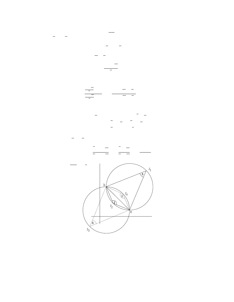
Suppose z lies on the circle
¯
¯
z−a
z−b
¯
¯
and let w be the reflection of z in the
line pz + pz = n. Then by part (ii)
pw + pz = n.
Taking conjugates gives pw + pz = n and hence
z =
n
− pw
p
(a)
Substituting for z in the circle equation, using (a) gives
λ =
¯
¯
¯
¯
¯
n−pw
p
− a
n−pw
p
− b
¯
¯
¯
¯
¯
=
¯
¯
¯
¯
n
− pw − pa
n
− pw − pb
¯
¯
¯
¯
.
(b)
However
n
− pa = |b|
2
− |a|
2
− (b − a)a
= bb
− aa − ba + aa
= b(b
− a) = bp.
Similarly n
− pb = ap. Consequently (b) simplifies to
λ =
¯
¯
¯
¯
bp
− pw
ap
− pw
¯
¯
¯
¯
=
¯
¯
¯
¯
b
− w
a
− w
¯
¯
¯
¯
=
¯
¯
¯
¯
w
− b
w
− a
¯
¯
¯
¯
,
which gives
¯
¯
w−a
w−b
¯
¯
=
1
λ
.
66

11. Let a and b be distinct complex numbers and 0 < α < π.
(i) When z
1
lies on the circular arc shown, it subtends a constant angle
α. This angle is given by Arg (z
1
− a) − Arg (z
1
− b). However
Arg
µ z
1
− a
z
1
− b
= Arg (z
1
− a) − Arg (z
1
− b) + 2kπ
= α + 2kπ.
It follows that k = 0, as 0 < α < π and
−π < Arg θ ≤ π. Hence
Arg
µ z
1
− a
z
1
− b
= α.
Similarly if z
2
lies on the circular arc shown, then
Arg
µ z
2
− a
z
2
− b
=
−γ = −(π − α) = α − π.
Replacing α by π
− α, we deduce that if z
4
lies on the circular arc shown,
then
Arg
µ z
4
− a
z
4
− b
= π
− α,
while if z
3
lies on the circular arc shown, then
Arg
µ z
3
− a
z
3
− b
=
−α.
The straight line through a and b has the equation
z = (1
− t)a + tb,
where t is real. Then 0 < t < 1 describes the segment ab. Also
z
− a
z
− b
=
t
t
− 1
.
Hence
z−a
z−b
is real and negative if z is on the segment a, but is real and positive
if z is on the remaining part of the line, with corresponding values
Arg
µ z
− a
z
− b
= π, 0,
67

respectively.
(ii) Case (a) Suppose z
1
, z
2
and z
3
are not collinear. Then these points
determine a circle. Now z
1
and z
2
partition this circle into two arcs. If z
3
and z
4
lie on the same arc, then
Arg
µ z
3
− z
1
z
3
− z
2
= Arg
µ z
4
− z
1
z
4
− z
2
;
whereas if z
3
and z
4
lie on opposite arcs, then
Arg
µ z
3
− z
1
z
3
− z
2
= α
and
Arg
µ z
4
− z
1
z
4
− z
2
= α
− π.
Hence in both cases
Arg
µ z
3
− z
1
z
3
− z
2
/
z
4
− z
1
z
4
− z
2
≡ Arg
µ z
3
− z
1
z
3
− z
2
− Arg
µ z
4
− z
1
z
4
− z
2
(mod 2π)
≡ 0 or π.
In other words, the cross–ratio
z
3
− z
1
z
3
− z
2
/
z
4
− z
1
z
4
− z
2
is real.
(b) If z
1
, z
2
and z
3
are collinear, then again the cross–ratio is real.
The argument is reversible.
(iii) Assume that A, B, C, D are distinct points such that the cross–ratio
r =
z
3
− z
1
z
3
− z
2
/
z
4
− z
1
z
4
− z
2
is real. Now r cannot be 0 or 1. Then there are three cases:
(i) 0 < r < 1;
(ii) r < 0;
68

(iii) r > 1.
Case (i). Here
|r| + |1 − r| = 1. So
¯
¯
¯
¯
z
4
− z
1
z
4
− z
2
·
z
3
− z
2
z
3
− z
1
¯
¯
¯
¯
+
¯
¯
¯
¯
1
−
µ z
4
− z
1
z
4
− z
2
·
z
3
− z
2
z
3
− z
1
¶¯
¯
¯
¯
= 1.
Multiplying both sides by the denominator
|z
4
− z
2
||z
3
− z
1
| gives after sim-
plification
|z
4
− z
1
||z
3
− z
2
| + |z
2
− z
1
||z
4
− z
3
| = |z
4
− z
2
||z
3
− z
1
|,
or
(a) AD
· BC + AB · CD = BD · AC.
Case (ii). Here 1 +
|r| = |1 − r|. This leads to the equation
(b) BD
· AC + AD · BC+ = AB · CD.
Case (iii). Here 1 +
|1 − r| = |r|. This leads to the equation
(c) BD
· AC + AB · CD = AD · BC.
Conversely if (a), (b) or (c) hold, then we can reverse the argument to deduce
that r is a complex number satisfying one of the equations
|r| + |1 − r| = 1, 1 + |r| = |1 − r|, 1 + |1 − r| = |r|,
from which we deduce that r is real.
69

Section 6.3
1. Let A =
· 4 −3
1
0
¸
. Then A has characteristic equation λ
2
− 4λ + 3 = 0
or (λ
− 3)(λ − 1) = 0. Hence the eigenvalues of A are λ
1
= 3 and λ
2
= 1.
λ
1
= 3. The corresponding eigenvectors satisfy (A
− λ
1
I
2
)X = 0, or
· 1 −3
1
−3
¸
=
· 0
0
¸
,
or equivalently x
− 3y = 0. Hence
· x
y
¸
=
· 3y
y
¸
= y
· 3
1
¸
and we take X
1
=
· 3
1
¸
.
Similarly for λ
2
= 1 we find the eigenvector X
2
=
· 1
1
¸
.
Hence if P = [X
1
|X
2
] =
· 3 1
1 1
¸
, then P is non–singular and
P
−1
AP =
· 3 0
0 1
¸
.
Hence
A = P
· 3 0
0 1
¸
P
−1
and consequently
A
n
= P
· 3
n
0
0
1
n
¸
P
−1
=
· 3 1
1 1
¸ · 3
n
0
0
1
n
¸ 1
2
·
1
−1
−1
3
¸
=
1
2
· 3
n+1
1
3
n
1
¸ ·
1
−1
−1
3
¸
=
1
2
· 3
n+1
− 1 −3
n+1
+ 3
3
n
− 1
−3
n
+ 3
¸
=
3
n
− 1
2
A +
3
− 3
n
2
I
2
.
70

2. Let A =
· 3/5 4/5
2/5 1/5
¸
. Then we find that the eigenvalues are λ
1
= 1 and
λ
2
=
−1/5, with corresponding eigenvectors
X
1
=
· 2
1
¸
and X
2
=
· −1
1
¸
.
Then if P = [X
1
|X
2
], P is non–singular and
P
−1
AP =
· 1
0
0
−1/5
¸
and A = P
· 1
0
0
−1/5
¸
P
−1
.
Hence
A
n
= P
· 1
0
0 (
−1/5)
n
¸
P
−1
→ P
· 1 0
0 0
¸
P
−1
=
· 2 −1
1
1
¸ · 1 0
0 0
¸ 1
3
·
1 1
−1 2
¸
=
1
3
· 2 0
1 0
¸ ·
1 1
−1 2
¸
=
1
3
· 2 2
1 1
¸
=
· 2/3 2/3
1/3 1/3
¸
.
3. The given system of differential equations is equivalent to ˙
X = AX, where
A =
· 3 −2
5
−4
¸
and X =
· x
y
¸
.
The matrix P =
· 2 1
5 1
¸
is a non-singular matrix of eigenvectors corre-
sponding to eigenvalues λ
1
=
−2 and λ
2
= 1. Then
P
−1
AP =
· −2 0
0 1
¸
.
The substitution X = P Y , where Y = [x
1
, y
1
]
t
, gives
˙
Y =
· −2 0
0 1
¸
Y,
71

or equivalently ˙
x
1
=
−2x
1
and ˙
y
1
= y
1
.
Hence x
1
= x
1
(0)e
−2t
and y
1
= y
1
(0)e
t
. To determine x
1
(0) and y
1
(0), we
note that
· x
1
(0)
y
1
(0)
¸
= P
−1
· x(0)
y(0)
¸
=
−
1
3
·
1
−1
−5
2
¸ · 13
22
¸
=
· 3
7
¸
.
Hence x
1
= 3e
−2t
and y
1
= 7e
t
. Consequently
x = 2x
1
+ y
1
= 6e
−2t
+ 7e
t
and y = 5x
1
+ y
1
= 15e
−2t
+ 7e
t
.
4. Introducing the vector X
n
=
· x
n
y
n
¸
, the system of recurrence relations
x
n+1
= 3x
n
− y
n
y
n+1
=
−x
n
+ 3y
n
,
becomes X
n+1
= AX
n
, where A =
·
3
−1
−1
3
¸
. Hence X
n
= A
n
X
0
, where
X
0
=
· 1
2
¸
.
To find A
n
we can use the eigenvalue method. We get
A
n
=
1
2
· 2
n
+ 4
n
2
n
− 4
n
2
n
− 4
n
2
n
+ 4
n
¸
.
Hence
X
n
=
1
2
· 2
n
+ 4
n
2
n
− 4
n
2
n
− 4
n
2
n
+ 4
n
¸ · 1
2
¸
=
1
2
· 2
n
+ 4
n
+ 2(2
n
− 4
n
)
2
n
− 4
n
+ 2(2
n
+ 4
n
)
¸
=
1
2
· 3 × 2
n
− 4
n
3
× 2
n
+ 4
n
¸
=
· (3 × 2
n
− 4
n
)/2
(3
× 2
n
+ 4
n
)/2
¸
.
Hence x
n
=
1
2
(3
× 2
n
− 4
n
) and y
n
=
1
2
(3
× 2
n
+ 4
n
).
5. Let A =
· a b
c d
¸
be a real or complex matrix with distinct eigenvalues
λ
1
, λ
2
and corresponding eigenvectors X
1
, X
2
. Also let P = [X
1
|X
2
].
72

(a) The system of recurrence relations
x
n+1
= ax
n
+ by
n
y
n+1
= cx
n
+ dy
n
has the solution
· x
n
y
n
¸
= A
n
· x
0
y
0
¸
=
µ
P
· λ
1
0
0
λ
2
¸
P
−1
n
· x
0
y
0
¸
= P
· λ
n
1
0
0
λ
n
2
¸
P
−1
· x
0
y
0
¸
= [X
1
|X
2
]
· λ
n
1
0
0
λ
n
2
¸ · α
β
¸
= [X
1
|X
2
]
· λ
n
1
α
λ
n
2
β
¸
= λ
n
1
αX
1
+ λ
n
2
βX
2
,
where
· α
β
¸
= P
−1
· x
0
y
0
¸
.
(b) In matrix form, the system is ˙
X = AX, where X =
· x
y
¸
. We substitute
X = P Y , where Y = [x
1
, y
1
]
t
. Then
˙
X = P ˙
Y = AX = A(P Y ),
so
˙
Y = (P
−1
AP )Y =
· λ
1
0
0
λ
2
¸ · x
1
y
1
¸
.
Hence ˙
x
1
= λ
1
x
1
and ˙
y
1
= λ
2
y
1
. Then
x
1
= x
1
(0)e
λ
1
t
and y
1
= y
1
(0)e
λ
2
t
.
But
· x(0)
y(0)
¸
= P
· x
1
(0)
y
1
(0)
¸
,
so
· x
1
(0)
y
1
(0)
¸
= P
−1
· x(0)
y(0)
¸
=
· α
β
¸
.
73

Consequently x
1
(0) = α and y
1
(0) = β and
· x
y
¸
= P
· x
1
y
1
¸
= [X
1
|X
2
]
· αe
λ
1
t
βe
λ
2
t
¸
= αe
λ
1
t
X
1
+ βe
λ
2
t
X
2
.
6. Let A =
· a b
c d
¸
be a real matrix with non–real eigenvalues λ = a + ib
and λ = a
−ib, with corresponding eigenvectors X = U +iV and X = U −iV ,
where U and V are real vectors. Also let P be the real matrix defined by
P = [U
|V ]. Finally let a + ib = re
iθ
, where r > 0 and θ is real.
(a) As X is an eigenvector corresponding to the eigenvalue λ, we have AX =
λX and hence
A(U + iV ) = (a + ib)(U + iV )
AU + iAV
= aU
− bV + i(bU + aV ).
Equating real and imaginary parts then gives
AU = aU
− bV
AV
= bU + aV.
(b)
AP = A[U
|V ] = [AU|AV ] = [aU−bV |bU+aV ] = [U|V ]
·
a b
−b a
¸
= P
·
a b
−b a
¸
.
Hence, as P can be shown to be non–singular,
P
−1
AP =
·
a b
−b a
¸
.
(The fact that P is non–singular is easily proved by showing the columns of
P are linearly independent: Assume xU + yV = 0, where x and y are real.
Then we find
(x + iy)(U
− iV ) + (x − iy)(U + iV ) = 0.
74

Consequently x+iy = 0 as U
−iV and U +iV are eigenvectors corresponding
to distinct eigenvalues a
− ib and a + ib and are hence linearly independent.
Hence x = 0 and y = 0.)
(c) The system of recurrence relations
x
n+1
= ax
n
+ by
n
y
n+1
= cx
n
+ dy
n
has solution
· x
n
y
n
¸
= A
n
· x
0
y
0
¸
= P
·
a b
−b a
¸
n
P
−1
· x
0
y
0
¸
= P
·
r cos θ
r sin θ
−r sin θ r cos θ
¸
n
· α
β
¸
= P r
n
·
cos θ
sin θ
− sin θ cos θ
¸
n
· α
β
¸
= r
n
[U
|V ]
·
cos nθ
sin nθ
− sin nθ cos nθ
¸ · α
β
¸
= r
n
[U
|V ]
·
α cos nθ + β sin nθ
−α sin nθ + β cos nθ
¸
= r
n
{(α cos nθ + β sin nθ)U + (−α sin nθ + β cos nθ)V }
= r
n
{(cos nθ)(αU + βV ) + (sin nθ)(βU − αV )} .
(d) The system of differential equations
dx
dt
= ax + by
dy
dt
= cx + dy
is attacked using the substitution X = P Y , where Y = [x
1
, y
1
]
t
. Then
˙
Y = (P
−1
AP )Y,
so
·
˙
x
1
˙
y
1
¸
=
·
a b
−b a
¸ · x
1
y
1
¸
.
75

Equating components gives
˙
x
1
= ax
1
+ by
1
˙
y
1
=
−bx
1
+ ay
1
.
Now let z = x
1
+ iy
1
. Then
˙z = ˙
x
1
+ i ˙
y
1
= (ax
1
+ by
1
) + i(
−bx
1
+ ay
1
)
= (a
− ib)(x
1
+ iy
1
) = (a
− ib)z.
Hence
z = z(0)e
(a−ib)t
x
1
+ iy
1
= (x
1
(0) + iy
1
(0))e
at
(cos bt
− i sin bt).
Equating real and imaginary parts gives
x
1
= e
at
{x
1
(0) cos bt + y
1
(0) sin bt
}
y
1
= e
at
{y
1
(0) cos bt
− x
1
(0) sin bt
} .
Now if we define α and β by
· α
β
¸
= P
−1
· x(0)
y(0)
¸
,
we see that α = x
1
(0) and β = y
1
(0). Then
· x
y
¸
= P
· x
1
y
1
¸
= [U
|V ]
· e
at
(α cos bt + β sin bt)
e
at
(β cos bt
− α sin bt)
¸
= e
at
{(α cos bt + β sin bt)U + (β cos bt − α sin bt)V }
= e
at
{cos bt(αU + βV ) + sin bt(βU − αV )}.
7. (The case of repeated eigenvalues.) Let A =
· a b
c d
¸
and suppose that
the characteristic polynomial of A, λ
2
− (a + d)λ + (ad − bc), has a repeated
root α. Also assume that A
6= αI
2
.
76

(i)
λ
2
− (a + d)λ + (ad − bc) = (λ − α)
2
= λ
2
− 2αλ + α
2
.
Hence a + d = 2α and ad
− bc = α
2
and
(a + d)
2
= 4(ad
− bc),
a
2
+ 2ad + d
2
= 4ad
− 4bc,
a
2
− 2ad + d
2
+ 4bc = 0,
(a
− d)
2
+ 4bc = 0.
(ii) Let B
− A − αI
2
. Then
B
2
= (A
− αI
2
)
2
= A
2
− 2αA + α
2
I
2
= A
2
− (a + d)A + (ad − bc)I
2
,
But by problem 3, chapter 2.4, A
2
− (a + d)A + (ad − bc)I
2
= 0, so
B
2
= 0.
(iii) Now suppose that B
6= 0. Then BE
1
6= 0 or BE
2
6= 0, as BE
i
is the
i–th column of B. Hence BX
2
6= 0, where X
2
= E
1
or X
2
= E
2
.
(iv) Let X
1
= BX
2
and P = [X
1
|X
2
]. We prove P is non–singular by
demonstrating that X
1
and X
2
are linearly independent.
Assume xX
1
+ yX
2
= 0. Then
xBX
2
+ yX
2
= 0
B(xBX
2
+ yX
2
) = B0 = 0
xB
2
X
2
+ yBX
2
= 0
x0X
2
+ yBX
2
= 0
yBX
2
= 0.
Hence y = 0 as BX
2
6= 0. Hence xBX
2
= 0 and so x = 0.
Finally, BX
1
= B(BX
2
) = B
2
X
2
= 0, so (A
− αI
2
)X
1
= 0 and
AX
1
= αX
1
.
(2)
77

Also
X
1
= BX
2
= (A
− αI
2
)X
2
= AX
2
− αX
2
.
Hence
AX
2
= X
1
+ αX
2
.
(3)
Then, using (2) and (3), we have
AP = A[X
1
|X
2
] = [AX
1
|AX
2
]
= [αX
1
|X
1
+ αX
2
]
= [X
1
|X
2
]
· α 1
0 α
¸
.
Hence
AP = P
· α 1
0 α
¸
and hence
P
−1
AP =
· α 1
0 α
¸
.
8. The system of differential equations is equivalent to the single matrix
equation ˙
X = AX, where A =
· 4 −1
4
8
¸
.
The characteristic polynomial of A is λ
2
− 12λ + 36 = (λ − 6)
2
, so we can
use the previous question with α = 6. Let
B = A
− 6I
2
=
· −2 −1
4
2
¸
.
Then BX
2
=
· −2
4
¸
6=
· 0
0
¸
, if X
2
=
· 1
0
¸
. Also let X
1
= BX
2
. Then if
P = [X
1
|X
2
], we have
P
−1
AP =
· 6 1
0 6
¸
.
Now make the change of variables X = P Y , where Y =
· x
1
y
1
¸
. Then
˙
Y = (P
−1
AP )Y =
· 6 1
0 6
¸
Y,
78

or equivalently ˙
x
1
= 6x
1
+ y
1
and ˙
y
1
= 6y
1
.
Solving for y
1
gives y
1
= y
1
(0)e
6t
. Consequently
˙
x
1
= 6x
1
+ y
1
(0)e
6t
.
Multiplying both side of this equation by e
−6t
gives
d
dt
(e
−6t
x
1
) = e
−6t
˙
x
1
− 6e
−6t
x
1
= y
1
(0)
e
−6t
x
1
= y
1
(0)t + c,
where c is a constant. Substituting t = 0 gives c = x
1
(0). Hence
e
−6t
x
1
= y
1
(0)t + x
1
(0)
and hence
x
1
= e
6t
(y
1
(0)t + x
1
(0)).
However, since we are assuming x(0) = 1 = y(0), we have
· x
1
(0)
y
1
(0)
¸
= P
−1
· x(0)
y(0)
¸
=
1
−4
·
0
−1
−4 −2
¸ · 1
1
¸
=
1
−4
· −1
−6
¸
=
· 1/4
3/2
¸
.
Hence x
1
= e
6t
(
3
2
t +
1
4
) and y
1
=
3
2
e
6t
.
Finally, solving for x and y,
· x
y
¸
=
· −2 1
4 0
¸ · x
1
y
1
¸
=
· −2 1
4 0
¸
e
6t
(
3
2
t +
1
4
)
3
2
e
6t
=
(
−2)e
6t
(
3
2
t +
1
4
) +
3
2
e
6t
4e
6t
(
3
2
t +
1
4
)
=
· e
6t
(1
− 3t)
e
6t
(6t + 1)
¸
.
Hence x = e
6t
(1
− 3t) and y = e
6t
(6t + 1).
79

9. Let
A =
1/2 1/2
0
1/4 1/4 1/2
1/4 1/4 1/2
.
(a) We first determine the characteristic polynomial ch
A
(λ).
ch
A
(λ) = det (λI
3
− A) =
¯
¯
¯
¯
¯
¯
λ
− 1/2
−1/2
0
1/4 λ
− 1/4
−1/2
−1/4
−1/4 λ − 1/2
¯
¯
¯
¯
¯
¯
=
µ
λ
−
1
2
¶ ¯
¯
¯
¯
λ
− 1/4
−1/2
−1/4 λ − 1/2
¯
¯
¯
¯
+
1
2
¯
¯
¯
¯
1/4
−1/2
−1/4 λ − 1/2
¯
¯
¯
¯
=
µ
λ
−
1
2
¶ ½µ
λ
−
1
4
¶ µ
λ
−
1
2
−
1
8
¾
+
1
2
½
−1
4
µ
λ
−
1
2
−
1
8
¾
=
µ
λ
−
1
2
¶ µ
λ
2
−
3λ
4
−
λ
8
= λ
½µ
λ
−
1
2
¶ µ
λ
−
3
4
−
1
8
¾
= λ
µ
λ
2
−
5λ
4
+
1
4
= λ(λ
− 1)
µ
λ
−
1
4
.
(b) Hence the characteristic polynomial has no repeated roots and we can
use Theorem 6.2.2 to find a non–singular matrix P such that
P
−1
AP = diag(1, 0,
1
4
).
We take P = [X
1
|X
2
|X
3
], where X
1
, X
2
, X
3
are eigenvectors corresponding
to the respective eigenvalues 1, 0,
1
4
.
Finding X
1
: We have to solve (A
− I
3
)X = 0. we have
A
− I
3
=
−1/2
1/2
0
1/4
−3/4
1/2
1/4
1/4
−1/2
→
1 0
−1
0 1
−1
0 0
0
.
Hence the eigenspace consists of vectors X = [x, y, z]
t
satisfying x = z and
80

y = z, with z arbitrary. Hence
X =
z
z
z
= z
1
1
1
and we can take X
1
= [1, 1, 1]
t
.
Finding X
2
: We solve AX = 0. We have
A =
1/2 1/2
0
1/4 1/4 1/2
1/4 1/4 1/2
→
1 1 0
0 0 1
0 0 0
.
Hence the eigenspace consists of vectors X = [x, y, z]
t
satisfying x =
−y and
z = 0, with y arbitrary. Hence
X =
−y
y
0
= y
−1
1
0
and we can take X
2
= [
−1, 1, 0]
t
.
Finding X
3
: We solve (A
−
1
4
I
3
)X = 0. We have
A
−
1
4
I
3
=
1/4 1/2
0
1/4
0
1/2
1/4 1/4 1/4
→
1 0
2
0 1
−1
0 0
0
.
Hence the eigenspace consists of vectors X = [x, y, z]
t
satisfying x =
−2z
and y = z, with z arbitrary. Hence
X =
−2z
z
0
= z
−2
1
0
and we can take X
3
= [
−2, 1, 1]
t
.
Hence we can take P =
1
−1 −2
1
1
1
1
0
1
.
(c) A = P diag(1, 0,
1
4
)P
−1
so A
n
= P diag(1, 0,
1
4
n
)P
−1
.
81

Hence
A
n
=
1
−1 −2
1
1
1
1
0
1
1 0
0
0 0
0
0 0
1
4
n
1
3
1
1
1
0
3
−3
−1 −1
2
=
1
3
1 0
−
2
4
n
1 0
1
4
n
1 0
1
4
n
1
1
1
0
3
−3
−1 −1
2
=
1
3
1 +
2
4
n
1 +
2
4
n
1
−
4
4
n
1
−
1
4
n
1
−
1
4
n
1 +
2
4
n
1
−
1
4
n
1
−
1
4
n
1 +
2
4
n
=
1
3
1 1 1
1 1 1
1 1 1
+
1
3
· 4
n
2
2
−4
−1 −1
2
−1 −1
2
.
10. Let
A =
5
2
−2
2
5
−2
−2 −2
5
.
(a) We first determine the characteristic polynomial ch
A
(λ).
ch
A
(λ) =
¯
¯
¯
¯
¯
¯
λ
− 5
−2
2
−2
λ
− 5
2
2
2
λ
− 5
R
3
→ R
3
+ R
2
=
¯
¯
¯
¯
¯
¯
λ
− 5
−2
2
−2
λ
− 5
2
0
λ
− 3 λ − 3
¯
¯
¯
¯
¯
¯
= (λ
− 3)
¯
¯
¯
¯
¯
¯
λ
− 5
−2
2
−2
λ
− 5 2
0
1
1
¯
¯
¯
¯
¯
¯
C
3
→ C
3
− C
2
= (λ
− 3)
¯
¯
¯
¯
¯
¯
λ
− 5
−2
4
−2
λ
− 5 −λ + 7
0
1
0
¯
¯
¯
¯
¯
¯
=
−(λ − 3)
¯
¯
¯
¯
λ
− 5
4
−2
−λ + 7
¯
¯
¯
¯
=
−(λ − 3) {(λ − 5)(−λ + 7) + 8}
=
−(λ − 3)(−λ
2
+ 5λ + 7λ
− 35 + 8)
=
−(λ − 3)(−λ
2
+ 12λ
− 27)
82

=
−(λ − 3)(−1)(λ − 3)(λ − 9)
= (λ
− 3)
2
(λ
− 9).
We have to find bases for each of the eigenspaces N (A
−9I
3
) and N (A
−3I
3
).
First we solve (A
− 3I
3
)X = 0. We have
A
− 3I
3
=
2
2
−2
2
2
−2
−2 −2
2
→
1 1
−1
0 0
0
0 0
0
.
Hence the eigenspace consists of vectors X = [x, y, z]
t
satisfying x =
−y + z,
with y and z arbitrary. Hence
X =
−y + z
y
z
= y
−1
1
0
+ z
1
0
1
,
so X
1
= [
−1, 1, 0]
t
and X
2
= [1, 0, 1]
t
form a basis for the eigenspace corre-
sponding to the eigenvalue 3.
Next we solve (A
− 9I
3
)X = 0. We have
A
− 9I
3
=
−4
2
−2
2
−4 −2
−2 −2 −4
→
1 0 1
0 1 1
0 0 0
.
Hence the eigenspace consists of vectors X = [x, y, z]
t
satisfying x =
−z and
y =
−z, with z arbitrary. Hence
X =
−z
−z
z
= z
−1
−1
1
and we can take X
3
= [
−1, −1, 1]
t
as a basis for the eigenspace corresponding
to the eigenvalue 9.
Then Theorem 6.2.3 assures us that P = [X
1
|X
2
|X
3
] is non–singular and
P
−1
AP =
3 0 0
0 3 0
0 0 9
.
83
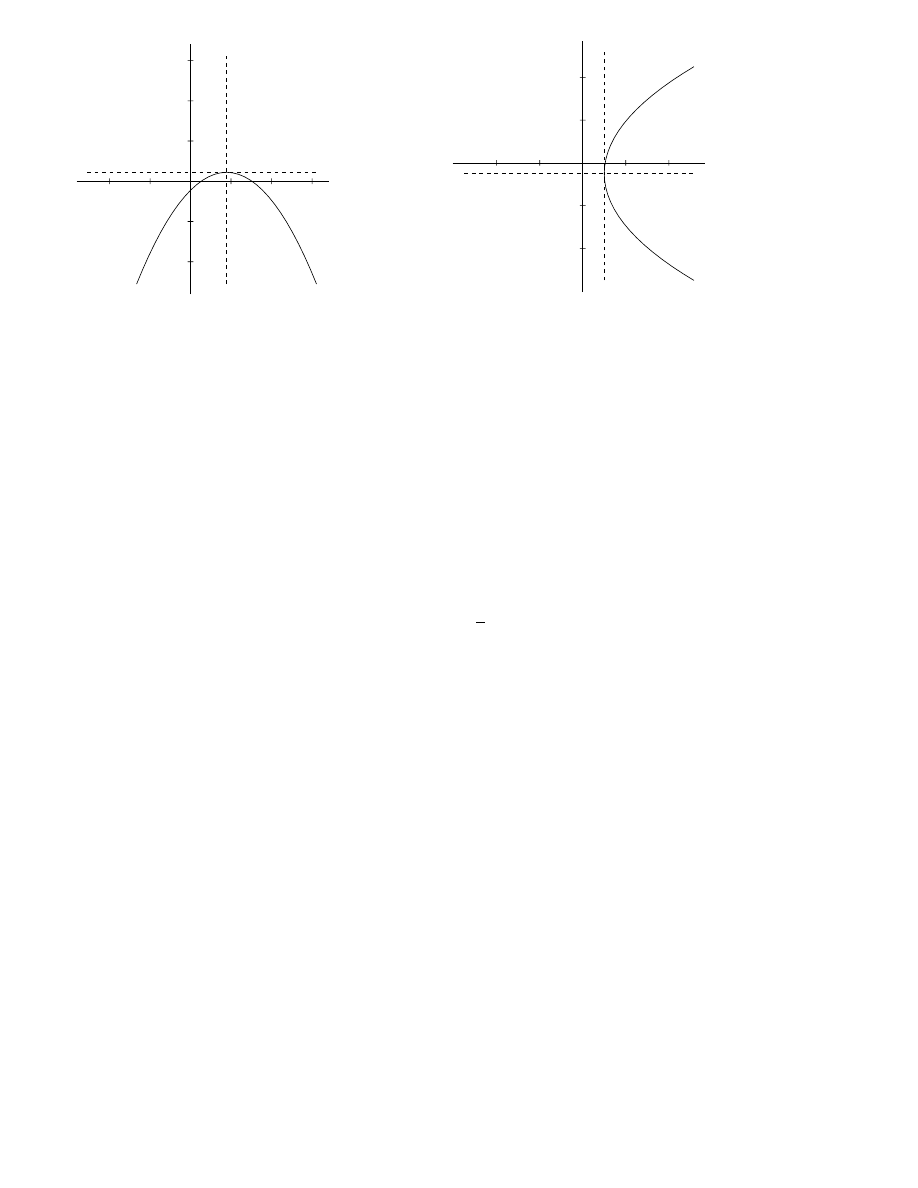
x
1
y
1
4.5
9
13.5
-4.5
-9
4.5
9
13.5
-4.5
-9
x
y
x
1
y
1
4
8
-4
-8
4
8
-4
-8
x
y
Figure 1: (a): x
2
− 8x + 8y + 8 = 0;
(b): y
2
− 12x + 2y + 25 = 0
Section 7.3
1. (i) x
2
−8x+8y+8 = (x−4)
2
+8(y
−1). So the equation x
2
−8x+8y+8 = 0
becomes
x
2
1
+ 8y
1
= 0
(1)
if we make a translation of axes x
− 4 = x
1
, y
− 1 = y
1
.
However equation (1) can be written as a standard form
y
1
=
−
1
8
x
2
1
,
which represents a parabola with vertex at (4, 1). (See Figure 1(a).)
(ii) y
2
− 12x + 2y + 25 = (y + 1)
2
− 12(x − 2). Hence y
2
− 12x + 2y + 25 = 0
becomes
y
2
1
− 12x
1
= 0
(2)
if we make a translation of axes x
− 2 = x
1
, y + 1 = y
1
.
However equation (2) can be written as a standard form
y
2
1
= 12x
1
,
which represents a parabola with vertex at (2,
−1). (See Figure 1(b).)
2. 4xy
− 3y
2
= X
t
AX, where A =
· 0
2
2
−3
¸
and X =
· x
y
¸
. The eigenval-
ues of A are the roots of λ
2
+ 3λ
− 4 = 0, namely λ
1
=
−4 and λ
2
= 1.
84

The eigenvectors corresponding to an eigenvalue λ are the non–zero vec-
tors [x, y]
t
satisfying
· 0 − λ
2
2
−3 − λ
¸ · x
y
¸
=
· 0
0
¸
.
λ
1
=
−4 gives equations
4x + 2y = 0
2x + y = 0
which has the solution y =
−2x. Hence
· x
y
¸
=
·
x
−2x
¸
= x
·
1
−2
¸
.
A corresponding unit eigenvector is [1/
√
5,
−2/
√
5]
t
.
λ
2
= 1 gives equations
−x + 2y = 0
2x
− 4y = 0
which has the solution x = 2y. Hence
· x
y
¸
=
· 2y
y
¸
= y
· 2
1
¸
.
A corresponding unit eigenvector is [2/
√
5, 1/
√
5]
t
.
Hence if
P =
"
1
√
5
2
√
5
−2
√
5
1
√
5
#
,
then P is an orthogonal matrix. Also as det P = 1, P is a proper orthogonal
matrix and the equation
· x
y
¸
= P
· x
1
y
1
¸
represents a rotation to new x
1
, y
1
axes whose positive directions are given
by the respective columns of P . Also
P
t
AP =
· −4 0
0 1
¸
.
85

Then X
t
AX =
−4x
2
1
+ y
2
1
and the original equation 4xy
− 3y
2
= 8 becomes
−4x
2
1
+ y
2
1
= 8, or the standard form
−x
2
1
2
+
y
2
1
8
= 1,
which represents an hyperbola.
The asymptotes assist in drawing the curve. They are given by the equa-
tions
−x
2
1
2
+
y
2
1
8
= 0,
or y
1
=
±2x
1
.
Now
· x
1
y
1
¸
= P
t
· x
y
¸
=
"
1
√
5
−2
√
5
2
√
5
1
√
5
#
· x
y
¸
,
so
x
1
=
x
− 2y
√
5
,
y
1
=
2x + y
√
5
.
Hence the asymptotes are
2x + y
√
5
=
±2
µ x
− 2y
√
5
,
which reduces to y = 0 and y = 4x/3. (See Figure 2(a).)
3. 8x
2
− 4xy + 5y
2
= X
t
AX, where A =
·
8
−2
−2
5
¸
and X =
· x
y
¸
. The
eigenvalues of A are the roots of λ
2
− 13λ + 36 = 0, namely λ
1
= 4 and
λ
2
= 9. Corresponding unit eigenvectors turn out to be [1/
√
5, 2/
√
5]
t
and
[
−2/
√
5, 1/
√
5]
t
. Hence if
P =
"
1
√
5
−2
√
5
2
√
5
1
√
5
#
,
then P is an orthogonal matrix. Also as det P = 1, P is a proper orthogonal
matrix and the equation
· x
y
¸
= P
· x
1
y
1
¸
represents a rotation to new x
1
, y
1
axes whose positive directions are given
by the respective columns of P . Also
P
t
AP =
· 4 0
0 9
¸
.
86
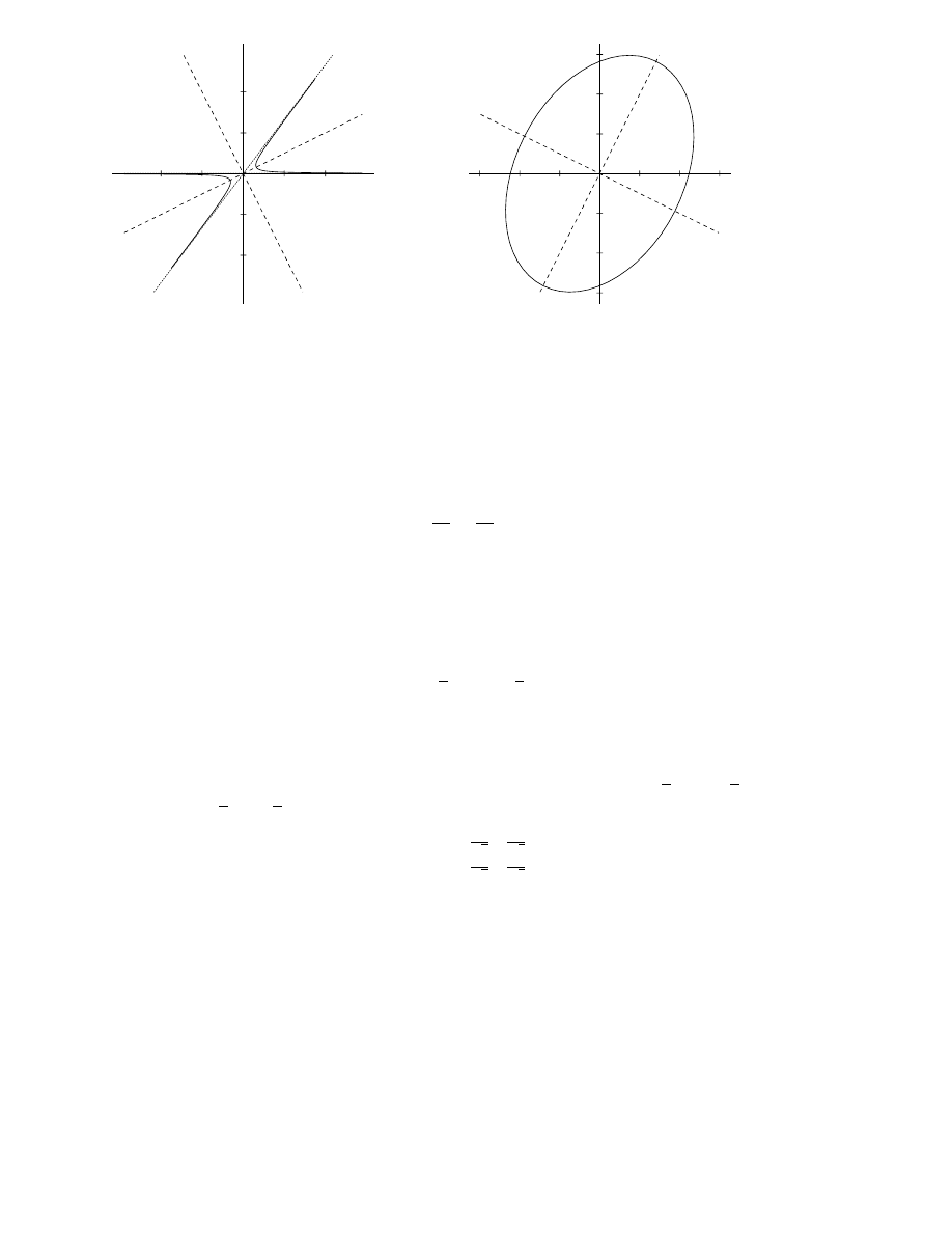
x
2
y
2
8
16
-8
-16
8
16
-8
-16
x
y
x
2
y
2
0.95
1.9
2.85
-0.95
-1.9
-2.85
0.95
1.9
2.85
-0.95
-1.9
-2.85
x
y
Figure 2: (a): 4xy
− 3y
2
= 8;
(b): 8x
2
− 4xy + 5y
2
= 36
Then X
t
AX = 4x
2
1
+ 9y
2
1
and the original equation 8x
2
− 4xy + 5y
2
= 36
becomes 4x
2
1
+ 9y
2
1
= 36, or the standard form
x
2
1
9
+
y
2
1
4
= 1,
which represents an ellipse as in Figure 2(b).
The axes of symmetry turn out to be y = 2x and x =
−2y.
4. We give the sketch only for parts (i), (iii) and (iv). We give the working
for (ii) only. See Figures 3(a) and 4(a) and 4(b), respectively.
(ii) We have to investigate the equation
5x
2
− 4xy + 8y
2
+ 4
√
5x
− 16
√
5y + 4 = 0.
(3)
Here 5x
2
− 4xy + 8y
2
= X
t
AX, where A =
·
5
−2
−2
8
¸
and X =
· x
y
¸
.
The eigenvalues of A are the roots of λ
2
− 13λ + 36 = 0, namely λ
1
= 9 and
λ
2
= 4. Corresponding unit eigenvectors turn out to be [1/
√
5,
−2/
√
5]
t
and
[2/
√
5, 1/
√
5]
t
. Hence if
P =
"
1
√
5
2
√
5
−2
√
5
1
√
5
#
,
then P is an orthogonal matrix. Also as det P = 1, P is a proper orthogonal
matrix and the equation
· x
y
¸
= P
· x
1
y
1
¸
87
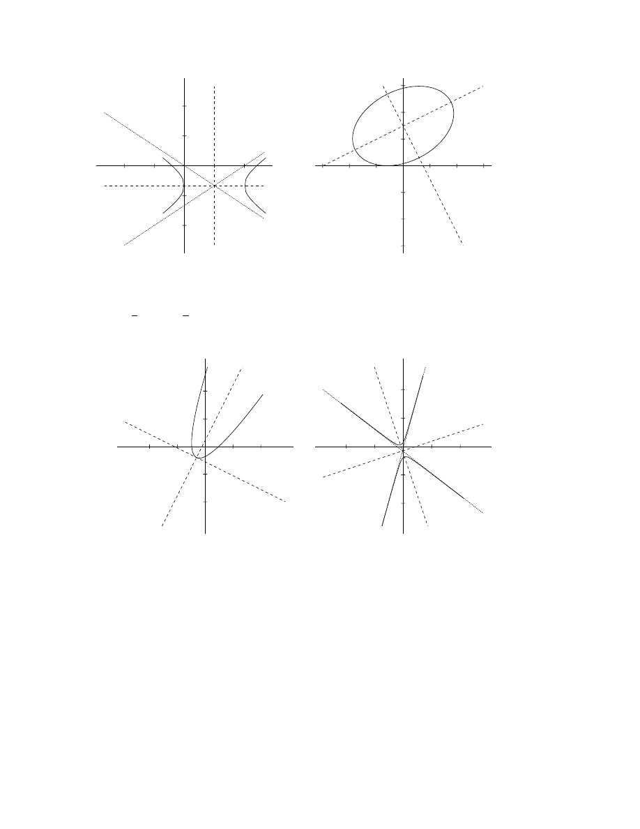
x
1
y
1
3
6
-3
-6
3
6
-3
-6
x
y
x
2
y
2
1.5
3
4.5
-1.5
-3
-4.5
1.5
3
4.5
-1.5
-3
-4.5
x
y
Figure 3: (a): 4x
2
− 9y
2
− 24x − 36y − 36 = 0;
(b): 5x
2
− 4xy + 8y
2
+
√
5x
− 16
√
5y + 4 = 0
x
2
y
2
4.5
9
-4.5
-9
4.5
9
-4.5
-9
x
y
x
2
y
2
4.5
9
-4.5
-9
4.5
9
-4.5
-9
x
y
Figure 4: (a): 4x
2
+ y
2
− 4xy − 10y − 19 = 0;
(b): 77x
2
+ 78xy
− 27y
2
+
70x
− 30y + 29 = 0
88

represents a rotation to new x
1
, y
1
axes whose positive directions are given
by the respective columns of P . Also
P
t
AP =
· 9 0
0 4
¸
.
Moreover
5x
2
− 4xy + 8y
2
= 9x
2
1
+ 4y
2
1
.
To get the coefficients of x
1
and y
1
in the transformed form of equation (3),
we have to use the rotation equations
x =
1
√
5
(x
1
+ 2y
1
),
y =
1
√
5
(
−2x
1
+ y
1
).
Then equation (3) transforms to
9x
2
1
+ 4y
2
1
+ 36x
1
− 8y
1
+ 4 = 0,
or, on completing the square,
9(x
1
+ 2)
2
+ 4(y
1
− 1)
2
= 36,
or in standard form
x
2
2
4
+
y
2
2
9
= 1,
where x
2
= x
1
+ 2 and y
2
= y
1
− 1. Thus we have an ellipse, centre (x
2
, y
2
) =
(0, 0), or (x
1
, y
1
) = (
−2, 1), or (x, y) = (0,
√
5).
The axes of symmetry are given by x
2
= 0 and y
2
= 0, or x
1
+ 2 = 0 and
y
1
− 1 = 0, or
1
√
5
(x
− 2y) + 2 = 0 and
1
√
5
(2x + y)
− 1 = 0,
which reduce to x
− 2y + 2
√
5 = 0 and 2x + y
−
√
5 = 0. See Figure 3(b).
5. (i) Consider the equation
2x
2
+ y
2
+ 3xy
− 5x − 4y + 3 = 0.
(4)
∆ =
¯
¯
¯
¯
¯
¯
2 3/2
−5/2
3/2
1
−2
−5/2 −2
3
¯
¯
¯
¯
¯
¯
= 8
¯
¯
¯
¯
¯
¯
4
3
−5
3
2
−4
−5 −4
6
¯
¯
¯
¯
¯
¯
= 8
¯
¯
¯
¯
¯
¯
1
1
−1
3
2
−4
−2 −2
2
¯
¯
¯
¯
¯
¯
= 0.
89

Let x = x
1
+ α, y = y
1
+ β and substitute in equation (4) to get
2(x
1
+ α)
2
+ (y
1
+ β)
2
+ 3(x
1
+ α)(y
1
+ β)
− 5(x
1
+ α)
− 4(y
1
+ β) + 3 = 0 (5).
Then equating the coefficients of x
1
and y
1
to 0 gives
4α + 3β
− 5 = 0
3α + 2β
− 4 = 0,
which has the unique solution α = 2, β =
−1. Then equation (5) simplifies
to
2x
2
1
+ y
2
1
+ 3x
1
y
1
= 0 = (2x
1
+ y
1
)(x
1
+ y
1
).
So relative to the x
1
, y
1
coordinates, equation (4) describes two lines: 2x
1
+
y
1
= 0 and x
1
+ y
1
= 0. In terms of the original x, y coordinates, these lines
become 2(x
− 2) + (y + 1) = 0 and (x − 2) + (y + 1) = 0, i.e. 2x + y − 3 = 0
and x + y
− 1 = 0, which intersect in the point
(x, y) = (α, β) = (2,
−1).
(ii) Consider the equation
9x
2
+ y
2
− 6xy + 6x − 2y + 1 = 0. (6)
Here
∆ =
¯
¯
¯
¯
¯
¯
9
−3
3
3
1
−1
3
−1
1
¯
¯
¯
¯
¯
¯
= 0,
as column 3 =
− column 2.
Let x = x
1
+ α, y = y
1
+ β and substitute in equation (6) to get
9(x
1
+ α)
2
+ (y
1
+ β)
2
− 6(x
1
+ α)(y
1
+ β) + 6(x
1
+ α)
− 2(y
1
+ β) + 1 = 0.
Then equating the coefficients of x
1
and y
1
to 0 gives
18α
− 6β + 6 = 0
−6α + 2β − 2 = 0,
or equivalently
−3α + β − 1 = 0. Take α = 0 and β = 1. Then equation (6)
simplifies to
9x
2
1
+ y
2
1
− 6x
1
y
1
= 0 = (3x
1
− y
1
)
2
.
(7)
90

In terms of x, y coordinates, equation (7) becomes
(3x
− (y − 1))
2
= 0, or 3x
− y + 1 = 0.
(iii) Consider the equation
x
2
+ 4xy + 4y
2
− x − 2y − 2 = 0.
(8)
Arguing as in the previous examples, we find that any translation
x = x
1
+ α,
y = y
1
+ β
where 2α + 4β
− 1 = 0 has the property that the coefficients of x
1
and y
1
will
be zero in the transformed version of equation (8). Take β = 0 and α = 1/2.
Then (8) reduces to
x
2
1
+ 4x
1
y
1
+ 4y
2
1
−
9
4
= 0,
or (x
1
+ 2y
1
)
2
= 3/2. Hence x
1
+ 2y
1
=
±3/2, with corresponding equations
x + 2y = 2 and x + 2y =
−1.
91

Section 8.8
1. The given line has equations
x = 3 + t(13
− 3) = 3 + 10t,
y =
−2 + t(3 + 2) = −2 + 5t,
z = 7 + t(
−8 − 7) = 7 − 15t.
The line meets the plane y = 0 in the point (x, 0, z), where 0 =
−2 + 5t, or
t = 2/5. The corresponding values for x and z are 7 and 1, respectively.
2. E =
1
2
(B + C), F = (1
− t)A + tE, where
t =
AF
AE
=
AF
AF + F E
=
AF/F E
(AF/F E) + 1
=
2
3
.
Hence
F
=
1
3
A
+
2
3
µ 1
2
(B + C)
=
1
3
A
+
1
3
(B + C)
=
1
3
(A + B + C).
3. Let A = (2, 1, 4), B = (1,
−1, 2), C = (3, 3, 6). Then we prove
-
AC=
t
-
AB for some real t. We have
-
AC=
1
2
2
,
-
AB=
−1
−2
−2
.
Hence
-
AC= (
−1)
-
AB and consequently C is on the line AB. In fact A is
between C and B, with AC = AB.
4. The points P on the line AB which satisfy AP =
2
5
P B are given by
P
= A + t
-
AB, where
|t/(1 − t)| = 2/5. Hence t/(1 − t) = ±2/5.
The equation t/(1
− t) = 2/5 gives t = 2/7 and hence
P
=
2
3
−1
+
2
7
1
4
5
=
16/7
29/7
3/7
.
92

Hence P = (16/7, 29/7, 3/7).
The equation t/(1
− t) = −2/5 gives t = −2/3 and hence
P
=
2
3
−1
−
2
3
1
4
5
=
4/3
1/3
−13/3
.
Hence P = (4/3, 1/3,
−13/3).
5. An equation for
M is P = A + t
-
BC, which reduces to
x = 1 + 6t
y = 2
− 3t
z = 3 + 7t.
An equation for
N is Q = E + s
-
EF , which reduces to
x = 1 + 9s
y =
−1
z = 8 + 3s.
To find if and where
M and N intersect, we set P = Q and attempt to solve
for s and t. We find the unique solution t = 1, s = 2/3, proving that the
lines meet in the point
(x, y, z) = (1 + 6, 2
− 3, 3 + 7) = (7, −1, 10).
6. Let A = (3, 5, 6), B = (
−2, 7, 9), C = (2, 1, 7). Then
(i)
cos ∠ABC = (
-
BA
·
-
BC)/(BA
· BC),
where
-
BA= [
−1, −2, −3]
t
and
-
BC= [4,
−6, −2]
t
. Hence
cos ∠ABC =
−4 + 12 + 6
√
14
√
56
=
14
√
14
√
56
=
1
2
.
Hence ∠ABC = π/3 radians or 60
◦
.
93

(ii)
cos ∠BAC = (
-
AB
·
-
AC)/(AB
· AC),
where
-
AB= [1, 2, 3]
t
and
-
AC= [5,
−4, 1]
t
. Hence
cos ∠BAC =
5
− 8 + 3
√
14
√
42
= 0.
Hence ∠ABC = π/2 radians or 90
◦
.
(iii)
cos ∠ACB = (
-
CA
·
-
CB)/(CA
· CB),
where
-
CA= [
−5, 4, −1]
t
and
-
CB= [
−4, 6, 2]
t
. Hence
cos ∠ACB =
20 + 24
− 2
√
42
√
56
=
42
√
42
√
56
=
√
42
√
56
=
√
3
2
.
Hence ∠ACB = π/6 radians or 30
◦
.
7. By Theorem 8.5.2, the closest point P on the line AB to the origin O is
given by P = A + t
-
AB, where
t =
-
AO
·
-
AB
AB
2
=
−A·
-
AB
AB
2
.
Now
A
·
-
AB=
−2
1
3
·
3
1
1
=
−2.
Hence t = 2/11 and
P
=
−2
1
3
+
2
11
3
1
1
=
−16/11
13/11
35/11
and P = (
−16/11, 13/11, 35/11).
94

Consequently the shortest distance OP is given by
s
µ
−16
11
2
+
µ 13
11
2
+
µ 35
11
2
=
√
1650
11
=
√
15
× 11 × 10
11
=
√
150
√
11
.
Alternatively
, we can calculate the distance OP
2
, where P is an arbitrary
point on the line AB and then minimize OP
2
:
P
= A + t
-
AB=
−2
1
3
+ t
3
1
1
=
−2 + 3t
1 + t
3 + t
.
Hence
OP
2
= (
−2 + 3t)
2
+ (1 + t)
2
+ (3 + t)
2
= 11t
2
− 4t + 14
= 11
µ
t
2
−
4
11
t +
14
11
= 11
Ã
½
t
−
2
11
¾
2
+
14
11
−
4
121
!
= 11
Ã
½
t
−
2
11
¾
2
+
150
121
!
.
Consequently
OP
2
≥ 11 ×
150
121
for all t; moreover
OP
2
= 11
×
150
121
when t = 2/11.
8. We first find parametric equations for
N by solving the equations
x + y
− 2z = 1
x + 3y
− z = 4.
The augmented matrix is
· 1 1 −2 1
1 3
−1 4
¸
,
95

which reduces to
· 1 0 −5/2 −1/2
0 1
1/2
3/2
¸
.
Hence x =
−
1
2
+
5
2
z, y =
3
2
−
z
2
, with z arbitrary. Taking z = 0 gives a point
A = (
−
1
2
,
3
2
, 0), while z = 1 gives a point B = (2, 1, 1).
Hence if C = (1, 0, 1), then the closest point on
N to C is given by
P
= A + t
-
AB, where t = (
-
AC
·
-
AB)/AB
2
.
Now
-
AC=
3/2
−3/2
1
and
-
AB=
5/2
−1/2
1
,
so
t =
3
2
×
5
2
+
−3
2
×
−1
2
+ 1
× 1
¡
5
2
¢
2
+
¡
−1
2
¢
2
+ 1
2
=
11
15
.
Hence
P
=
−1/2
3/2
0
+
11
15
5/2
−1/2
1
=
4/3
17/15
11/15
,
so P = (4/3, 17/15, 11/15).
Also the shortest distance P C is given by
P C =
s
µ
1
−
4
3
2
+
µ
0
−
17
15
2
+
µ
1
−
11
15
2
=
√
330
15
.
9. The intersection of the planes x + y
− 2z = 4 and 3x − 2y + z = 1 is the
line given by the equations
x =
9
5
+
3
5
z, y =
11
5
+
7
5
z,
where z is arbitrary. Hence the line
L has a direction vector [3/5, 7/5, 1]
t
or the simpler [3, 7, 5]
t
. Then any plane of the form 3x + 7y + 5z = d will
be perpendicualr to
L. The required plane has to pass through the point
(6, 0, 2), so this determines d:
3
× 6 + 7 × 0 + 5 × 2 = d = 28.
96

10. The length of the projection of the segment AB onto the line CD is
given by the formula
|
-
CD
·
-
AB
|
CD
.
Here
-
CD= [
−8, 4, −1]
t
and
-
AB= [4,
−4, 3]
t
, so
|
-
CD
·
-
AB
|
CD
=
|(−8) × 4 + 4 × (−4) + (−1) × 3|
p(−8)
2
+ 4
2
+ (
−1)
2
=
| − 51|
√
81
=
51
9
=
17
3
.
11. A direction vector for
L is given by
-
BC= [
−5, −2, 3]
t
. Hence the plane
through A perpendicular to
L is given by
−5x − 2y + 3z = (−5) × 3 + (−2) × (−1) + 3 × 2 = −7.
The position vector P of an arbitrary point P on
L is given by P = B+t
-
BC,
or
x
y
z
=
2
1
4
+ t
−5
−2
3
,
or equivalently x = 2
− 5t, y = 1 − 2t, z = 4 + 3t.
To find the intersection of line
L and the given plane, we substitute the
expressions for x, y, z found in terms of t into the plane equation and solve
the resulting linear equation for t:
−5(2 − 5t) − 2(1 − 2t) + 3(4 + 3t) = −7,
which gives t =
−7/38. Hence P =
¡
111
38
,
52
38
,
131
38
¢ and
AP =
s
µ
3
−
111
38
2
+
µ
−1 −
52
38
2
+
µ
2
−
131
38
2
=
√
11134
38
=
√
293
× 38
38
=
√
293
√
38
.
97

12. Let P be a point inside the triangle ABC. Then the line through P and
parallel to AC will meet the segments AB and BC in D and E, respectively.
Then
P
= (1
− r)D + rE, 0 < r < 1;
D
= (1
− s)B + sA, 0 < s < 1;
E
= (1
− t)B + tC, 0 < t < 1.
Hence
P
= (1
− r) {(1 − s)B + sA} + r {(1 − t)B + tC}
= (1
− r)sA + {(1 − r)(1 − s) + r(1 − t)} B + rtC
= αA + βB + γC,
where
α = (1
− r)s, β = (1 − r)(1 − s) + r(1 − t), γ = rt.
Then 0 < α < 1, 0 < γ < 1, 0 < β < (1
− r) + r = 1. Also
α + β + γ = (1
− r)s + (1 − r)(1 − s) + r(1 − t) + rt = 1.
13. The line AB is given by P = A + t[3, 4, 5]
t
, or
x = 6 + 3t,
y =
−1 + 4t, z = 11 + 5t.
Then B is found by substituting these expressions in the plane equation
3x + 4y + 5z = 10.
We find t =
−59/50 and consequently
B =
µ
6
−
177
50
,
−1 −
236
50
, 11
−
295
50
=
µ 123
50
,
−286
50
,
255
50
.
Then
AB =
||
-
AB
|| = ||t
3
4
5
||
=
|t|
√
3
2
+ 4
2
+ 5
2
=
59
50
×
√
50 =
59
√
50
.
98

14. Let A = (
−3, 0, 2), B = (6, 1, 4), C = (−5, 1, 0). Then the area of
triangle ABC is
1
2
||
-
AB
×
-
AC
||. Now
-
AB
×
-
AC=
9
1
2
×
−2
1
−2
=
−4
14
11
.
Hence
||
-
AB
×
-
AC
|| =
√
333.
15. Let A
1
= (2, 1, 4), A
2
= (1,
−1, 2), A
3
= (4,
−1, 1). Then the point
P = (x, y, z) lies on the plane A
1
A
2
A
3
if and only if
-
A
1
P
·(
-
A
1
A
2
×
-
A
1
A
3
) = 0,
or
¯
¯
¯
¯
¯
¯
x
− 2 y − 1 z − 4
−1
−2
−2
2
−2
−3
¯
¯
¯
¯
¯
¯
= 2x
− 7y + 6z − 21 = 0.
16. Non–parallel lines
L and M in three dimensional space are given by
equations
P
= A + sX,
Q
= B + tY.
(i) Suppose
-
P Q is orthogonal to both X and Y . Now
-
P Q= Q
− P = (B + tY ) − (A + sX) =
-
AB +tY
− sX.
Hence
(
-
AB +tY + sX)
· X = 0
(
-
AB +tY + sX)
· Y = 0.
More explicitly
t(Y
· X) − s(X · X) = −
-
AB
·X
t(Y
· Y ) − s(X · Y ) = −
-
AB
·Y.
99

However the coefficient determinant of this system of linear equations
in t and s is equal to
¯
¯
¯
¯
Y
· X −X · X
Y
· Y −X · Y
¯
¯
¯
¯
=
−(X · Y )
2
+ (X
· X)(Y · Y )
=
||X × Y ||
2
6= 0,
as X
6= 0, Y 6= 0 and X and Y are not proportional (L and M are not
parallel).
(ii) P and Q can be viewed as the projections of C and D onto the line P Q,
where C and D are arbitrary points on the lines
L and M, respectively.
Hence by equation (8.14) of Theorem 8.5.3, we have
P Q
≤ CD.
Finally we derive a useful formula for P Q. Again by Theorem 8.5.3
P Q =
|
-
AB
·
-
P Q
|
P Q
=
|
-
AB
·ˆn|,
where ˆ
n =
1
P Q
-
P Q is a unit vector which is orthogonal to X and Y .
Hence
ˆ
n = t(X
× Y ),
where t =
±1/||X × Y ||. Hence
P Q =
|
-
AB
·(X × Y )|
||X × Y ||
.
17. We use the formula of the previous question.
Line
L has the equation P = A + sX, where
X =
-
AC=
2
−3
3
.
100

¢
¢
¢
¢
¢
¢®
-
6
y
z
x
O
@
@
@
@
@
@
@
@
@
@
@
M
L
¡
¡
¡
¡
¡
¡
¡
¡
¡
¡
@
@
@
@
¡
¡
¡
¡
""
""
""
""
""
""
""
""
"
"
"
"
"
"
PPP
PPP
PPP
D
C
Q
P
@
¡
"
"
Line
M has the equation Q = B + tY , where
Y =
-
BD=
1
1
1
.
Hence X
× Y = [−6, 1, 5]
t
and
||X × Y || =
√
62.
Hence the shortest distance between lines AC and BD is equal to
|
-
AB
·(X × Y )|
||X × Y ||
=
¯
¯
¯
¯
¯
¯
0
−2
1
·
−6
1
5
¯
¯
¯
¯
¯
¯
√
62
=
3
√
62
.
18. Let E be the foot of the perpendicular from A
4
to the plane A
1
A
2
A
3
.
Then
vol A
1
A
2
A
3
A
4
=
1
3
( area ∆A
1
A
2
A
3
)
· A
4
E.
Now
area ∆A
1
A
2
A
3
=
1
2
||
-
A
1
A
2
×
-
A
1
A
3
||.
Also A
4
E is the length of the projection of A
1
A
4
onto the line A
4
E. See
figure below.)
101
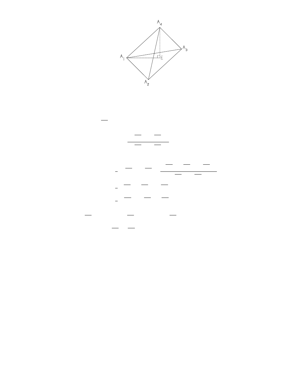
Hence A
4
E =
|
-
A
1
A
4
·X|, where X is a unit direction vector for the line
A
4
E. We can take
X =
-
A
1
A
2
×
-
A
1
A
3
||
-
A
1
A
2
×
-
A
1
A
3
||
.
Hence
vol A
1
A
2
A
3
A
4
=
1
6
||
-
A
1
A
2
×
-
A
1
A
3
||
|
-
A
1
A
4
·(
-
A
1
A
2
×
-
A
1
A
3
)
|
||
-
A
1
A
2
×
-
A
1
A
3
||
=
1
6
|
-
A
1
A
4
·(
-
A
1
A
2
×
-
A
1
A
3
)
|
=
1
6
|(
-
A
1
A
2
×
-
A
1
A
3
)
·
-
A
1
A
4
|.
19. We have
-
CB= [1, 4,
−1]
t
,
-
CD= [
−3, 3, 0]
t
,
-
AD= [3, 0, 3]
t
. Hence
-
CB
×
-
CD= 3i + 3j + 15k,
so the vector i + j + 5k is perpendicular to the plane BCD.
Now the plane BCD has equation x + y + 5z = 9, as B = (2, 2, 1) is on
the plane.
Also the line through A normal to plane BCD has equation
x
y
z
=
1
1
5
+ t
1
1
5
= (1 + t)
1
1
5
.
102

Hence x = 1 + t, y = 1 + t, z = 5(1 + t).
[We remark that this line meets plane BCD in a point E which is given
by a value of t found by solving
(1 + t) + (1 + t) + 5(5 + 5t) = 9.
So t =
−2/3 and E = (1/3, 1/3, 5/3).]
The distance from A to plane BCD is
|1 × 1 + 1 × 1 + 5 × 5 − 9|
1
2
+ 1
2
+ 5
2
=
18
√
27
= 2
√
3.
To find the distance between lines AD and BC, we first note that
(a) The equation of AD is
P
=
1
1
5
+ t
3
0
3
=
1 + 3t
1
5 + 3t
;
(b) The equation of BC is
Q
=
2
2
1
+ s
1
4
−1
=
2 + s
2 + 4s
1
− s
.
Then
-
P Q= [1 + s
− 3t, 1 + 4s, −4 − s − 3t]
t
and we find s and t by solving
the equations
-
P Q
·
-
AD= 0 and
-
P Q
·
-
BC= 0, or
(1 + s
− 3t)3 + (1 + 4s)0 + (−4 − s − 3t)3 = 0
(1 + s
− 3t) + 4(1 + 4s) − (−4 − s − 3t) = 0.
Hence t =
−1/2 = s.
Correspondingly, P = (
−1/2, 1, 7/2) and Q = (3/2, 0, 3/2).
Thus we have found the closest points P and Q on the respective lines
AD and BC. Finally the shortest distance between the lines is
P Q =
||
-
P Q
|| = 3.
103

@
@
@
@
@
¢
¢
¢
¢
¢
¢
¢
¢
¢
¢
©©
©©
©©
©©
©©
@
@
@
@
@
¢
¢
¢
¢
¢
¢
¢
¢
¢
¢
C
C
C
C
C
C
C
C
C
C
C
C
C
C
C
C
C
D
B
A
E
104
Wyszukiwarka
Podobne podstrony:
7 Tabela elementow rozliczenio Nieznany (2)
11 Wycinanie elementow obuwia z Nieznany (2)
Basic construction elements Voc Nieznany
Charakterystyka elementow kompu Nieznany
EN Tranzystory jako elementy dw Nieznany
15 Przygotowanie elementow do m Nieznany
Badanie uk adVw z elementami ni Nieznany (2)
16 Ksztaltowanie elementow narz Nieznany
MATERIALY NA ELEMENTY ZBIORNIKO Nieznany
Badanie obciazen elementow robo Nieznany
1 EL Solutions Elementary Progr Nieznany (3)
lab6 elementyAlgebryLiniowej id Nieznany
Dystrybucja jako element market Nieznany
Automatyka (wyk 10) elementy po Nieznany
1 Podstawowe elementyAid 9564 Nieznany (2)
3 1 Dla TR Sem3 Elementy Niezaw Nieznany
więcej podobnych podstron