GEOMETRY-BASED DETECTION OF

GEOMETRY-BASED

FLASH WORM DETECTION

A Writing Project

Presented to

The Faculty of the Department of

Computer Science

San Jose State University

In Partial Fulfillment

Of the Requirements for the Degree

Master of Science

Sang Soo Kim

December, 2006

Approved by:

Department of Computer Science

College of Science

San Jose State University

San Jose, CA

_________________________

Dr. Mark Stamp

_________________________

Dr. Chris Pollett

_________________________

Dr.

Agustin

Araya

Abstract

While traditional Internet worms take hours or days to infect a high percentage of

vulnerable hosts, a flash worm takes seconds. Because of the rapid rate at which flash

worms spread, existing worm defense mechanisms cannot respond fast enough to detect

and stop a flash worm infection.

In this project, we propose a geometric-based detection mechanism that can detect the

spread of flash worms in a short period of time without human intervention. We attempt to

detect network traffic patterns that are indicative of a flash worm attack in progress. We

have tested our approach on simulated flash worm traffic using more than 10,000 nodes. In

addition to testing on flash worm traffic, we also tested our method on realistic Internet

traffic to estimate the false alarm rate.

In order to efficiently analyze a large quantity of network traffic, we implemented an

application that converts network traffic data into a graphical form. Using this application

the analysis is done graphically with flash worm attacks appearing as tree structures.

Table of Contents

1. Introduction

2. Background

2.1. Common Structure of Flash Worms
2.2. Various Design Issues of Flash Worms

2.2.1. Spread Tree Topology

2.2.1.1. Shallow Spread Tree
2.2.1.2. Deep Spread Tree
2.2.1.3. Robust Spread Tree

2.2.2. Use of Threads

2.2.2.1. No Threads
2.2.2.2. Single Thread
2.2.2.3. Multiple Threads

2.2.3. TCP or UDP

2.3. Designing a New Flash Worm Implementation

3. Implementation of Geometry-based Detector

3.1. Flash Worm Simulation

3.1.1. Finding a Suitable Simulator
3.1.2. Extending Simulator to Flash Worms

3.1.2.1. Modified NS-2 Default Environments
3.1.2.2. A New Network Packet
3.1.2.3. Node and CenterNode Network Entities
3.1.2.4. Network Hierarchy Example

3.1.3. Configurable Parameters

3.2. Flash Worm Detection Mechanism

3.2.1. Geometry-based Flash Worm Detection
3.2.2. Extending NS2 to Flash Worm Detection

3.2.2.1. Node Structure
3.2.2.2. Double Linked-list Sorted by Timestamp
3.2.2.3. Array of Pointers to Node Sorted by Node ID
3.2.2.4. Dynamic Determination of Root Nodes
3.2.2.5. Dynamic Determination of Depth
3.2.2.6. Exiting Parent-Child Relationship
3.2.2.7. Parent-Child Loop Avoidance

3.2.3. Configurable Parameters

3.3. Post-analyzer

3.3.1. Nam (Network Animator)
3.3.2. Custom post-analyzer

List of Figures

Figure 1: Flash Worm Spread Pattern

Figure 2: Hit-list and Corresponding Spread Trees

Figure 3: Shallow Spread Tree Topology

Figure 4: Deep Spread Tree Topology

Figure 5: Robust Spread Tree Topology

Figure 6: Single Thread Usage

Figure 7: Network Topology of NS-2

Figure 8: Loop Avoidance

Figure 9: Nam Screen-shot

Figure 10: Sample Flash Worm Traffic

Figure 11: Complete Tree

Figure 12: Zoomed-in and ToolTip

Figure 13: Detection Mechanism in Action

Figure 14: Spread Tree of TCP traffic

Figure 15: Spread Tree of UDP traffic

1. Introduction

Since the early days of computer networks, computer worms have been developed,

often causing disruption on the network. As computer network architecture and Internet

security continue to advance to prevent the spread of worms, the worms continue to evolve

as well. Worm writers constantly strive to find ways to infect more hosts in less time.

It has been conjectured that a worm could be developed that would bring down the

entire Internet in less than 30 seconds [8]. Such a worm is termed a “flash worm”, and this

master’s project will consider a possible defense against flash worms.

The fastest worm to date was the Slammer worm, which infected “more than 90 percent

of vulnerable hosts within 10 minutes” [6]. The Slammer worm utilized a random scanning

strategy, in which infected hosts randomly select target addresses until all susceptible hosts

are infected. In a random scanning worm such as Slammer, the initial spread rate increases

exponentially, but the number of newly infected hosts diminishes later as the worm tries to

infect already infected hosts. These redundant infection attempts quickly clog up the

network bandwidth. Furthermore, if the random number generator used to determine

random target addresses has a defect, as was the case in the Slammer worm, the infection

may miss a portion of vulnerable hosts [6].

In order to spread faster and infect a higher percentage of vulnerable hosts, flash worms

must utilize a more effective search strategy. To date, flash worms are only theoretical in

the sense that no reported incidents have been filed. However there are many conjectured

flash worm implementations designed by various researchers. One conjectured

implementation is to pre-scan the entire Internet to generate a hit-list of all potentially

vulnerable hosts.

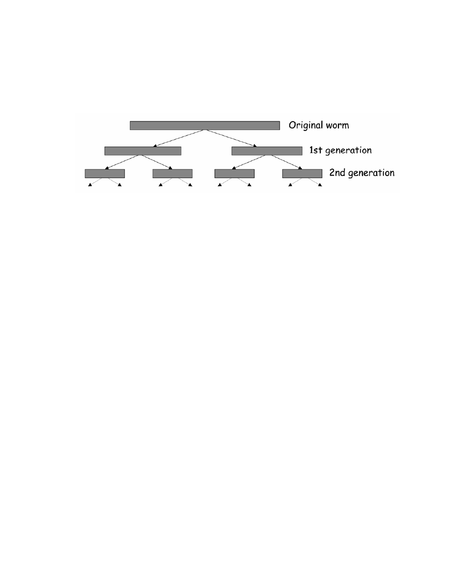
<Fig. 1: Flash Worm Spread Pattern> [19]

The initial worm includes the entire hit-list. Then upon each successful infection, the worm

divides its hit-list into n blocks, infects one address from each block, then communicates

the list of remaining addresses for each block to newly infected hosts [2]. This process

continues until all the addresses on the hit-list have been infected. In contrast to the

Slammer worm, this hit-list based flash worm does not scan for vulnerable target addresses

while spreading. Since searching for vulnerable target addresses is a slow process,

eliminating this process allows the unprecedented spread rate of the flash worm.

Because of the rapid speed at which a flash worm spreads, some of the prediction and

mitigation algorithms applicable to other worms are not appropriate for flash worms. In

this project, we propose a new geometry-based flash worm detection algorithm in which the

local network activity is monitored. Based on the monitored activity, we create a tree to

indicate the spread of a possible flash worm. This “spread tree” is designed to detect the

tree-like structure a flash worm is likely to use to propagate to the target host list. If the

depth of a spread tree reaches some predefined threshold, the network will automatically

shut down to prevent further spread of the flash worm. To avoid false alarms, the spread

tree must be pruned as well as updated periodically.

Prior work on the flash worm simulation and detection can be found in [19] and [20],

respectively. However, in [19] a simple Java simulator was used, while in this paper we

use a sophisticated NS2 packet-level simulation method. Also, the detection method used

in [20] relies on a simple count of the number of types of packets, whereas in this paper we

implement and analyze a novel geometry-based detection method.

In the remainder of this paper, we first describe the conjectured implementations of

flash worms in more detail. Section 2 discusses the essential components of a flash worm

implementation. Section 2 also explains how differentiating these components can result in

different infection behaviors. Section 3 details the design and implementation of our

proposed detection method. Section 4 shows our simulation test processes and the result.

Section 5 summarizes and presents our conclusions and a discussion of future work.

2. Background

Because there have been no incidents of flash worm outbreaks reported in the wild,

there is no example of an actual flash worm implementation. However, there are many

conjectured implementations of flash worms by various researchers. In this section, we

discuss several of these conjectured implementations.

2.1. Common Structure of Flash Worms

Despite various differences, every flash worm implementation is expected to have

the following common components:

• Hit-list

While traditional Internet worms scan for target hosts when they infect a

new host, flash worms do not perform this time-consuming process. Instead,

flash worms utilize a hit-list, which contains the list of all the target host

addresses.

Hit-list preparation process

Prior to instantiating the spread of flash worms, the worm author must

scan the entire Internet address to determine the vulnerable hosts. If the

author has a fast Internet connection and a high processing power, this

scanning can be done in a day [8]. However, to reduce the risk of being

detected by defense systems, the author may want to purposely slow

down the scanning process. Such stealthy scanning may take several

weeks.

Typical Size of a Host Address

Since most of the network hosts are in IPv4 domain at this time, the usual

number of bytes required to represent one host address is 32. That means,

a single UDP packet can store about 35 host addresses if the maximum

size of a UDP packet is 1200 bytes.

Low Failed Infection Attempts

In addition to increasing the spread speed, the use of a hit-list also

protects flash worms from some existing worm containment defenses.

For example, a containment defense that looks for unusually high

numbers of missed connections cannot detect the spread of flash worms

because most infection attempts are likely to succeed.

• Maximum Infection Number

Given a list of addresses to infect, each host does not infect all the listed

addresses. Instead, each host attempts to infect a small number of addresses

and propagates the remaining addresses to other hosts.

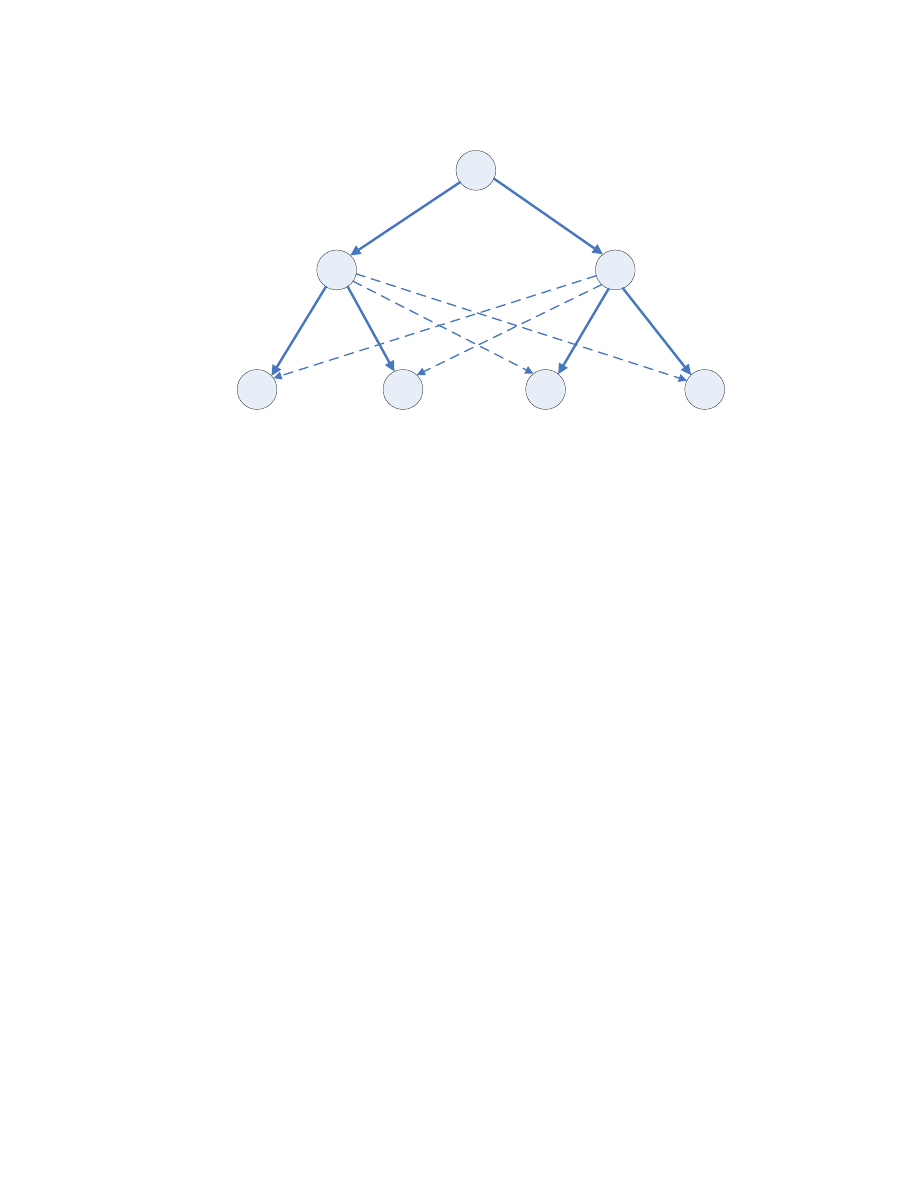
• Spread Tree

While the use of a hit-list enables the rapid spread rate of a flash worm, it

also implies that the flash worms spread following a tree-like pattern. We call

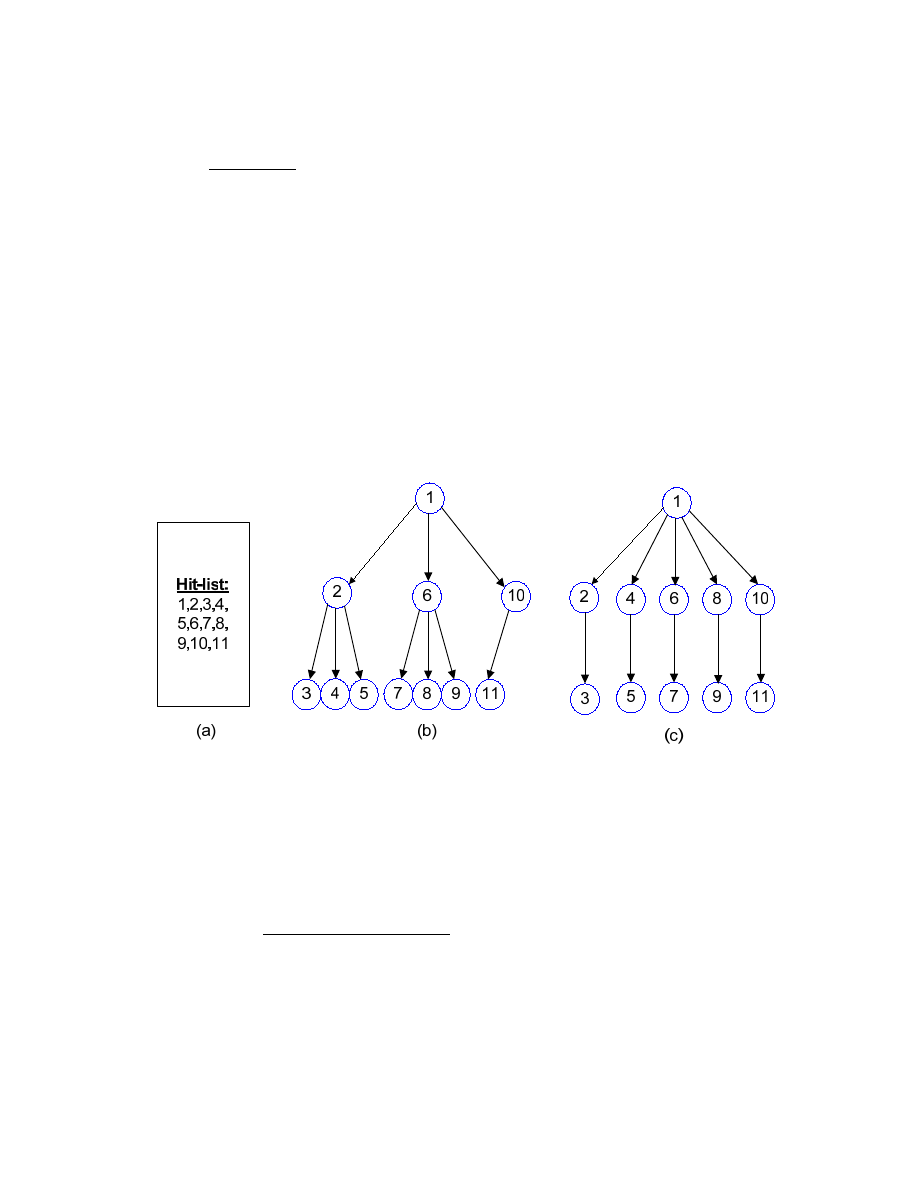
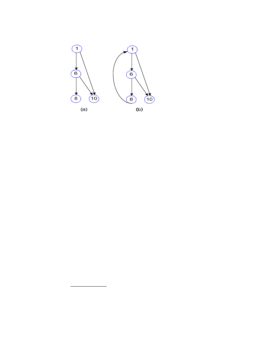
this spread pattern the spread tree. For example, the hit-list of Fig. 1 (a) with

maximum infection number of 3 creates the spread tree shown in Fig. 1 (b). In

the figure, Node 1 is infected first. Then Node 1 infects Nodes 2, 6, and 10.

The subsequent nodes infect up to 3 nodes as well, propagating the remaining

target addresses to other nodes.

<Fig. 2: Hit-list and 2 Corresponding Spread Trees>
(a) The hit-list contains 11 target addresses; (b) The spread tree formulation if each node attempts to
infect 3 other nodes at most; (c) Each node infects 5 nodes at most. Note that only node 1 has the enough
target addresses to infect 5 nodes.

At this point, defining some important components of spread trees is necessary.

Parent-Child Relationship

There is a one-to-one parent-child relationship if one host infects

another host. For example, in Fig (b) above, Node 6 is a parent

of Node 7, and Node 7 is a child of Node 6.

Depth (or Generation) Number

The depth of a node is the maximum length of the path from the

root to the node. In case a node has multiple parents, the

maximum length is assign to the node because our detection

mechanism is designed to trigger an alarm on the first sign of a

flash worm infection. On the other hand, if the minimum length

were assigned to the node, a triggered detection alarm would be

delayed and we wanted to avoid this delay. In Fig (b), for

example, Node 7 has depth of 2 and Node 10 has depth of 1.

The depth can also be called generation number. For example, in

Fig (b), Nodes 2, 6, and 10 are all in the same first generation.

The maximum number of generations required to infect N hosts

if each host infects K other hosts is given by

¾ O(log

For example, in Fig (b), the maximum generation number is

O(log

11) = 3.

Node Creation (or Infection) Time

Each node has an associated creation time. This is the time at

which the node was first infected by a flash worm. Note that the

nodes from the same generation should have similar creation

time since they are expected to be infected at about the same time.

Total Infection Time

The total infection time is the amount of time required to infect

all of the hosts listed in a hit-list. The total infection time is

equivalent to the node creation time of the last leaf node.

2.2. Various Design Issues of Flash Worms

When designing a flash worm, the worm author has to take the following issues into

account as they will characterize the worm infection behavior. Some of these may

actually be the by-products of the worm behavior, outside of the worm author’s

purposeful design.

2.2.1. Spread Tree Topology

The maximum number of attempt each host tries to infect defines the shape of

the spread tree. The authors of [7], who first published the work regarding flash

worms, have laid out these three spread tree topologies.

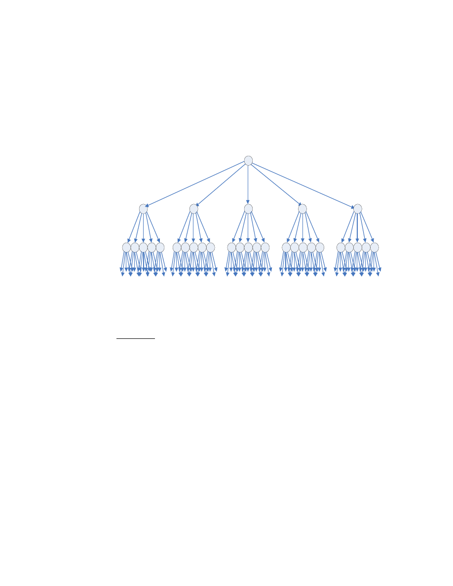
2.2.1.1. Shallow Spread Tree

In a shallow spread tree topology, each host tries to infect many other hosts.

As can be seen in Fig. 2 below, it takes 3 generations to infect 155 hosts if

each host attempts to infect 5 other hosts.

<Fig. 3: Shallow Spread Tree Topology>

Advantage:

Using a shallow spread tree it takes a short amount of time to infect all

of the target hosts since this topology requires a small number of generations.

If there is one root host with OC-12 connection which has a 750Mbps link, it

is claimed in [8] that such a shallow spread tree can infect 1,000,000

vulnerable hosts in less than 1 second. In this particular tree, it is structured

such that the first generation infects 5,000-50,000 hosts, and the second

generation infects 20-200 hosts. Thus, it takes only 2 generations to infect

1,000,000 hosts.

Furthermore, this topology is tolerant against a failed infection. A

network host may not get infected by a flash worm for many reasons. The

host may no longer have a security hole, or the infection packet may be lost.

Nevertheless, the problem is if a host is not infected, the hosts constituting

its child nodes in the spread tree will not get infected either. The shallow

spread tree topology is tolerant against such infection failures. For example,

in the Fig. 2 above, suppose one host from first generation fails to get

infected. Then, that means, only 1 out of 5 failed and we still have 4 other

hosts to continue the infections. Assuming no other hosts would fail, still

80% of the total hosts could get infected. Note also that if such a failure

occurs in later generations, there would be less uninfected hosts.

Disadvantage:

As each host tries to infect many other hosts, this topology places

significant computation burden on each host. Furthermore, the traditional

worm defense systems which look for sudden increase in the number of

network connections from a host may detect the worm activities.

2.2.1.2. Deep Spread Tree

In a deep spread tree topology, each host tries to infect only a small number

of other hosts. If we were to infect the same 155 hosts again using a deep

spread tree topology as illustrated in Fig 3, it would require 7 generations to

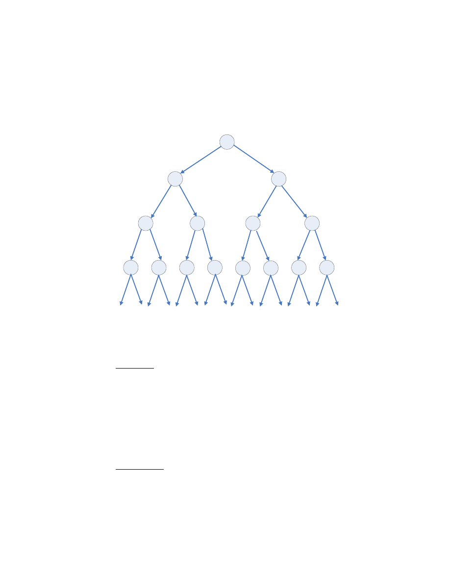
infect all nodes. Recall that the shallow spread tree discussed above would

require only 3 generations.

<Fig. 4: Deep Spread Tree Topology>

Advantage:

Since each host infects a small number of other hosts, the

aforementioned defense systems, which look for a sudden increase in the

number of network connections, would not be effective against this topology.

Disadvantage:

Compared to the shallow spread tree topology, this topology requires

more generations to infect the same number of target hosts. Since there is a

propagation delay in sending the target list from one generation to the next,

more generations imply a longer propagation delay. Therefore, this

topology takes a longer time to infect all of the target addresses.

Furthermore, if one node from the early generation fails to get infected,

the impact is larger than in the shallow spread tree. For example, in the Fig

3 above, if one node from generation 1 fails to be infected, then half of the

target addresses would not get infected.

♦ Note

The flash worm detection mechanism that we propose in this paper is most

effective only for a deep spread tree topology because the mechanism

requires that we see the spread tree grow to a certain depth.

2.2.1.3. Robust Spread Tree

One of the obvious difficulties in implementing flash worms is to obtain a

complete hit-list. Since the Internet continues to change as new hosts are

added and deleted, some infection attempts may fail. As discussed in the

deep spread tree topology section, if an infection attempt fails near the root

of the spread tree, then half of the spread tree may not be infected.

To provide a degree of resilience to the failed infection attempts, the

following topology can be used.

<Fig. 5: Robust Spread Tree Topology>

In this more robust topology, each host tries to infect its neighbor’s child

hosts. Even though this redundancy consumes some additional network

bandwidth and processing power, it protects the worm from a failure to

infect a particular node.

2.2.2. Use of Threads

In addition to defining the spread tree topology, the flash worm author would

need to decide whether to use threads. The use of threads at the application

layer can impact the total infection time.

2.2.2.1. No Threads

If threads are not used, then a host has to wait until it receives all the target

addresses from its parent. Until this is completed, the host cannot infect

other hosts. In other words, a task process to receive target lists and another

task process to infect target hosts cannot be run simultaneously if threads are

not used.

The hosts near the root node would expect to wait the longest because the

target address list is larger. On the other hand, as the host is closer to the

leaf nodes, the waiting time is expected to be significantly reduced.

♦ Note

Our simulation implementation of flash worms does not use threads.

Therefore, there are propagation delays which vary with respect to the size

of the target list.

2.2.2.2. Single Thread

In an implementation that can utilize a single thread, the host can create an

instance of a thread to infect its child node immediately after a target address

is received. That is, a thread can be used to receive the target list while

another thread can be used to infect and send the target list. The Fig. 5

illustrates the procedure.

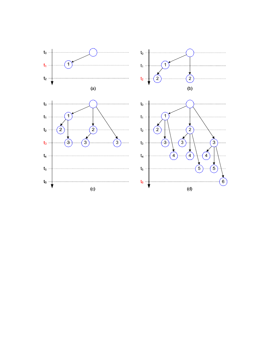
<Fig. 6: Single Thread Usage>
(a) At t

, the root node infects one other node; (b) At t

, the root node infects second node. The previous child

node has received a target address from the root node and is ready to infect another node. The node infects
another node by creating a thread. (Note that the node is still receiving the target list from its parent); (c) At t

three new nodes are infected; (d) At t

, all nodes are infected. [2]

In the example above, each node creates an instance of a thread every t

time.

By using a single thread, a node does not have to wait until it receives all the

target address, which significantly reduces the total infection time.

2.2.2.3. Multiple Threads

Multiple threads can be used in an environment where a node receives

multiple target addresses from multiple sources simultaneously. For

example, in a robust spread tree topology, a node may receive multiple

target addresses from different parent nodes. Therefore, a child node may

start different threads for each of the multiple worms it receives, which can

quickly snowball into X

threads at a depth of n and X maximum infection

number.

2.2.3. TCP or UDP

Another important decision a flash worm author has to make is whether to

use TCP or UDP. TCP establishes and maintains a connection before

transmitting the data, which requires more packets to be sent than UDP. On the

other hand, UDP does not establish a connection and data can be immediately

transmitted between two hosts. Therefore, a UDP-based flash worm can infect

faster than a TCP-based flash worm.

Even though the use of TCP can be slower than using UDP, the connection-

oriented nature of TCP provides guaranteed delivery of data whereas UDP does

not. As discussed in the spread tree topology section, failure to deliver infection

packets in the early stages of the worm infection can have a huge impact.

Therefore, the worm author has to balance the infection speed against the risk of

missed connections when choosing the network transmission protocol. It may be

best to use UDP for speed and build its own reliable delivery mechanism to avoid

missed infections in early generation.

♦ Note

Our simulation of flash worms uses UDP. We assume that only one UDP

packet is required to infect a target host. This is unrealistic for the early

generations of an infection, but it is a reasonable model for later generations.

2.3. Designing a New Flash Worm Implementation

While there are many existing hypothetical implementations of flash worms, there

may be other flash worm implementation designs still unknown. As an effort to

uncover such unknown designs, we propose a new flash worm implementation

below.

Central Hit-list Server based Design

• Instead of distributing the address list from a parent node to a child node, the

hit-list is available from a central server.

• When a new host is infected, it asks the central server for target addresses.

Once the central server receives a packet from a target address, it removes the

target address from the hit-list (because it knows that the target address is

already infected).

• For simplicity and efficiency, we use UDP packets. Assuming a UDP packet

can store 1200 bytes, a single UDP packet can store about 35 IP Addresses.

That means, a simple Request-Reply UDP packets will get 35 target lists from

the server.

• Advantage:

The central server can efficiently distribute the hit-list

This design eliminates the initial delay in propagating a large hit-

list

This design is also resilient to failed infections; if a node fails to

get infected, other node will infect its child nodes.

The hit-list can be updated dynamically as new vulnerable addresses are

added. Also, incorrect addresses can be removed after some timeout.

The current infection progress state can be monitored in real time.

• Disadvantage:

The hit-list server can be relatively heavily loaded.

3. Implementation of Geometry-based Detector

In this section, we discuss how we implemented a simulator to generate the flash worm

traffic. Then, we discuss how we developed a new application to graphically analyze

the flash worm traffic and to test our proposed detection mechanism.

3.1. Flash Worm Simulation

3.1.1. Finding a Suitable Simulator

In order to study the defense against flash worms, we needed to have a

simulator to simulate the behavior of flash worms. Because learning to use a new

simulator in depth is a difficult and often time-consuming process, we wanted to

verify that a specific simulator is capable of simulating many nodes and generating

the packet-level traffic prior to learning the simulator in depth.

List of Simulators:

The following are simulators that can simulate a vast number of nodes:

1) Scalable Simulation Framework [14]

Scalable Simulation Framework has been outdated. The latest simulator

update was in year 2004.

2) Simnet [15]

Simnet was designed mainly for analyzing network security protocols.

Although an implementation of a worm model was available, the simulator

did not have detailed documentation.

3) OPNET [16]

Opnet was a commercial-quality network simulator product. A student

license was available that required a complex registration.

4) GTNetS [17]

GTNetS was a network simulator developed from Georgia Tech University.

The simulator was complex to install and use.

5) NS-2 [18]

Developed and maintained by various research orginations, NS-2 was

widely used in academic works. Although NS-2 was well documented, it

was also very complex to use.

Although it seemed to be very complex to use at first, we decided to use NS-

2 because it was easy to install and had some forms of the user documentation.

However, the other simulators could have been used to do the project as well.

3.1.2. Extending the Simulator to Simulate the Spread of Flash Worms

3.1.2.1. Modified NS-2 Default Environments

• By default, NS-2 uses a flat-routing scheme, in which every node knows

the address of every other node, resulting in a routing table size to the

order of n

for n nodes. To reduce the memory requirement of

simulations over large network topologies, we created a hierarchical-

routing scheme. For hierarchical-routing, each node knows only about

those nodes in its level. Thus, the routing table size was reduced to the

order of log n.

3.1.2.2. Added a New Network Packet:

We enhanced NS-2 to support the following new network packet:

• Packet Format

struct

hdr_fworm {

nsaddr_t

dst;

nsaddr_t

src;

nsaddr_t

target_range_first;

nsaddr_t

target_range_last;

};

There are four fields in the packet

dst = packet destination address

src = source address

target_range_first = first range of address to infect

target_range_last = last range of address to infects

Instead of transmitting each target address of the hit-list, we

decided to send the range representing the list. So, a single

packet can infect and propagate the target addresses. The

propagation delay to transmit the target addresses is simulated by

forcing infected host to wait for the estimated delay before

infecting other hosts. The delay varies with respect to the range

size.

3.1.2.3. Added Two New Network Entities: Node and CenterNode

The entity Node represents a host that is vulnerable to flash worm

infections.

The entity CenterNode is a special node that is not vulnerable to flash

worm infections. It is located at the center of the network hierarchy, and

it acts as a router to forward flash worm packets amongst Nodes. Every

flash worm data has to go through this entity first. Since it can see all

the flash worm traffic, it is also the ideal place to implement our

detection mechanism.

The entities Node and CentorNode provide a global view of a large

network topology. While this might not seem too realistic, similar

structure can be formulated on a LAN or a WAN. In any case, we are

trying to see if our detection mechanism can work in principle.

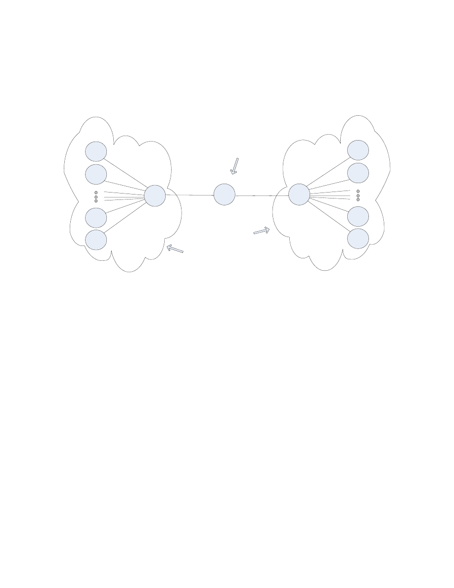
3.1.2.4. Network Hierarchy Example

Fig. 6 displays an example of simulated network topology in NS-2.

0.0.0

0.1.0

0.1.126

0.1.127

0.1.1

0.1.2

0.2.0

0.2126

0.2127

0.2.1

0.2.2

Cluster 2

Cluster 1

CenterNode

<Fig. 7: Network Topology of NS-2, Consisting of Two Clusters>

There is always one CenterNode in the topology, which has the address

0.0.0 and is located at the center.

Every packet is sent to CenterNode first. Then, the CenterNode

forwards the packet to the correct destination.

Each cluster can have maximum of 128 nodes.

Of the address form 0.X.Y, X represents the cluster number and Y

represents the node ID within the cluster.

A node with the address form of 0.X.0 is a head of the cluster.

Both the CenterNode and the head of a cluster have enough buffer size

to handle large network traffic.

3.1.3. Configurable Parameters

Following are the configurable parameters to simulate various flash worm

scenarios:

Number of Clusters

The simulator can support up to 100 clusters. Since each cluster

has 128 nodes, this means that the simulator can simulate 12,800

nodes.

Our simulation has been performed on a computer with 1GB of

RAM. A computer with higher RAM space should be able to

simulate more than 100 clusters.

Infection Number

This is the maximum number that each host tries to infect other

hosts.

Link Delay

There is a network propagation delay between the CenterNode

and the head of a cluster. Unless otherwise specified, we use

5ms as the default delay.

There is also a network propagation delay between nodes and the

head of the nodes. Unless otherwise specified, we use 10ms as

the default delay.

If using the default delay values, the end-to-end propagation

delay between 2 end-to-end hosts is 10 + 5 + 5 + 10 = 30 ms.

3.2. Flash Worm Detection Mechanism

To discuss our detection mechanism, there are underline assumptions to consider.

First, there are at least one thousand hosts that are vulnerable to flash worm infections.

Second, every host makes the same number of infections. Third, the infected hosts

create deep spread tree. Last, all infection attempts are successful.

Since flash worms spread rapidly, the traditional signature-based defenses or

manual human intervention cannot respond in adequate time to stop the flash worm

propagation. Therefore, much effort has gone into designing automated flash worm

containment mechanisms. Besides the one we are proposing in this paper, there are two

other common defense mechanisms against flash worms:

The author of [1] proposes a defense system against flash worm in which the

addresses of the Internet hosts are changed frequently. By doing so, the goal is to make

the hit-list, which is pre-generated by the flash worm authors, unreliable and unusable.

However, the mechanism requires a significant modification of the existing Internet

infrastructure.

The second defense mechanism is to utilize a honeypot. Traditionally, a honeypot

is a fake network environment where various viruses and worms can be trapped. If the

address of a honeypot is in the hit-list, attempting to infect the honeypot may prevent a

part of the spread tree from getting infected. However, as discussed in the robust

spread tree topology section, there are ways to get around this trap.

3.2.1. Geometry-based Detection of Flash Worms

3.2.1.1. Basic Idea

The basic idea of our work is to create a spread tree by monitoring network

traffic activities and shutting down the network if a predefined threshold

level of depth is reached. The spread tree is pruned periodically by

removing the old nodes so that the tree would not grow continuously and

trigger false alarms. By carefully choosing the threshold depth and the

prune period, it should be difficult to trigger the false alarm by non-flash

worm packets.

3.2.2. Extending NS2 to Simulate Detection of Flash Worms

3.2.2.1. Node Structure

In order to create the spread tree, we use the following tree node structure:

• struct node {

int nodeID;

// ID (or address) of this node

int depth;

// depth (or generation) number

double timestamp; // node creation time

node ** children; // list of children

node ** parent; // list of parents

int numChildren; // number of children

int numParent;

// number of parents

int maxChildren; // max number of children

int maxParent;

// max number of children

node * before;

// for list sorted by time

node * after;

// for list sorted by time

};

Note that our node implementation can support multiple parents.

This late added feature required more complex computation to be

performed dynamically. For example, it required the support of

parent-child loop avoidance and recursive depth determination which

are discussed below. If the node were to support only one parent, the

implementation could have been much simpler.

3.2.2.2. Double Linked-list Sorted by Timestamp

To minimize the cost of updating the tree structure, we used the following

double linked-list sorted by timestamp:

Linked-list

Node 6

Time: 13

Node 1

Time: 10

By using this linked-list, there is no need to search for old nodes in

the pruning process.

Remove
nodes starting
from head

Add new
nodes starting
from tail

Although a simple single-linked list could have used for this purpose,

we used double-linked list in case the items may have to be sorted.

For example, if the infection time is changeable, then the list has to

be updated by sorting. See section 3.2.3.6 for more discussion on

this issue.

3.2.2.3. Array of Pointers to Node Sorted by Node ID

To allow us to easily access the node structure, we created an array of

pointers to node structure that is sorted by Node ID.

Node * pNodes[size of max node];

For example, given the a nodeID X, we could access the node

structure by

*pNodes[X]

3.2.2.4. Dynamic Determination of Root Nodes

Through out the operation, there can be many splits or merges of spread

trees. For example, a tree is split if the root node is removed; two trees are

merged if one node infects one node on the other tree. Since it would be

very cumbersome to maintain a list of all the root nodes, we decided to

maintain no explicit list of root nodes. Instead, if the parent number of a

node is 0, the node is the root.

3.2.2.5. Dynamic Determination of Depth

Instead of updating the depth of every child node when the depth of a parent

node is changed, depth is determined recursively as following:

depth = maximum depth of parents + 1

3.2.2.6. Exiting Parent-Child Relationship

If there is an existing parent-child relationship between two nodes when

creating a new relationship, we decided to do nothing. Alternatively, we could

have updated the node creation time so that the node would be pruned at a later

time. However, we thought doing so would consume significant computation

power to reorganize the linked-list. For example, if two nodes are

communicating using a TCP connection or running some application, there

would be many rapid requests to update the node creation time in a short period

of time. Therefore, we decided that it would be better not to update the node

creation time.

3.2.2.7. Parent-Child Loop Avoidance

Before a new parent-child relationship is created, a check is performed to

prevent the formation of a parent-child loop. See Fig. 7 below.

<Fig. 8: Loop Avoidance>
(a) No loop; (b) There is a loop, connecting node 1,6, 8

In Fig 7(a), there is no loop. However, in Fig 7(b) there is a loop among the

nodes 1, 6, and 8. If there is a loop, we cannot determine the depth correctly

since we cannot determine which node is the parent/root node. Therefore, if

a new parent-child relation creates a loop, we remove that relationship right

away. There can be potential attacks against this restriction, one of which

we discuss later.

3.2.3. Configurable Parameters

Similar to the configurable parameters in flash worm simulation, there are

configurable parameters for detection mechanism.

Depth Threshold

This is the maximum number of depth allowed before an alarm is

triggered to notify that spread of flash worms has detected.

Too lower number is likely to generate many false alarms; too high

number would not detect flash worm early enough to react.

Prune Period

This is the amount of time elapsed before next pruning occurs.

Prune Amount

This is the amount of time we subtract from the current time, and any

nodes created before that time is pruned. For example, if Prune

Amount is 5 seconds and current time is 30 seconds, the nodes with

creation time less than 30 – 5 = 25 seconds will be removed from the

spread tree.

3.3. Post-analyzer

In this section we discuss how we implemented a post-analyzer to help visualizing

the simulated result.

3.3.1. Nam (Network Animator)

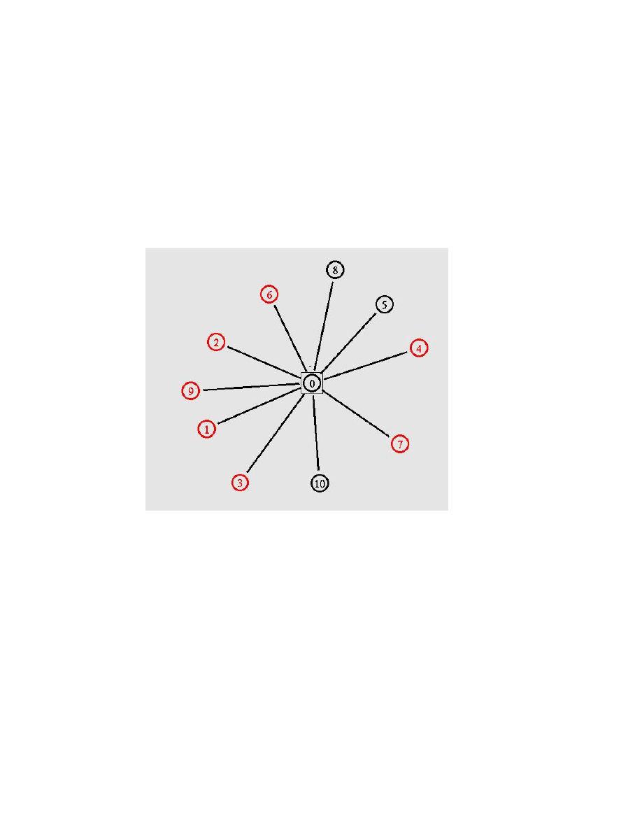
NS-2 provides Nam, which is a graphical utility to display the network topology

and simple network traffic activities. We have implemented Nam such that when a

node is infected, the color of the node changes to red. Following is a sample output

of running the simulation consisting of 10 nodes.

nam result

<Fig. 9: Nam screen-shot>

Node0 is the CentralNode

Nodes 1,2,3,4,6,7,9 have been infected at the time

Nodes 5,8,10 have not been infected yet.

This is a screen shot of a specific simulation time; eventually, every node

will get infected.

Disadvantages:

If plotting a lot of nodes, Nam cannot position nodes evenly across

the screen. Nam will display all the nodes close to the CenterNode

and we will eventually see a big dark circle in the middle.

Nam cannot automatically order the nodes into a tree form.

3.3.2. Custom Post-analyzer

To resolve all Nam’s shortcomings, we have implemented a custom post-

analyzer using MFC from Microsoft Visual Studio. Following are the features of

the post-analyzer:

Able to plot a vast number of nodes on a screen

Able to zoom in (or out) to see detailed structure

Able to see detailed information of a node when the mouse is placed over

the node

The information is displayed in a tooltip

• The information is consisted of node address, node creation

time, and depth. The tooltip can be easily modified to display

more information.

Able to manually start, stop, and rerun the simulation at any time.

Able to run the detection mechanism

The detection mechanism is implemented in both NS-2 and the post-

analyzer. The detection mechanism in NS-2 can be used to monitor

the flash worm packets as soon as they are generated by the

simulator. However, the configurable parameter for the detection

mechanism such as Prune Period cannot be changed after the

simulator is started and the testing of the detection mechanism

always requires regeneration of flash worm traffic. On the other

hand using the post-analyzer, the configurable parameters of the

detection mechanism can be changed and tested at any time. The

post-analyzer can also apply the detection mechanism on saved flash

worm traffic so the flash worm traffic does not need to be

regenerated. Therefore, we prefer to use NS-2 only to generate the

flash worm traffic and run the detection mechanism on the post-

analyzer.

4. Tests and Results

In this section we explain our testing setup and provide an analysis on the result.

4.1. Generate flash worm traffic

Flash worm traffic was generated by running NS-2 simulator with following

parameters:

• Configurable Parameters:

Number of clusters = 10

Infection number = 2

• We disabled the detection mechanism of the simulator. If the detection

mechanism is disabled, NS-2 automatically outputs all the flash worm traffic

data into a text file.

• Traffic Format:

The traffic is organized by the following fields:

Event Time (in ms), Node Address, Parent Node Address, Target

Address Size

Each field is separated by a space.

For example, Fig. 9 displays the first five flash worm data.

line 1:

0.1 128 0 1279

line 2:

19.2 768 128 639

line 3:

19.2 129 128 638

line 4:

28.8 769 768 318

line 5:

28.8 1088 768 319

<Fig. 10: Sample Flash Worm Traffic>

Line 1 has the initial flash worm data. The line “0.1 128 0 1279”

means “Node 128 was infected by Node 0 at time 0.1 and the

target address size is 1279”. Since we simulate 10 clusters and

each cluster has 128 nodes, the initial hit-list size of 1279 is

correct.

Line 2 and 3 shows that Node 128 correctly infected 2 other

nodes at 19.2 ms. Note that the target address list is divided into

639 and 638 and distributed to Nodes 768 and 129 respectively.

Since our simulation does not utilize threads, the node has to wait

until it receives all the target addresses from its parent. From line

1 and 2, we can see that it took 19.2 – 0.1 = 19.1 ms to transmit

target list size of 639 from Node 128 to Node 768. Also, from

line 2 and line 4, we can see that it took 28.8 – 19.2 = 9.6 ms to

transmit target list size of 318 from Node 768 to Node 769.

Therefore, a higher propagation delay is required to transmit a

larger target list.

4.2. Plot and Analyze Flash Worm Traffic

After generating the flash worm traffic, we plotted and analyzed the traffic using

our post-analyzer.

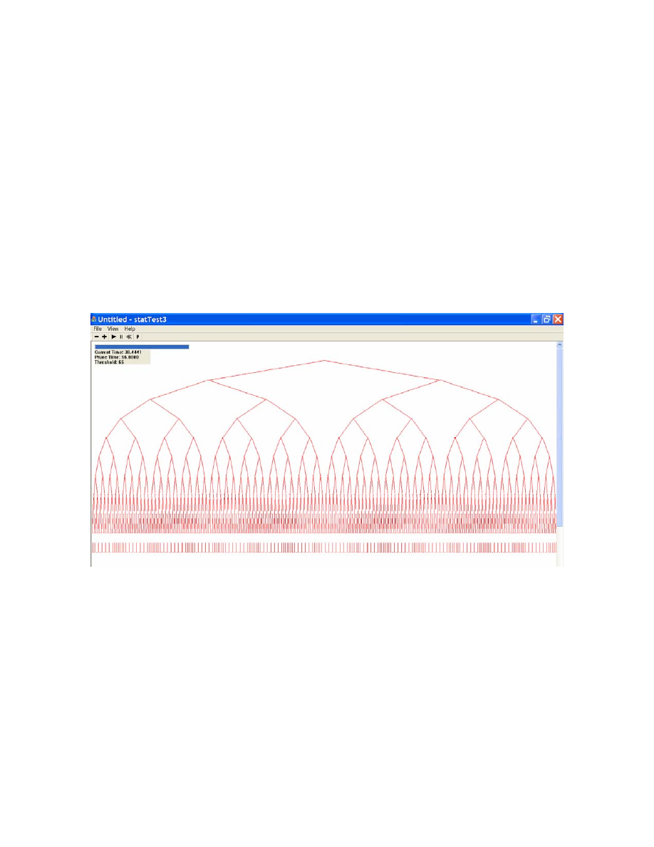
• Spread Tree Topology

Fig. 10 displays all the 1280 target nodes organized into a spread tree

topology.

<Fig. 11: Complete Tree>
Without Pruning

In this test setup, there is no pruning because we specified

sufficiently long pruning time period to display the complete tree

structure.

Fig. 11 displays a zoomed-in screen shot. It also shows a tooltip, which

describes the detailed information regarding Node 854.

<Fig. 12: Zoomed-in and ToolTip>

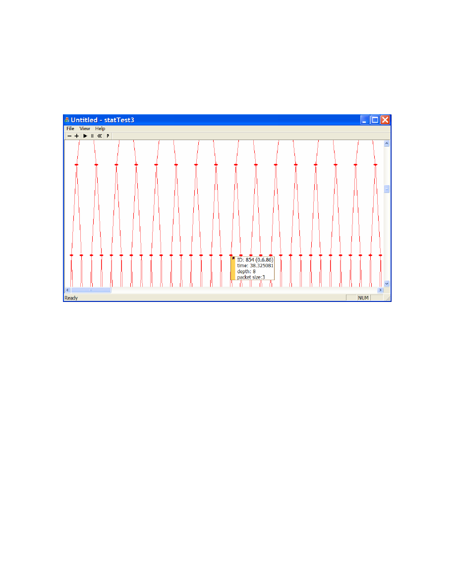
• Running Detection Method

Fig. 12 shows that our detection method found the spread of flash worms.

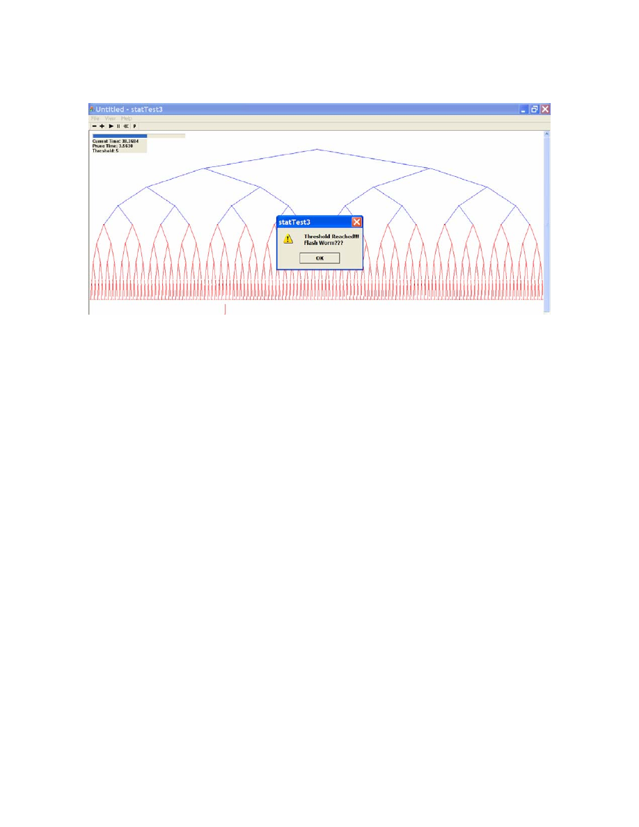
<Fig. 13: Detection Mechanism in Action>

For the detection method parameters, Prune Time is set to 3.5630 and

Threshold Depth is set to 5.

The nodes and lines marked in blue color indicate the pruned entities. In

the above example, the first 3 generations have been pruned.

4.3. Plot and Analyze the Actual Internet Traffic Captured from Lawrence

National Laboratory

• In the previous experiment, we tested that our detection mechanism can

successfully detect the spread of flash worms. However, we were also

interested to find out how the detection mechanism would respond to the other

network traffic.

• Instead of generating various Internet traffic as we generated the flash worm

traffic, we decided to use an archived Internet trace data from [9]. Captured

from the Lawrence National Laboratory using tcpdump of an actual WAN

traffic, the trace data went through a sanitization script to renumber IP addresses

and to remove all private packet contents. The sanitization script also separated

TCP traffic from UDP traffic and places them into different files. One can

capture one’s own Internet traffic using tcpdump and use the same sanitization

script to produce the similar trace data.

• There are more than 10 archived Internet traces available at the site. The trace

file we used for our testing below is called LBL-PKT. It contains an hour's

worth of all wide-area traffic between the Lawrence Berkeley Laboratory and

the rest of the world, started from 14:00 and ended at 15:00 on January 21, 1994.

• Traffic Format:

The traffic is organized by the following fields:

Timestamp of packet arrival, Source host, Destination host,

Source port, Destination port, Packet size

We modified our post-analyzer to use above fields to create spread trees.

We did not utilize the port numbers to create different spread trees for

different port number. However, in a real world deployment of our

detection mechanism, the spread trees should be further separated by the

port number because flash worms will probably use a specific port

number to spread.

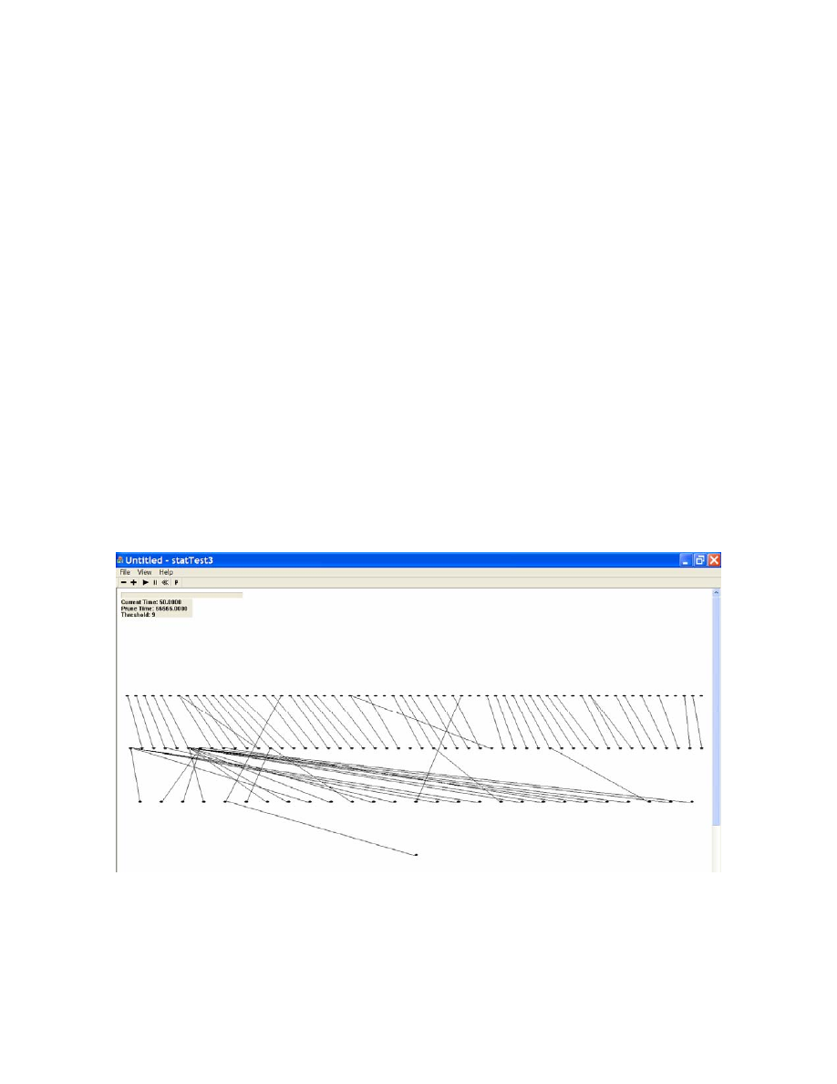
• TCP Traffic

The spread tree formulation of the TCP traffic is shown in Fig. 13. Even

though more than 150 packet events were processed, there were many

attempts to create loops or to create repetitive relationships. The

attempts to create loop were avoided and the attempts to recreate

existing parent-child relationship were ignored. Therefore, we did not

see rapid growth of the spread tree.

The tree structure seemed to be the reserved formulation of the flash

worm spread tree. The total number of nodes in a generation decreases

as generation number increases. However, the exact opposite happens in

flash worm spread tree.

<Fig. 14: Spread Tree of TCP traffic>

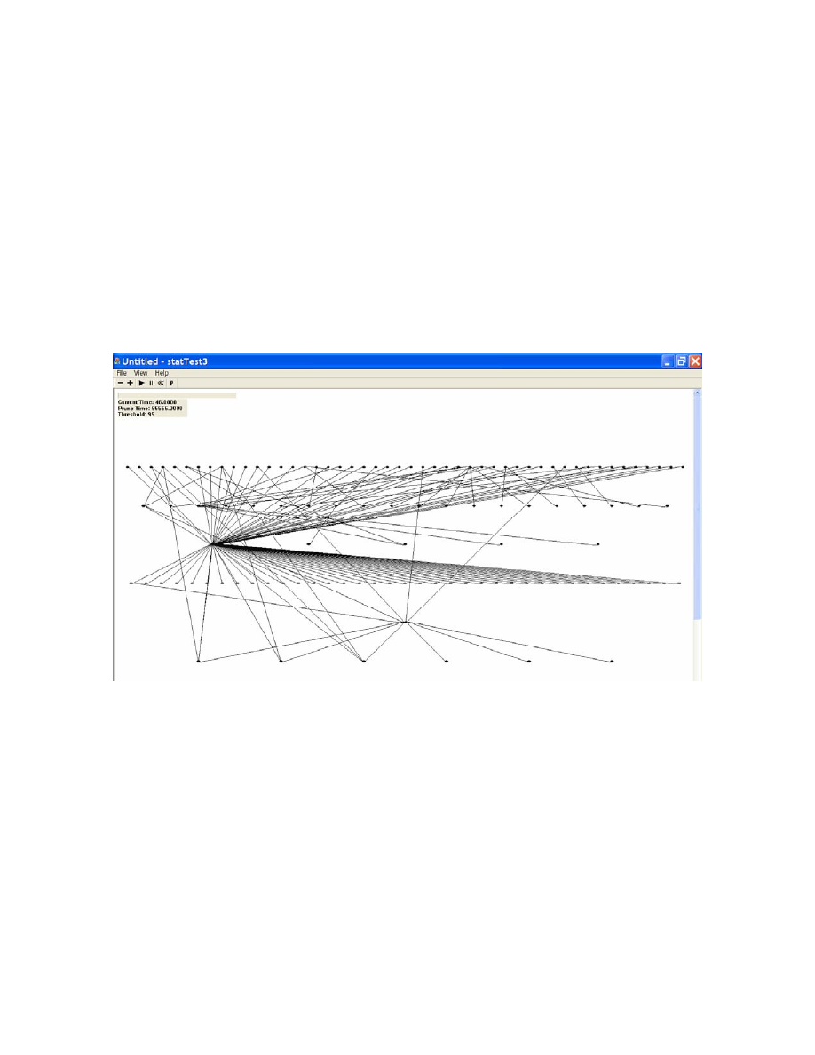
• UDP Traffic

In TCP traffic, many network communications were between 2 nodes.

However, in UDP traffic, we saw more interactions among different

nodes. See Fig. 14.

This time we processed about 300 packet events, but still it only created

5 generations.

<Fig. 15:

Spread Tree of UDP traffic

4.4. Breaking our Detection Mechanism

From the previous section, we saw that typical Internet traffic is not likely to trigger

false detection alarms. However, there are ways to break our detection mechanism:

• Slow down the infection process

Because nodes are pruned periodically, slowing down the infection

process with respect to the pruning period, the depth of the spread tree

may not grow rapidly.

As a counter-measure, the detection mechanism can look for growing

bursts of packets. Since flash worms transmit much higher number of

infection packets from a generation to the next, we could use this

characteristic to detect the spread of flash worms.

To address our counter-measure, a flash worm can be implemented to

transmit fixed number of infection packets per prune period. However,

such a flash worm would take significantly long time to spread that other

traditional signature-based detections can be used.

• Use customized source and destination addresses

An attacker can transmit customized packets in a way that makes the

flash worm packets be ignored. This attack is possible due to our

restriction that does not allow loops in the tree. For example, before

sending a packet to infect a node from next generation, source and

destination address fields can be switched to create a reverse parent-child

relation in the tree first. When the actual flash worm packet is processed

later, it will attempt to create a loop and will be removed.

As a counter-measure, the Internet infrastructure can be reorganized to

prevent or detection such customized packets. For example, the routers

can determine if a packet is originated from a network place but is

destined to forward to the same network.

• Fake flash worm traffic

An attacker can generate some harmless packets that would simulate the

geometry closely enough to make the detector shut down the network.

However, it would require a high computing power and a fast network

connection to generate the massive amount of flash worm packets in a

short period of time. Furthermore, since the attacker would be

generating customized packets as discussed above, the same counter-

measure is applicable for this attack.

5. Conclusion

In this project, we developed a simulator to generate flash worm traffic. We then,

developed an analyzer that can run our proposed geometric-based detection mechanism on

the traffic. We also tested our analyzer on real network traffic. Our results show that the

detection mechanism can be sensitive to the presence of the flash worm traffic while

maintaining insensitivity to other regular Internet traffic. Consequently, we believe that our

detection mechanism can successfully identify the spread of flash worms.

6. Future Work

First of all, in order to increase the maximum number of nodes simulated, a

different version of NS simulator can be used. PDNS [20], for example, is a network

simulator that can support parallel and distributed simulation over multiple PCs. The need

to simulate larger network topology may arise when testing our detection mechanism on a

shallow spread tree topology. Our current maximum of 10,000 nodes is not sufficient to

create flash worm traffic with a high infection number. For example, if each host infects 10

other hosts, it takes only 4 generations to infect all 10,000 nodes.

Secondly, more components can be used to identify the unique characteristic of the

flash worm spread tree and, thus, reduce the occurrence of false alarms. In our current

construction of the spread tree, we use depth as the only determining factor to decide

whether a flash worm outbreak has occurred. However, studies can be conducted to find

other factors. For example, there is a pattern that the total number of nodes in a generation

increases from a generation to the next. It follows the form X

, where X is the maximum

infection number and G is the generation number. Such a pattern may be used to reduce

false alarms.

As another effort to reduce the false alarms, research can be done on integrating

packet classification technology into our detection mechanism. The ultimate goal is to help

identify the well known application traffic patterns so that the known “safe” network traffic

would not be processed into a spread tree. As an example, we suspect that peer-to-peer

query flooding traffic is likely to trigger false alarms because of the many parent-child

relationships amongst a vast number of peers. If the packet classification technology can

identify such peer-to-peer traffic, then the traffic would not be processed by our detection

mechanism, thereby reducing the number of false alarms.

Bibliography

[1] S. Antonatos, P. Akritidis, E. P. Markatos, K. G. Anagnostakis, “Defending against

Hitlist Worms using Network Address Space Randomization.”

[2] Yuy Bulygin, “A spread model of flash worms”,

http://isiom.wssrl.org/index.php?option=com_docman&task=doc_download&gid=14

[3] Cheetancheri. "Modelling a Computer Worm Defense System."

http://seclab.cs.ucdavis.edu/papers/Cheetancheri-thesis.ps

[4] Ellis, Aiken, Attwood, Tenaglia. "A Behavioral Approach to Worm Detection."

http://www.wormblog.com/2005/03/a_behavioral_ap.html

[5] Goldi, Hiestand. "Scan Detection Based Identification of Worm-Infected Hosts."

http://www.tik.ee.ethz.ch/~ddosvax/sada/ScanDetection_ma_ws2004_2005.pdf

[6] Moore, Paxson, Savage, Shannon, Staniford, Weaver. “The Spread of the

Sapphire/Slammer Worm.”

http://www.caida.org/publications/papers/2003/sapphire/sapphire.html

[7] S. Staniford, V. Paxson, and N. Weaver, “How to Own the Internet in Your Spare

Time,” in Proceedings of the 11th USENIX Security Symposium (Security’02), San

Francisco, CA, pp. 149-167, Aug. 2002,

http://www.icir.org/vern/papers/cdc-usenix-sec02/

[8] S. Staniford, V. Paxson, and N. Weaver, “Top Speed of Flash Worms,” in Proceedings

of the 2nd ACM Workshop on Rapid Malcode (WORM), 2004,

http://www.caida.org/outreach/papers/2004/topspeedworms/topspeed-worm04.pdf

[9] The Internet Traffic Archive,

http://ita.ee.lbl.gov/

[10] Vogt. "Simulating and Optimising worm propagation algorithms."

http://web.lemuria.org/security/WormPropagation.pdf

[11] Weaver, Staniford, Paxson. "Very Fast Containment of Scanning Worms."

http://www.icsi.berkeley.edu/~nweaver/containment/containment.pdf

[12] Worm Blog by J. Nazario,

http://www.wormblog.com

[13] Wu, Vangala, Gao. "An Effective Architecture and Algorithm for Detecting Worms

with Various Scan Techniques."

http://www-unix.ecs.umass.edu/~lgao/ndss04.pdf

[14] Scalable Simulation Framework,

http://www.ssfnet.org/homePage.html

[15] Simnet,

http://simnet1.isi.jhu.edu/

[16] Opnet,

http://www.opnet.com/

[17] GTNets,

http://www.ece.gatech.edu/research/labs/MANIACS/GTNetS/

[18] The Network Simulator –NS2,

http://www.isi.edu/nsnam/ns/

[19] M. Stamp, "Information Security: Principles and Practice", Wiley-Interscience, 2005.

[20] PDNS - Parallel/Distributed NS,

http://www.cc.gatech.edu/computing/compass/pdns/

[21] Y. Li, Anomaly based detection of flash worms, Fall 2005.

[22] T. Nikl, Flash worm simulation and detection, Spring 2005.