
1
Classification of costs and
mathematics for budgets
Chapter
1

2
1.1
Introduction to financial information
Financial Accounting
(External information)
Financial accounts are produced mainly for external
users e.g. shareholders or investors. These are
normally published annually by a company. Internal
management would still use this information to
monitor the historic performance of the company.
The primary financial statements would normally
include an income statement, balance sheet and cash
flow statement.
These published accounts show the summary of all
financial transactions recorded, according to external
accounting laws and regulations. These financial
accounts show how much profit or loss has been made
for a period, what the assets and liabilities are and how
much cash has been generated by the company.
Management Accounting
(Internal information)
Management accounts are produced for internal users
of financial information within an organisation e.g.
directors and management.
There is no legal requirement or legal format for
how management accounting information should
be presented; it can be either provided ad-hoc or
periodically depending on the needs of internal users.
Management accounts are used for
Planning e.g. preparation of budgets for short
and long-term forecasting
Monitoring and controlling e.g. monitoring
the cost of different products or departments
Decision making e.g. pricing, break-even
analysis or maximising profit
3
1.2
Direct, variable or prime cost
Expenditure which can be economically identified with and specifically measured in
respect to a relevant cost object.
A cost that varies with a measure of activity. (CIMA)
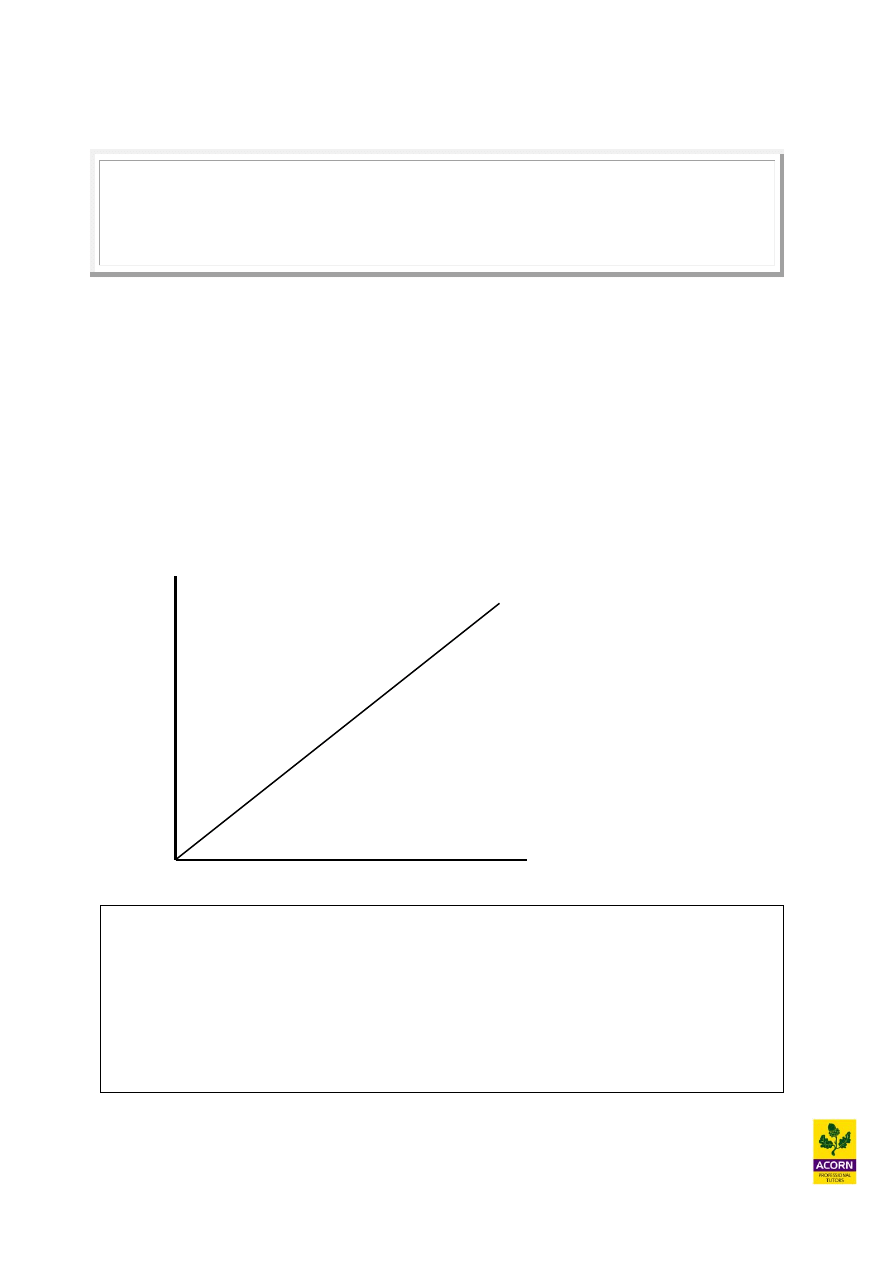
A direct cost or variable cost is a cost that can be easily identified or related to a cost per
unit or activity level of some kind e.g. a cost which rises or falls directly with the
production/provision of a good or service within an organisation. Examples could include
labour piece work schemes e.g. a factory worker that gets paid for each unit they make or the
cost of material/components for the production or assembly of a product.
The total direct cost of production is referred to as ‘prime cost’.
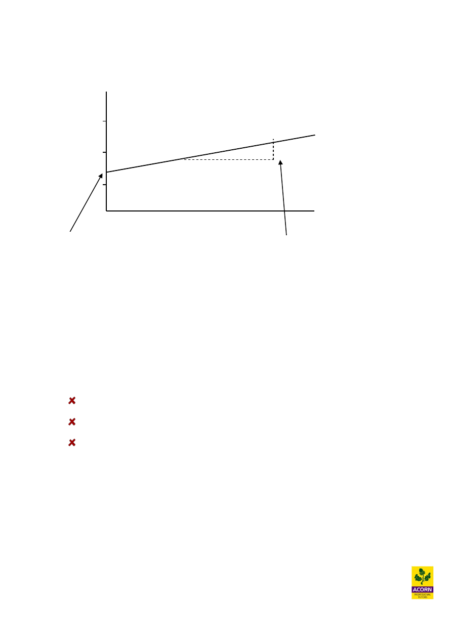
All variable cost starts from the origin of the graph indicating the cost is nil if the activity
level is zero. Variable cost does not necessarily behave in a linear manner as depicted below
e.g. a constant amount incurred for each unit of activity. It can behave in a curvilinear (non-
linear) manner as well, in which case the variable cost line below would be curved not
straight.
Example 1.1
A cost unit is a product, service, activity or output of some kind in which costs can be
ascertained, give three examples of a cost per unit that could be used for a hospital?
Cost
(£)
Direct or variable cost
Output or activity level (units)
4
1.3
Indirect or fixed cost
Expenditure which cannot be economically identified with a specific saleable cost unit.
A cost incurred for an accounting period, that within certain output or turnover limits,
tends to be unaffected by fluctuations in the level of activity (output or turnover).
(CIMA)
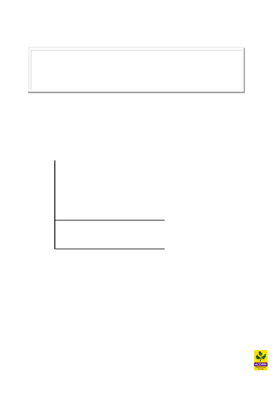
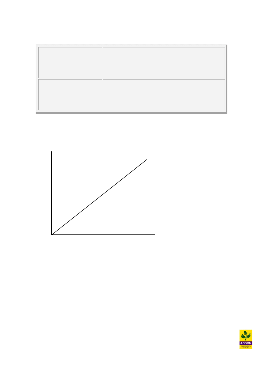
Indirect overhead or fixed cost is a cost which cannot be easily identified or related to a
cost per unit or activity of any kind e.g. a cost which remains constant when the production
of a good or service within the organisation rises or falls. Examples could include a factory
supervisor’s salary or factory rent and rates, or other non-production related expenses such as
the cost of running the marketing, finance or human resource department.
Fixed cost may also be referred to as a period cost e.g. incurred for an accounting period
regardless of sales or production levels. It is a cost that remains constant within certain limits
of an activity e.g. production or sales. The average fixed cost per unit (total fixed cost ÷ units
produced) would get smaller and smaller as production increases. This is because a constant
total fixed cost is being spread over more and more units produced, therefore the average
fixed cost per unit will fall as the production volume increases (vice versa).
The average variable cost per unit (total variable cost ÷ units produced) tends to remain
constant or does not change significantly as production increases. This is due to different
cost behaviour than fixed cost e.g. a variable cost is a constant amount incurred for each unit
produced.
Cost
(£)
Indirect overhead or fixed cost
Output or activity level (units)
5
1.4
Other types of cost behaviour
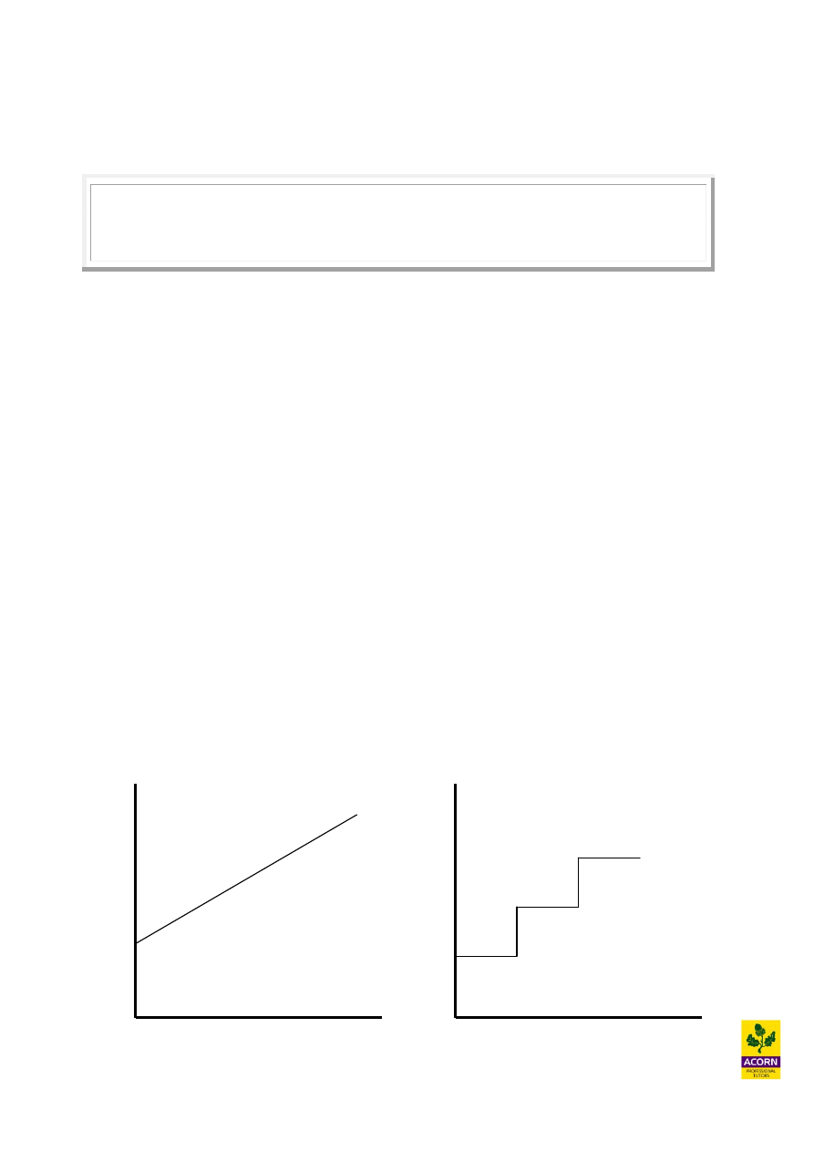
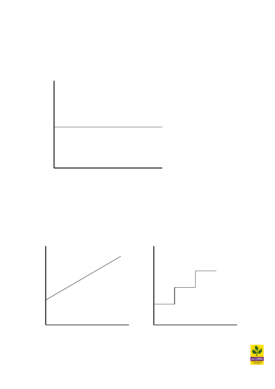
Semi-variable cost
A cost containing both fixed and variable components and thus partly affected by a
change in the level of activity. (CIMA)
A pure fixed cost remains constant when an activity level changes. A pure variable cost
would rise and fall directly (in a constant and linear manner) when an activity level changes.
The distinction is not always so clear cut in reality. A cost can be a mixture of both
variable cost and fixed cost and if so referred to as mixed cost, semi-fixed cost or semi-
variable cost e.g. a factory worker could be paid a fixed wage regardless of production (fixed
cost) but also an extra payment for each unit that person assembles or produces (variable
cost).
Stepped fixed cost
Fixed cost over the long-term will normally display the characteristics of ‘stepped’ cost
behaviour. That is the cost remains constant but only within a certain range of production.
Once this range of production is exceeded the fixed cost will rise.
Once a factory reaches full capacity extra leasehold expenses will need to be incurred to
obtain more buildings, if production is to increase or expand further. Therefore once a
certain range of production is exceeded, fixed cost will rise, but then remain constant over the
next range of output. Another example is supervisor’s salaries, they could be paid fixed
salaries, but supervision is limited to how many workers that can be supervised. Once the
size of the workforce exceeds a certain range another supervisor will need to be employed.
Most fixed cost generally displays the characteristics of stepped cost behaviour in the long-
term. In the long-term most fixed cost could actually be avoidable and is therefore variable
cost e.g. factory rent is fixed in the short to medium term, but could be avoided if the factory
were closed.
Example - Semi-variable cost
Example - Stepped fixed cost
Cost
Cost
(£) (£)
Activity level
Activity level

6
1.5
Forecasting techniques
Forecasting methods budget, forecast or project by extending historical data into the future,
the various techniques include.
High-low technique
The ‘line of best fit’ using human judgement
Regression analysis (or ‘least squares method’)
Time series
We will look at “high-low technique” and “line of best fit” in this chapter and “regression
analysis” and “time series” will be looked at in a later chapter.
If using historical information
1. Ensure a good time horizon in to the past; this is because we need to understand
seasonal, random or cyclical variations which may distort the overall trend.
2. Examine the information carefully to ensure it is complete accurate and valid.
3. Look at the methods of how it was collated and ensure it has not been contaminated.
All the above methods normally focus on creating a linear relationship for sales or cost
forecasting, normally expressed as;
Y= a + bX
Y = ‘the dependent variable’ e.g. total cost (or total sales)
X = ‘the independent variable’ e.g. an activity level driving total cost or sales
such as hours, units, time etc
a = ‘the fixed amount (constant) when X is zero’ e.g. fixed cost (or fixed sales)
b = ‘the gradient or the change in Y when X changes’ e.g. the variable cost (or
variable sales) driven by the activity level
Once a trend can be found by using the above methods, this linear forecasting function can be
used in order to forecast for other activity levels. Interpolation is when you are estimating an
activity within the given range of the data that you would have used to produce the trend
with. This is more likely to be accurate than ‘extrapolation’ techniques which is estimating
outside of the given range of data that you have.
Note: using historical information may not always be a good guidance for forecasting the
future.

7
1.6
High-low technique
A fixed (indirect) cost normally remains constant (in total) as the activity level changes. A
variable (direct) cost would normally rise or fall at a constant rate as the activity level
changes. A mixed or semi-variable cost containing both fixed and variable components
would only be partly affected by a change in the activity level.
With a mixed cost, as the activity level changes, the variable cost component would change,
however the fixed cost component would remain constant. The high-low method helps split a
semi-variable or mixed cost into its different fixed and variable components. Without doing
this it would be very hard to predict how a cost is likely to behave when a decision is made to
increase or decrease the activity. This may help assist with more effective budgeting or
forecasting for an organisation.
The high-low method uses the highest and lowest level of activity given (if more than two
activity levels are displayed within a question) and the associated costs, to separately identify
the variable and fixed cost components. The high-low method does this by recognising the
characteristics of variable and fixed cost behaviour. It works out the variable cost first and
then the fixed cost as a balancing figure. Such a technique could also be applied when you
have a mixture of fixed and variable sales and need to predict how this rises and falls with an
activity e.g. for different time periods.
The high-low method creates a linear (straight line) forecasting model expressed as;
Y = a + bX
Example 1.2 – Worked example
You are given the following cost information for a company that manufactures high quality
garden gnomes;
Units produced
Total cost (£)
12,000
53,000
14,000
59,500
16,000
66,000
Using the high-low technique estimate the cost of producing 10,000 units?
Step 1 Identify the variable cost
Compare the change in activity to the change in cost. Use only the highest and lowest
activities given and ignore all other activities given as data.
8
Units produced
Total cost (£)
16,000
66,000
12,000
53,000
4,000
13,000
£13,000 / 4,000 units = £3.25 direct cost per unit produced
Step 2 Identify the fixed cost as the balancing item
Use either 16,000 or 12,000 units above to work out fixed cost as the balancing figure.
TC = FC + (VC per unit x units produced)
66,000 = FC + (3.25 x 16,000)
66,000 = FC + 52,000
FC = 66,000 - 52,000
FC = 14,000
Forecast of total cost at 10,000 units
TC = 14,000 + (3.25 x units produced)
TC = 14,000 + (3.25 x 10,000)
TC = £46,500
Example 1.3 – (CIMA past exam question)
XYZ Ltd is preparing the production budget for the next period. The total costs of
production are a semi-variable cost. The following cost information has been collected in
connection with production:
Volume (units)
Cost
4,500
£29,000
6,500
£33,000
Calculate the estimated total production costs for a production volume of 5,750 units.
Advantages of the high-low technique
Easy method to calculate fixed and variable components from a mixed cost.
Easy method to learn and to understand.
9
Limitations of the high-low technique
Not very scientific as a method e.g. only uses two sets of data, not all the data
available, therefore reduces the potential accuracy of the forecasting model.
It uses the two most extreme ranges of data available e.g. the lowest and highest
values. These two ranges are generally the most inefficient for an organisation
therefore reducing the potential accuracy of the forecasting model.
It uses historical data as a basis of forecasting cost or sales e.g. past performance may
not be a good indicator or guide to the future.
It assumes the activity level is the sole driver of cost or sales, in reality many other
circumstances effect cost or sales not just activity levels e.g. labour efficiency levels
for cost or seasonality changes effecting sales.
Example 1.4
Tastes like can but boy does it sell Ltd, installs and fills up regularly canned vending
machines, selling a whole range of fizzy pop brands in restaurant, pubs and hotels. At
present it is trying to predict sales forecasts for some new vending machines being sold in
Spain and has obtained the following information from vending machines installed in other
Countries with similar climates.
Temperature (
0
Celsius)
Canned drinks sold per day
31 1,400
32
1,520
26
1,220
25
1,080
22
1,000
18 900
Create a forecasting model using the high-low technique and forecast the sales in units
for a temperature of 28
o
Celsius?
1.7
Scatter-graphs and ‘the line of best fit’
A scatter-graph is a graphical method of creating a forecasting model by using the ‘line of
best fit’ drawn free hand that closely matches or approximates to a series of data that has
been plotted on the graph. The line of best fit when drawn, tries to minimise the vertical
distance between all the data points plotted on the graph. The line of best fit can then be used
to predict the fixed and variable components for cost or sales, creating a linear (straight line)
forecasting model just like the high-low method.
10
The example below uses the information from example 1.4 to demonstrate how a scatter
graph can be used to create a forecasting model Y = a + bX.
Inspection
costs in £
1,000
2,000
3,000
100
200
300
400
Output in units
x
x
x x
x
x
Advantages of using scatter-graphs
Visual rather than calculative.
Easier to understand and interpret than the high-low method.
Uses all data available and plotted on a graph rather than just two sets of values in
contrast to the high-low method. Also with the high-low method the two sets of
data used are the most extreme of a given range and maybe unrepresentative of all
data given when used to create a forecasting model.
Limitations of using scatter-graphs
Not very scientific as a method e.g. uses a subjective ‘free hand’ line of best fit to
predict fixed (a) and variable (b) components.
It uses historical data as a basis of forecasting e.g. past performance may not be a
good guide or indication of the future.
It assumes the activity level is the sole driver of cost or sales, in reality many other
circumstances effect cost or sales not just activity levels.
Sales
units (Y)
2000
1000
Temperature (X)
10 20 30
Fixed sales (a) calculated
where the line of best fit
intersects the vertical axis.
Δ Sales (units)
Δ temperature
o
C
Variable sales (b) calculated by using the
gradient of the sales line e.g. the change (Δ) in
cans sold (ΔY) divided by the change (Δ) in
temperature as an activity (ΔX).

11
1.8
Classifying costs
Production expenses
Direct material e.g. the direct raw material or component cost of making the product.
Direct labour e.g. the labour physically engaged in making or assembling the product
such as basic wages or overtime paid to factory staff.
Variable production overhead e.g. direct factory expenses other than material or
labour such as hiring production equipment, fuel, power, heat, or consumables such as
grease/oil/cloths required for production.
Note: The total of direct material, direct labour and variable production overhead is referred
to as prime cost.
Fixed production overhead e.g. production overhead incurred not easily attributed or
ascertained to a cost object or cost unit e.g. factory supervisor salaries, factory rent
and rates, depreciation charges in the period for plant and machinery, the cost of
running the factory canteen, quality control department or inbound warehousing for
raw material and components.
Note: The distinction between variable and fixed production overhead is not always
definitive as often production overhead includes both a variable and fixed component.
Non-production overhead
Administration overhead (administrative direction and control over the organisation)
e.g. office salaries, office equipment, office heat and lighting, telephone, stationary
and insurance. The cost of running a purchase, finance, human resource or IT
department.
Selling overhead (promotion of the product and retention of customers) e.g.
advertising, cost of sales promotions, catalogues, brochures, salaries and commission
paid directly to sales staff. The cost of running a sales department or showroom.
Distribution overhead (packing and delivery of the product) e.g. cardboard, shrink
wrap and transportation cost such as the depreciation of vehicles, fuel or driver
salaries. The cost of packaging, outbound warehousing and transportation of finished
goods.
Note: The above non-production overheads can be variable, semi-variable or fixed.

12
1.9
Period and product costs
A period cost is a cost deducted as an expense during an accounting period; it is a cost
relating to time rather than the manufacturing or brought in cost of a product. Non-
production related expenses are examples of a period cost e.g. not ascertained to the cost of
making a product, instead written off in the period in which each expense is incurred.
A product cost is the cost of making a finished product or the cost of purchasing a product
for resale. Such costs are included in the value of inventory if the product is unsold at the end
of the financial period. The product cost of manufacture would include the prime cost e.g..
direct production cost of making the product. It is also normal for manufacturing
organisations to apportion an element of fixed production overhead to each unit made.
13
Key summary of chapter
Financial Accounting
(External information)
Financial accounts are produced mainly for external
users e.g. shareholders or investors.
Management Accounting
(Internal information)
Management accounts are produced for internal users
of financial information within an organisation e.g.
directors and management.
Types and classification of costs
A direct cost or variable cost is a cost that can be easily identified or related to a cost
per unit or activity level.
Cost
(£)
Direct or variable cost
Output or activity level (units)
14
Indirect overhead or fixed cost is a cost which cannot be easily identified or related
to a cost per unit or activity level. Examples include a factory supervisor’s salary or
factory rent and rates.
Semi-variable cost is a cost containing both fixed and variable components and thus
partly affected by a change in the level of activity.
Stepped fixed costs are fixed costs that remain constant but only within a certain
range of production. Once this range of production is exceeded the fixed cost will
rise.
Cost
(£)
Indirect overhead or fixed cost
Output or activity level (units)
Example - Semi-variable cost
Example - Stepped fixed cost
Cost
Cost
(£) (£)
Activity level
Activity level

15
Forecasting techniques
Forecasting methods budget, forecast or project by extending historical data into the future,
the various techniques include.
High-low technique
The ‘line of best fit’ using human judgement
Regression analysis (or ‘least squares method’)
Time series
The linear relationship for sales or cost forecasting, normally expressed as Y= a + bX
High-low technique
The high-low technique uses the highest and lowest level of activity given and the associated
costs, to separately identify the variable and fixed cost components.
The ‘line of best fit’ using human judgement
A scatter-graph is a graphical method of creating a forecasting model by using the ‘line of
best fit’ drawn free hand that closely matches or approximates to a series of data that has
been plotted on the graph.
Production expenses
Direct material e.g. the direct raw material
Direct labour e.g. the labour physically engaged in making the product such as
factory staff wages.
Variable production overhead e.g. direct factory expenses other than material or
labour such as hiring production equipment.
Prime cost = total direct material + total direct labour + total variable production
overhead
Fixed production overhead e.g. production overhead incurred not easily attributed or
ascertained to a cost object or cost unit e.g. factory supervisor salaries.
Non-production overhead
Those costs which are not directly relate to the making of the product but support this
process. For example administration overhead, selling overhead and distribution
overhead.
A period cost is a cost deducted as an expense during an accounting period; it is a cost
relating to time rather than the manufacturing or brought in cost of a product
A product cost is the cost of making a finished product or the cost of purchasing a product
for resale.

16
Solutions to lecture examples

17
Chapter 1
Example 1.1
A cost unit is a product, service or output of some kind in which costs can be ascertained, give
three examples of a cost per unit that could be used for a hospital?
Cost per treatment e.g. pharmaceuticals and staff time
Cost per bed per night for an inpatient
Cost per hour for different types of doctor or nurse
Example 1.3 – (CIMA past exam question)
Work out variable cost
Units
Overhead cost (£)
6,500 33,000
4,500 29,000
2,000 4,000
£4,000 / 2,000 = £2 variable cost per unit.
Work out fixed cost
Use either 6,500 or 4,500 units to work out the fixed cost as a balancing figure.
£29,000 = Fixed cost + (4,500 x £2)
£29,000 = Fixed cost + £9,000
Fixed cost = £20,000
Therefore
a = £20,000
b = £2
The budget for 5,750 units
Y = £20,000 + (£2 x 5,750)
Y = £31,500
18
Example 1.4
Step 1 Identify the variable sales
Compare the change in temperature to the change in sales. Use only the highest and lowest
temperatures given and ignore all other temperatures given as data.
Temperature (Celsius)
Canned drinks sold per day
32 1,520
18 900
14 620
620 / 14 = 44.28 cans sold per 1
o
Celsius.
Step 2 Identify the fixed sales as the balancing item
Use either 32
o
or 18
o
to calculate the fixed sales as the balancing figure.
1,520 = Fixed sales + (32 x 44.28 per 1
o
Celsius)
1,520 = Fixed sales + (1,417)
Fixed sales = 1,520 – 1,417
Fixed sales = 103
The forecast at a temperature of 28
o
Forecast = 103 + (44.28 x
o
Celsius)
103 + (28 x 44.28) = 1,343 canned drinks forecast to be sold
Wyszukiwarka
Podobne podstrony:
P1 Advanced mathematics for budgets
Types of A V Aids and relevance for LT
development of models of affinity and selectivity for indole ligands of cannabinoid CB1 and CB2 rece
Wicca Book of Spells and Witchcraft for Beginners The Guide of Shadows for Wiccans, Solitary Witche
Types of A V Aids and relevance for LT
Assessment of balance and risk for falls in a sample of community dwelling adults aged 65 and older
THE FATE OF EMPIRES and SEARCH FOR SURVIVAL by Sir John Glubb
Financial analysis of the cultivation of poplar and willow for bioenergy Belgia 2012
Initial Assessments of Safeguarding and Counterintelligence Postures for Classified National Securit
History of Jazz and Classical Music
Student Roles and Responsibilities for the Masters of Counsel
The problems in the?scription and classification of vovels
Legg Calve Perthes disease The prognostic significance of the subchondral fracture and a two group c
3 T Proton MRS Investigation of Glutamate and Glutamine in Adolescents at High Genetic Risk for Schi
(ebook pdf) Mathematics A Brief History Of Algebra And Computing
Best Available Techniques for the Surface Treatment of metals and plastics
więcej podobnych podstron