
A NEW METHODOLOGY FOR AUDIO FREQUENCY
POWER AMPLIFIER TESTING BASED ON PSYCHOACOUSTIC
DATA THAT BETTER CORRELATES WITH SOUND QUALITY
BY
Daniel H. Cheever
B.S.E.E. 1989, University of New Hampshire
THESIS
Submitted to the University of New Hampshire
in partial fulfillment of the Requirements for the Degree of
Master of Science
In
Electrical and Computer Engineering
December 2001

This Thesis has been examined and approved.
______________________________
Thesis Director, Prof. John R. Lacourse,
Chairman of the Electrical and Computer
Engineering Department
______________________________
K. Sivaprasad, Professor, Electrical and
Computer Engineering Department
______________________________
L.G. Kraft, Professor, Electrical and Computer
Engineering Department
______________________________
Date
ii

DEDICATION
I dedicate this thesis to my wife Sylvia, whom has given me the conviction
and support to succeed in whatever I attempt. I must emphasize that not all I have
attempted has been completed, though. My audio hobby has resulted in a basement full of
electronic scrap from many eras and quite homely hi-fi equipment in living areas in
various states of repair. I recall her asking about a certain MC head amp “why do you
need a pre-amp for your pre-amp”. Moreover she has had to put up with my near
religious following of rather nebulous aspects of sound reproduction.
Indeed I had promised her at the initiation of my graduate work in 1993
that I would be completed before our first born. Alexander is now 5 and Sophia 3. I thank
her for her patience while I “putzed around” in the basement bent on building better and
better amplifiers. I thank her for her help typing the thesis and all her efforts towards
revising some sections to be more readable and somewhat more earthbound.
iii

TABLE OF CONTENTS
DEDICATION………………………………………………………………….…..
iii
LIST OF TABLES……………………….………………………………………….
vi
LIST OF FIGURES……………………….………………………………………...
vii
ABSTRACT…………………………………………………………………………
ix
CHAPTER
PAGE
INTRODUCTION…………………………………………………………………..
1
I. The lack of correlation between objective measurements and subjective sound
quality- history and examples……………………………………………………..
2
1. Introduction…………………………………………………………...…….
2
2. The history of audio measurements …………………...…………..….…....
5
3. Examples of standard measurements ……………………….……...……....
21
4. Conclusion- a call for a new methodology……………………...…….…....
31
II. A new audio test philosophy……………………………………………………..
34
1. Harmonic consonance.………..……………………..………...……....……
35
2. The sound pressure level dependence of the aural harmonic
envelope……………………………………………………………………….
41
3. Intermodulation distortion.………………..…..…………..…………...……
49
4. Pre-transient noise bursts.………………..…..……....…………….....……
51
5. The fallacy of negative feedback as a cure-all……………………………...
52
III. Measurement protocol of the Total Aural Disconsonance figure of merit……...
64
1. Device measurements……………………………………………………...
64
2. A measurement protocol for the Total Aural Disconsonance figure of
merit………………………………………………………………………..
68
IV. Conclusion………………………………………………………...…………….
72
Bibliography………………………………………………..……………………….
v
76

LIST OF TABLES
Table 1-1
Comparison between distortion mechanism and
measurement type
Pg. 18
Table 2-1
Spreadsheet based T.A.D calculations for two amplifiers.
Pg 47
Table 2-2
Distortion components versus feedback level for a square
law dominated gain device
Pgs. 56-57
Table 2-3
Distortion components versus feedback level for an
exponentially non-linear gain device.
Pg. 61
Table 3-1
Aural Harmonics from Eq. 2-1 over a reduced S.P.L range.
Pg. 58
vi

LIST OF FIGURES
Fig. 1-1
Poor standard test measurements for an excellent sounding
amplifier
Pg. 3
Fig. 1-2
Standard measurements for a modern amplifier with average
sound quality
Pg. 4
Fig. 1-3
Correlation between different harmonic order weighting and
subjective sound quality
Pg. 9
Fig. 1-4
Overload characteristics “hidden” inside the feedback loop
Pg. 12
Fig. 1-5
Disagreement between clipping distortion measurements
between the common average reading meter and peak
harmonic percentage.
Pg. 13
Fig. 1-6
Comparison of Dynamic I.M. with common I.M.D
Pg. 17
Fig. 1-7
FASTtest Methodology and spectrum
Pg. 17
Fig. 1-8
Performance comparison between FASTtest and other
methods.
Pg. 20
Fig. 1-9
Hafler DH500 audio power amplifier schematic, one channel
shown.
Pg. 21
Fig. 1-10
Block diagram of test set-up.
Pg. 23
Fig 1-11
DH500 distortion components and T.H.D at 1 kHz, 32W.
Pg. 24
Fig. 1-12
DH500 distortion components and T.H.D at 15 kHz, 23W
Pg. 24
Fig. 1-13
DH500 intermodulation distortion, 4kHz:15kHz at 4W.
Pg. 25
Fig. 1-14
DH500 D.I.M, 3.18kHz:15kHz, 10W
Pg. 26
Fig. 1-15
Schematic of the type 45 triode tube based Single-ended audio
amplifier
Pg. 28
Fig. 1-16
Type 45 S.E. amplifier frequency response
Pg. 28
Fig. 1-17
Type 45 S.E. amplifier 1kHz harmonic distortion components
at 0.4W
Pg. 29
Fig. 1-18
Type 45 S.E. amplifier 200Hz-7kHz IM
Pg. 29
Fig. 1-19
Type 45 S.E. amplifier 14kHz:15kHz IM
Pg. 30
Fig. 1-20
Type 45 S.E. amplifier D.I.M
Pg. 30
Fig. 2.1
Ear self-generated harmonics, frequency versus level.
Pg. 36
Fig. 2-2
Ear self-generated harmonics, level versus sound pressure
level
Pg. 37
Fig. 2-3
Ear self-generated harmonics, level versus sound pressure
level
Pg. 37
Fig. 2-4
Subset of Fig. 2-3 with reduced SPL range for clarity
Pg. 38
Fig. 2-5
Pitch change necessary to distinguish a second tone
Pg. 39
Fig. 2-6
Tone masking research showing aural harmonics
Pg. 40
Fig. 2-7
Showing fit of Eq. 2.1 versus Olson aural harmonic test data.
Pg. 42
Fig. 2-8
1.5W Type 45 triode feedback-less single-ended amplifier at
0.32 W rms.
Pg. 46
Fig. 2-9
10W Bi-polar transistor feedback amplifier at 0.72 W rms.
Pg. 46
vii

Fig. 2-10
Two amplifiers distortion harmonics versus aural harmonics.
Pg. 47
Fig 2-11
D.I.M. measurement example for a non-feedback amplifier
Pg. 50
Fig. 2-12
D.I.M. measurement example for a feedback amplifier
Pg. 50
Fig. 2-13
Negative feedback block diagram
Pg. 52
Fig. 2-14
Transconductance graph for a power field effect transistor
Pg. 55
Fig. 2-15
Calculated distortion versus feedback level using the equations
in table 2-2.
Pg. 58
Fig. 2-16
Calculated distortion versus feedback level using the equations
in table 2-3.
Pg. 62
Fig. 3-1
Schematic of the single-ended F.E.T. output stage.
Pg. 64
Fig. 3-2
Calculated and measured distortion versus feedback level, FET
SE output stage.
Pg. 66
Fig. 3-3
Subset of the DH500 amplifier schematic showing the point
where feedback is removed and a signal injected.
Pg. 69
Fig. 3-4
DH500 Open-loop harmonic distortion at 0.4W
Pg. 70
Fig. 3-5
Output level variation of the type 45 SE amplifier when loaded
with a loudspeaker
Pg. 74
viii

ABSTRACT
A NEW METHODOLOGY FOR AUDIO FREQUENCY
POWER AMPLIFIER TESTING BASED ON PSYCHO-ACOUSTIC
DATA THAT BETTER CORRELATES WITH SOUND QUALITY.
By
Daniel H. Cheever
University of New Hampshire, December 2001
There exists general agreement that the commonly accepted test and
measurement protocols for audio frequency power amplifiers fail to correlate with the
subjectively accessed devices sound quality. A review of the history of audio testing was
undertaken to reveal if prior art has produced tests that better correlate with sound
quality. A universal concept emerged, one that calls for stronger weight of the higher
order, more aurally discordant harmonic distortion products, over the low order, more
benign harmonics. Separately a study of the psychoacoustics of the ear resulted in a
mathematical derivation of the ears intrinsic aural distortion. The two are combined and
offer a methodology for weighing the harmonics based on a dimensionless figure of merit
that quantifies the amplifier’s harmonic distortion envelopes departure from the ears aural
masking, named Total Aural Disconsonance or T.A.D. It is shown both analytically and
through actual device measurements that the application of negative feedback, regardless
of level, results in poorer T.A.D. figures. Two amplifiers of opposing standard
measurement results are fully tested and subjectively analyzed and results show that the
T.A.D. method outperforms classic T.H.D and I.M. for characterizing amplifier quality.
ix

1
INTRODUCTION
Humans respond emotionally to complex musical messages that contain no real
survival value. This phenomenon indicates that the human brain is instinctively motivated
to entertain itself with sound processing primary sense operations. This is a cross cultural
phenomenon that most likely results from an inborn drive to learn, at an early age, the
sophisticated auditory analysis required for speech perception. Aesthetic appreciation of
music may be due to man’s need to exercise their neural network.
In this era we have access to musical reproduction equipment in a range of
qualities. High fidelity equipment strives to reproduce the original musical event. Perfect
fidelity is perfect reproduction of the signal. A modern music reproduction system relies
on recorded music being reproduced via sound transducers. Microphones convert the
instantaneous acoustic pressure of the musical performance into electrical signals. These
signals are amplified and recorded onto media. The playback devices output is amplified
by an audio power amplifier which drives the loudspeakers. On all the elements in the
chain, except for the power amplifier, there is general agreement between the current
standardized fidelity objective specifications and the sound quality. This thesis is an
investigation of the hypothesis that the current accepted measurements that quantify
fidelity of an amplifier fail to correlate well with subjective sound quality. Proposed is a
more accurate set of measurement protocols.

2
CHAPTER 1
THE LACK OF CORRELATION BETWEEN OBJECTIVE MEASUREMENTS AND
SUBJECTIVE SOUND QUALITY- HISTORY AND EXAMPLES.
1. Introduction
In September on 1995, Stereophile, an established highly respected hi-fi
magazine, ran a review of the Cary 300SEI,
the first mainstream review of a single ended
amplifier
1
. In this design, a single output device is tasked with producing both polarities
of the signal swing and had zero negative feedback. Robert Hartley, one of the senior
reviewers, states:
The 300SEI communicated music in a way I’d never experienced before. There
was an immediacy and palpability to the sound that was breathtaking- a musical
immediacy the riveted my attention to the music. It reproduced massed violins
with beauty unmatched by any electronics I’ve had in my system. It excelled in
the most important areas: Harmonic rightness, total lack of grain, astonishing
transparency, lifelike sound staging, and a palpability that made the instruments
and voices exist in the room.
[2]
The article then follows with the standard lab bench test results such as harmonic
distortion spectra, frequency flatness, etc. Every specification; output power, frequency
1
Stereophile Magazine
[1]
. September 1995 pp.141-149.
3
response, output impedance, harmonic distortion, and intermodulation distortion, were
the poorest results I have noted published.
This amplifier measured so poorly as to be a joke…contrary to what we consider
good technical performance. I’m convinced the 300SEI doesn’t harm the signal
in ways push-pull amplifiers do, and that what the 300SEI does right is beyond
the ability of today’s traditional measurements to quantify. I have become
convinced single ended tube amplifiers sound fabulous in spite of their distortion,
not because of it.
[3]
Fig. 1-1
[4]
Poor standard test measurements for an excellent sounding amplifier
4
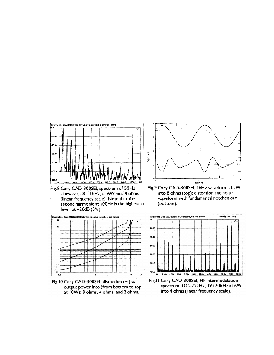
Figure 1-1 speaks for the obvious concern that the objective measurements of this
amplifier are very poor. Compare the results in Fig. 1-1 with the following Fig. 1-2 from
Fig. 1-2
[6]
Standard measurements for a modern amplifier with average sound quality

5
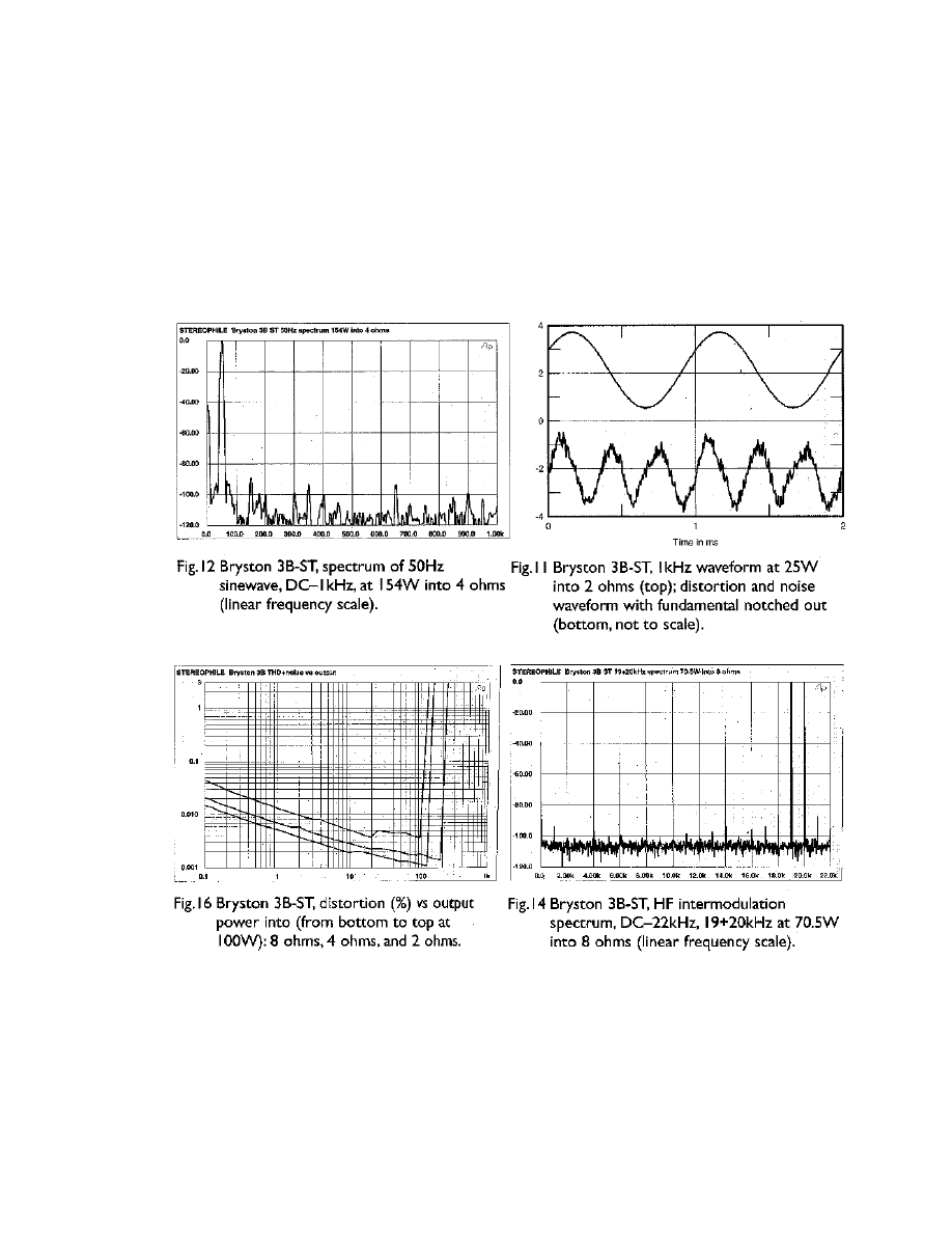
a renowned solid-state audio power amplifier, the 120 Watt per channel Bryston 3B-ST.
Note the harmonic distortion is nearly 100dB down, over 7000 times “better” than the
Cary CAD-300SEI. Intermodulation distortion 85dB down, or 500 times “better”.
Distortion only 0.002% at 100W compared to over 2% at 8W for the Cary CAD-300SEI.
Yet, the review of the Bryston 3B-ST resulted in comments on lack of smoothness and
high frequency transparency, and of other amplifiers offering better imaging and
transparency. This same language was used in the review of the Cary CAD-300SEI, and
precisely in the areas where the CAD-300SEI excelled. These trade magazines are a
common way the buying public informs itself on sound reproduction equipment buying
decisions. Indeed there exist F.T.C.
2
regulations on the publishing of common amplifier
measurement results. The purpose of this thesis is to investigate if there are measurement
parameters that have been overlooked, avoided, or conveniently been ignored in the
reproduction of quality sound for human enjoyment
2. The History of Audio Measurements.
Since the review of the Cary CAD-300SEI almost no issue of an audio
publication
3
has been without a glorious review of a simple topology amplifier followed
by atrocious technical measurements. An in depth historical study was undertaken to
2
Federal Trade Commission. For example the text on the shipping carton of an amplifier “80 watts per
channel at 0.08% THD over 20-20kHz” requires the following of the F.T.C. test guidelines.
3
I have a large private collection of audio magazines. Including Stereophile 1988 – present, Stereo Review
1982-1987, Listener 1991- present, Audio 1982 – 1989.

6
investigate possible existing but not popularized testing methodologies that may
correlate better with audio quality perception.
In 1925 Edward Kellogg, the co-inventor of the moving coil loud speaker,
wrote a landmark paper “The design of non-distorting power amplifiers”
[6]
. It suggests
that 5% distortion is the permissible limit for audio amplifiers.
He indicated that this
much distortion can be tolerated only when the curvature of the transfer characteristic is
“uniform” rather than “turning abruptly”. This is the first implication that amplifier
quality is diminished if the distortion products are not of low order. Kellogg and others
at this time measured distortion by inserting a notch filter at the fundamental and reading
the value of any remaining harmonics and noise on an AC voltmeter. Today this is the
most common specification used called total harmonic distortion (T.H.D.
4
). The triode,
the only amplifying device available at that time, when used correctly, keeps the
harmonic order of the distortion to the first two harmonics thus there is good correlation
with sound quality in quoting simple percentage figures. The commercial focus since
then seems to be on reducing the commonly measurable aspects of harmonic distortion
without regard to the non-linearity of amplification devices.
The origin of the era of correlating amplifier quality with distortion
measurements begins with a statement by W.T. Cocking in 1934
[7]
. He suggested that
4
Commonly T.H.D. or Total Harmonic Distortion, is actually the Root Mean Square sum of the harmonics
in the audible frequency range of a mid-band test signal. The individual harmonic powers are squared,
added together, and the square root results in the T.H.D. figure.

7
5% distortion was too high for quality amplification. Cocking compared triodes to the
newly released pentodes and found triodes preferable due to the less objectionable
distortion products and its ability to better damp the loudspeaker. That same year Harold
S. Black published “Stabilized Feedback Amplifiers”
[8]
. Black conceptualized negative
feedback. He found that by returning to the input an inverted portion of the output signal
distortion was reduced by the same ratio as gain. Negative feedback was now without
exception implemented in all power amplifier designs. Quickly class AB
5
push-pull
design with more efficient pentodes became more popular with higher power output and
lower cost than the triode based circuits. Three very successful examples are the 1945
Quad
[9]
(the Williamson), the 1949 McIntosh, 50W-1
[10]
and the 1951 Hafler Ultra-Linear
circuit
[11]
. All of these designs added circuit and output transformer complexity to allow
for use of the more non-linear pentodes. It is my opinion that the emerging trend was to
convince the consumers blind faith in specifications - maximize power and minimize
T.H.D.
Two papers in this period called to question the now standard T.H.D.
specification. The first was the 1937 Radio Manufacturers Association
6
“Specification
for amplifiers with two testing and expressing overall performance of radio broadcast
5
Class AB signifies a push-pull operating mode in where either device does not linearly amplify the entire
waveform. More plainly stated, the opposing polarities of the waveform are handed off between two uni-
polar devices with usually less than 5% overlap. The less overlap the more crossover distortion due to the
(all) devices transconductance being less linear near cut-off. More feedback thus is required to attempt
eliminate the crossover distortion.
6
U.K.

8
receivers”
[12]
. According to this procedure, when performing the sum of the individual
harmonics, the amplitude of the n
th
harmonic is multiplied by n/2. The contribution of
second harmonic is thus unchanged but higher harmonics are more and more severely
weighted due to the general agreement that higher order harmonics are more offensive to
the ear. No reference is sited on the sex, age, or the number of listeners. The state of the
art at this time includes push-pull amplifiers with feedback applied with varying levels of
subjective success. The originator of the RMA specification later writes that the
audibility threshold of the sample group was 5% second harmonic and 0.1% ninth
harmonic. “No simple x*n
2
weighing system was really correct.”
[13]
A stronger work was in 1950 by D.E.L. Shorter from the BBC engineering
research department “The influence of high order products in non-linear distortion”
[14]
.
“The commonly accepted figures for the maximum allowable non-linear
distortion in reproducing systems are based on work carried out many years
ago. Since then, new kinds of apparatus producing forms of distortion not
covered by early experiments have come into use, with the result that the
subjective assessments of non-linear distortions does not always agree with
the assessment based on measurement."
[14]
He shows the extent of the error that results from the practice of taking the R.M.S. Total
Harmonic Distortion as a criterion for subjective quality. He used a test program of solo
piano with microphone feeds through a selection of six audio power amplifiers having
high levels of negative feedback. The results are shown in Fig. 1-3. The upper two data
curves clearly show better agreement between measured distortion and the subjective
appraisal than the lower data for the common T.H.D R.M.S. sum of harmonics. The n/2
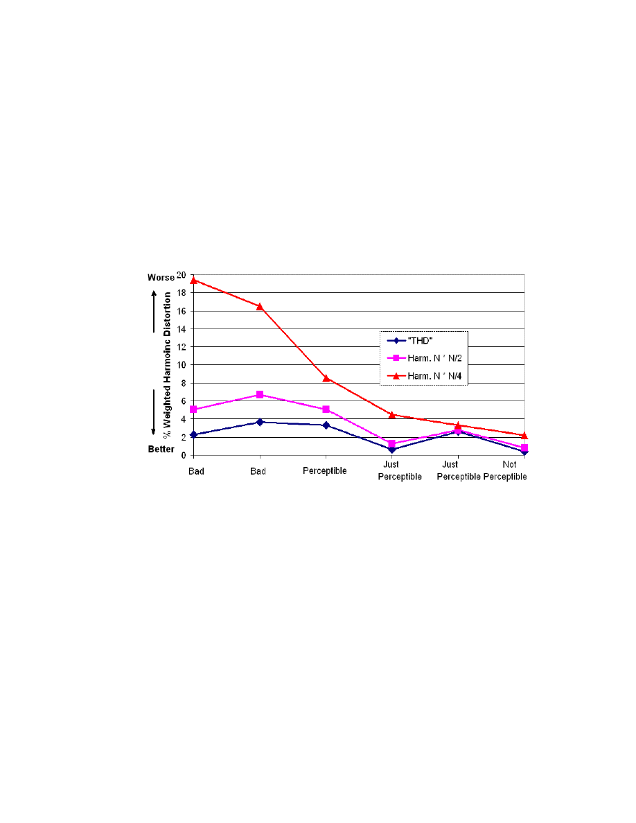
9
data is the weighting proposed by the R.M.A. The upper data has a more drastic
weighting of n
2
/4 and results in the best agreement between the merit figure and the
subjective appraisal as only this n
2
/4 data correlates correctly between the left most “bad”
amplifier and the “perceptible” amplifier. Although unsaid Shorter is inferring that the
“new types of equipment” meaning the feedback pentode designs, do not equal the
Fig. 1-3. Correlation between different harmonic order weighting
and subjective sound quality
subjective quality of equipment free from high order harmonics at a equal or even lower
measured distortion using today’s equal weighing method. This paper is also important
as it is the first to indicate that amplifiers producing high order harmonics from a single
tone will also produce a large number of intermodulation products when several tones are
applied. He calls for objective tests to be “so framed that they give the appropriate
numerical expression” for intermodulation distortion (I.M.D.). This is also the first

10
mention of the need to weight the I.M. products in rising order. The modern S.M.P.T.E
7
I.M. standard does not weight I.M. products.
Alan Bloch in 1953
[15]
mathematically shows that the THD and
heterodyne methods need corrected harmonic ratios due to the need to measure out-of-
band harmonics but that the new SMPTE intermodulation method
[16]
has the additional
advantage that the I.M. products are symmetrical around the test frequencies so that the
side band in the pass band can be used for test signals near the response extremes.
He
comments that the mathematical model does not have provision for weighting the higher
order terms. The problem is “should the distortion [individual harmonics] component
level be determined in order to obtain the best listener index?”.
Norman Crowhearst is the most prolific writer on audio technology in the
late 1950’s through the mid 1970’s. He is the lone technical voice in this period
campaigning for the concept that simply performing the standard SMPTE IMD or THD
test with better and better accuracy is not improving the selectivity of which amplifiers
sound better. Amplifiers at this time offer specifications of 0.05% THD and frequency
response within 0.1dB to hundreds of kHz. He states “By these figures such amplifiers
should sound the same and perfect”
[17]
. Crowhearst is first to propose that the very high
orders of harmonics due to the proliferation of high levels and multiple loops of feedback
create a signal correlated modulating noise floor. Static single sine test signal
7
Society for Motion Picture and Television Engineers

11
performance may not quantify this abrasive effect. In 1957 with “Some Defects in
Amplifier Performance not covered by Standard Specifications”
[17]
he explains that if the
feedback is accomplished in smaller loops
8
the frequency multiplying effect is further
aggravated, as the local loop will result in reduced 2
nd
and 3
rd
order harmonics and
generate small components of 4
th
through 9
th
. Then the global loop takes this and adds
further 4
th
, 6
th
, and due to the residual of the original 2
nd
and 3
rd
now contributes 8
th
, 12
th
,
16
th
, 18
th
, 24
th
, 36
th
, 54
th
and all the way to 81
st
! Any phase errors due to reactive loading
can accentuate rather than minimize high order harmonics. Crowhearst also shows that
the relationship between harmonic and IM measurement is not simple as he shows by
experiment. He is also first to bring light to the negative effects of the phase
compensating capacitor in the feedback loop, invariable used at this era for ensuring
stability in mid to high feedback amplifier designs. He graphically shows how if the
output presents a clean square wave response the amplifier relies on a high frequency
peak that is critically tuned in order for the feedback to null the ringing. Transient
response of the amplifier is marred as the transient performance into a reactive load is
worse than if no “trickery” was designed in. Much later work by M. Otala defines the
very high slew rate capability that the driver stages need in order to eliminate this effect.
Crowhearst eloquently details feedback amplifier overload characteristics that are hidden
8
As remains current practice, mainly because modern semiconductor f
t
is higher, so more feedback can be
applied locally to individual gain stages to linearize them and maintain stability. Almost all modern
amplifiers use both local and global negative feedback.
12
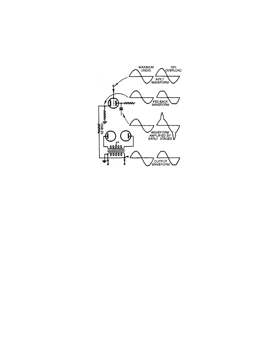
in standard tests. In reference to Fig. 1-4 he explains that when clipping starts the
Fig. 1-4. Overload characteristics “hidden” inside the feedback loop.
[17]
voltage is clipped so the waveform amplified by feedback summing node stages develops
a sudden peak – the difference between the input and the clipped output. This
progressively exaggerates the drive to the output and further increases the clipping. He
states
“This explains the familiar complaint that a certain 15 Watt amplifier seems to
give more clean output than a certain 60 Watt one…since if the input to the 60 W one is
exceeded at all it triggers into this severe distortion condition, distorting not only the peak
that caused it but also some of the program that follows”
In later papers such as the 1959 “Feedback – Head Cook and Bottle Washer”
[18]
Crowhearst shows how zero IM distortion can be faked by picking test frequencies that
13
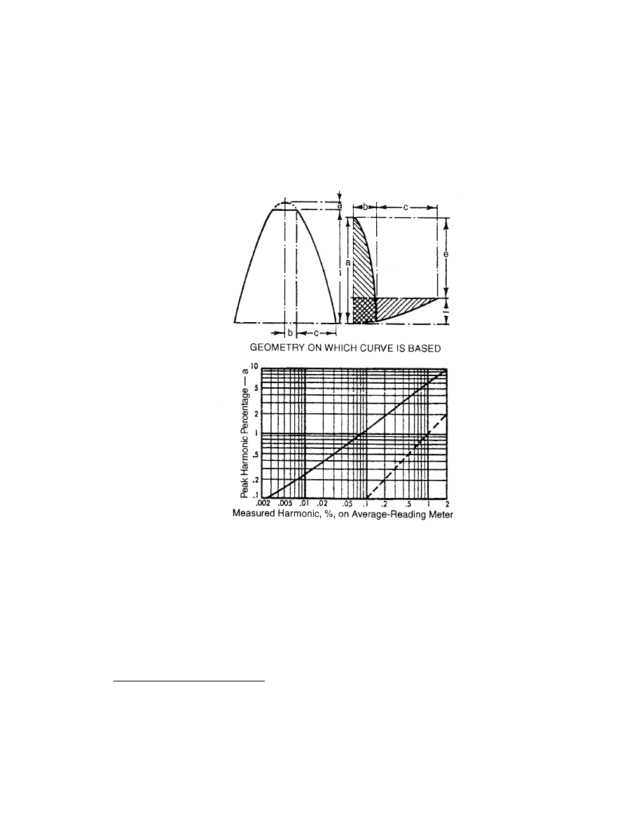
will null IM. He is also first to point out the miss-use of average reading meter to
measure THD at near clipping levels, as is necessary in the common distortion versus
Fig 1-5. Disagreement between clipping distortion measurements
between the common average reading meter and peak harmonic percentage.
output power graph. This is cleverly shown graphically in Fig 1-5. For example if the
input level exceeds the clipping level by 10% measured with an averaging harmonic
meter
9
over a complete cycle, the reading would be only about 2% but the effect is very
9
The prevalent instrument of the time. This was essentially a rectified and amplified signal that is
integrated by the mechanical meter element. The fundamental is notched out with a steep filter.

14
audible. Comparison with a similar size amplifier that clips less abruptly (yet earlier) but
with low order harmonics
10
would give incorrect conclusions as the distortion will
measure five (5) times higher (average) yet still be audibly benign. This peak to average
ratio measurement error is even more aggravated for high frequency IMD tests.
Crowhearst’s conclusions are similar to his predecessors in that distortion analysis be
based more on the transfer function linearity rather than on normal harmonic or IMD
statements. He further recommends that a standard real-world reactive load be agreed to
further test for stability and other distortions. He recommends rating amplifier power at
the point where the amplifier returns to linearity after overload, not at the point just
before. This is significant as he states that this latch up could account for up to 50% of
the audio power
11 , [18]
.
There follows a period until the mid 1970’s where there was little new
material criticizing conventional amplifier distortion measurements. The transistor was
virtually displaced by the vacuum tube in all audio circuits. The new transistor amplifiers
offer better specifications, wider frequency response, lower damping factors
12
, much
10
The specmanship race rears its ugly head throughout the history of audio amplification. As higher power
density output devices (lower cost per watt) became available they where used, but always they where less
linear, so more negative feedback would be required to “out-spec” the older design. The more feedback, the
sharper the onset of clipping, and the more abrupt the high-order audible distortions are introduced to the
output signal. I show in Chapter 2, Section 5 that the increase of high-order harmonics can be tolerated as
long as they follow a certain defined rate of increase.
11
1960’s era commercial pre-transistor audio power amplifiers
12
A measure of the output impedance of an amplifier. A damping factor of 2 means an output impedance of
equal to the loudspeakers nominal but while being a ideal power efficiency match this is considered very
poor as common loudspeakers impedance variations will cause frequency response aberrations. DF = Vno
load/(Vno load-Vloaded)

15
higher power versus production cost, and an order of magnitude lower T.H.D. than tube
based amplifiers. During this period low efficiency acoustic-reflex loudspeakers became
popular due mainly to their smaller size for the same subjective low frequency output.
The decrease in efficiency of these designs was substantial, requiring 4 to 10 times more
amplifier power. Additionally the impedance variations with frequency due to the under-
damped woofers reactance are far more substantial than the older, large designs. These
last two effects compound to make vacuum tube designs less attractive. In the popular
press at the time the new amplifiers etch and glare where educated to the consumer as
“detail”. These early amplifier designs are now universally considered un-listenable. An
example is the resale value and current regard of the two most popular amplifiers of all
time, the 1958 - 1990 Dynaco ST70 35W ultra-linear push-pull vacuum tube amplifiers
and the later solid state brother, the Dynaco ST120. The ST70 can fetch up to $500 on
resale with an incomplete parts only chassis never less than $200. I’ve noticed two
separate transactions on Ebay where the ST120’s sell for less than $20. Indeed the latest
issue of Listener magazine proclaims the Stereo 120 “the worst sounding amplifier ever
made”
[19]
while the ST70 reviewed the “Classics” column “giving me some of the best-
reproduced sound I have ever heard”. Why the discrepancy? It is now generally agreed
that the early solid state circuits had insufficient slew rate in the driver sections for the
large amount of negative feedback creating dynamic intermodulation distortions. The
first work on analyzing this behavior was in 1970’s “Transient Distortion in Transistor

16
Audio Power Amplifiers”
[20]
by Matti Otala, followed by “Circuit Design Modifications
for Minimizing Transient Intermodulation Distortion in Transistor Audio Power
Amplifiers”
[21]
He clearly shows how the slew rate of the front end gain stages and the
feedback network must exceed the signal bandwidth by a factor related to the amount of
negative feedback, at least 50 times for common applications. If this specification is not
met dynamic intermodulation distortion is created. His work is universally embraced and
founded the ultra-high bandwidth audio design era. In “A Method for Measuring
T.I.M.”
[22]
he proposed a method that yields quantitative measurements of dynamic
intermodulation distortion without the knowledge of the out-of-band behavior of the test
amplifier. He explains the use of a 15kHz sine wave and a 3.18kHz (low pass filtered at
15kHz) square wave. Total intermodulation distortion is given by Eq. 1-1. To
[
]
2
2
/
1
9
1
2
100
(%)
V
V
IM
n
nt
∑
=
=
Eq.1-1 where
V
nt
= peak amplitude of component f
2
– nf
1
V
2
= peak amplitude of test sinusoid.
determine dynamic intermodulation distortion (D.I.M.) the 3.18kHz filtered square wave
is used. Using a 3.18 kHz triangle wave instead results in S.M.P.T.E. I.M.D. T.I.M is
then calculated via T.I.M. = D.I.M. – I.M.D. Otala presents objective tests on eight audio
power amplifiers and most show T.I.M onset earlier and far more severe slope than the
17
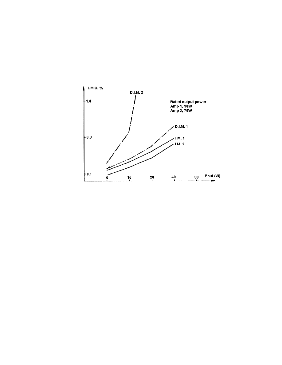
common the SMPTE I.M.D, reproduced in Fig. 1-6. His conclusion, documented by the
far earlier onset of T.I.M, is that the minimum slew rates for closed loop op-amp circuits
Fig. 1-6 Comparison of Dynamic I.M. with common I.M.D.
[22]
with 30kHz bandwidth be 10V/µs, and 100V/µs for power amplifiers. He states “These
results show that even the fastest present amplifiers must remain suspect as far as T.I.M
is concerned”
[22 pp. 175]
. Inspecting the D.I.M versus I.M. family for the two amplifiers in
Fig. 1-6 does show that I.M is an insufficient measure. Note amplifier no. 1, a 30W
model, the D.I.M tracks with I.M, but for no. 2, a 70W model D.I.M. departs from I.M
rapidly at less that ½ rated power. “The T.H.D and SMPTE-IM test methods give very
low distortion figures, even when the quality of the amplifier as judges with other tests is
completely unacceptable.”
[22 pp. 175]
.

18
One of Matti Otala’s later papers for the Journal of the Audio Engineering
Society is 1978’s “Correlation Audio Distortion Measurements”
[23]
. Here he combines a 2
stage op-amp circuit with non-linear feedback elements to create the common amplifier
distortion mechanisms. The conclusion table is presented below as Table 1-1. The THD
Distortion
Mechanism
THD
SMPTE-
IM
CCIF-IM
DIM
NOISE
Symmetrical
Output Non-linearity
Poor(1)
Good(10)
Excellent
Good
Moderate
Poor
Asymmetrical
Output Non-linearity
Poor(1)
Good(10)
Excellent
Poor
Excellent
Poor
Crossover Distortion
Poor(1)
Excellent
(10)
Excellent
Excellent
Poor
Poor
Hard Input-Stage
Limiting
zero
zero
Poor
Excellent
Excellent
Smooth Input Stage
Limiting
Zero(1)
Poor(10)
zero
Good
Excellent
Excellent
Table 1-1 Comparison between distortion mechanism and measurement type
(1) and (10) indicate the total harmonic distortion at 1 kHz and 10 kHz respectively.
SMPTE is total static 2 tone I.M. using the standard 7 kHz:200 Hz at 1:4 weighting.
CCIF is I.M. sub harmonics of two tones at 14 kHz and 15 kHz. The NOISE test is
performed by injecting band limited white, high-pass filtered at 48dB/oct. below 11 kHz.
Noise spectral density is measured with a spectrum analyzer in the frequency range of 0-
9kHz. Inspection of this comparison table reveals that no single listed amplifier testing
method successfully measures all the discussed distortions. The NOISE and DIM tests
are not commonly published on modern commercial equipment reviews. Input stage
limiting performance remains an untested parameter.
19
For the period of the late 1970’s on the audio testing literature concentrated
on advances in testing resolution using the existing standard measurements previously
discussed. The mid 80’s brought both digital audio and one-box automated testing
systems. Products such as the Audio Precision 1.0 became widespread, these used the
graphical interface provided by the personal computer and provided quick tests with great
repeatability but necessarily excluding any tests other than the common set available at
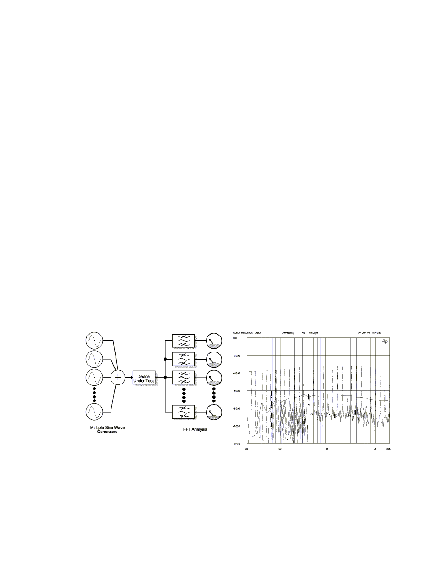
the top-level software control. Notable during this period is a development by Richard
Cabot, VP of Audio Precision of a complex test using multiple tones with distortion
calculated as the summation of the power of signals not at the injected frequencies. The
paper “Comparison of Nonlinear Distortion Measurement Methods”
[24]
introduces this
method called the FASTtest. In the paper he uses 59 individual tones, as shown and
described in Fig. 1-7. Non-linear components plus noise are detected and their value is
Fig 1-7. FASTtest Methodology and spectrum
[24]
20
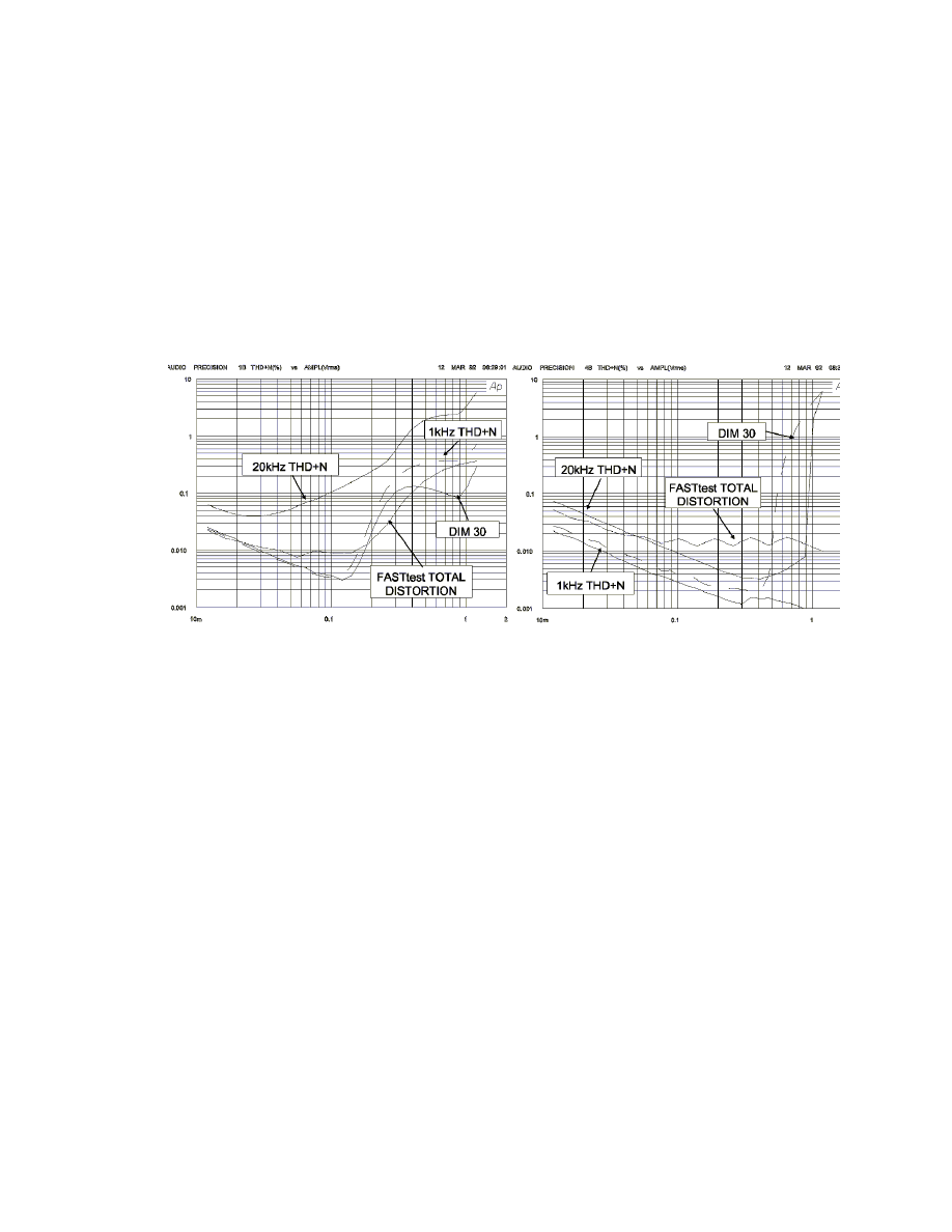
shown as the horizontal line in the right hand plot of Fig. 1-7. The performance of the
FASTtest in comparison with the common tests is shown in Fig. 1-8. The left-hand plot is
a simulation of harmonic distortion arising from output stage non-symmetry. The right
hand plot is slew rate limiting. In general the curves follow the same family of behavior
Fig 1-8 Performance comparison between FASTtest and other methods.
[22]
with no test method discernable as universally superior. Richard Cabot discusses the
ability of the system to weight the test signal amplitudes to better match the frequency
content of a musical signal. He does not mention any means for weighting the harmonic
components order, presumably as the system does not attempt to calculate the harmonic
products of each tone, but is rather an summation envelope of all tones harmonics. As
will be shown in the following sections of this paper the FASTtest methodology will not
produce measurements that better correlate with subjective quality than previous existing
methods.
21
3. Examples of standard measurements
This thesis work encompasses many years of measurements on different
amplifiers of differing designs. Presented is a full detailed analysis of two. The first is a
Hafler DH500, a well-respected commercial high power push-pull amplifier using
paralleled banks of MOSFET output transistors. The Hafler adequately represents the
current state of the art. It is rated at .02% THD from 20-20kHz at 255 Watts per channel.
The circuit is a typical modern no frills design of the philosophy that a simple signal path
gives the best results. The feedback is single pole passively compensated via the
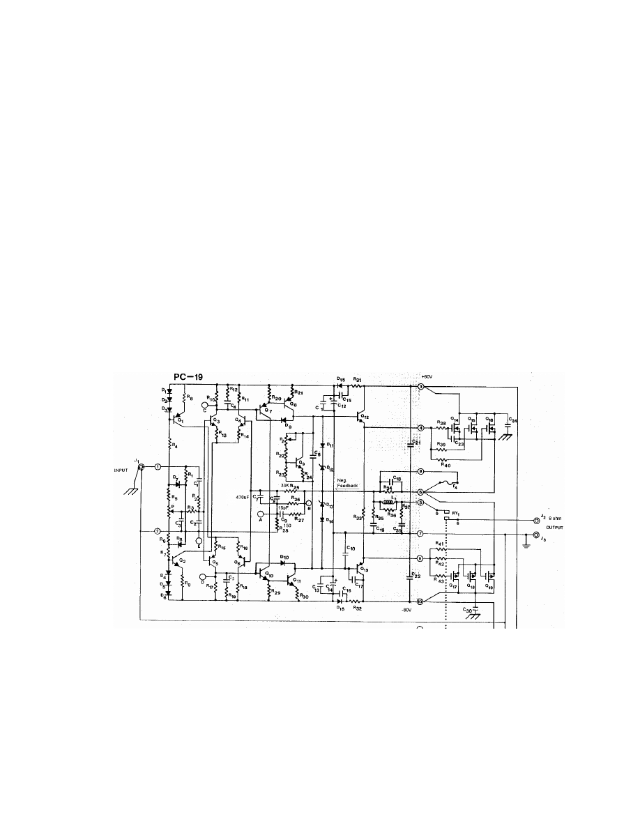
Fig. 1-9 Hafler DH500 audio power amplifier schematic, one channel shown.

22
components near the center of Fig 1-9 at a very low frequency ~0.01Hz
(
)
)
33
(
*
1
.
0
470
*
2
1
Ω
Π
=
K
uF
uF
f
c
. A differential stage sums in the feedback, followed
by a Darlington voltage amplifier. The output transistors are biased on to ~1 W by
biasing the output driver transistor into partial conduction to help prevent crossover
distortion due to the low Gm of the MOSFETs near cut-off. Symmetry between the N
and P channel MOSFETs is limited and negative feedback is required to reduce the large
3
rd
harmonic distortion that would otherwise be present. Transconductance drift with
temperature is not shown on the data sheets. Two points were tested, ambient and 100C°.
Results show reasonable tracking, promising that output stage shifts during transient
thermal effects do not tax the feedback loop excessively as this type of non-linearity is
truly non-harmonic.
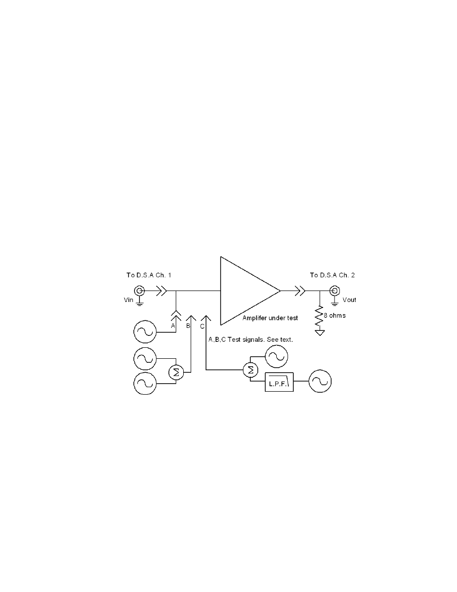
Measurements where performed by instrumenting the Hafler DH500 in the
following manner, shown in Fig. 1-10. Measurements where taken with the $26,000
Hewlett-Packard 35670A Dynamic Signal Analyzer
13
. This instrument is this the state-of-
the-art in terms of un-averaged on-screen resolution, with its front end meeting
specification over 75dB dynamic range. Averaging the sweeps affords another 30-40dB
dynamic range. The instrument includes un-weighted standard T.H.D analysis of up to 20
harmonics, and a low distortion signal source of large signal swing and offset, and 4
13
Graciously lent to my home lab by my employer, M.I.T. The D.S.A. was originally purchased for R&D
in the S.S.C. laboratories.
23
floating input channels. The required test signals for the standard measurements are
generated by either the HP35670A internal sine source shown as connection A in Fig.
1-10, a Singer TTG-3 two tone generator shown as connection B, or a combination of one
tone of the TTG-3 and a HP 8116A 50MHz pulse generator shown as connection C. The
L.P.F. (low pass filter) is required for the D.I.M tests and is a 6dB/octave passive network
with a –3dB point of 20kHz. The D.S.A. is used in two channel mode, with the test signal
input on Ch. 1 and the amplifier under test output on Ch.2. The ability to measure the
distortion of the input test signal in real time allows any residual distortion of the test
Fig. 1-10. Block digram of test set-up.
signals to be nulled-out in post-processing. The amplifier is loaded by a standard 8ohm
resistive load. The Hafler DH500 measurements are shown following. Frequency
response was less than 1db down at 20kHz and is not shown. One kHz THD was less
24
X:1 kHz
Y:16.657 Vrms
B:CH2 Pwr Spec
20
Vrms
20
uVrms
LogMag
6
decades
0Hz
12.8kHz
AVG: 3
THD:0.0074 %
Fig 1-11 DH500 Distortion components and T.H.D at 1 kHz, 32W.
X:15.016 kHz
Y:13.7843 Vrms
B: CH2 Pwr Spec
9kHz
60.2kHz
AVG: 10
20
Vrms
20
uVrms
LogMag
6
decades
THD:0.0246 %
Fig. 1-12 DH500 Distortion components and T.H.D at 15 kHz, 23W.
than 0.01% at output powers to 200W. Shown in Fig 1-11 is 32W, 1kHz. At 15kHz &
23W the second harmonic is at 0.026%, shown in Fig. 1-12. The previous two
measurements used the HP35670A internal source, connection A on Fig. 1-10.
Intermodulation measurements gave excellent results. Connection B in Fig. 1-10 is used,
and the test generator tones are set per the requirements of the specific coomom I.M.
tests. I.M. 200:7K at 1:1 ratio showed no static intermodulation products. I.M. 4K:15K
25
again shows flawless I.M. performance, shown in Fig. 1-13. The upper trace is an FFT
of the input signal showing the self I.M.D. of the signal generator/mixer. The lower trace
2kHz
27.6kHz
AVG: 7
A: CH1 Pwr Spec
X:3.136 kHz
Y:290.258 mVrms
1
Vrms
1
uVrms
LogMag
6
decades
X:3.136 kHz
Y:5.72462 Vrms
B: CH2 Pwr Spec
10
Vrms
10
uVrms
LogMag
6
decades
2kHz
27.6kHz
AVG: 7
Fig 1-13. DH500 Intermodulation Distortion, 4kHz:15kHz at 4W.
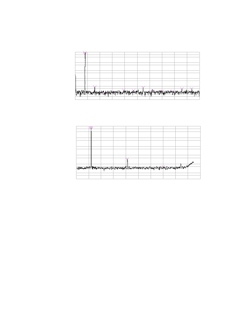
is the output of the DH500 at 4W. No additional IM products are discernable. Dynamic
intermodulation (D.I.M.) tests used connection C in Fig. 1-10. D.I.M. 3.18kHz:15kHz the
DH500 also did not add measurable dynamic IM products, as shown in Fig. 1-14. Again,
the upper trace is the input/test signal, the lower trace the amplifier output, with the
3.18kHz sine at 10W R.M.S. Comparing Figures 1-13 and 1-14 show that no additional
D.I.M. is measurable in the amplifiers output when the 15kHz square wave is modulated
26
2kHz
27.6kHz
AVG: 10
A: CH1 Pwr Spec
X:3.136 kHz
Y:456.988 mVrms
1
Vrms
1
uVrms
LogMag
6
decades
X:3.136 kHz
Y:9.0135 Vrms
B: CH2 Pwr Spec
10
Vrms
10
uVrms
LogMag
6
decades
2kHz
27.6kHz
AVG: 10
Fig. 1-14 DH500. D.I.M, per Otala, 3.18kHz:15kHz,10W
with the 3.18kHz sine, as per M. Otala’s procedure. This amplifier tests flawlessly in all
standard tests.
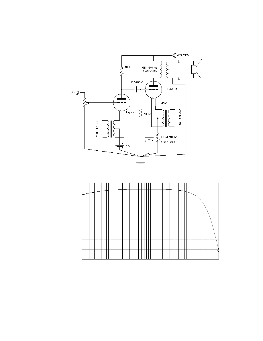
The second amplifier that is fully detailed is a 1.5W per channel single-
ended tube amplifier designed by myself using type 45 directly heated triodes developed
in 1926. The type 45 produces the most linear open loop transfer characteristic
14
over a
large portion of its operating range of any device I have tested, solid state or otherwise.
The type 45 was designed for audio frequency power amplification and can withstand
14
In Chapter 2 I show that the open-loop behavior of an amplifying element strongly determines the end
circuits subjective sound quality.

27
275V on its plate, can sink 36mA, and has a gain of 3.5 Siemens. The amplifier is
designed to present the output tube with its ideal load of 5800 ohms via the use of a very
high quality output transformer. A short discussion of the theoretical merits of the single
ended output stage is necessary. Accepting the use of an antique triode because of its
open loop linearity forces us to use an impedance matching transformer, which is
common. A transformer is nearly perfectly linear except for the region near zero flux and
near saturation. In both these regimes the slope of the BH curve is lower than in the linear
region. If the signal traverses the region near zero flux odd-order harmonic distortion is
produced. In Chapter 2 section 1 it is discussed that this distortion is audible and in
Chapter 2 section 5 it is explained in detail why the use of negative feedback is not a
solution to this non-linearity. A single ended design by its nature sinks a DC current of
half the peak current thru the output transformer. This forces the operating range away
from the two non-linear zones. The schematic is shown in Fig. 2-6. The driver stage is
necessary to match the voltage gain to the DH500 previously discussed. The type 26
directly heated triode was again chosen for its linearity. The gain of the driver is set to
times 35. Measurements where taken with the same setup as the Hafler DH550, shown in
Fig. 1-10. The load is the same 8 ohms. The finished amplifier has a respectable full
power frequency response of +/-0.5dB 20Hz to 15kHz shown in Fig. 1-15. This plot is
generated by a sweeping function of the HP 35670A. The –3db HF point is >30kHz.
28
Fig. 1-15. Schematic of the type 45 triode tube based Single-ended audio amplifier
20Hz
50kHz
-6.4
dBVrms
dB Mag
1
dB
/div
Fig. 1-16. Type 45 S.E. amplifier frequency response.
29
B: CH2 Pwr Spec
0Hz
12.8kHz
AVG: 4
10
Vrms
1
uVrms
LogMag
7
decades
THD:1.3578 %
Fig. 1-17. Type 45 S.E. amplifier 1kHz harmonic distortion components at 0.4W
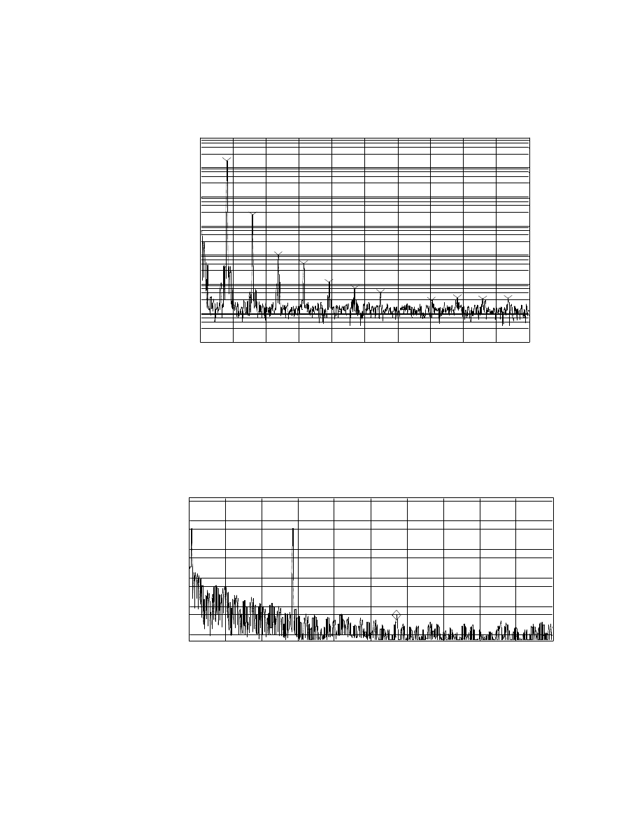
T.H.D. with a 1kHz sine input was 1.36% at 0.4W output, shown in Fig. 1-17.
Connection A on Fig. 1-10 is used. Note the 60Hz AC filament heater noise creates
closely spaced I.M. products around the harmonics. The 200Hz-7kHz I.M. performance
X:14.676 kHz
Y:44.8044 uVrms
B:CH2 Pwr Spec
600
mVrms
6
uVrms
LogMag
5
decades
100Hz
25.7kHz
AVG: 10
THD:0 %
Fig 1-18. Type 45 S.E. amplifier 200Hz-7kHz IM.
30
X:13.1 kHz
Y:264.872 uVrms
B:CH2 Pwr Spec
1
Vrms
1
uVrms
LogMag
6
decades
10kHz
16.4kHz
AVG: 10
Fig. 1-19. Type 45 S.E. amplifier 14kHz:15kHz IM.
was 0.08% as shown in Fig 1-17. IM using 14kHz:15kHz is shown in Fig. 1-19. The IM
product at 13kHz is 264 uV compared to the 14& 15 kHz at 637mV. This is less than
0.0001%. Static I.M. measurements used connection B on Fig 1-10. The D.I.M tests at
2kHz
27.6kHz
AVG: 10
A: CH1 Pwr Spec X:3.136 kHz
Y:391.98 mVrms
1
Vrms
1
uVrms
LogMag
6
decades
X:11.84 kHz
Y:8.33784 mVrms
B: CH2 Pwr Spec
10
Vrms
10
uVrms
LogMag
6
decades
2kHz
27.6kHz
AVG: 10
Fig. 1-20. Type 45 S.E. amplifier D.I.M.

31
higher power outputs show significant static IM products, as shown in Fig. 1-20. What
is notable is that when the 3.14kHz triangle wave was changed to a square wave no
additional IM products where detectable. This exact similarity between the static and
dynamic IM measurements is due to the lack of any negative feedback in this amplifier.
There is no mechanism to create intermodulation other than the first pass through the gain
devices non-linearity.
4. Conclusion. A call for a new methodology
The previous standard measurements clearly show the perfection of the high
power solid- state design and the horrible “performance” of the zero feedback. Yet, in
listening tests
15
, the single ended tube amplifier was unanimously judged as sounding
closer to the truth. It seemed more dynamic. It had less “grain”
16
, especially in the mid-
range. It seemingly had higher resolution as it presents a better “imaging”
17
sound field.
There has been a failure in the attempt to use specifications to characterize the
subtleties of sonic performance. Amplifiers with similar measurements are not
15
Although a strict scientific experiment was conducted comparing the amplifiers I do not present an
detailed analysis here. In summary, the type 45 amplifier was chosen as preferable 100% of the time by all
the different listeners (5) in a “single-blind environment”, meaning, the listener toggled a remote push
button and either the amplifiers were swapped or not. A numeric display was incremented at each selection
and the listener noted if the amplifier changed or not, and if the change was to the one preferred. I attended
all sessions and verified that levels where matched, that there was no clipping, and the program material
kept within the flat pass-band of the type 45 amplifier-speaker combination. The source was a live piano
microphone feed.
16
The audiophile press has varied colloquialisms to describe sound coloration. “Grain” is a common term
referring to a the interpretation of low level non-harmonic noise added to the signal.
17
“Imaging” refers to the clarity of the perceived stereo sound field. Commonly the better the “imaging”
the easier the listener can resolve the spatial locations of individual instruments.

32
equal, and products with higher power, wider bandwidth, and lower distortion do
not necessarily sound better. For a long time there has been faith in the technical
community that eventually some objective analysis would reconcile critical
listeners subjective experience with laboratory measurement. Maximum intrinsic
linearity is desired. This is the performance of the gain stages before feedback is
applied. Experience suggests that feedback is a subtractive process; it removes
distortion from the signal, but apparently some information as well. In many
older designs, poor intrinsic linearity has been corrected out by large application
of feedback, resulting in loss of warmth, space, and detail.
18, [25]
Over the past 10 years a clear trend has surfaced; designs at the higher end of cost in a
product line are enjoying decreased amounts of feedback, possible through the use of
more linear gain stages. In all recent cases, these quality products measure significantly
poorer in all accepted mainstream tests. Examples are the $15,000.00 Conrad-Johnson
companies model ART where the design chose 0 feedback over the design goal of
reducing the previous generations 12db of NFB to 3db. This minimalist single stage
design measures worse than their entry level products. The Cary Audio 805c has an
adjustable feedback selector – 6dB, 3dB, 1.5dB, and 0, with 0 setting receiving
widespread praise as “removing the pervasive graying of expression”
[26].
The Audio
Research Reference line is another example of a product that uses less gain stages at a
premium price. Even the marketing dictated major hi-end hi-fidelity equipment
manufacturing companies of Mark Levinson, Cello and Krell are moving toward more
linear gain blocks allowing for lowered feedback levels. All this movement is in strict
18
A quote by Nelson Pass, President of Pass Laboratories, from the Passlabs.com website. Mr. Pass is one
of the most prolific inventors in audio. He designed all the Threshold and Phase Linear line. Pass
Laboratories specializes in large MOSFET based single-ended audio amplifiers and pre-amplifiers.

33
opposition to the current, standard, accepted measurements that drive “specifications”.
This trend indicates that there needs to be a revision to the current measurement
methodology if the goal of audio equipment specification is correlation with subjective
sound quality.

34
CHAPTER II
A NEW AUDIO TEST PHILOSOPHY
Offered are my precepts that lead to a new test methodology that derives
results that better correlate with subjective sound quality. These are examined in the
subsections following.
1) The ears’ self generated harmonics mask external harmonic distortion that has the
same character. The ears’ harmonic distortion is fully studied and falls off at a rate of
approximately 10
n
, where the power
n
designates the harmonic number. I propose
that external harmonics strictly adhering to this envelope are fully “undistorted” by
our ear-brain system and are thus indistinguishable from pure tones. An analytical
derivation of conformance to this aural harmonic envelope is developed.
2) The increase of aural harmonics follow sound pressure level increases non-linearly
and at different rates per harmonic. Therefore absolute system S.P.L.
19
must be
considered.
3) Intermodulation distortion is masked by this same mechanism. Amplifier topologies
exist that are free from dynamic intermodulation affects, and whose residual
intermodulation is linearly related to harmonic distortions.
19
Sound Pressure Level.

35
4) The character of the noise envelope within a sound transient is important to the
brains recognition system. Noise floor pollution via low level high order I.M.
products are to be avoided.
5) No current standard static or dynamic tests or other instrumentation based
measurements correlate sound quality with levels of negative feedback. There is
ample correlation between harmonic measurements and sound quality with devices
that use no negative feedback (transducers and zero feedback electronics). It is
proposed that audio gain stages be analyzed using weighted
20
T.H.D, I.M.D., and
other tests, with all loop feedback disconnected.
1.
Harmonic Consonance.
The cochlea is the potion of the inner ear devoted to hearing. It is a 35 mm long spiral
fluid filled tunnel of reducing aperture embedded in bone with 12,000 outer hair cells
spread every 10 microns in sets of 4, each tuned to a different frequency. Studies via
instrumenting
21
sets of outer hair cell neurons have verified the creation of harmonics
within the cochlea, documented in the 1924 figure
[28]
Fig. 2-1. This work is the result of
20
As notes in previous sections, higher order harmonics are increasingly more detectable by the ear-brain
system as audible distortion.
21
Studies where performed on cats
[27]
. No studies where found on the human ear system that directly
measured the hair cell transducer harmonics due to the mechanical limitations of the hair-cochlea interface.
The geometry and cell type are very similar, and, other indirect methods of measuring the aural harmoincs
have been thoroughly developed.
36
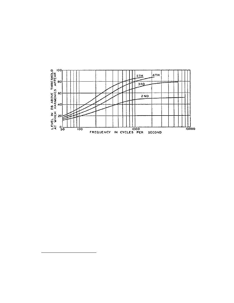
speech recognition studies. Shown are the ears self created harmonics relative intensity
versus fundamental frequency. The data was derived by using the understood
Fig 2-1. Ear self-generated harmonics, frequency versus level.
phenomenon of hearing beating when two notes are impressed on the ear. An auxiliary
tone of a frequency near the fundamental test tones’ harmonic is used and its level raised
until beating is just audible. This level is related to the ears natural aural harmonic
creation. Inspecting this data, the second harmonic of a 1kHz fundamental tone
22
is 50dB
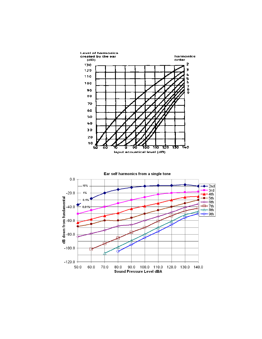
above the threshold of hearing. In 1967 Olson
[28]
from RCA/Victor R&D Labs continued
testing the first 8 harmonics and over a broad range of sound pressure levels, reproduced
here in Fig. 2-2. This has been redrawn for clarity in Fig 2-3. Notice that the ear creates
significant levels of the second harmonic, nearly 10% of the fundamental for sound
pressure levels (SPL’s) of 90dBA and above. Also the slope of the harmonic
22
The sound pressure level was not cited in this work. One assumes speech level, ~70dBA.
37
Fig. 2-2. Ear self-generated harmonics, level versus sound pressure level
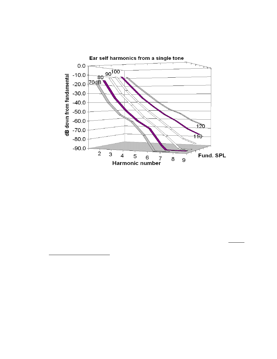
Fig. 2-3. Ear self-generated harmonics, level versus sound pressure level
38
Fig.2-4. Subset of Fig. 2-3 with reduced SPL range for clarity
reduction versus input reduction varies with the harmonic power, beginning at
approximately 1:10 for the 3
rd
harmonic to 1:1 for the 9
th
harmonic. A different
perspective is shown in Fig 2-4. A reduced SPL range is shown. Even for the moderate
S.P.L. of 80dBA, the 2
nd
harmonic is at the equivalent of 65dBA or normal voice level,
and the 3
rd
at 45dB. This is still ~40dB above the mid-band threshold of hearing, yet one
does not hear the harmonics! Only a single pure tone is heard. The ear/brain appears to be
able to completely suppress the sound of a range of harmonics if they conform to this
specific pattern. This pattern is the aural harmonic envelope. It follows that this same
mechanism will mask harmonics arising in the sound reproduction chain if they follow
this pattern. If the harmonics do not follow this pattern, the ear brain indeed detects these
39
as new tones. Therefore, for all but extreme frequencies and sound pressure levels, any
electronics that generate this harmonically consonant envelope will be transparent.
Previous work has shown that people had a strong preference for a signal with 0.3%
artificially injected even-harmonics that had 0.03% odd-ordered harmonics
[29]
. Note that
for the predominant 2
nd
and 3
rd
harmonic this better mimics the aural harmonics.
The above discussions are conscious of the well understood ear’s
phenomenon of masking, where low level tones in close proximity to a higher level tone
remain unheard. This masking effect was thought by some
23
to be one of the rationales
for weighting the higher order harmonics stronger in weighted T.H.D. measurements.
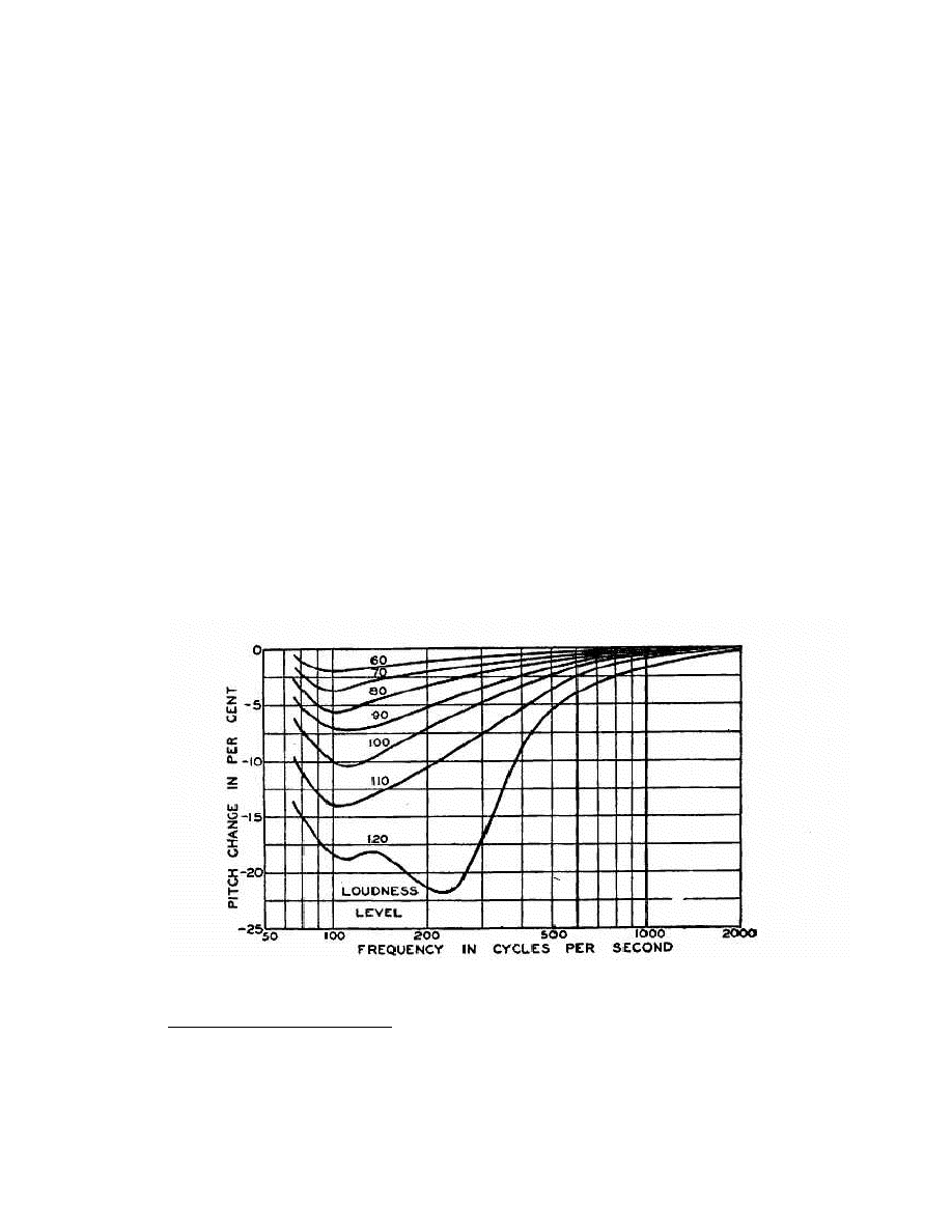
Fig. 2-5
[33]
following
shows the pitch change necessary to distinguish a second tone. Note
Fig. 2-5 Pitch change necessary to distinguish a second tone
23
References [30], [31], [32]
40
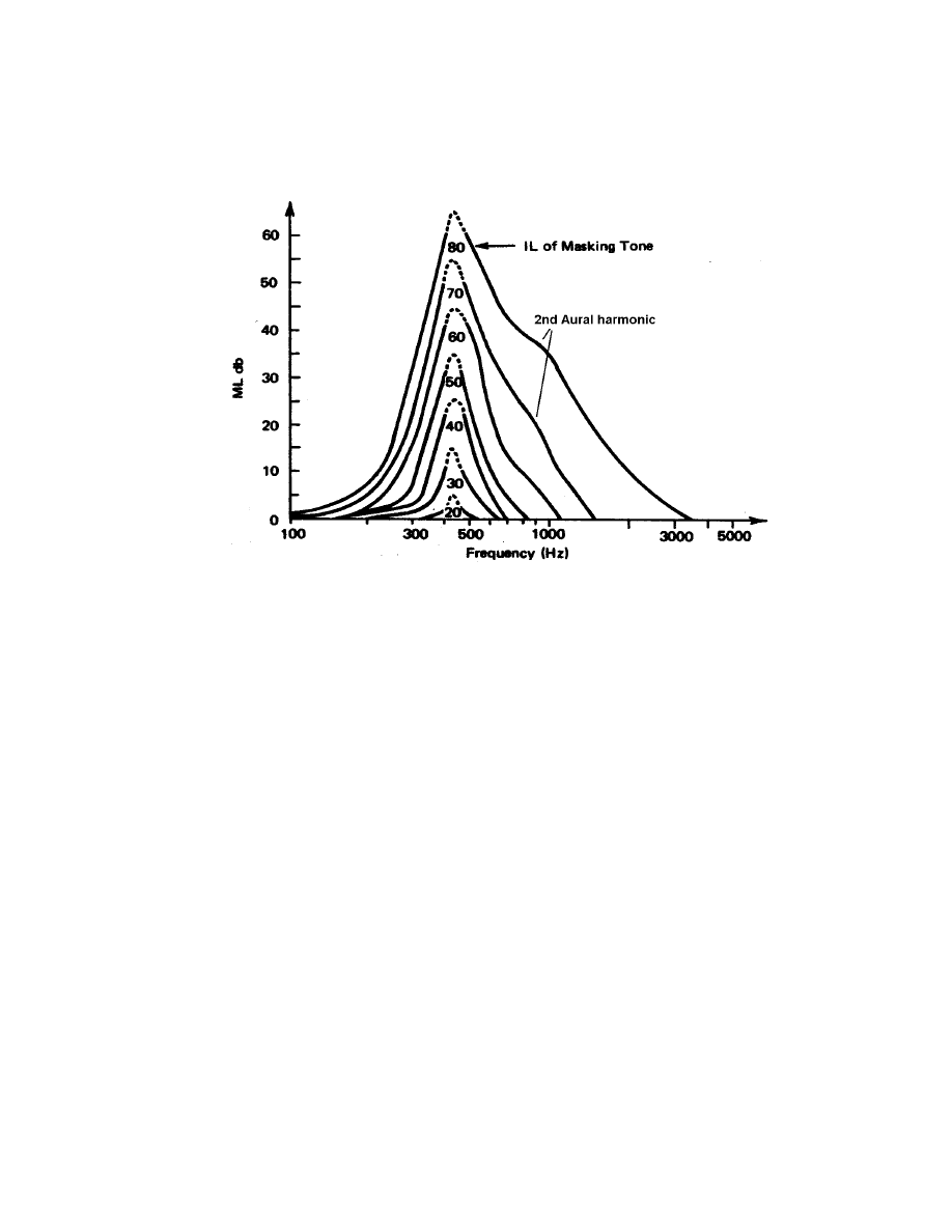
Fig. 2-6. Tone masking research showing aural harmonics
that harmonics are at 100% pitch change. Fig. 2-6
[34]
actually shows that the aural
harmonics have a stronger influence than masking, note the lack of symmetry about the
fundamental (415Hz) and the shoulders of the 2
nd
harmonic. The aural harmonics play a
more prominent role than the ears masking mechanism. There was no correlation
between age and sex in these or other studies of aural harmonics. There are significant
sex and age differences on most other aspects of hearing, namely frequency extension.
These are due to the macro effects such as ear tunnel geometry or exposure damage.
These effects are not investigated herein as they are presumably not involved with the
ear-brains system of self-correcting for the aural harmonics.

41
2. The sound pressure level dependence of the aural harmonic envelope.
The dynamic range of individual hair cell neural output is about 10
3
, while
the range of audible sound pressure levels is about 10
5
. The latest studies have shown that
the hair cells’ length is modulated by the neural voltage and this is believed to explain the
compression
[36]
. As was shown is the preceding section the aural harmonics do not fall
off at the same slope either by harmonic number or linearly with decreasing sound
pressure levels. For rising S.P.L.’s the ear creates a monotonically reduced steepness
pattern. We cannot disregard this function of the ear. For example, if the ear is presented
with an auxiliary sound distorted with a set of harmonics that are consonant with the
aural harmonics at 100 dBA
24
but the actual sound pressure level of the fundamental is
say 10 or 100 times (10 or 20dB) less, it will be perceived as distorted. The Eq. 2-1 which
11
)
22
(
10
*
35
.
1
%
n
n
F
dBA
=
Eq. 2-1
Where: %F
n
= Aural Harmonic Amplitude in % of Fundamental for the n
th
harmonic.
dBA = Decibels “A” weighted Sound Pressure Level resultant from the
Fundamental.
n = The harmonic number. f = nF
f
where f is frequency,
F
f
= fundamental frequency
24
dBA is the commonly used absolute measure of loudness for humans. It is filtered by an approximate
inverse of the ears sensitivity variations over frequnency. The A designates the standardized A weight
filter.
42
I derived myself
25
from the Olson data is presented and takes the sound pressure level
variation into account. It is a mathematical expression relating the percentage of the
fundamental S.P.L. of the ears self distortion, per harmonic, relative to the sound field
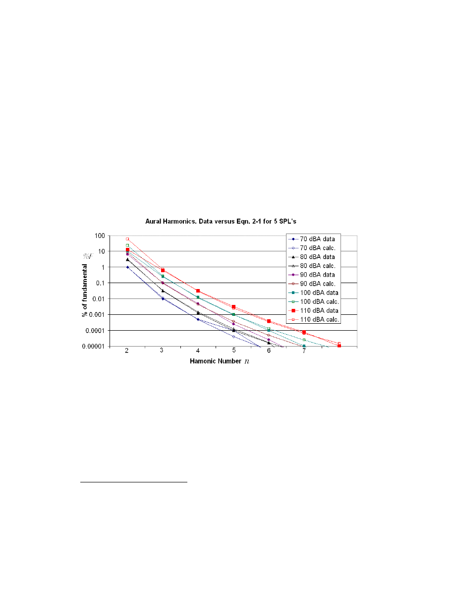
S.P.L. The power of the exponentiation may seem high but the fit is excellent, shown
following in Fig. 2-7. The solid data points are the data taken directly from the Olson
figure reproduced earlier as Fig. 2-2. The hollow data points are calculated from Eq. 2-1.
Fig. 2-7 Showing fit of Eq. 2-1 versus Olson aural harmonic test data
[28]
.
For the highest SPL's a compression of the 2
nd
aural harmonic is noticed. This error of the
fit is acceptable as these levels are very high. For normal music reproduction in the home
(levels of 90dBA peak) the fit is very good, to 0.0001% of fundamental, or about 30dBA,
which is below the noise floor of a normal listening environment. An ideal amplifier
25
This equation was derived by first using curve fitting algorithms and then hand manipulated using
spread-sheet tools until the error bars where minimized.

43
would contain no harmonics that do not conform to this aural harmonic envelope. It is
proposed that the relative deviation between an amplifiers distortion harmonics and the
aural harmonics, per harmonic, must better quantify the detectable error of the amplifier
and therefore the subjective sound quality of an amplifier. The better sounding amplifier
will have either no harmonics or those that are present must strictly conform to the aural
harmonic envelope. In testing many different amplifiers their harmonic signature did not
follow the aural harmonic envelope. Universally the distortion has high order harmonics
without the next lower order harmonics’ complementary level. Contrary to the history
and evolution in audio design, high order harmonics, if they appear, MUST be joined by
a family of lower order harmonics that follow the aural harmonic envelope. In calculating
the magnitude of an amplifiers deviation for the aural harmonic envelope I propose that
each harmonics deviation be on a relative basis (% of reading, referenced to the level of
the n
th
aural harmonic derived from Eq. 2-1), rather than on the absolute percentage
referenced to the fundamentals level. This puts a very strong weighting on the higher
harmonics and thus demands state-of-the art signal to noise ratios in the instrumentation.
The $29,000 H/P 3458 Dynamic Signal Analyzer used for this thesis is state of the art,
with a 5 decade on-screen dynamic range. This limitation corresponds to approximately
0.001% of fundamental
26
. This limitation is reasonable, in that the S.P.L of the amplifiers
26
The dynamic range of a spectrum analyzer can be extended by the use of a calibrated notch or steep high-
pass filter to remove the fundamental. This technique was not used herein mainly due to the wish to
correlate all the readings for all the amplifiers tested at all frequencies without individual normalization.

44
harmonics at the 0.001% level are very near the threshold of hearing for moderate
listening levels. The equation below has been developed for calculating a so named Total
Aural Disconsonance, or T.A.D, a dimensionless figure of merit.
∑
=
−
=
20
2
2
11
22
10
*
35
.
1
1
.
.
n
dBA
n
n
H
D
A
T
Eq. 2-2.
Where: T.A.D. = Total Aural Disconsonance, the r.m.s. sum of the absolute
deviation of an amplifiers n harmonics from the aural harmonics.
n = Harmonic number. Usually does not exceed 20.
H
n
= measured level, in % of Fundamental, of the n
th
amplifier harmonic
NOTE: if the denominator,
11
22
10
*
35
.
1
n
dBA
, is less than the noise floor, then it
should be replaced with the noise floor.
The T.A.D. figure can be quoted alone, the goal of a generalized method of documenting
audio amplifier quality. Many previous attempts at better correlating subjective quality
with measurements, as previously discussed, have recommended either the weighting of
harmonics components in the T.H.D calculation or specifying individual harmonics’ %
distortion. The T.A.D. method is the first to use psycho-acoustic based data to weight the
individual harmonics. The range of amplifier T.A.D figures can be 100 for very good to
10,000 for very flawed. Several proposed methods of calculating T.A.D. follow.

45
1. By inspection.
A spectrum analyzer of sufficient dynamic range performs the measurements. The
individual harmonic levels, in % of fundamental, are divided by the data in Figs 2-2 or 2-
3 or Table A-1 in the Appendix. This results in a percent deviation per harmonic relative
to the aural harmonic level. An R.M.S. sum is performed to result in the dimensionless
T.A.D. For example lets examine the conformity to the aural harmonics of the two
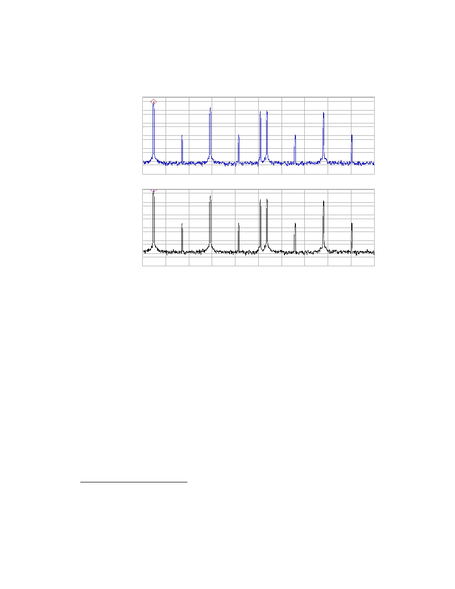
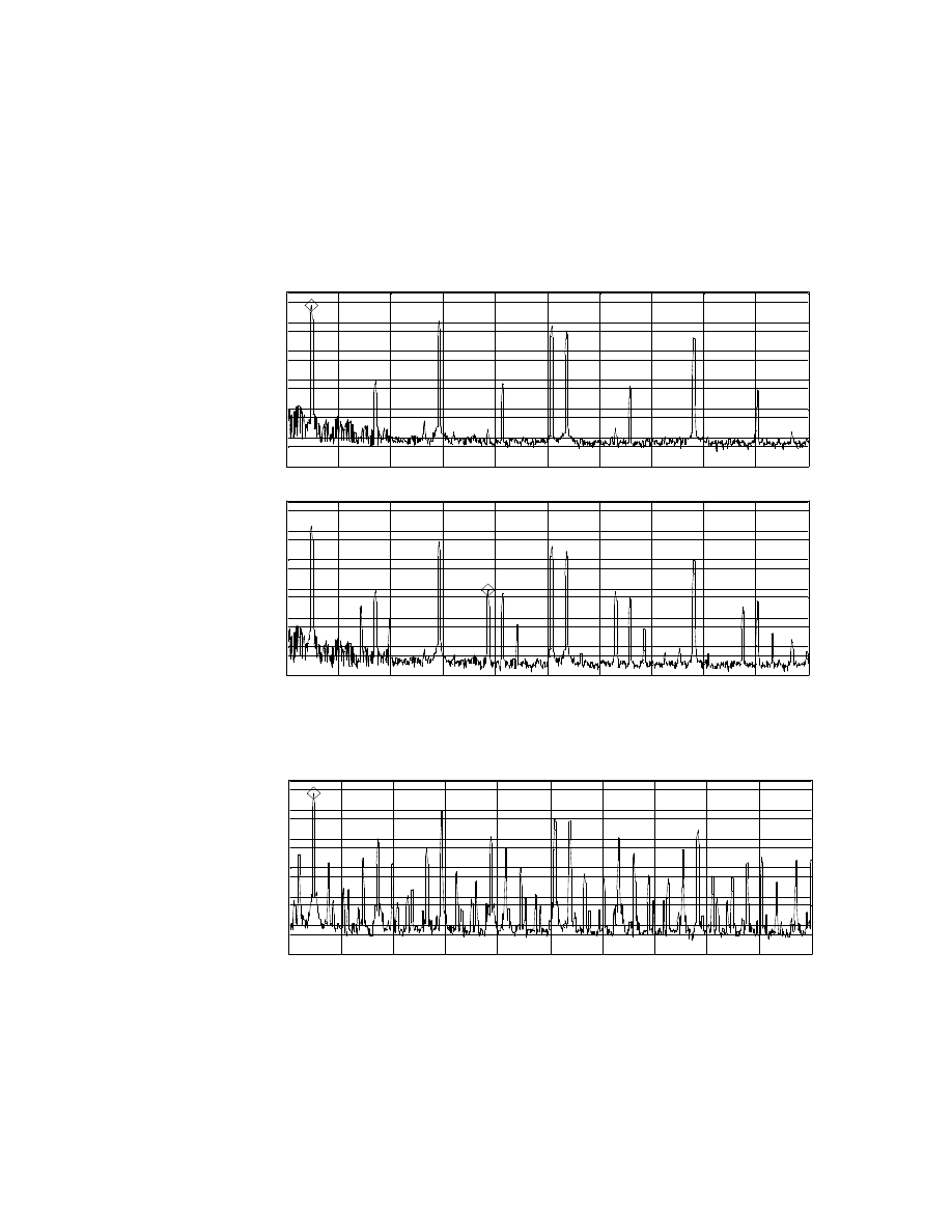
amplifiers harmonic distortion shown below. The first is the single-ended type 45 Triode
amplifier from Chapter 1, followed by a 10W bi-polar push-pull feedback amplifier of
marginal quality. Output powers at the measurements taken where 0.32W and 0.72W
respectively (the distribution of the harmonics of either amplifier remained similar at
matched output). Using a moderate to high efficiency speaker of 95dBA/1W/1m at near-
field the respective fundamental S.P.L is 91dBA and 94dBA respectively. Using equation
Eq. 2-1 the following aural harmonics are created at these S.P.L’s. The amplifier
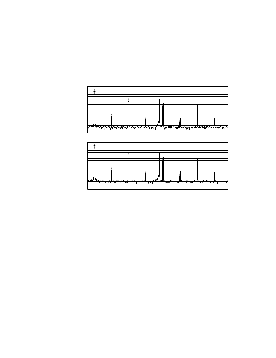
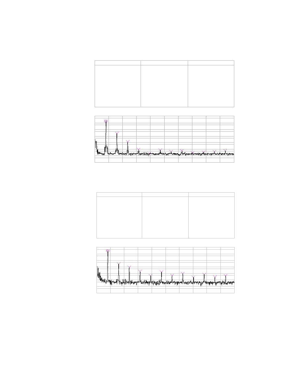
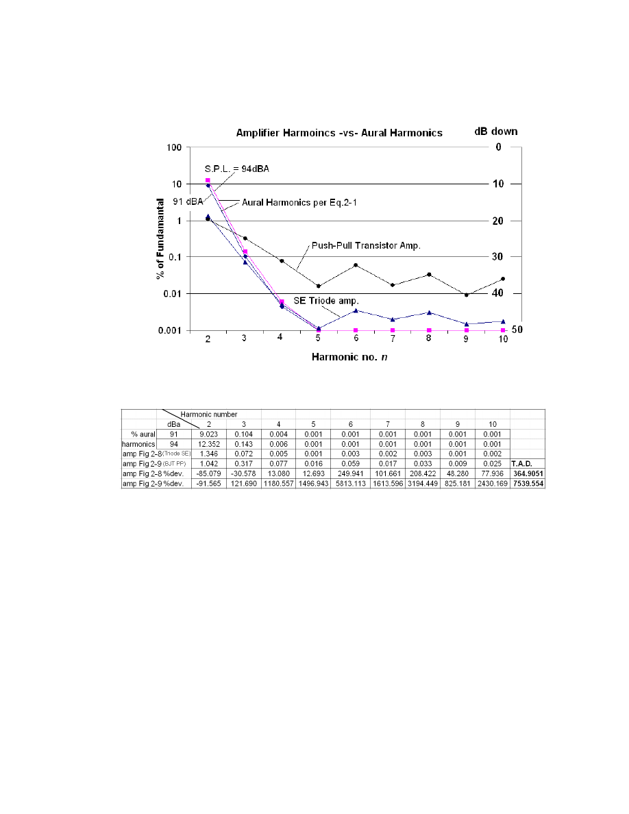
measurements shown in Figures 2-8 & 2-9, summarized in Fig. 2-10, and the resulting
Total Aural Disconsonance is derived and tabulated in Table 2-1. The resulting T.A.D is
365 for the triode amplifier and 7540 for the transistor amp. Indeed the Single ended
triode power amplifier, with the lower T.A.D. figure sounded far superior to the low
quality transistor amplifier with the most significant improvement being freedom from
46
Entry Label
Hz
Vrms
Fundamental
1
k
1.686
2nd
2
k
22.742
m
3rd
3
k
1.221
m
4th
4
k
84.476
u
5th
5
k
19.106
u
6th
6
k
59.731
u
7th
7
k
34.871
u
8th
8
k
52.586
u
9th
9
k
25.253
u
10th
10
k
30.643
u
AVG: 10
A: CH2 Pwr Spec
X:1 kHz
Y:1.68553 Vrms
LogMag
X:1 kHz
Y:1.68553 Vrms
B: CH2 Pwr Spec
10
Vrms
1
uVrms
LogMag
7
decades
0Hz
12.8kHz
AVG: 10
THD:1.3512 %
Fig. 2-8 1.5W Type 45 Triode feedback-less single-ended amplifier at 0.32 W rms.
Entry Label
Hz
Vrms
Fundamental
1
k
2.486
2nd
2
k
25.926
m
3rd
3
k
7.872
m
4th
4
k
1.972
m
5th
5
k
397.03
u
6th
6
k
1.467
m
7th
7
k
426.504
u
8th
8
k
819.455
u
9th
9
k
230.985
u
10th
10
k
629.134
u
AVG: 3
A: CH2 Pwr Spec
X:1 kHz
Y:2.48566 Vrms
LogMag
X:1 kHz
Y:2.48566 Vrms
B: CH2 Pwr Spec
10
Vrms
1
uVrms
LogMag
7
decades
0Hz
12.8kHz
AVG: 3
THD:1.0958 %
Fig. 2-9 10W Bi-polar transistor feedback amplifier at 0.72 W rms.
47
Fig 2-10. Two amplifiers distortion harmonics versus aural harmonics
Table 2-1. Spreadsheet based T.A.D calculations for two amplifiers.
any grainy “electronic” sounds. The triode amps reproduction seemed to come from an
absolutely quiet background and dynamics seemed improved, irregardless for the higher
static signal to noise level and lower output power. The amplifiers superiority was well
audible with most music. Most remarkable was the perceived instrument placement using

48
an all analog signal chain
27
. Note that the standard T.H.D. measurement, performed by
the D.S.A. to the 20
th
harmonic was 1.35% for the triode amplifier and 1.09% for the
transistor amplifier. The T.A.D. figure is much worse for the transistor amplifier, a result
of its high levels of high-order harmonic distortion.
2. Automated calculation of T.A.D.
Alternatively Eq. 2-1 calculates the individual harmonic levels in an automated T.A.D.
test system, built on a PC computer using a high-quality sound card and an automated test
software package like LabView. Ideally executed, a microphone could pick up the
systems’ loudspeaker output for direct reading of the fundamentals S.P.L. The entire
music reproduction system could be rated in terms of T.A.D. In this case, the amplifiers
distortion onset could be “tweaked” to minimize T.A.D. by changing loudspeaker
efficiency or loudspeaker proximity. A very low value of T.A.D would guarantee that the
reproduction systems sense of scale is realistic
28
.
27
Although outside of the scope of this research, the T.A.D. figure could include all elements of the signal
reproduction chain, including the storage technology. Perhaps the decimation required by digital recording
and playback alter the harmonic envelope. There is a controversial phenomenon where a LP record based
playback system seems to have greater resolution that the digital system in the face of 100 fold higher
signal to noise ratio. The most reasonable explanation may be that the current digital medium has higher
levels of signal correlated noise.
28
The change in slope of the aural harmonic envelope with intensity changes is well matched by feed-back
free triode amplifiers, who, are universally low powered. This “scale matching” may explain the non-
intuitive effect of increased dynamics with these type of amplifiers over amplifiers of much higher power
ratings.

49
3 . Intermodulation distortion
Universally accepted work has shown a fixed correlation between an audio
amplifiers static Intermodulation Distortion and its Harmonic Distortion characteristic
[14][15]
, including full mathematical derivations
[15]
. Alternatively, the ear generates
intermodulation products due to the same non-linearity that causes Aural Harmonics to
appear
[36]
. Therefore the same T.A.D. figure of merit quantifies the audio reproductions
devices’ audible IM distortion. T.I.M. or D.I.M (Transient I.M. or Dynamic I.M.) per M.
Otalas' extensive literature
[20][21][22]
has been shown to arise solely in feedback amplifiers
due to input or intermediate stage slew-rate induced phase errors. In my extensive tests of
zero feedback power amplifiers with even cascaded gain stages I was unable to measure
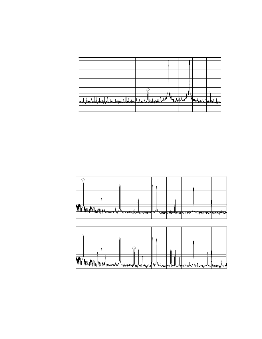
increased I.M. due to dynamic affects using the described methodology. Indeed the 10W
transistor amplifier showed the presence of D.I.M. Note the absence of intermediate I.M.
lines in the zero-feedback amplifier. Dynamic Signal Analyzer output is presented in the
following Fig’s 2-11 & 2-12. The upper trace in Fig. 2-11 are the test harmonics per M.
Otalas' “A Method for Measuring T.I.M.”, a 3.14KHz Square wave lowpass filtered at
30kHz summed with a 15kHz sine of ¼ the square waves level. The lower trace of Fig 2-
11 is the output of the type 45 triode amp, and Fig 2-12 the 10W transistor amp.
Importantly, the multiplicative nature of feedback in creating many IM products actually
50
raises the noise floor by almost a factor of 10 when the test signal is injected. With no
input the noise floor of the transistor amp was below the triode amp. These minor
2kHz
27.6kHz
AVG: 10
A: CH1 Pwr Spec
X:3.136 kHz
Y:391.98 mVrms
1
Vrms
1
uVrms
LogMag
6
decades
X:11.84 kHz
Y:8.33784 mVrms
B: CH2 Pwr Spec
10
Vrms
10
uVrms
LogMag
6
decades
2kHz
27.6kHz
AVG: 10
Fig. 2-11. D.I.M. measurement example for a non-feedback amplifier
X:3.152 kHz
Y:3.67492 Vrms
B: CH2 Pwr Spec
10
Vrms
10
uVrms
LogMag
6
decades
2kHz
27.6kHz
AVG: 10
Fig. 2-12. D.I.M. measurement example for a feedback amplifier

51
sub-harmonics modulate in their relative relation to each other with signal level and
could very well be responsible for the “grainy” sound associated with some high
feedback audio amplifiers. The D.I.M. method picks out the specific harmonics peak
amplitudes to calculate D.I.M. but does not specifically measure the noise floor for
further IM harmonics and sub-harmonics.
4. Pre-transient Noise Bursts.
The noise burst detected during the first few 10ths of a second in a complex
percussive sound like a piano or harpsichord has been shown to be a key element in the
recognition process
[37 pp. 153]
. The brain has a very complex multi-tone intelligibility
engine, but at a certain threshold the additional random vibrations (noise) the neural
processing mechanism simply gives up. I propose that feedback in and of itself creates
levels of intermodulation distortion that modulate and otherwise confuse the noise bursts
of musical instruments, leading to a subjective response that the sound is “artificial”. An
example would be the inability of even the finest instrumentation being able to quantify
the difference between a Stradivarius violin and a more modest instrument
[37 pp. 111]
.
Indeed the string player has the ability to introduce extremely fine changes in timbre. Our
brain has learned to build up the corresponding identifying readout patterns based on
tremendously refined information processing. We are able to recognize minute,
unmeasurable, fine structures of the acoustical signal. If these fine structures are
unmeasurable in the live acoustical field via a direct feed into the analyzing instrument it
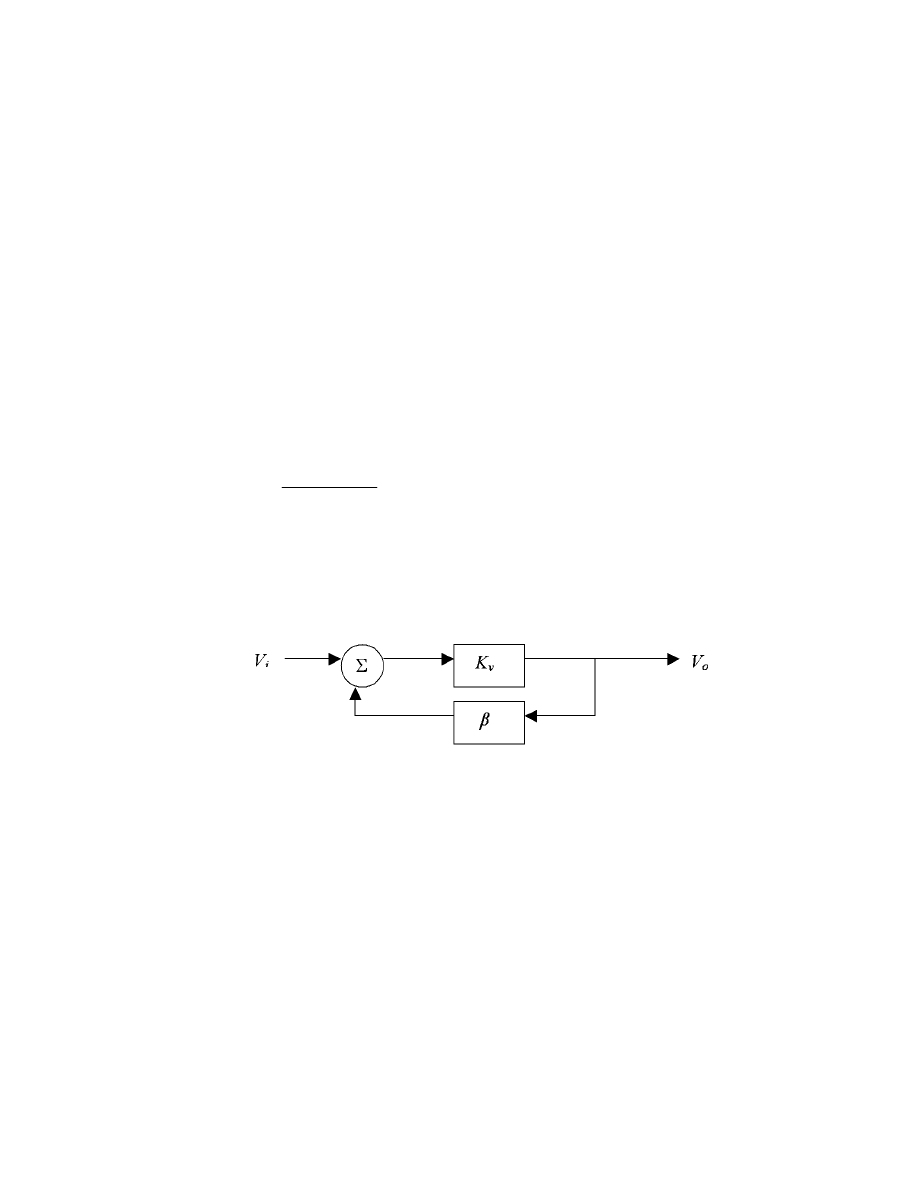
52
follows that we are unable to determine if electronics are transparent in this regard!
Indeed there exists currently no methodology that specifically analyzes the fidelity of a
noise burst buried in a tone transient.
5. The fallacy of negative feedback as a cure-all.
This section details the common but incorrect assumption that negative
feedback reduces non-linearity distortion in the same ratio as it reduces gain. This
assumption is true only if there is no non-linearity to reduce. To avoid confusion with
other work on feedback analysis I assign the following most common terms, K
v
is the
open loop transfer function of the gain block under analysis, and ß is the transfer function
of the feedback network, shown in the feedback block diagram Fig 2-13. In most modern
Fig. 2-13. Negative feedback block diagram
texts, these transfer functions are usually functions of frequency only. For example nearly
all op-amp analysis concentrates on stability margin using root-locus methods to predict
stability. Here we are concerned with the forward gain elements K
v
non-linearity and
assume that stability is present and operation is well within the pass-band. Indeed,

53
surprisingly, even phase shift is not involved in the analysis. Fig.2-13 is reduced to the
familiar closed loop transfer functions in Eq. 2-3.
β
β
−
=
−
=
v
v
v
i
o
K
K
K
V
V
1
1
1
Eq. 2-3.
This result allows us to further define the following important terms used in analyzing
and describing negative feedback systems.
Forward Loop Gain
= K
v
Loop gain
= ßK
v
= A
l
dB of feedback
= -20log|(1- A
l
)|
Two results of the application of negative feedback not related to the forward loop
linearity are bandwidth extension and output resistance reduction (Eq. 2-4). Their
derivation is straight forward and included in standard analog electronic circuits text
[38]
.
l
o
c
A
Z
Z
−
=
1
Eq. 2-4.
Where, Z
c
= closed loop output resistance, Z
o
= open
loop output resistance, A
l
= loop gain.
In the case of bandwidth extension, commonly this applies to gain stages that are rolled
off early by design to guarantee stability over a wide family of closed loop gains. In these
cases negative feedback is necessary to achieve adequate frequency response. Op-amps,

54
power op-amps and single chip audio power amplifiers fall under this classification
29
.
Their output stages are universally push-pull in strict class B as they do not use
complementary output devices and thus preclude some class AB bias scheme
[38]
. Open
loop these devices commonly are unstable due to their very high gain, and are far from
hi-fidelity.
A mathematical proof follows that convincingly illustrates that even
minimal amounts of negative feedback covert moderate amounts of low-order harmonic
and intermodulation distortion into a multitude of high-order distortion products. I
consider two classes of non-linearity, first, a parabolic transfer function that is closest to
the F.E.T and AF transmitter vacuum tubes, and secondly an exponential transfer
function that is very close to the ordinary junction transistor.
Consider an output gain device that departs from linearity only because of
the presence of a square law term in the transfer function, as shown below in Fig. 2-14.
Note how well this transfer characteristic follows a real device, a large N channel
MOSFET
30
. The X axis in Fig.2-14 is the voltage on the FET gate, V
gs
. This region
represents approximately 10% of the full current capability of the device, about 2 A.C.
watts. Also, for convenience the output is offset to start at zero, although significant
current is flowing throughout the shown range. With no feedback the transfer function
29
The National Semiconductor LM3886 for example. A 60W rms monolithic chip that retails for under $3.
The open loop frequency response is shown falling off before 100Hz
[39]
30
55Amp I
d
, 200V
brdss
. Motorola MTY55N20
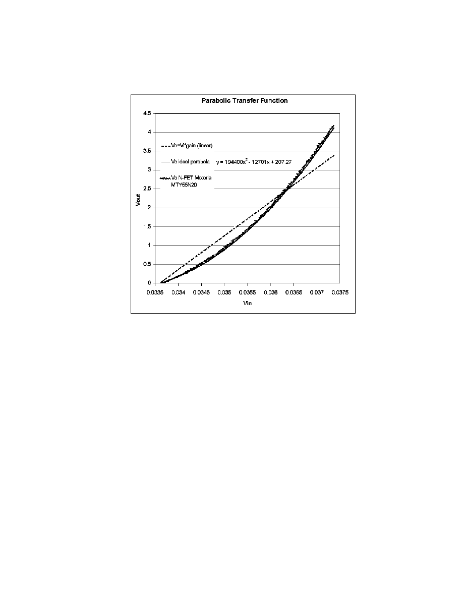
55
Fig. 2-14. Transconductance graph for a power field effect transistor.
can be written as:
(
)
2
in
in
out
Av
Av
v
α
+
=
Eq. 2-5
Adding feedback to a system necessitates separating the input from the portion after the
summing node, the portion that includes the negative feedback.
in
out
s
v
v
v
+
=
β
Eq. 2-6
Clearly if ß is increased the resultant transfer characteristic becomes more linear and at
limit the gain is given by:

56
β
1
−
=
in
out
v
v
Eq. 2-7
Adding feedback to a non-linear gain element creates modulation at the sum and
difference frequencies. In the case of the purely square term function, a single sine input
of frequency f creates only second harmonic distortion. As soon as some feedback is
applied a third harmonic appears, which is again fed back and creates sum products at
f+3f , or fourth harmonic, and 2f+3f , fifth harmonic. This previous discussion is intuitive
but can also be shown mathematically. To arrive at this one uses a power series to define
the closed loop (feedback included) transfer characteristic of the type:
...
4
4
3
3
2
2
1
+
+
+
+
=
in
in
in
in
out
v
a
v
a
v
a
v
a
v
Eq. 2-8.
To obtain the corresponding closed loop power series the feedback equation Eq. 2-6 is
substituted into the square term transfer characteristic Eq. 2-5. This produces a quadratic
equation relating v
in
and v
out
. To transform this into a power series the binomial theorem
is used. The resultant harmonic weights as a function of v
out
are shown in Table 2-2.
Harmonic
Number
Percentage of
fundamental
2
β
α
A
V
out
−
1
50
3
(
)
2
2
2
1
50
β
α
β
A
V
A
out
−
4
(
)
3
3
3
2
2
1
5
.
62
β
α
β
A
V
A
out
−

57
5
(
)
4
4
4
3
3
1
87.5
β
α
β
A
V
A
out
−
6
(
)
5
5
5
4
4
1
25
.
131
β
α
β
A
V
A
out
−
Table 2-2. Distortion components versus feedback level for a square law dominated gain
device
Note the strong function of output level V
out
of the higher harmonics. What is more subtly
hidden is the sharp increase of higher harmonics as even moderate feedback is applied.
Figure 2-13 following reveals this behavior over a broad range of feedback. Fig. 2-15 is
realized by fixing V
out
to ~2 Watts AC and plotting Table 2-1’s percentage of
fundamental per harmonic number versus the feedback factor, ß. a in the Fig. 2-15 is
designated in the somewhat more common k. In Chapter 3 actual device measurements
results of F.E.T’s and B.J.T.’s are included and show good agreement with the
calculations in this section although slight de-generation of the FET gate drive results in
some H3 and higher distortion with no feedback in place. The levels where at least a
factor of 10 below the sum-difference based feedback modulation “maximas” shown.
This data, when plotted along with the corresponding T.A.D. “Total Aural
Disconsonance” figure of merit, conclusions about proper level of negative feedback are
readily drawn.
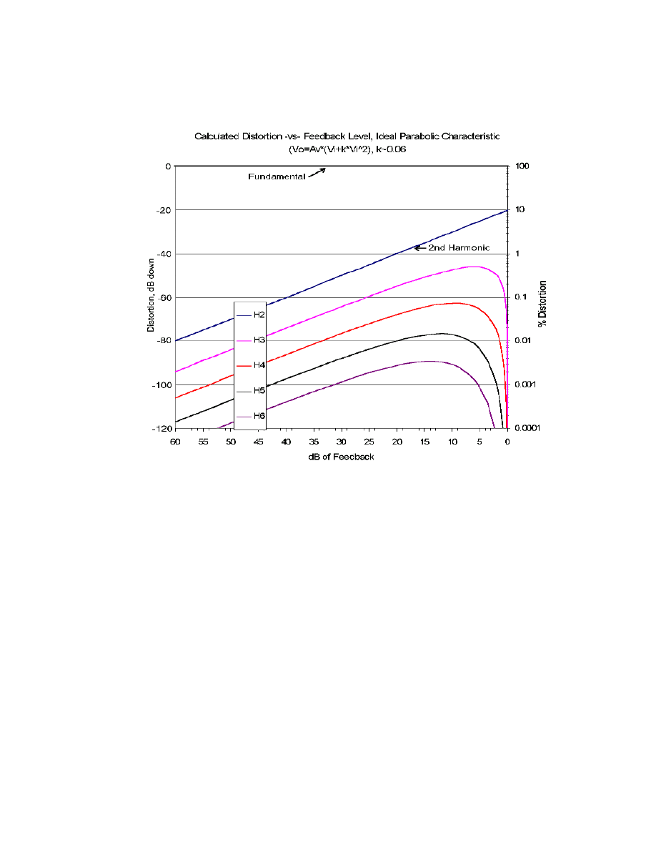
58
Fig 2-15. Calculated Distortion versus feedback level using the equations in Table 2-2.
In Fig 2-15 above note the sharp rise in the levels of distortion as only 3dB of negative
feedback is applied! More importantly note the minor reduction in the aurally benign 2
nd
harmonic versus the rise of the more disconsonant harmonics. For the plotted curves in
Fig. 2-15 a = .06, and the resulting zero-feedback 2
nd
harmonic distortion is 10%. This is
higher than the ears aural harmonics, and thus higher than acceptable subjectively. The
output devices a needs to be reduced and this effort is detailed in Chapter 3. Never the
less the family of harmonics created by varying levels of feedback remain similar in

59
relationship to each other with different levels of device square term non-linearity. With
this ideal 2
nd
order parabolic transfer characteristic two fundamental issues arise.
1. A large amount of feedback is necessary to reduce the distortion of harmonics H3
and higher their level before the application of feedback.
2. Very high harmonics will not be reduced by practical levels of feedback, since
the “knee” and the slope of rising harmonic power clearly moves towards higher
feedback. At some point, no matter what device or topology, feedback cannot be
raised any more or instability will result due to unavoidable phase shifts, slew
limitations, and frequency extension bounds.
To claim that these distortions are in-audible is fallacious, as they modulate at higher and
higher non-linear degrees with the instantaneous signal level. The math shows that
negative feedback creates a complex signal modulated high frequency “hash” on the
signal. Arguably these calculations calls into question the entire practice of negative
feedback. Additionally it seems to explain the “re-birth” of zero feedback versus low
levels of feedback by the newest reference designs. I emphasize that the subjective
capabilities of audio amplification are far more strongly aligned with open-loop linearity
than magnificent closed loop single-sine bench test results. Why else would state-of-the-
art audio amplification designers move towards lower feedback, when advancements in
output device bandwidth allow the application of greater levels of feedback?
60
Now we consider the transfer function of the junction transistor, the most
popular small signal and power output gain device. A junction transistor follows very
accurately an exponential transfer function of the type:
kT
qV
I
I
be
o
c
exp
=
Eq. 2-9.
Where I
c
= collector current, I
o
= constant related to
h
fe,
V
be
= base-to-emitter voltage, q = electron charge
1.60x10
-19
coulombs, k = Boltzmann’s constant
1.38x10
-23
joules/°C, T= absolute temperature in °C.
Analysis of the effects of application of negative feedback are as before. The closed loop
transfer function is:
−
−
=
1
exp
*
exp
kT
v
q
kT
qv
I
R
v
out
in
dc
l
out
β
Eq. 2-10.
ß = feedback factor.
In order to calculate the harmonics in v
out
when v
in
=V
in
sin? t again the equation must be
expressed as a power series.
...
4
4
3
3
2
2
1
+
+
+
+
=
in
in
in
in
out
v
a
v
a
v
a
v
a
v
Eq. 2-8.
The values of the coefficients a
1
, a
2
, a
3,
etc. are found using Maclaurin’s theorem.
0
1
=
=
in
v
in
out
dv
dv
a
0
2
2
2
!
2
1
=
=
in
v
in
out
dv
v
d
a
61
0
3
3
3
!
3
1
=
=
in
v
in
out
dv
v
d
a
Eqn’s 2-11
Successively differentiating the closed loop transfer function (Eq. 2-10) the harmonic
coefficients are as follows in Table 2-2.
a
1
β
A
A
−
1
a
2
(
)
3
1
!
2
1
β
A
A
kT
q
−
a
3
(
) (
)
(
)
(
)
−
+
−
+
−
−
+
−
−
−
5
2
4
3
3
2
2
2
1
3
1
3
1
3
1
3
1
1
!
3
1
β
β
β
β
β
β
β
β
β
β
A
A
A
A
A
A
A
A
A
A
A
kT
q
Table 2-3. Distortion components versus feedback level for an exponentially non-linear
gain device.
In these coefficients, A = -g
m
R
l
where g
m
is the transistor mutual conductance when
v
i
=v
out
= 0 and the collector current is biased to I
dc
. As before, I present a graph of the
calculated harmonics as a percentage of fundamental versus the feedback factor ß.
Inspection of Fig. 2.16 reveals that unlike the parabolic transfer function of the vacuum
tube or F.E.T the junction transistor creates higher order harmonics without feedback
applied. In view of the complexity of the a
3
term and specifically the + and – signs
attributed to terms of differing power one has to assume that higher orders than H3 will
62
Fig. 2-16. Calculated Distortion versus feedback level using the equations in Table 2-3.
contain a family of “bumps” with their maximas at differing levels of ß. The non-similar
rates of harmonic generation exaggerated by the application of feedback clearly do not
conform to the ears self distortion and are therefore not masked. In attempting to
maximize the T.A.D. (Total Aural Disconsonance) figure of merit for a junction
transistor based output stage, over a range of operating levels, it again seems that the
zero-feedback approach may be chosen. This is examined in more detail in Chapter 3.
Another intrinsic effect of the application of negative feedback is gain
reduction of the stage. In order to have serviceable output from an audio amplifier with

63
50dB of negative feedback, driver stage gain must be x1000 to “make up” the lost gain.
In these calculations we concentrate on output stage devices that, in the case of the FET
or vacuum tube haven inherently higher non-linearity than the similar class small signal
device. The BJT seems to exhibit similar exponential transfer regardless of junction
substrate size. But these devices still have very real non-linearity. In common modern
practice negative feedback is applied in local loops. In order to get any appreciable gain
from a driver or pre-amp single transistor stage a limited amount of feedback can be
applied. For example, a BJT may have single-ended gain of 500x. To produce 50x gain,
only 20dB of local feedback is possible. This driver stage now runs into the same
problems of harmonic multiplication and departure from any semblance to the ears self
distortion. To conclude the section I again state that feedback amplifier testing towards a
goal of correlation with subjective transparency needs to be radically transformed. We
must move from single-sine THD of the closed loop amplifier to T.A.D. figures of the
output and driver stages with feedback removed. This is possible and the methodology is
discussed at the end of Chapter 3.
64
CHAPTER III
MEASUREMENT PROTOCOL OF THE TOTAL AURAL DISCONSONANCE
FIGURE OF MERIT
1. Device measurements.
In the previous chapter it was shown the excellent fit of the transfer function
of the MOSFET and a parabola. In this chapter an actual device is configured as a Single
-ended (not push-pull) output stage with an adjustable feedback control as shown in Fig.
3-1
31
. This circuit was truly single stage as no other active elements are connected. This
Fig. 3-1. Schematic of the single - ended F.E.T. output stage.
simplicity is afforded by the use of a UTC hi-fi matching transformer. By connecting the
return side of the secondary to the feedback control potentiometer one can adjust feed-
31
Not shown here is a summing node at the transformer secondary that used a DC voltage source to shift
the bias up into the linear region of the FET. The bias voltage is approximately 3.6V.

65
back to zero (with the input signal now presented to the FET gate to source unchanged)
or near infinite, with the entire transconductance of the FET being subtracted from the
input. The instrument again used is the HP 35670A. The internal signal source produced
no measurable distortion at the secondary over the signal level range required to fix the
output of the circuit in Fig. 3-1 to a constant value with a feedback range of 0 to 50dB.
1kHz was chosen as the frequency, and 2W AC was the fixed output power. The
MOSFET chosen is a 55A I
d
, 200V
ds
Motorola TY55N20. This was mounted on a large
heatsink, as the operating point found to be most linear was with a quiescent bias point of
1.0A or greater. No measurements where done at operating points higher than 2A as this
was the limit of the high-speed current supply. This can be overcome by configuring a
second similar fet as a current source, but this device could/will then add harmonics of its
own. The current source was tested to 20kHz and contained un-measurable harmonic
distortion when sourcing 1A +/- 0.25A. The test results are plotted in Fig. 3-2, next page,
along with the calculated results from Chapter 2, section 5. The circles represent
measured data points. The difference between the measured and calculated values is
explained as follows. The measurable appearance of H3 and higher at the zero-feedback
point means that over this operating range the transfer function is not purely a polynomial
of the second order. Some cubic or higher order terms must be present. This also must
accounts for the difference between the two data sets at point with feedback applied.
Another factor is the a used in the calculations may not actually match, and results in the
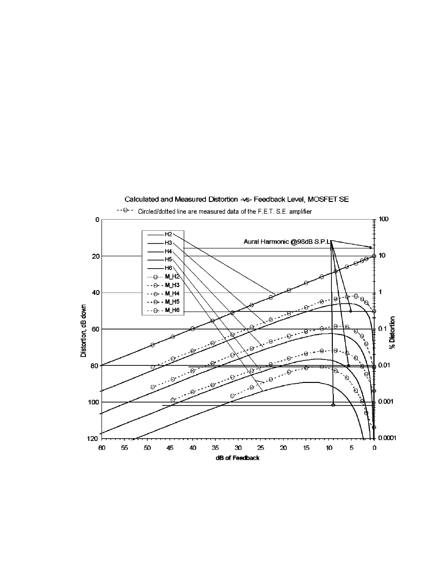
66
slight difference of the second harmonic. On interpreting the results for possible
masking by the ears aural harmonics the data gets interesting. Note in Fig. 3-2 the
additional horizontal lines marked “Aural Harmonic”. These represent the ear self
distortion at 98dB system S.P.L. Why plot 98dB? Because it is clear from the aural
harmonic envelope that the fall off matches most closely the zero-feedback data!
Fig. 3-2. Calculated and Measured Distortion versus feedback level, FET SE output
stage.
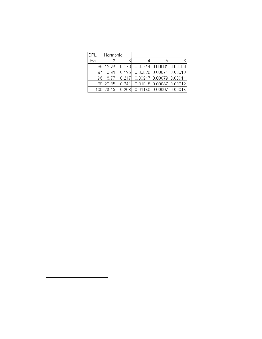
67
Table 3-1. Aural Harmonics from Eq. 2-1 over a reduced S.P.L range.
Table 3-1 is summarizes a range from 96 to 100dB SPL. The obvious interpretation is
that if feedback is believed to be required to reduce the subjectively benign 2
nd
harmonic,
even the slightest application pushes the harmonics together to an extent that aural
masking can never be complete. Or, on the other hand, if a large amount feedback is
instituted to reduce the harmonics to the levels without feedback, no single feedback
factor “fits” the aural harmonic envelope, and certainly, the H2 component will be so
reduced that masking is not in affect anyway. One may argue that I “made the data fit”
via plugging in a very high SPL. This is invalid, as the amplifier is sourcing the
equivalent of 2W, and, a 92 dB/W loudspeaker is commonplace, and a pair would, at 1
meter, create 98 dB S.P.L
32
.
A study, not as thorough as the FET SE gain stage, was done with two
different vacuum tubes. Both the type 19 and the type 45 showed a transfer characteristic
that was at least 5 times more linear than the FET over a much wider relative output
range (the a term was >5 times smaller). The type 19 is limited to 2/10W, and although
32
Most installation are two channel (stereo). 2W is 3dB louder than 1W, and two loudspeakers almost
double the S.P.L. 98-3-3 = 92dB

68
very promising musically, its dynamic range is audibly limited with normal efficiency
loudspeakers, to the extent that the reproduction seemed artificial because the level was
not as one experiences “live”. The type 45 with ~2.5W is indeed able to reach “jazz club”
signal levels with a 96dB/W loudspeaker system
33
. The harmonic content of a type 45
output stage was previously analyzed in Chapter 2 section 2, and plotted in Fig. 2-10. In
this amplifiers case, conformance to the aural harmonic envelope remained nearly exact
to 0.001% of fundamental.
2.
A Measurement protocol for the Total Aural Disconsonance figure of merit
In review, global or single stage negative feedback is not required for audio
amplification if a single-ended design is chosen. The design will contain harmonics at
much higher levels than the same device used in a feedback amplifier, but, the harmonics
may match the ears self-generated envelope of harmonics, and result in a better TAD
figure. In general only two gain stages will be required, in contrast to at least five with
modest feedback level amplifiers. TAD analysis is required on the whole amplifier,
including the driver / voltage gain stages. Commonly, there is very little power gain
required, and thus these stages are always more linear as the operating range is a smaller
portion of the devices total range. As discussed in Chapter 2 section 5, for TAD analysis
33
There exist larger triodes with similar symmetrical geometry to the type 45. For
example the type 50 is capable of greater than 6W but has reached such a cult status that
prices can reach over $500 for individual tubes at half-life discarded in the 30’s.
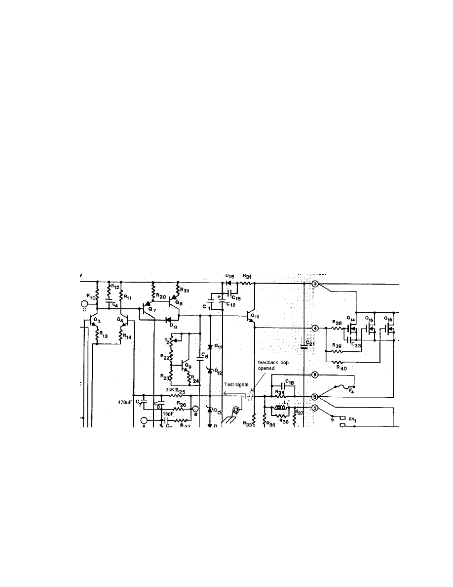
69
of feedback amplifiers, the feedback loop must be removed. In general the amplifier will
be unusable and probably stable as the gain is now increased by the feedback ratio,
usually 30dB or 1000 times.
In attempting testing of audio amplifiers with the feedback removed I
discovered a procedure that guarantees stability yet allows for the removal of the
feedback from the tested signal path. With the input left open, a low output impedance
signal in injected directly into the feedback path before the phase compensation network.
The output of the amplifier is now without the benefit of loop feedback and all the
following gain stages and the output stages are in a sense open loop. Fig. 3-3 shows the
Fig. 3.3. Subset of the DH500 amplifier schematic showing the point where feedback is
removed and a signal injected.
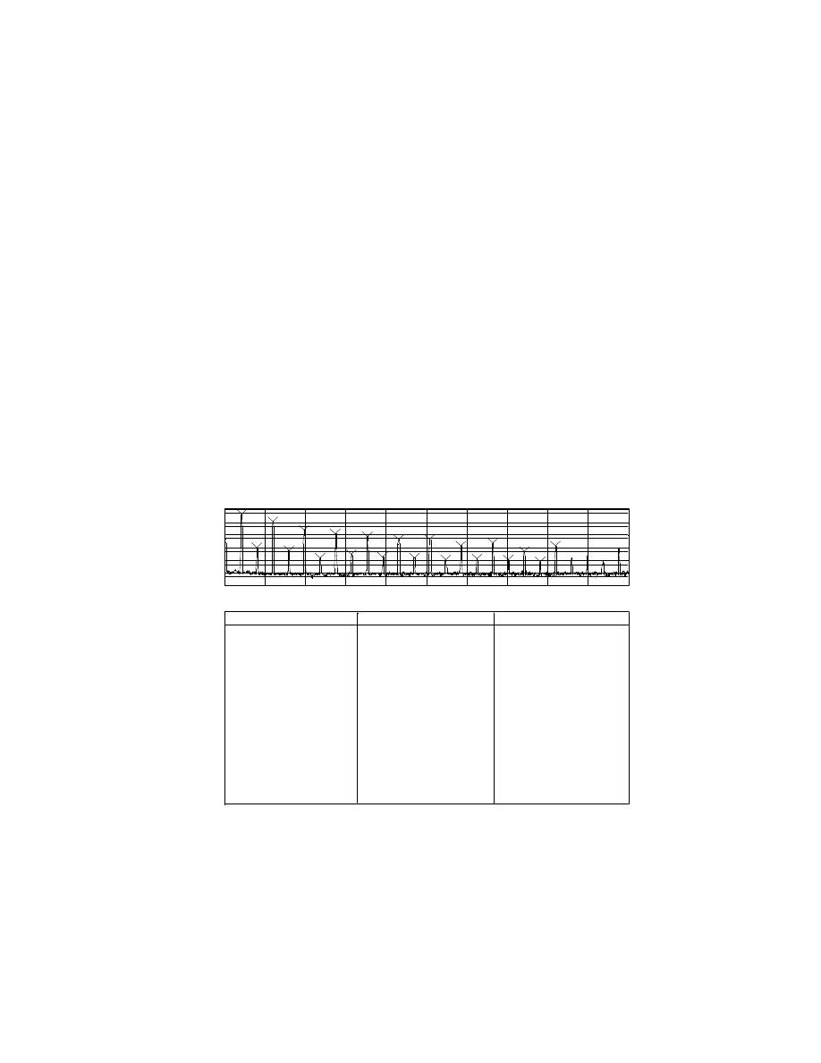
70
signal injection point for the DH500. Note the test signal source must be low output
impedance and be connected before the opening of the loop. This test signal runs through
the entire amplifier- Q3-Q7 diff. Amp, Q7-Q8 gain, and Q12 gate driver. The open loop
performance can now be tested with the same instrumentation. Harmonic distortion now
dominates. At 0.4W out ( similar output power as the type 45 amplifier shown in Fig.
1-16 ) the DH500 exhibited 23.6% THD, shown in the following Fig.3-4. Note the strong
odd-order components. These are not due to classic push-pull cross-over distortion, as the
DH500 bias circuit is connected and performing as designed, but must be due several
transistors in the forward path, but most likely the output FETs, swinging
0Hz
25.6kHz
AVG: 10
A:CH2 Pwr Spec
1
Vrms
1u
LogMag
6
decades
X:992 Hz
Y:450.864 mVrms
Entry Label
Hz
Vrms
Fundamental
1.008
k
450.812
m
2nd
2
k
853.673
u
3rd
3.008
k
102.414
m
4th
4
k
542.8
u
5th
5.008
k
24.776
m
6th
6
k
149.32
u
7th
7.008
k
11.117
m
8th
8
k
281.112
u
9th
9.008
k
7.288
m
10th
10.016
k
165.057
u
11th
11.008
k
4.151
m
12th
12.016
k
139.881
u
13th
13.008
k
4.092
m
14th
14.016
k
101.015
u
15th
15.008
k
1.275
m
B:CH2 Pwr Spec
AVG: 10
LogMag
THD:23.6032 %
Fig. 3-4. DH500 Open-loop harmonic distortion at 0.4W

71
into a non-linear area. These harmonics needless to say do not follow the aural harmonic
envelope. Calculation of the TAD is not necessary. The claim is that this poor open-loop
performance is why the amplifier did not sound as natural or dynamic as the type 45 tube
amplifier.

72
CONCLUSION
The research I undertook to determine a better audio amplifier measurement
methodology has resulted in a concept and method that better correlates an objective
figure of merit to the subjective experience than previous protocols. Rudimentary
exploration with a varied listening panel of five people using directly fed real-time
signals from a piano showed that the T.A.D. number rated a set of 3 amplifiers correctly
while the standard accepted T.H.D. and I.M. results did not. It is my belief that the TAD
figure of merit specification, in general, applied to a broader set of electronic devices,
enables objective measurements to better rate sound reproduction equipment sound
quality. Those who have the intent to consider further research in this area could
concentrate on the following areas:
•
T.A.D. system effects. Even the very well designed loudspeaker is the highest
distorting device in the audio chain. The harmonics fall off sharply with rising
order on the other hand. Perhaps the system T.A.D. actually correlates better with
the natural harmonic envelope of the ear with the addition of the >5% 2
nd
harmonic distortion of the loudspeaker.
•
T.A.D. of the storage and retrieval system. Perhaps lowering the T.A.D. rating of
digital electronics by concentration on bit depth rather than raising the channel

73
density (surround sound) or the sampling rate can result in real gains in
transparency.
•
Sex and age effects on an individuals aural harmonic envelope. Similar studies to
the Fletcher and Olson aural harmonics work can be carried out to determine any
major changes in the harmonic envelope.
The limitations of the research documented herein are similar to the
previous statements. The aural harmonic envelope needs to be proven reasonably
similar acroos age, sex, and other factors in order for the T.A.D. mathematical
derivation to be accurate. The entire sound reproduction system is required to follow
the harmonic envelope. It is my belief that the audio power amplifier is the largest
detractor from the envelope, but this needs to be proven.
The public has limited access to participate in demonstrations of single-
ended audio amplifiers. Very few mainstream Hi-Fi shops have this type of
equipment set-up. I know of none in the Boston area. If the reason for this is the need
for suppliers and salespeople to stick to what they know- mainly the specifications
race then the specifications need to change. These amplifiers are clearly superior in
many of the most important areas of sound reproduction. Unfortunately the design
has some drawbacks.
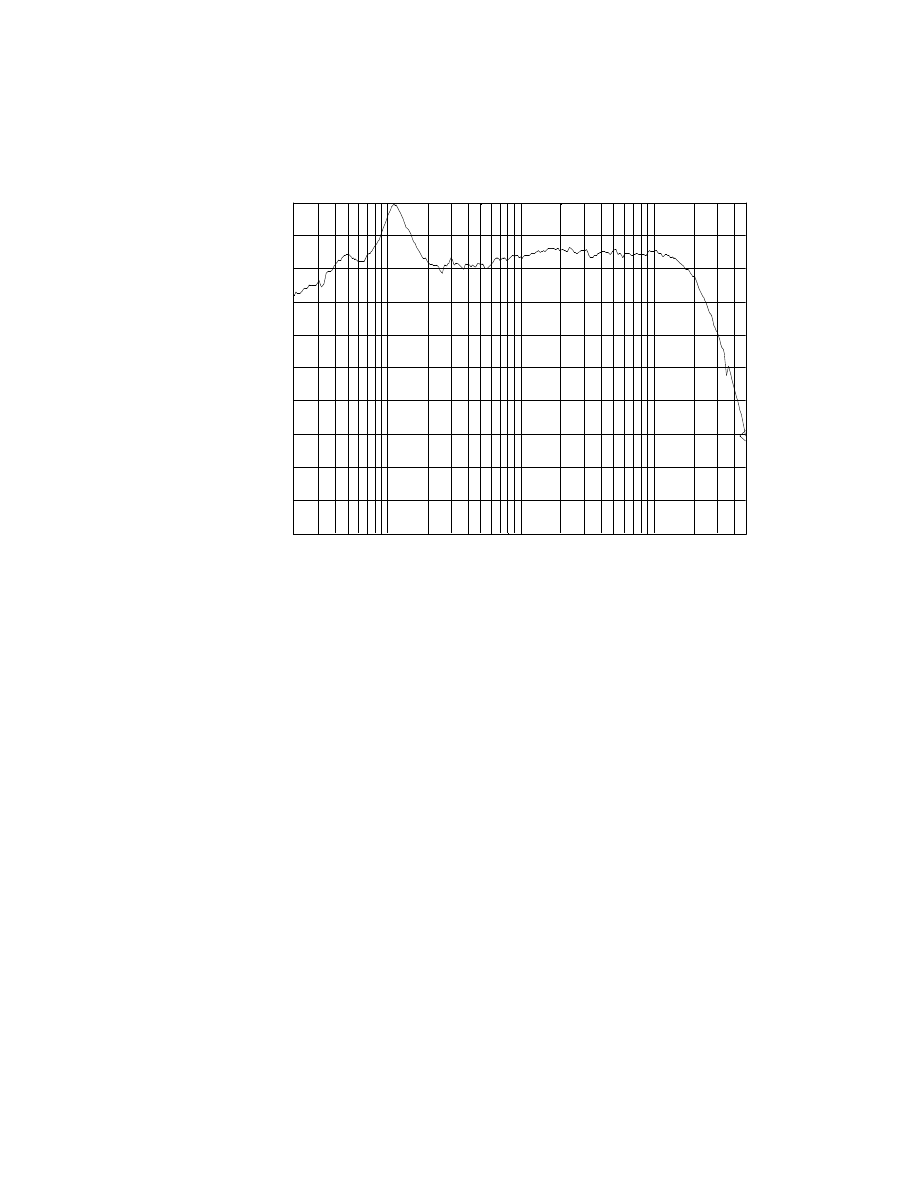
74
B:CH2 Lin Spec X:50 kHz
Y:-3.4555 dBVrms
20Hz
50kHz
3.6
dBVrms
-6.4
dBVrms
dB Mag
1
dB
/div
Fig. 3-5. Output level variation of the type 45 SE amplifier when loaded with a
loudspeaker
The output impedance of these amplifiers is in the ohms range, hundreds of times worse
than solid-state push-pull amplifiers. This requires careful mating with loudspeakers that
do not have great impedance variation with frequency. For example, a set of 1960’s
Radio Shack 16 ohm PA monitors was necessarily chosen in the listening tests because it
had a very little impedance variation over the range of frequencies used in the listening
tests- a grand piano. As shown in Fig 3-5, this speaker was flat within +/- 0.25dB from
180Hz to 18kHz, meeting the ABX
[40]
specifications for frequency response matching.
Loudspeaker efficiency is also an issue with amplifiers with power outputs of less than
5W. This is being addressed and there are dozens of loudspeakers on the market with

75
efficiencies greater that 95dB/W/m. The plusses far outweigh the minuses and I am
convinced that zero-feedback single-ended designs will continue to become more
widespread. I plan on pursuing this methodology, and am in the process of designing a
PC based data-acquisition system that displays real time TAD figures, allowing for the
fine tuning of bias points in audio amplifiers.

76
BIBLIOGRAPHY
[1]
Stereophile Magazine. Vol. 18 No. 9, September 1995 pp. 141-149
Stereophile, 208 Delgado, Santa Fe, NM 87501
[2]
Stereophile Magazine. Vol. 18 No. 9, September 1995 p.145
[3]
Stereophile Magazine. Vol. 18 No. 9, September 1995 p. 148
[4]
Stereophile Magazine. Vol. 18 No. 9, September 1995 pp. 147-148
[5]
Stereophile Magazine. Vol. 198 No. 10, October 1996 p.284
[6]
Kellogg, Edward. “The design of non-distorting power amplifiers”
[7]
W.T. Cocking 1934
[8]
Black, Harold S. “Stabilized Feedback Amplifiers”
BSTJ January 1934, pp. 1-18
[9]
Williamson, D.T.N., “Design for a High Quality Amplifier”
Wireless World, April 1947 (pt1) pp. 118-121;
May 1947(pt2), pp. 161-163.
[10]
McIntosh, Frank & Gow, Gordon. “ Description and Analysis of a New 50-Watt
Amplifier Circuit”
Audio Engineering, December1949
[11]
Hafler, David & Keroes, Herbert. “An Ultra-Linear Amplifier”
Audio Engineering, June 1952
[12]
Radio Manufacturers Association (UK) 1937 “Specification for testing and
expressing overall performance of radio broadcast receivers”
[13]
Callendar, M.V “Feedback” column
Electrical Engineering, October 1950 p. 443

77
[14] Shorter, D.E.L. “The Influence of High Order Products in Non-Linear
Distortion”
Electrical Engineering, April 1950 pp.152-153
[15]
Bloch, Alan “Measurement of Non Linear Distortion”
Journal of the Audio Engineering Society, January 1953 pp. 62-67
[16] SMPTE I.M. Standard
“Society for Motion Picture and Television Engineers”
[17]
Crowhearst, Norman. “Some Defects in Amplifier Performance not covered by
Standard Specifications”
Journal of the Audio Engineering Society, October 1957. pp. 195-201
[18]
Crowhearst, Norman. “Feedback – Head Cook and Bottle Washer”
Audio, April 1959
[19]
Listener Magazine, Vol 7, No.5 (9,10 2001) pp. 62. ISSN number 1529-9333
Englander Communications, LLC, 75 Holly Hill Lane, Greenwich, CT 06830
[20]
Otala, Mati J. “Transient Distortion in Transistor Audio Power Amplifiers”
Journal of the Audio Engineering Society, 1970
[21]
Otala, Mati J. “Circuit Design Modifications for Minimizing Transient
Intermodulation Distortion in Transistor Audio Power Amplifiers”
Journal of the Audio Engineering Society, 1977
[22]
Otala, Mati J. “A Method for Measuring T.I.M.”
Journal of the Audio Engineering Society, 1977
[23] Otala, Mati J. “Correlation Audio Distortion Measurements”
Journal of the Audio Engineering Society, Jan/Feb 1978, Vol. 26 No. 12
pp. 12-19
[24] Cabot, Richard C. “Comparison of Nonlinear Distortion Measurement Methods”
Proceedings of the 11
th
International AES Conference 1992.
[25] Pass, Nelson. Article “Single ended class A”
http://www.passlabs.com/articles/seclassa.htm

78
[26]
Stereophile Magazine. Vol. 21 No. 3, March 1998 p. 148
[27]
M. Liberman, "Cochlear Frequency Map for the Cat",
Acoust. Society of America. pp72-77, Nov. 1982.
[28]
Olsen, Harry F. “Music, Physics and Engineering”
Dover Publications, Inc. N.Y., 2nd ed. : 1967.
[29] Newman, Edwin Broomell..”Factors in the production of aural harmonics and
combination tones” Lancaster, Pa., Lancaster Press, 1937.
Reprinted from The Journal of the Acoustical Society of America, Vol. 9, No. 2,
October, 1937.
[30] , [31] , [32]
Fletcher “Speech and Hearing”, 1924.
D.Van Nostrand Company, Inc, and Bell Telephone Laboratories.
[33] , [34]
Olson, Harry F. , Massa, Frank. F. “Applied Acoustics”, 1934
Van Nostrand Co.
[35] J. Goldstein, "Auditory Non-linearity", J. Acoustical Society of America. 41, pp.
676-689, 1967
[36] Alternatively, the ear generates intermodulation products due to the same non-
linearity that causes Aural Harmonics to appear
[37] Roerderer, Juan G. “Introduction to the Physics and Phychophysics of Music” 2
nd
Edition. 1979.
Heidelberg Science Library, Spring-Verlag, Berlin Germany
[38] Northrop, Robert B. “Analog Electronic Circuits”
Addison-Welsley 1990
[39] LM3886 data sheet. National Semiconductor Corporation
http://ww.national.com/datasheets/lm3886.pdf

79
[40] Clark, David L., "High-Resolution Subjective Testing Using a Double-Blind
Comparator", Journal of the Audio Engineering Society, Vol. 30 No. 5, May
1982, pp. 330-338.
Wyszukiwarka
Podobne podstrony:
Data Mining Methods for Detection of New Malicious Executables
A new evaluation method for lumbar spinal instability
Guidelines For Measuring Audio Power Amplifier Performance (Texas Instruments)
A New Rapid Method for Detecting Val103Ile
New technologies for cervical cancer screening
BP4078 Class D Audio Power Amplifier
Free Energy Bedini Device And Method For Pulse Charging A Battery Patent Info 2004
Fibonacci Practical Fibonacci Methode For Forex Trading
Improvements in Fan Performance Rating Methods for Air and Sound
Zied H A A modular IGBT converter system for high frequency induction heating applications
58 829 845 A New Model for Fatique Failure due to Carbide Clusters
14 175 184 DE GP4M a New Generation for Tool Steel Casting
Combinatorial Methods for Polymer Science
Bradykinin B2 receptor antagonism a new direction for acute stroke therapy
Metallographic Methods for Revealing the Multiphase Microstructure of TRIP Assisted Steels TŁUMA
de BROIN F & alii 2008 Eurotestudo, a new genus for the species Testudo hermanni
Methodology for Assessment Biodiversity
FOREX Systems Research Practical Fibonacci Methods For Forex Trading 2005
Numerical Methods for Engineers and Scientists, 2nd Edition
więcej podobnych podstron