
© 2006 ANSYS, Inc. All rights reserved.
ANSYS, Inc. Proprietary
Solver Settings
Solver Settings
Introductory FLUENT Training
Introductory FLUENT Training

5-2
© 2006 ANSYS, Inc. All rights reserved.
ANSYS, Inc. Proprietary
Fluent User Services Center
www.fluentusers.com
Introductory FLUENT Notes
FLUENT v6.3 December 2006
Outline
Using the Solver
z
Setting Solver Parameters
z
Convergence
Definition
Monitoring
Stability
Accelerating Convergence
z
Accuracy
Grid Independence
Grid Adaption
z
Unsteady Flows Modeling
Unsteady-flow problem setup
Unsteady flow modeling options
z
Summary
z
Appendix

5-3
© 2006 ANSYS, Inc. All rights reserved.
ANSYS, Inc. Proprietary
Fluent User Services Center
www.fluentusers.com
Introductory FLUENT Notes
FLUENT v6.3 December 2006
Outline
Using the Solver (solution procedure overview)
z
Setting Solver Parameters
z
Convergence
Definition
Monitoring
Stability
Accelerating Convergence
z
Accuracy
Grid Independence
Grid Adaption
z
Unsteady Flows Modeling
Unsteady-flow problem setup
Unsteady flow modeling options
z
Summary
z
Appendix
5-4
© 2006 ANSYS, Inc. All rights reserved.
ANSYS, Inc. Proprietary
Fluent User Services Center
www.fluentusers.com
Introductory FLUENT Notes
FLUENT v6.3 December 2006
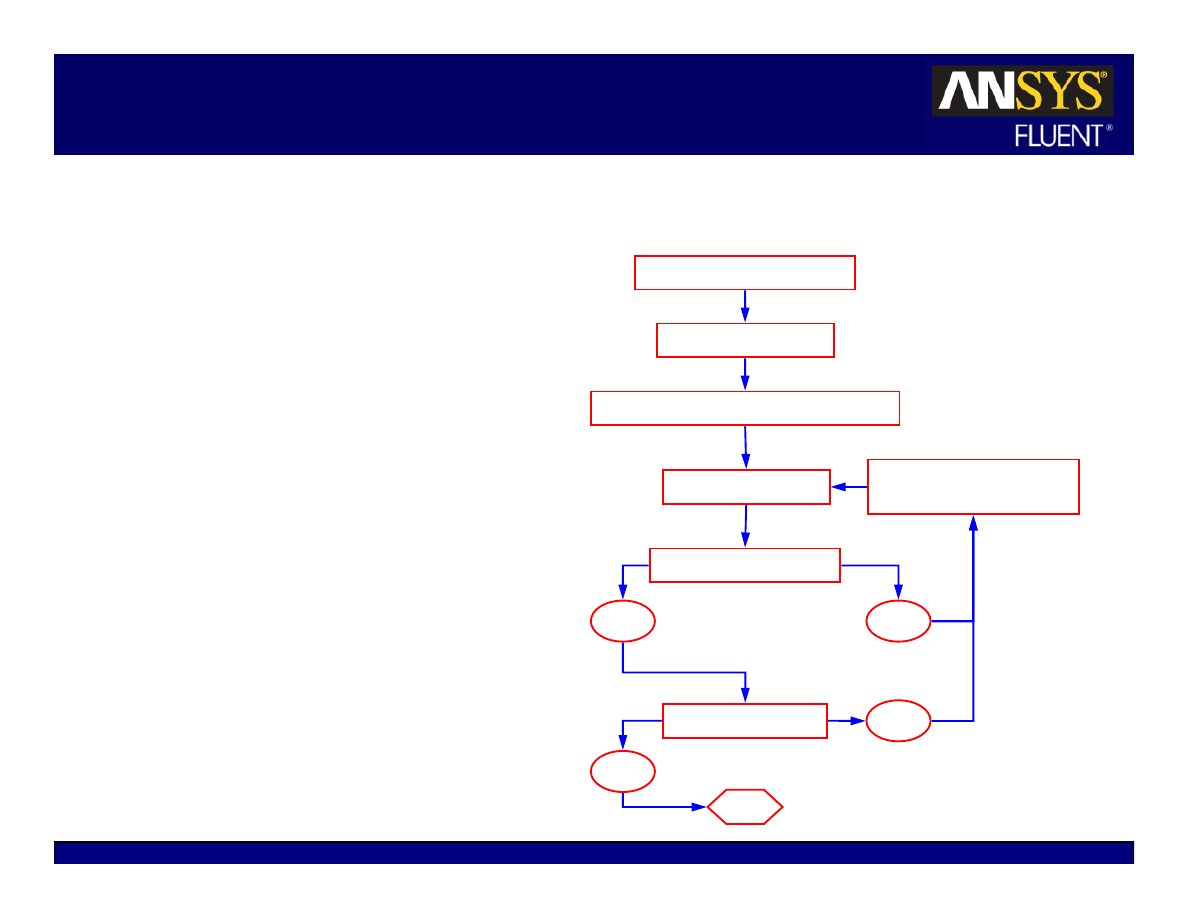
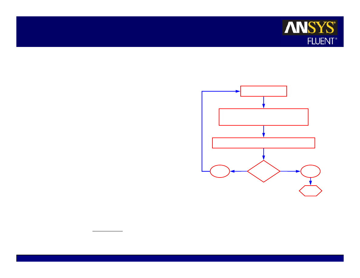
No
Set the solution parameters
Initialize the solution
Enable the solution monitors of interest
Modify solution
parameters or grid
Calculate a solution
Check for convergence
Check for accuracy
Stop
Solution Procedure Overview
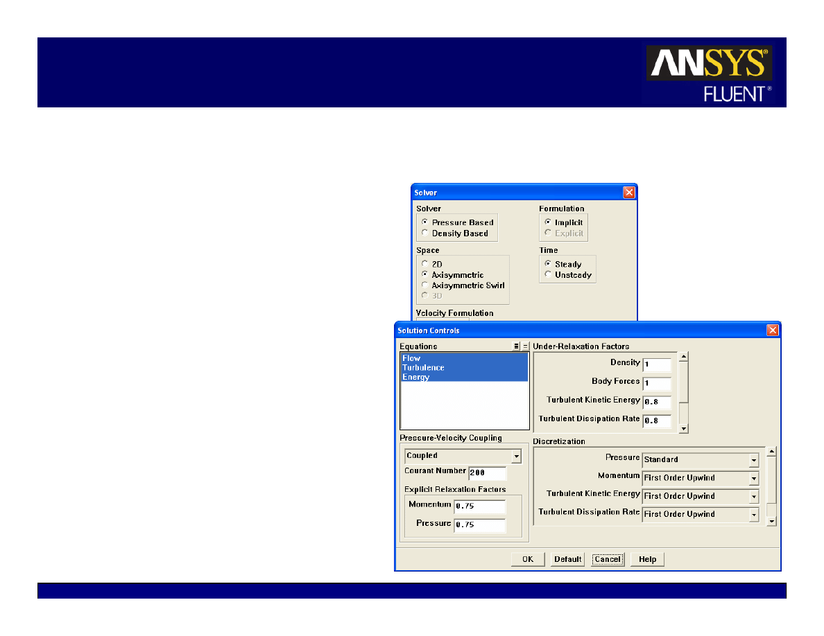
Solution parameters
z
Choosing the solver
z
Discretization schemes
Initialization
Convergence
z
Monitoring convergence
z
Stability
Setting Under-relaxation
Setting Courant number
z
Accelerating convergence
Accuracy
z
Grid Independence
z
Adaption
Yes
Yes
No
5-5
© 2006 ANSYS, Inc. All rights reserved.
ANSYS, Inc. Proprietary
Fluent User Services Center
www.fluentusers.com
Introductory FLUENT Notes
FLUENT v6.3 December 2006
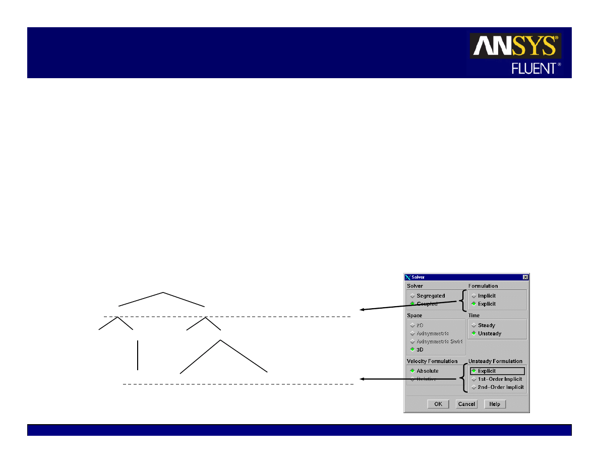
Available Solvers
There are two kinds of solvers available in
FLUENT.
z
Pressure-based solver
z
Density-based coupled solver (DBCS)
The
pressure-based
solvers take momentum
and pressure (or pressure correction) as the
primary variables.
Pressure-velocity coupling algorithms are
derived by reformatting the continuity
equation
Two algorithms are available with the
pressure-based solvers:
z
Segregated solver – Solves for pressure
correction and momentum sequentially.
z
Coupled Solver (PBCS) – Solves pressure and
momentum simultaneously.
Segregated
PBCS
Solve Turbulence Equation(s)
Solve Species
Solve Energy
DBCS
Solve Other Transport Equations as required
Solve Mass
Continuity;
Update Velocity
Solve U-Momentum
Solve V-Momentum
Solve W-Momentum
Solve Mass
& Momentum
Solve Mass,
Momentum,
Energy,
Species
5-6
© 2006 ANSYS, Inc. All rights reserved.
ANSYS, Inc. Proprietary
Fluent User Services Center
www.fluentusers.com
Introductory FLUENT Notes
FLUENT v6.3 December 2006
Available Solvers
Density-Based Coupled Solver
–
equations for continuity, momentum,
energy, and species, if required, are
solved in vector form. Pressure is
obtained through the equation of state.
Additional scalar equations are solved
in a segregated fashion.
The density-based solver can use
either an implicit or explicit solution
approach:
z
Implicit – Uses a point-implicit Gauss-
Seidel / symmetric block Gauss-Seidel
/ ILU method to solve for variables.
z
Explicit: uses a multi-step Runge-
Kutta explicit time integration method
Note:
the pressure-based solvers are
implicit

5-7
© 2006 ANSYS, Inc. All rights reserved.
ANSYS, Inc. Proprietary
Fluent User Services Center
www.fluentusers.com
Introductory FLUENT Notes
FLUENT v6.3 December 2006
Choosing a Solver
The
pressure-based
solver is applicable for a wide range of flow regimes from
low speed incompressible flow to high-speed compressible flow.
z
Requires less memory (storage).
z
Allows flexibility in the solution procedure.
The
pressure-based
coupled solver (PBCS) is applicable for most single phase
flows, and yields superior performance to the
pressure-based
(segregated)
solver.
z
Not available for multiphase (Eulerian), periodic mass-flow and NITA cases.
z
Requires 1.5–2 times more memory than the segregated solver.
The
density-based
coupled solver (DBCS) is applicable when there is a strong
coupling, or interdependence, between density, energy, momentum, and/or
species.
z
Examples: High speed compressible flow with combustion, hypersonic flows,
shock interactions.
The Implicit solution approach is generally preferred to the explicit approach,
which has a very strict limit on time step size
The explicit approach is used for cases where the characteristic time scale of
the flow is on the same order as the acoustic time scale. (e.g.: propagation of
high-Ma shock waves).
5-8
© 2006 ANSYS, Inc. All rights reserved.
ANSYS, Inc. Proprietary
Fluent User Services Center
www.fluentusers.com
Introductory FLUENT Notes
FLUENT v6.3 December 2006
Discretization (Interpolation Methods)
Field variables (stored at cell centers) must be interpolated to the faces of the
control volumes.
Interpolation schemes for the convection term:
z
First-Order Upwind
– Easiest to converge, only first-order accurate.
z
Power Law
– More accurate than first-order for flows when Re
cell
< 5 (typ. low Re
flows)
z
Second-Order Upwind
– Uses larger stencils for 2nd order accuracy, essential with
tri/tet mesh or when flow is not aligned with grid; convergence may be slower.
z
Monotone Upstream-Centered Schemes for Conservation Laws (MUSCL)
–
Locally 3rd order convection discretization scheme for unstructured meshes; more
accurate in predicting secondary flows, vortices, forces, etc.
z
Quadratic Upwind Interpolation (QUICK)
– Applies to quad/hex and hybrid
meshes, useful for rotating/swirling flows, 3rd-order accurate on uniform mesh
( )
V
S
V
t
N
f
f
f
N
f
f
f
f
f
φ
φ
+
⋅
φ
∇
Γ
=
⋅
φ
ρ
+
∂
ρφ
∂
∑
∑
faces
faces
A
A
V
5-9
© 2006 ANSYS, Inc. All rights reserved.
ANSYS, Inc. Proprietary
Fluent User Services Center
www.fluentusers.com
Introductory FLUENT Notes
FLUENT v6.3 December 2006
Interpolation Methods (Gradients)
Gradients of solution variables are required in order to evaluate
diffusive fluxes, velocity derivatives, and for higher-order
discretization schemes.
The gradients of solution variables at cell centers can be determined
using three approaches:
z
Green-Gauss Cell-Based
– The default method; solution may have false
diffusion (smearing of the solution fields).
z
Green-Gauss Node-Based
– More accurate; minimizes false diffusion;
recommended for tri/tet meshes.
z
Least-Squares Cell-Based
– Recommended for polyhedral meshes; has the
same accuracy and properties as Node-based Gradients.
Gradients of solution variables at faces computed using multi-
dimensional Taylor series expansion
( )
V
S
V
t
N
f
f
f
N
f
f
f
f
f
φ
φ
+
⋅
φ
∇
Γ
=
⋅
φ
ρ
+
∂
ρφ
∂
∑
∑
faces
faces
A
A
V

5-10
© 2006 ANSYS, Inc. All rights reserved.
ANSYS, Inc. Proprietary
Fluent User Services Center
www.fluentusers.com
Introductory FLUENT Notes
FLUENT v6.3 December 2006
Interpolation Methods for Face Pressure
Interpolation schemes for calculating cell-face pressures when using
the segregated solver in FLUENT are available as follows:
z
Standard
– The default scheme; reduced accuracy for flows exhibiting
large surface-normal pressure gradients near boundaries (but should not be
used when steep pressure changes are present in the flow – PRESTO!
scheme should be used instead.)
z
PRESTO!
– Use for highly swirling flows, flows involving steep pressure
gradients (porous media, fan model, etc.), or in strongly curved domains
z
Linear
– Use when other options result in convergence difficulties or
unphysical behavior
z
Second-Order
– Use for compressible flows; not to be used with porous
media, jump, fans, etc. or VOF/Mixture multiphase models
z
Body Force Weighted
– Use when body forces are large, e.g., high Ra
natural convection or highly swirling flows

5-11
© 2006 ANSYS, Inc. All rights reserved.
ANSYS, Inc. Proprietary
Fluent User Services Center
www.fluentusers.com
Introductory FLUENT Notes
FLUENT v6.3 December 2006
Pressure-Velocity Coupling
Pressure-velocity coupling refers to the numerical algorithm which
uses a combination of continuity and momentum equations to derive
an equation for pressure (or pressure correction) when using the
pressure-based solver.
Four algorithms are available in FLUENT.
z
Semi-Implicit Method for Pressure-Linked Equations (SIMPLE)
The default scheme, robust
z
SIMPLE-Consistent (SIMPLEC)
Allows faster convergence for simple problems (e.g., laminar flows with
no physical models employed).
z
Pressure-Implicit with Splitting of Operators (PISO)
Useful for unsteady flow problems or for meshes containing cells with
higher than average skewness
z
Fractional Step Method (FSM)
for unsteady flows.
Used with the NITA scheme; similar characteristics as PISO.
5-12
© 2006 ANSYS, Inc. All rights reserved.
ANSYS, Inc. Proprietary
Fluent User Services Center
www.fluentusers.com
Introductory FLUENT Notes
FLUENT v6.3 December 2006
Initialization
Iterative procedure requires that all
solution variables be initialized before
calculating a solution
z
Realistic guesses improves solution
stability and accelerates convergence
z
In some cases, a good initial guess is
required.
Example: high temperature region to
initiate chemical reaction.
Patch values for individual variables
in certain regions.
z
Free jet flows (high velocity for jet)
z
Combustion problems (high temperature
region to initialize reaction)
z
Cell registers (created by marking the
cells in the Adaption panel) can be used
for patching values into various regions
of the domain.
Solve
Initialize
Initialize…
Solve
Initialize
Patch…

5-13
© 2006 ANSYS, Inc. All rights reserved.
ANSYS, Inc. Proprietary
Fluent User Services Center
www.fluentusers.com
Introductory FLUENT Notes
FLUENT v6.3 December 2006
FMG Initialization
Full Multigrid (FMG) Initialization can be used to create a better initialization
of the flow field:
z
TUI command:
/solve/init/fmg-initialization
FMG is computationally inexpensive and faster. Euler equations are solved
with first-order accuracy on the coarse-level meshes.
It can be used with both pressure and density based solvers, but only in steady
state.
FMG uses the Full Approximation Storage (FAS) multigrid method to solve
the flow problem on a sequence of coarser meshes, before transferring the
solution onto the actual mesh.
z
Settings can be accessed by the TUI command:
/solve/init/set-fmg-initialization
FMG Initialization is useful for complex flow problems involving large
gradients in pressure and velocity on large domains (e.g.: rotating machinery,
expanding spiral ducts)
5-14
© 2006 ANSYS, Inc. All rights reserved.
ANSYS, Inc. Proprietary
Fluent User Services Center
www.fluentusers.com
Introductory FLUENT Notes
FLUENT v6.3 December 2006
Case Check
Case Check is a utility in FLUENT which looks for common setup errors and
provides guidance in selecting case parameters and models.
z
Uses rules and best practices
Case check will look for compliance in:
z
Grid
z
Model Selection
z
Boundary Conditions
z
Material Properties
z
Solver Settings
Tabbed sections contain
recommendations
Automatic recommendations:
the utility will make the changes
Manual recommendations: the
user has to make the changes
Solve
Case Check…

5-15
© 2006 ANSYS, Inc. All rights reserved.
ANSYS, Inc. Proprietary
Fluent User Services Center
www.fluentusers.com
Introductory FLUENT Notes
FLUENT v6.3 December 2006
Outline
Using the Solver
z
Setting Solver Parameters
z
Convergence
Definition
Monitoring
Stability
Accelerating Convergence
z
Accuracy
Grid Independence
Grid Adaption
z
Unsteady Flows Modeling
Unsteady-flow problem setup
Unsteady flow modeling options
z
Summary
z
Appendix

5-16
© 2006 ANSYS, Inc. All rights reserved.
ANSYS, Inc. Proprietary
Fluent User Services Center
www.fluentusers.com
Introductory FLUENT Notes
FLUENT v6.3 December 2006
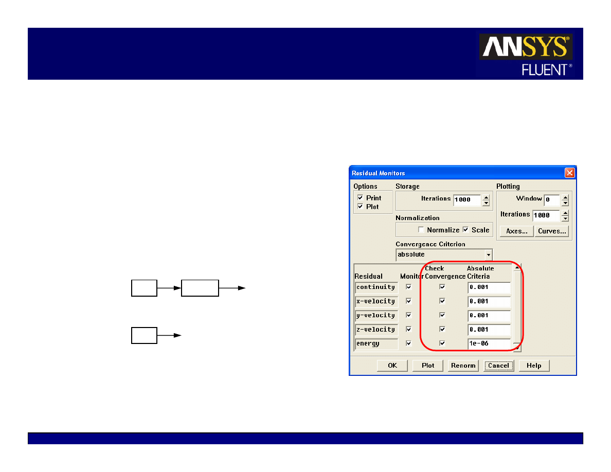
Convergence
At convergence, the following should be satisfied:
z
All discrete conservation equations (momentum, energy, etc.) are obeyed in all
cells
to a specified tolerance
OR the solution no longer changes with subsequent
iterations.
z
Overall mass, momentum, energy, and scalar balances are achieved.
Monitoring convergence using residual history:
z
Generally, a decrease in residuals by
three orders of magnitude
indicates at least
qualitative convergence. At this point, the major flow features should be
established.
z
Scaled energy residual must decrease to 10
-6
(for the pressure-based solver).
z
Scaled species residual may need to decrease to 10
-5
to achieve species balance.
Monitoring quantitative convergence:
z
Monitor other relevant key variables/physical quantities for a confirmation.
z
Ensure that overall mass/heat/species conservation is satisfied.
5-17
© 2006 ANSYS, Inc. All rights reserved.
ANSYS, Inc. Proprietary
Fluent User Services Center
www.fluentusers.com
Introductory FLUENT Notes
FLUENT v6.3 December 2006
Convergence Monitors: Residuals
Residual plots show when the residual values have reached the
specified tolerance.
All equations converged.
10
-3
10
-6
Solve
Monitors
Residual…
5-18
© 2006 ANSYS, Inc. All rights reserved.
ANSYS, Inc. Proprietary
Fluent User Services Center
www.fluentusers.com
Introductory FLUENT Notes
FLUENT v6.3 December 2006
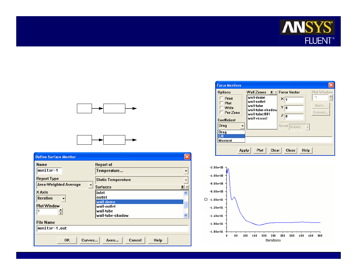
Convergence Monitors: Forces/Surfaces
In addition to residuals, you can also monitor:
z
Lift, drag, or moment
z
Pertinent variables or functions (e.g., surface
integrals) at a boundary or any defined surface.
Solve
Monitors
Force…
Solve
Monitors
Surface…
5-19
© 2006 ANSYS, Inc. All rights reserved.
ANSYS, Inc. Proprietary
Fluent User Services Center
www.fluentusers.com
Introductory FLUENT Notes
FLUENT v6.3 December 2006
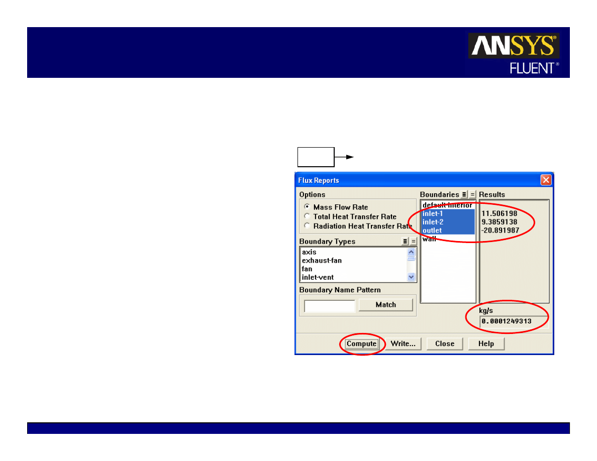
Checking for Flux Conservation
In addition to monitoring
residual and variable histories,
you should also check for
overall heat and mass
balances.
The net imbalance should be
less than 1% of the smallest
flux through the domain
boundary
Report
Fluxes…
5-20
© 2006 ANSYS, Inc. All rights reserved.
ANSYS, Inc. Proprietary
Fluent User Services Center
www.fluentusers.com
Introductory FLUENT Notes
FLUENT v6.3 December 2006
Tightening the Convergence Tolerance
If solution monitors indicate that the
solution is converged, but the solution is
still changing or has a large mass/heat
imbalance, this clearly indicates the solution
is not yet converged.
In this case, you need to:
z
Reduce values of Convergence Criterion
or disable Check Convergence in the Residual
Monitors panel.
z
Continue iterations until the solution
converges.
Selecting none under Convergence Criterion
will instruct FLUENT to not check
convergence for any equations.
Solve
Monitors
Solve
Iterate…
Residual…
5-21
© 2006 ANSYS, Inc. All rights reserved.
ANSYS, Inc. Proprietary
Fluent User Services Center
www.fluentusers.com
Introductory FLUENT Notes
FLUENT v6.3 December 2006
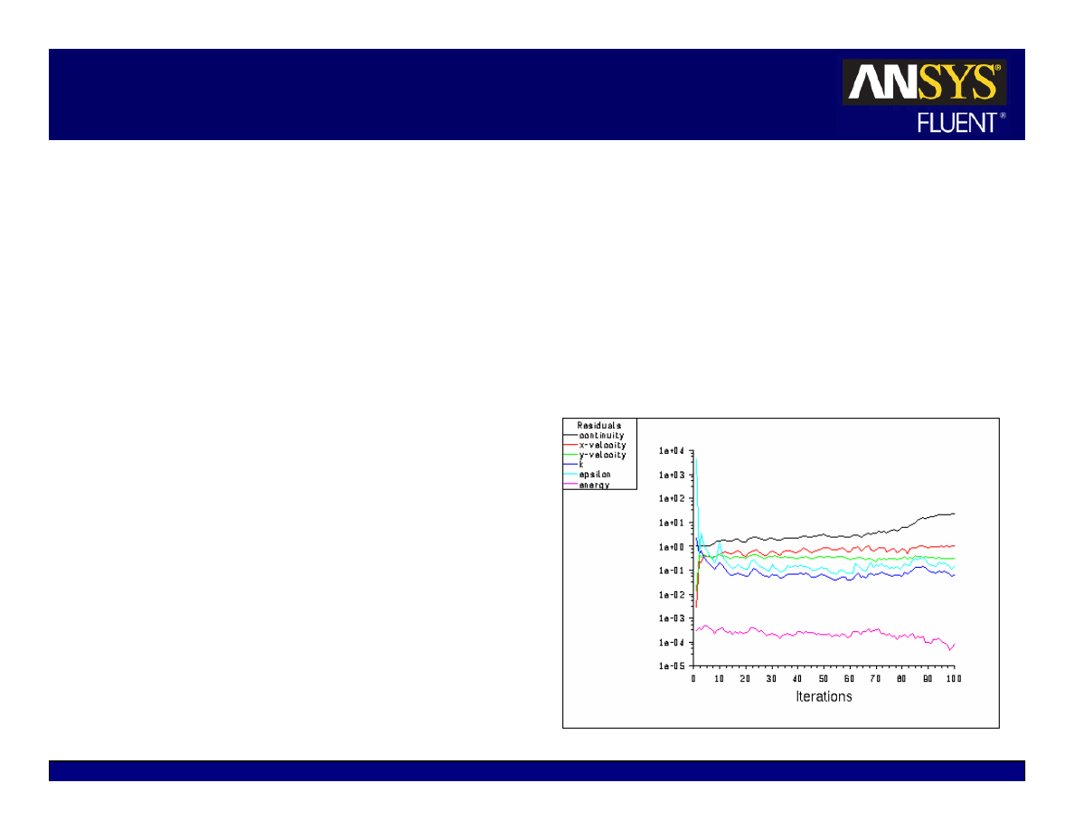
Convergence Difficulties
Numerical instabilities can arise with an ill-posed problem, poor quality mesh,
and/or inappropriate solver settings.
z
Exhibited as increasing (diverging) or “stuck” residuals.
z
Diverging residuals imply increasing imbalance in conservation equations.
z
Unconverged results are very misleading!
Continuity equation convergence
trouble affects convergence of
all equations.
Troubleshooting
z
Ensure that the problem is well-
posed.
z
Compute an initial solution using a
first-order discretization scheme.
z
Decrease under-relaxation factors for
equations having convergence
problems (pressure-based solver).
z
Decrease the Courant number
(density-based solver)
z
Remesh or refine cells which have
large aspect ratio or large skewness.
5-22
© 2006 ANSYS, Inc. All rights reserved.
ANSYS, Inc. Proprietary
Fluent User Services Center
www.fluentusers.com
Introductory FLUENT Notes
FLUENT v6.3 December 2006
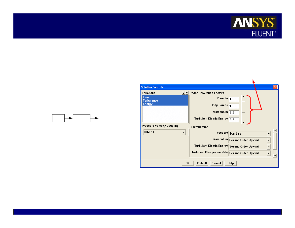
Modifying Under-Relaxation Factors
Under-relaxation factor,
α, is
included to stabilize the iterative
process for the pressure-based
solver
Use default under-relaxation
factors to start a calculation.
Decreasing under-relaxation for
momentum often aids
convergence.
z
Default settings are suitable for a
wide range of problems, you can
reduce the values when necessary
z
Appropriate settings are best
learned from experience!
p
p
p
φ
∆
α
+
φ
=
φ
old
,
For density-based solvers, under-relaxation factors for equations outside
coupled set are modified as in the pressure-based solver.
Solve
Controls
Solution…
5-23
© 2006 ANSYS, Inc. All rights reserved.
ANSYS, Inc. Proprietary
Fluent User Services Center
www.fluentusers.com
Introductory FLUENT Notes
FLUENT v6.3 December 2006
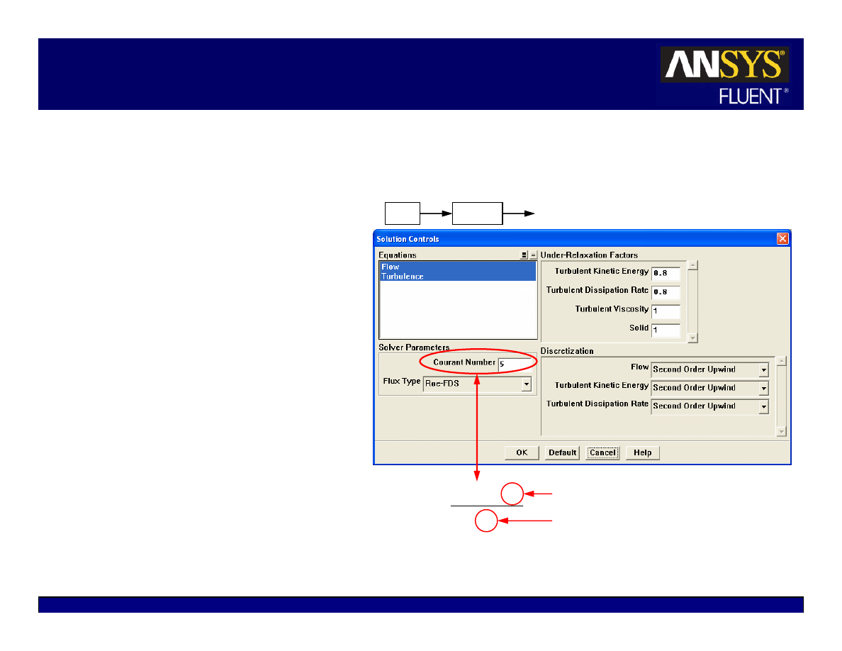
Modifying the Courant Number
A transient term is included in the
density-based solver even for
steady state problems.
z
The Courant number defines the
time step size.
For density-based explicit solver:
z
Stability constraints impose a
maximum limit on the Courant
number.
Cannot be greater than 2
(default value is 1).
Reduce the Courant number
when having difficulty
converging.
For density-based implicit solver:
z
The Courant number is not limited
by stability constraints.
Default value is 5.
u
x
t
∆
=
∆
)
CFL
(
Solve
Controls
Solution…
Mesh size
Appropriate velocity scale

5-24
© 2006 ANSYS, Inc. All rights reserved.
ANSYS, Inc. Proprietary
Fluent User Services Center
www.fluentusers.com
Introductory FLUENT Notes
FLUENT v6.3 December 2006
Accelerating Convergence
Convergence can be accelerated by:
z
Supplying better initial conditions
Starting from a previous solution (using file/interpolation when necessary)
z
Gradually increasing under-relaxation factors or Courant number
Excessively high values can lead to instabilities or convergence problems
Recommend saving case and data files before continuing iterations
z
Controlling multigrid solver settings (but default settings provide a robust
Multigrid setup and typically do not need to be changed). See the
Appendix for details on the Multigrid settings.
5-25
© 2006 ANSYS, Inc. All rights reserved.
ANSYS, Inc. Proprietary
Fluent User Services Center
www.fluentusers.com
Introductory FLUENT Notes
FLUENT v6.3 December 2006
Starting from a Previous Solution
Previous solution can be used as an initial condition when changes are
made to problem definition.
z
Use solution interpolation to initialize a run (especially useful for starting
fine-mesh cases when coarse-mesh solutions are available).
z
Once the solution is initialized, additional iterations always use the current
data set as the starting point.
z
Some suggestions on how to provide initial conditions for some actual
problems:
Inviscid (Euler) solution
Turbulence
Cold flow
Combustion / reacting flow
Low Rayleigh number
Natural convection
Isothermal
Heat Transfer
Initial Condition
Actual Problem
File
Interpolate…

5-26
© 2006 ANSYS, Inc. All rights reserved.
ANSYS, Inc. Proprietary
Fluent User Services Center
www.fluentusers.com
Introductory FLUENT Notes
FLUENT v6.3 December 2006
Outline
Setting Solver Parameters
Convergence
z
Definition
z
Monitoring
z
Stability
z
Accelerating Convergence
Accuracy
z
Grid Independence
z
Grid Adaption
Unsteady Flows Modeling
z
Unsteady-flow problem setup
z
Unsteady flow modeling options
Summary
Appendix

5-27
© 2006 ANSYS, Inc. All rights reserved.
ANSYS, Inc. Proprietary
Fluent User Services Center
www.fluentusers.com
Introductory FLUENT Notes
FLUENT v6.3 December 2006
Solution Accuracy
A converged solution is not necessarily a correct one!
z
Always inspect and evaluate the solution by using available data, physical
principles and so on.
z
Use the second-order upwind discretization scheme for final results.
z
Ensure that solution is grid-independent:
Use adaption to modify the grid or create additional meshes for the grid-
independence study
If flow features do not seem reasonable:
z
Reconsider physical models and boundary conditions
z
Examine mesh quality and possibly remesh the problem
z
Reconsider the choice of the boundaries’ location (or the domain):
inadequate choice of domain (especially the outlet boundary) can
significantly impact solution accuracy

5-28
© 2006 ANSYS, Inc. All rights reserved.
ANSYS, Inc. Proprietary
Fluent User Services Center
www.fluentusers.com
Introductory FLUENT Notes
FLUENT v6.3 December 2006
Mesh Quality and Solution Accuracy
Numerical errors are associated with calculation of cell gradients and cell face
interpolations.
Ways to contain the numerical errors:
z
Use higher-order discretization schemes (second-order upwind, MUSCL)
z
Attempt to align grid with the flow to minimize the “false diffusion”
z
Refine the mesh
Sufficient mesh density is necessary to resolve salient features of flow
Interpolation errors decrease with decreasing cell size
Minimize variations in cell size in non-uniform meshes
Truncation error is minimized in a uniform mesh
FLUENT provides capability to adapt mesh based on cell size variation
Minimize cell skewness and aspect ratio
In general, avoid aspect ratios higher than 5:1 (but higher ratios are allowed in
boundary layers)
Optimal quad/hex cells have bounded angles of 90 degrees
Optimal tri/tet cells are equilateral

5-29
© 2006 ANSYS, Inc. All rights reserved.
ANSYS, Inc. Proprietary
Fluent User Services Center
www.fluentusers.com
Introductory FLUENT Notes
FLUENT v6.3 December 2006
Determining Grid Independence
A “grid-independent” solution exists when the solution no longer changes with
further grid refinement.
Systematic procedure for obtaining a grid-independent solution:
z
Generate a new, finer mesh
Use the solution-based adaption feature in FLUENT.
Save the original mesh before doing this.
If you know where large gradients should occur, you need to have a fine mesh in
the original mesh for that region, e.g. use boundary layers and/or size functions.
Adapt the mesh
–
Data from the original mesh is interpolated onto the finer mesh.
–
FLUENT offers dynamic mesh adaption which automatically changes the
mesh according to user-defined criteria.
z
Continue calculation until convergence.
z
Compare the results obtained on the different meshes.
z
Repeat the procedure if necessary.
To use a different mesh on a single problem, use the TUI commands
file/write-bc
and
file/read-bc
to facilitate the setup of a new
problem. Better initialization can be obtained via interpolation from existing
case/data by using
File
Interpolate…
Grid
Adapt

5-30
© 2006 ANSYS, Inc. All rights reserved.
ANSYS, Inc. Proprietary
Fluent User Services Center
www.fluentusers.com
Introductory FLUENT Notes
FLUENT v6.3 December 2006
Outline
Using the Solver
z
Setting Solver Parameters
z
Convergence
Definition
Monitoring
Stability
Accelerating Convergence
z
Accuracy
Grid Independence
Grid Adaption
z
Unsteady Flow Modeling
Unsteady flow problem setup
Unsteady flow modeling options
z
Summary
z
Appendix
5-31
© 2006 ANSYS, Inc. All rights reserved.
ANSYS, Inc. Proprietary
Fluent User Services Center
www.fluentusers.com
Introductory FLUENT Notes
FLUENT v6.3 December 2006
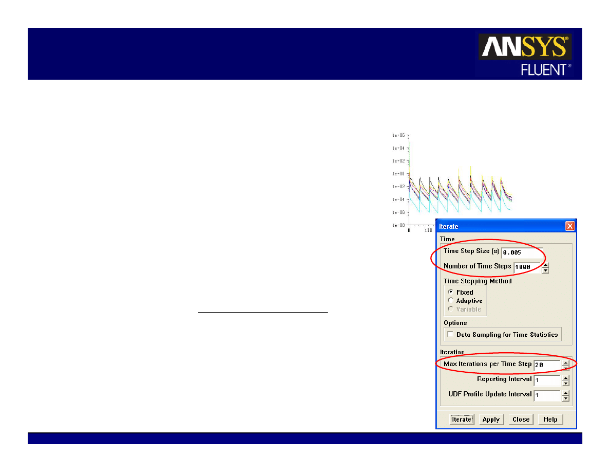
Unsteady Flow Modeling
Solver iterates to convergence within each time step, then
advances to the next.
Solution initialization defines the initial condition and it must
be realistic.
Non-iterative Time Advancement (NITA) is available for
faster computation time (see the Appendix for details).
For the pressure-based solver:
z
Time step size,
∆t, is set in the Iterate panel
∆t must be small enough to resolve time-dependent
features; make sure the convergence is reached within
the number of Max Iterations per Time Step
The order of magnitude of an appropriate time step size
can be estimated as:
Time step size estimate can also be chosen so that the
unsteady characteristics of the flow can be resolved
(e.g. flow within a known period of fluctuations)
z
To iterate without advancing in time, use zero time steps
z
The PISO scheme may aid in accelerating convergence for
many unsteady flows
velocity
flow
stic
Characteri
size
cell
Typical
≈
∆t
5-32
© 2006 ANSYS, Inc. All rights reserved.
ANSYS, Inc. Proprietary
Fluent User Services Center
www.fluentusers.com
Introductory FLUENT Notes
FLUENT v6.3 December 2006
Unsteady Flow Modeling Options
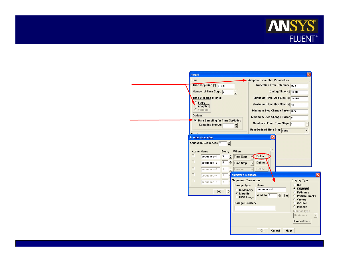
Adaptive Time Stepping
z
Automatically adjusts time-step size based
on local truncation error analysis
z
Customization possible via UDF
Time-averaged statistics
z
Particularly useful for LES turbulence
modeling
If desirable, animations should be set up
before iterating (for flow visualization)
For the density-based solver, the Courant
number defines:
z
The global time step size for density-based
explicit solver.
z
The pseudo time step size for density-
based implicit solver
Real time step size must still be defined
in the Iterate panel

5-33
© 2006 ANSYS, Inc. All rights reserved.
ANSYS, Inc. Proprietary
Fluent User Services Center
www.fluentusers.com
Introductory FLUENT Notes
FLUENT v6.3 December 2006
Summary
Solution procedure for both the pressure-based and density-based
solvers is identical.
z
Calculate until you get a converged solution
z
Obtain a second-order solution (recommended)
z
Refine the mesh and recalculate until a grid-independent solution is
obtained.
All solvers provide tools for judging and improving convergence and
ensuring stability.
All solvers provide tools for checking and improving accuracy.
Solution accuracy will depend on the appropriateness of the physical
models that you choose and the boundary conditions that you specify.

5-34
© 2006 ANSYS, Inc. All rights reserved.
ANSYS, Inc. Proprietary
Fluent User Services Center
www.fluentusers.com
Introductory FLUENT Notes
FLUENT v6.3 December 2006
Appendix
Background
z
Finite Volume Method
z
Explicit vs. Implicit
z
Segregated vs. Coupled
z
Transient Solutions
z
Flow Diagrams of NITA and ITA Schemes
5-35
© 2006 ANSYS, Inc. All rights reserved.
ANSYS, Inc. Proprietary
Fluent User Services Center
www.fluentusers.com
Introductory FLUENT Notes
FLUENT v6.3 December 2006
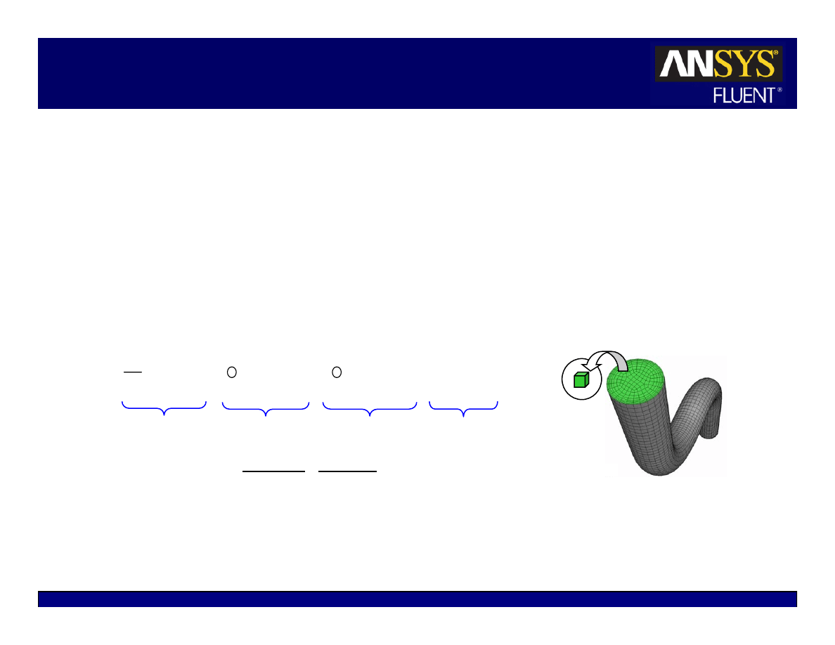
The Finite Volume Method
FLUENT
solvers are based on the finite volume method.
z
Domain is discretized into a finite set of control volumes or cells.
The general transport equation for mass, momentum, energy, etc. is
applied to each cell and discretized.
All equations are solved in order to render the flow field.
Fluid region of pipe flow
discretized into finite set of
control volumes (mesh).
control
volume
∫
∫
∫
∫
φ
+
⋅
φ
∇
Γ
=
⋅
φ
ρ
+
φ
ρ
∂
∂
V
A
A
V
dV
S
d
d
dV
t
A
A
V
Unsteady
Convection
Diffusion
Generation
Equation Variable
Continuity
1
X momentum
u
Y momentum
v
Z momentum
w
Energy
h
5-36
© 2006 ANSYS, Inc. All rights reserved.
ANSYS, Inc. Proprietary
Fluent User Services Center
www.fluentusers.com
Introductory FLUENT Notes
FLUENT v6.3 December 2006
The Finite Volume Method
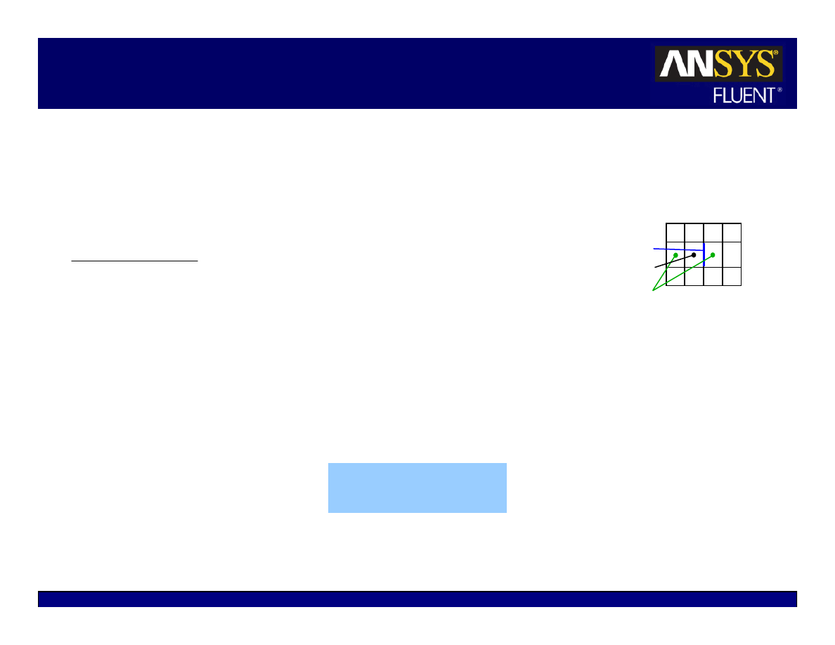
Each transport equation is discretized into algebraic form. For cell P,
Discretized equations require information at both cell centers and
faces.
z
Field data (material properties, velocities, etc.) are stored at cell centers.
z
Face values are interpolated in terms of local and adjacent cell values.
z
Discretization accuracy depends on the “stencil” size.
The discretized equation can be expressed simply as
z
Equation is written for every control volume in the domain resulting in an
equation set.
face f
adjacent cells, nb
cell p
p
nb
nb
nb
p
p
b
a
a
=
φ
+
φ
∑
( )
( )
( )
V
S
A
A
V
V
t
f
f
f
f
f
f
f
t
p
t
t
p
∆
+
φ
∇
Γ
=
φ
ρ
+
∆
∆
ρφ
−
ρφ
φ
⊥
∆
+
∑
∑
faces
,
faces

5-37
© 2006 ANSYS, Inc. All rights reserved.
ANSYS, Inc. Proprietary
Fluent User Services Center
www.fluentusers.com
Introductory FLUENT Notes
FLUENT v6.3 December 2006
Linearization
Equation sets are solved iteratively.
z
Coefficients a
p
and a
nb
are typically functions of solution
variables (nonlinear and coupled).
z
Coefficients are written to use values of solution variables
from the previous iteration.
Linearization removes the coefficients’ dependence on
φ.
Decoupling removes the coefficients’ dependence on other
solution variables.
z
Coefficients are updated with each outer iteration.
For a given inner iteration, coefficients are constant
(frozen).
φ
p
can either be solved explicitly or implicitly.
p
nb
nb
nb
p
p
b
a
a
=
φ
+
φ
∑

5-38
© 2006 ANSYS, Inc. All rights reserved.
ANSYS, Inc. Proprietary
Fluent User Services Center
www.fluentusers.com
Introductory FLUENT Notes
FLUENT v6.3 December 2006
Explicit vs. Implicit Solution
Assumptions are made about the knowledge of
φ
nb
.
z
Explicit linearization
Unknown value in each cell computed from relations that include only
existing values (
φ
nb
assumed known from previous iteration).
φ
p
is then solved explicitly using a Runge-Kutta scheme.
z
Implicit linearization
φ
p
and
φ
nb
are assumed unknown and are solved using linear equation
techniques.
Equations that are implicitly linearized tend to have less restrictive
stability requirements.
The equation set is solved simultaneously using a second iterative loop
(e.g., point Gauss-Seidel).

5-39
© 2006 ANSYS, Inc. All rights reserved.
ANSYS, Inc. Proprietary
Fluent User Services Center
www.fluentusers.com
Introductory FLUENT Notes
FLUENT v6.3 December 2006
Pressure-Based vs. Density-Based Solver
Pressure-based solver
z
If the only unknowns in a given equation are assumed to be for a single
variable, then the equation set can be solved without regard to the solution
of other variables.
z
Simply put, each governing equation is solved independently of the other
equations).
z
In this case, the coefficients a
p
and a
nb
are scalar values.
Density-based solver
z
If more than one variable is unknown in each equation, and each variable
is defined by its own transport equation, then the equation set is coupled
together.
z
In this case, the coefficients a
p
and a
nb
are N
eq
× N
eq
matrices.
z
φ is a vector of the dependent variables, {p, u, v, w, T, Y}
T
p
nb
nb
nb
p
p
b
a
a
=
φ
+
φ
∑
5-40
© 2006 ANSYS, Inc. All rights reserved.
ANSYS, Inc. Proprietary
Fluent User Services Center
www.fluentusers.com
Introductory FLUENT Notes
FLUENT v6.3 December 2006
Pressure-Based Solver
In the pressure-based solver, each
equation is solved separately.
The continuity equation takes the
form of a pressure correction equation
as part of Patankar’s SIMPLE
algorithm.
Under-relaxation factors are included
in the discretized equations.
z
Included to improve stability of
iterative process.
z
An explicit under-relaxation factor, α,
limits change in variable from one
iteration to the next:
p
p
p
φ
∆
α
+
φ
=
φ
old
,
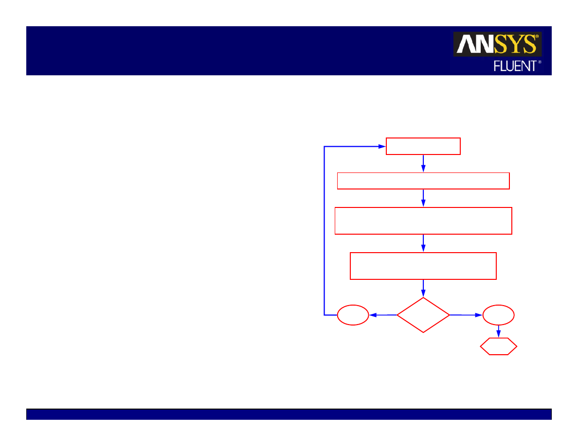
Update properties
Solve momentum equations (u, v, w velocity)
Solve pressure correction (continuity) equation
Update pressure field and face mass flow rates
Solve energy, species, turbulence, and
other scalar equations
Yes
No
Converged?
Stop
5-41
© 2006 ANSYS, Inc. All rights reserved.
ANSYS, Inc. Proprietary
Fluent User Services Center
www.fluentusers.com
Introductory FLUENT Notes
FLUENT v6.3 December 2006
Density-Based Solver
Continuity, momentum, energy, and
species are solved simultaneously in the
density-based solver.
Equations are modified to resolve both
compressible and incompressible flow.
Transient term is always included.
z
Steady-state solution is formed as time
increases and transients tend to zero.
For steady-state problem, the “time step”
is defined by the Courant number.
z
Stability issues limit the maximum time
step size for the explicit solver but not for
the implicit solver.
(
)
U
x
t
∆
=
∆
CFL
CFL = Courant-Friedrichs-Lewy-number
u = appropriate velocity scale
∆
x = grid spacing
Update properties
Solve continuity, momentum, energy
and species equations simultaneously
Solve turbulence and other scalar equations
Yes
No
Converged?
Stop
5-42
© 2006 ANSYS, Inc. All rights reserved.
ANSYS, Inc. Proprietary
Fluent User Services Center
www.fluentusers.com
Introductory FLUENT Notes
FLUENT v6.3 December 2006
Multigrid Solver
The Multigrid solver accelerates convergence by solving
the discretized equations on multiple levels of mesh
density so that the “low-frequency” errors of the
approximate solution can be efficiently eliminated
z
Influence of boundaries and far-away points are more easily
transmitted to interior of coarse mesh than on fine mesh.
z
Coarse mesh defined from original mesh
Multiple coarse mesh ‘levels’ can be created.
Algebraic Multigrid (AMG) – coarse mesh emulated
algebraically
Full Approximate Storage Multigrid (FAS) – ‘cell
coalescing’ defines new grid.
–
An option in the density-based explicit solver.
Final solution is for original mesh
z
Multigrid solver operates automatically in the background
Consult the FLUENT User’s Guide for additional options
and technical details
Fine (original) mesh
coarse mesh
“Solution
Transfer”
5-43
© 2006 ANSYS, Inc. All rights reserved.
ANSYS, Inc. Proprietary
Fluent User Services Center
www.fluentusers.com
Introductory FLUENT Notes
FLUENT v6.3 December 2006
Background: Coupled/Transient Terms
Coupled solver equations always contain a transient term.
Equations solved using the unsteady coupled solver may contain two transient terms:
z
Pseudo-time term,
∆τ.
z
Physical-time term,
∆t.
Pseudo-time term is driven to near zero at each time step and for steady flows.
Flow chart indicates which time step size inputs are required.
z
Courant number defines
∆τ
z
Inputs to Iterate panel define
∆t.
Coupled Solver
Explicit
Implicit
Steady Unsteady
Steady Unsteady
∆τ, ∆t
∆τ
∆τ, ∆t
∆τ
∆τ
⇐ pseudo-time
Explicit
Implicit
⇐ physical-time
Implicit
Discretization of:
(global time step)
5-44
© 2006 ANSYS, Inc. All rights reserved.
ANSYS, Inc. Proprietary
Fluent User Services Center
www.fluentusers.com
Introductory FLUENT Notes
FLUENT v6.3 December 2006
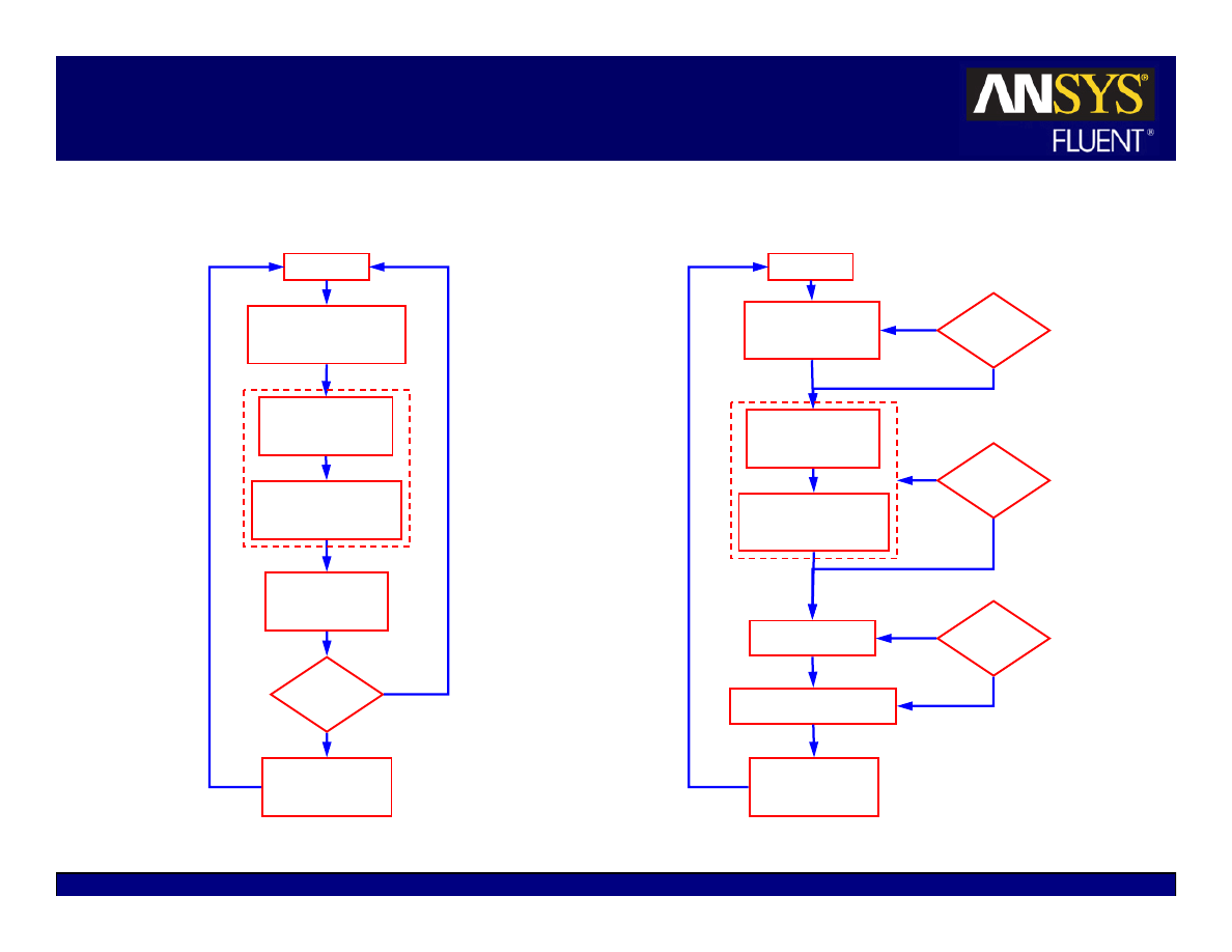
ITA versus NITA
Non-Iterative Time Advancement (NITA)
Iterative Time Advancement (ITA)
t
n
t
t
∆
+
=
Converged?
Solve U, V, W
equations
Solve k and ε
Solve other scalars
Advance to
next time step
Converged?
Converged?
Solve pressure
correction
Correct velocity,
pressure, fluxes
Yes
Yes
Yes
No
No
No
t
n
t
t
∆
+
=
Solve momentum
equations
Solve scalars
(T, k, ε, etc.)
Advance to
next time step
Converged?
Solve pressure
correction
Correct velocity,
pressure, fluxes
Yes
No
5-45
© 2006 ANSYS, Inc. All rights reserved.
ANSYS, Inc. Proprietary
Fluent User Services Center
www.fluentusers.com
Introductory FLUENT Notes
FLUENT v6.3 December 2006
NITA Schemes for the Pressure-Based Solver
Non-iterative time advancement (NITA) schemes reduce the splitting error to
O(∆t
2
) by using sub-iterations (not the more expensive outer iterations to
eliminate the splitting errors used in ITA) per time step.
NITA runs about twice as fast as the ITA scheme.
Two flavors of NITA schemes available in FLUENT 6.3:
z
PISO (NITA/PISO)
Energy and turbulence equations are still loosely coupled.
z
Fractional-step method (NITA/FSM)
About 20% cheaper than NITA/PISO on a per time-step basis.
NITA schemes have a wide range of applications for unsteady simulations,
such as incompressible, compressible (subsonic, transonic), turbomachinery
flows, etc.
NITA schemes are not available for multiphase (except VOF), reacting flows,
porous media, and fan models, etc. Consult the FLUENT User’s Guide for
additional details.
Truncation error:
O(
∆t
2
)
Splitting error (due to eqn
segregation): O(
∆t
n
)
Overall time-discretization error
for 2
nd
-order scheme:
O(
∆t
2
)
=
+
5-46
© 2006 ANSYS, Inc. All rights reserved.
ANSYS, Inc. Proprietary
Fluent User Services Center
www.fluentusers.com
Introductory FLUENT Notes
FLUENT v6.3 December 2006
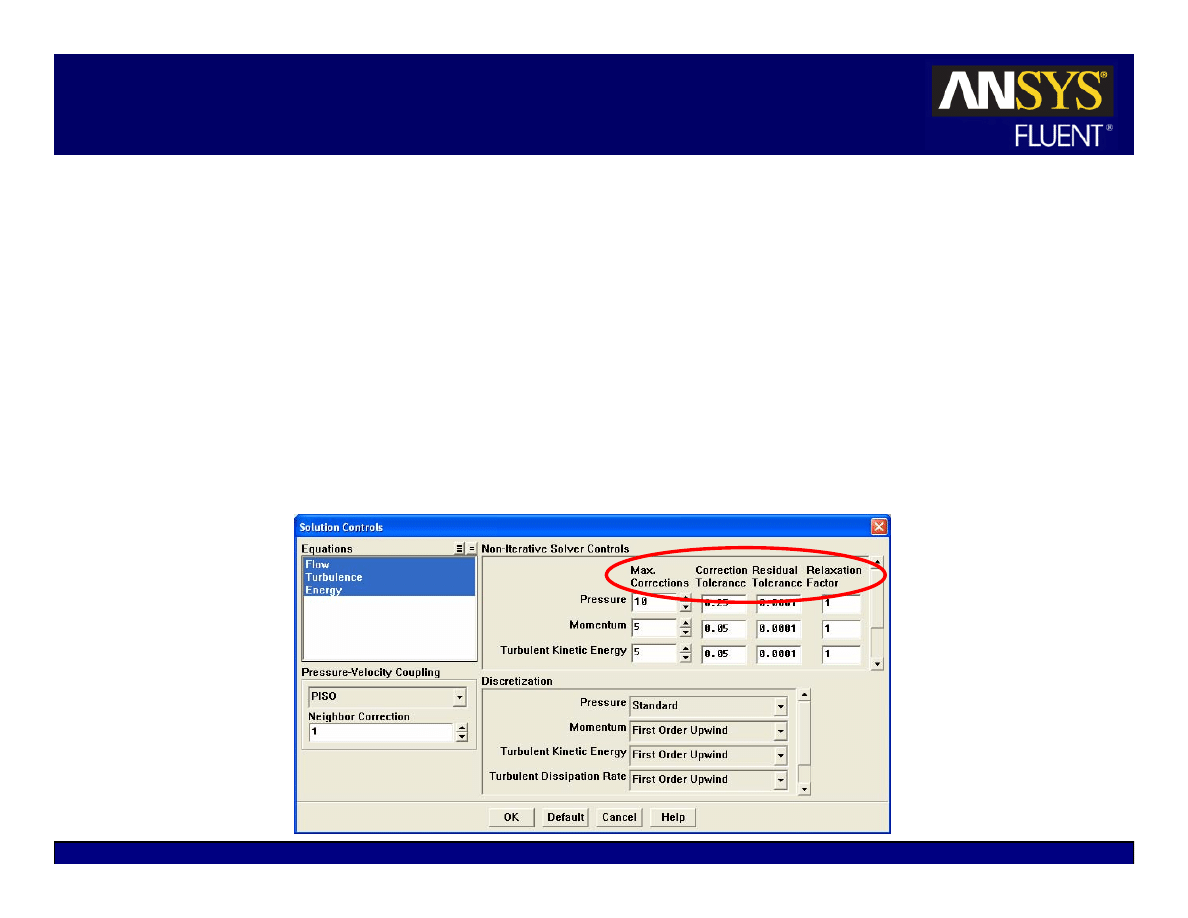
NITA Solution Control and Monitoring
Sub-iterations are performed for discretized equations till the Correction
Tolerance is met or the number of sub-iterations has reached the Max Corrections
Algebraic multigrid (AMG) cycles are performed for each sub-iteration. AMG
cycles terminate if the default AMG criterion is met or the Residual Tolerance is
sastisfied for the last sub-iteration
Relaxation Factor is used for solutions between each sub-iteration
Wyszukiwarka
Podobne podstrony:
wfhss training 1 04 pl
04 The Routledge Introductory Persian Course Supplement
17 BMW New CKM Introduction & Setting
Tatum Throne Hard Hits 04 Training Levi
Wykład 04
04 22 PAROTITE EPIDEMICA
IntroductoryWords 2 Objects English
lecture3 complexity introduction
Introduction to VHDL
04 Zabezpieczenia silnikówid 5252 ppt
Wyklad 04
Wyklad 04 2014 2015
04 WdK
04) Kod genetyczny i białka (wykład 4)
2009 04 08 POZ 06id 26791 ppt
2Ca 29 04 2015 WYCENA GARAŻU W KOSZTOWEJ
04 LOG M Informatyzacja log
więcej podobnych podstron