
Creating a Profitable Betting Strategy for Football by Using Statistical Modelling
Niko Marttinen
M.Sc., September 2001
Department of Statistics
Trinity College Dublin
Supervisor: Kris Mosurski

i
Abstract
Our goal was to investigate the possibility of creating a profitable betting strategy for
league football. We built the Poisson model for this purpose and examined its
usefulness in the betting market. We also compared the Poisson model against other
most commonly used prediction methods, such as Elo ratings and multinomial
ordered probit model. In the thesis, we characterized most of the betting types but
were mainly focused on fixed odds betting. The efficiency of using the model in
more exotic forms of betting, such as Asian handicap and spread betting, was also
briefly discussed.
According to market research studies, sports betting will have an increasing
entertainment value in the future with the penetration of new technology. When
majority of government-licensed bookmakers are making their transition from online
terminals into the Internet, the competition will increase and bring more emphasis on
risk management. In this thesis, we investigated the benefits of using a statistically
acceptable model as a support of one’s decisions both from bookmaker's and punter's
point of views and concluded that it would have potential to improve their
performance.
The model proposed here was proven to be useful for football betting purposes. The
validation indicated that it quite effectively captured many aspects of the game and
finally enabled us to finish the season with positive return.

ii
1 Introduction ................................................................................................. 1
1.1
Structure of League Football ................................................................ 2
1.2
Betting on Football............................................................................... 3
1.2.1 Pari-mutuel
Betting ...................................................................... 3
1.2.2
Fixed Odds Betting....................................................................... 4
1.2.3
Asian Handicap (Hang Cheng) ..................................................... 5
1.2.4
Asian Handicap vs. Fixed Odds .................................................... 8
1.2.5 Spread
Betting.............................................................................. 9
1.2.6 Person-to-person
Betting ............................................................ 10
1.3 Betting
Issues..................................................................................... 11
1.4 Return
Percentage .............................................................................. 12
1.5 Internet
Betting .................................................................................. 13
1.6 Taxation............................................................................................. 18
1.7
Scope of the Thesis ............................................................................ 19
2 Literature
Review ...................................................................................... 21
2.1 Maher-Poisson
Approach ................................................................... 21
2.2
Alternative Prediction Schemes.......................................................... 26
2.2.1
Elo Ratings and Bradley-Terry Model ........................................ 27
2.2.2
Multinomial Ordered Probit Model............................................. 30
2.3 Betting
Strategies ............................................................................... 31
2.3.1
Unconstrained Optimal Betting for Single Biased Coin .............. 32
2.3.2
Unconstrained Optimal Betting for Multiple Biased Coins.......... 34
2.3.3
More on Kelly Criterion ............................................................. 35
3
Data Description and Model Formulation................................................... 37
3.1 Data
Description ................................................................................ 37
3.2 Poisson
Regression
Formulation......................................................... 38
3.2.1 Assumptions............................................................................... 38
3.2.2 Basic
Model ............................................................................... 41
3.2.3
Separate Home Parameter Model................................................ 47
3.2.4
Split Season Model..................................................................... 50
3.2.5
Comparison among Poisson Models with Full Season Data ........ 50
3.2.6
Odds Data and E(Score) Model .................................................. 51
3.2.7
Poisson Correction Model .......................................................... 53
3.2.8 Weighted
Model......................................................................... 55
3.3
Comparison among Poisson Models Week-by-week .......................... 58
3.4 Elo
Ratings ........................................................................................ 60
3.5
Multinomial Ordered Probit Model .................................................... 62
3.6
Comparison of Approaches ................................................................ 64
4
Betting Strategy and Model Validation ...................................................... 65
4.1 Value
Betting ..................................................................................... 65
4.2 Betting
Strategy ................................................................................. 66
4.3 Money
Management........................................................................... 66
4.4
Validation on Existing Data ............................................................... 67
5 Discussion ................................................................................................. 71
5.1
Implementation of the System ............................................................ 71
5.2
Applications of the System................................................................. 72

iii
5.2.1
Bookmaker’s Point of View........................................................ 73
5.2.2
Punter’s Point of View ............................................................... 73
6
Summary and Future Work ........................................................................ 75
6.1 Summary............................................................................................ 75
6.2 Future
Work....................................................................................... 75
6.2.1 Residual
Correction .................................................................... 76
6.2.2
Other Types of Betting ............................................................... 76
6.2.3 Bayesian
Framework .................................................................. 79
Appendices........................................................................................................ 80
Appendix A ................................................................................................... 80
Appendix B ................................................................................................... 81
Appendix C ................................................................................................... 82
Appendix D ................................................................................................... 83
References......................................................................................................... 88

1
Chapter 1
1 Introduction
Independent forecasters predict an explosive growth in global online betting.
Ernst & Young (2000) claim in their market research paper that the driving force
of Internet and digital technology will open up mass-market sports betting by
delivering live entertainment, news and information to Internet linked PC’s,
mobile phones and interactive television. More and more people have access to
the Internet, which has evolved the sports betting business among other e-
commerce businesses. It is inevitable that this change will bring new forms of
betting into the picture. For example, so far the only live action betting has been
spread betting. The spread betting firms accept the bets made “in running”, which
means that the bets can also be placed while the event is going on. If the player
notices that one has few bets going against him/her, those bets can be sold in
order to minimize the losses. The only reason why spread betting has not fully
taken off is its complexity. In order to attract casual punters, the game format
needs to be quite simple. Balancing between simplicity and people’s interest
requires a lot of creativity. Recently introduced person-to-person betting has
effectively captured both these criteria. Punters can take each other on in several
different topics and the gaming operator monitors and settles all the bets.
Whether it is fixed odds, tote, spread or person-to-person betting, wagering will
be much faster in the future and the requirements for the system operating this
increase accordingly.
Security, speed and pricing are the most crucial issues that will distinguish the
profitable Internet sports books from the failing ones. Technology providers are
responsible for the first two, but odds compilers mostly cover the pricing issues.

2
Currently, the odds compilers work in teams of three or four experts, with one
head odds compiler making the final decision about what prices to release to
punters. The alternative is to buy the odds from a consultant. Usually, odds
compilers use several ad hoc techniques and their expert opinion in compiling
final prices. In order to manage risks while competing with better prices in the
market, a proper statistical tool should be developed for gaming operators. The
purpose of this thesis is to create a model that is capable of predicting results of
football matches with reasonable accuracy and to compare it to other forecasting
techniques and the odds collected from a bookmaker. We investigate whether it is
possible to create a profitable betting strategy by using statistical modelling. The
pricing issues are thus examined both from the punter’s and the bookmaker’s
point of views.
In order to create a profitable betting strategy, one must be capable of estimating
the probability of each outcome accurately enough. How accurately, depends on
the level of the opposition. The opposition could be either a bookmaker or other
punters. The goal of our study has been to establish a proper method for this
estimation. The focus is in the football betting market. In this chapter, we first
take a brief look at the structure of league football and the betting market.
1.1 Structure of League Football
The reason for our focus on league football is because of its simplicity and data
availability. Cup matches and international tournaments create problems due to
the variability of participants and lack of consistent data. The most common
format in the league football is a double round robin tournament, where each team
plays against each other twice, once at home and once away. This way it is
possible to eliminate the bias of a home advantage. Most of the major leagues in
Europe are played in this format. Different variations are used in some countries,
such as round robin and playoff combination or single/triple round robin, but we

3
restrict our attention solely to double round robin tournament because of its
simplicity and popularity. A match outcome, in a round robin tournament, is
converted to points that reflect the value attached to each outcome (3 points for a
win, 1 for a draw and 0 for a loss). These points accumulate during a season and
the team with the highest number of points wins the league.
The teams’ ability changes over the course of a season due to things such as
injuries, transfers, suspensions, motivation, etc. Therefore, determining the
probabilities for each outcome in a particular match is not that straightforward.
Lots of things need to be taken into consideration before the final conclusions can
be made. Many of these things are hard to quantify and difficult to use in a
numerical analysis.
1.2 Betting on Football
Football is the most popular sport in the world, and also the most popular sport in
betting. The most traditional bet is to place money on the outcome of a match.
Whether the match will end to a home win, a draw, or an away win. Also, correct
score, halftime/fulltime, handicap, total goals and future outright bets (f. ex.
betting on the winner of the championship) are popular. In addition, there are
nowadays numerous exotic variations of football betting, especially in spread
betting where punters can bet on bookings, shirt numbers, corner kicks, etc.
during a match. We take a look at the different types of betting in the following
sections.
1.2.1 Pari-mutuel Betting
In pari-mutuel betting the bookmakers take their money off the top, and the rest is
distributed equally among the winners. A punter is competing against other
punters in this type of betting. The more familiar name for this betting type is the

4
Tote. The odds are purely a function of betting volume’s reaction, so the
bookmaker is playing safe in pari-mutuel betting. This is very common in horse
racing, but also football pools work in this way. Out of certain number of
matches the punter is required to pick one or more choices for each match. Very
often, the home win is denoted as 1, the draw as X, and the away win as 2, and
hence football pool is synonymous to 1X2-betting. On the coupon of twelve
matches, the punter usually needs to predict ten or more outcomes correctly in
order to receive any payoff. This is probably the most traditional football betting
type. For a professional punter, though, it is not as exciting as other types listed
below, because of the low return percentage. Some of the correct score and future
outright bets are also based on pari-mutuel structure.
1.2.2 Fixed Odds Betting
Fixed odds betting has increased its popularity very rapidly. There are more
chances for profitable betting because the return percentage is greater than in
football pools (sometimes even as high as 95 %). The bookmaker offers odds for
each possible outcome in a match and the punter will determine which ones are
worth betting on. For example, in a match Liverpool against Chelsea the
bookmaker offers the following odds:
Home team
Away team
Odds home
Odds draw
Odds away
Liverpool
Chelsea
2.00
2.60
3.00
If the punter has chosen to back Liverpool with £10 and Liverpool wins the
match, the punter will get his/her stake multiplied by the odds for Liverpool’s
victory. In this case the punter’s gross win would be £20 and the net win £10. If
on the other hand the match had ended to a draw or Chelsea’s victory, the punter
would have lost his/her stake.

5
In Great Britain and Ireland, the odds are the form x/y (say 1/2, where you need to
bet 2 units to win 1 unit). On mainland Europe, the more common way to present
odds is the inverse of a probability, called a dividend as in the example above.
The traditional odds are converted to dividend odds by dividing x by y and adding
one. Thus, 1/2 means 1.50 in European scale. The table of conversions is
presented in Appendix A.
Some bookmakers do not accept bets on a single match. Instead a punter needs to
pick two, three or more matches on the same coupon. The matches are
independent events, so this way the bookmaker decreases the return percentage to
the punters. For example, if the bookmaker returns 80 % of the total money
wagered and requires punters to pick at least three matches, the theoretical return
percentage diminishes to 0.8
3
= 51.2 %. Fortunately from the punter’s point of
view, increasing competition in the betting market forces bookmakers to offer
better odds and ability to bet on single events or they go out of business. We take
a closer look at the return percentage later on in this chapter.
In fixed odds betting, the odds are generally published a few days before the
event. Internet bookmakers can change their odds many times before the match
takes place responding to the betting volume’s reactions. Their job is to keep the
money flow in balance and thus guarantee the “fixed” revenue for the gaming
operator. For the traditional High Street bookmaker altering odds on a coupon
requires enormous reprinting efforts, whereas for the Internet bookmaker it
happens just by clicking a mouse. Other popular fixed odds bets are correct score,
first goal scorer, halftime/fulltime and future outright bets.
1.2.3 Asian Handicap (Hang Cheng)
In Far East, handicap betting is more popular than traditional fixed odds betting.
The approach, derived from the Las Vegas sports books, has expanded its

6
popularity to Europe as well. In Asian handicap, the bookmaker determines a
predicted superiority (a difference between home goals and away goals). One
team gets, let’s say, 1/2 goal ahead before the start of a match. Thus the draw is
normally eliminated in Asian handicap and the odds are set for two outcomes.
The fundamental idea is to create even odds in a match by means of a handicap.
With Asian Handicap, there is a much better chance of profit, due to the fact that a
punter may get his/her stake back (or at least parts of it, depending on the
handicap). In fixed odds betting, one would lose money if wagered on something
else than the correct outcome. You can bet on teams which you really do not
believe will win the match, but due to the handicap, your team may still provide
you a value opportunity. Asian Handicap betting also provides much more
excitement, as one single goal in a match counts much more than in fixed odds
betting. The worst thing in Asian Handicap, in our opinion, is a rather complex
way of figuring out the return. You will also need an account with companies
offering Asian Handicap, as not all bookmakers offer it.
Below, we offer few examples of Asian handicap bets.
Example 1:
Milan-Juventus
The handicap is:
Home team
Away team Odds home Handicap Odds away
Milan
Juventus
2.00
0 : ½
1.85
Bet on Milan:
•
If Milan wins the match you will win stake x 2.00, otherwise you will lose
Bet on Juventus:
•
If the match ends in a draw or Juventus wins you will win stake x 1.85

7
Example 2:
Arsenal-Leeds
The handicap is:
Home team
Away team Odds home Handicap Odds away
Arsenal
Leeds
1.925
0 : ½
1.975
Bet on Arsenal:
•
If Arsenal wins the match by two goals or more you will win stake x 1.925
•
If Arsenal wins the match by one goal you will win: 1.925 x 0.5 x stake +
stake
Bet on Leeds:
•
If the match ends in a draw or Leeds wins you will win stake x 1.975
•
If Arsenal wins the match by one goal you will win stake x 0.5
Example 3:
Barcelona-Real Madrid
The handicap is:
Home team
Away team Odds home Handicap Odds away
Barcelona Real Madrid 1.925
0 : 1
1.975
Bet on Barcelona:
•
If Barcelona wins the match by two goals or more you will win stake x
1.925
•
If Barcelona wins the match by one goal you will get your stake back
Bet on Real Madrid:

8
•
If the match ends in a draw or Real Madrid wins you will win stake x
1.975
•
If Barcelona wins the match by one goal you will get your stake back
1.2.4 Asian Handicap vs. Fixed Odds
The advantages of two different ways to bet on a football match:
Asian Handicap
•
Normally eliminates the possibility of a draw
•
If a quarter handicap match ends in a draw, you only lose 50% of your
stake
•
Entertaining when following a match live - one single goal is likely to
change everything
•
When playing multiple matches, the number of outcomes compared to
1X2-betting is reduced from 27 (3x3x3) to only 8 (2x2x2)
Fixed Odds
•
A very wide range of bookmakers to choose from
•
It is possible to bet on "secure" matches, which might be suitable for
accumulator bets
•
Much easier to find value bets. You only need home-draw-away
estimations, in Asian Handicap it is required that you are able to predict
goals scored

9
1.2.5 Spread Betting
Harvey (1998) and Burke (1998) both conclude in their books that in spread
betting there is a great volatility, which provides excitement but exposes the
punter to risks of substantial losses, as well as rewards. It is one of the fastest
growing areas of gaming. It all started in early 1980’s when two founder
members of City Index began betting on the winning race card numbers at the
Arch de Triumph race meeting when they could not make a bet because the
queues were too long at the French Tote betting windows. The fundamental idea
is that the more you are right the more you win, and vice versa.
You can bet money on a variety of events such as the number of corner kicks,
bookings, total goals, etc. The way the spread betting works is that the spread
betting company determines the spread for a certain event. For example, in
Arsenal-Manchester United match at Highbury the spread betting agency has
determined the spread for total goals as 2.1-2.4. The punter can either buy this
commodity from them at 2.4 or sell to them at 2.1. Let the final score be 1-1. If a
punter had sold the commodity at 2.1 with the stake of £10 per tenth of a goal, he
would have made a £10 profit. If on the other hand, he had bought that at 2.4
with the same stake, he would have lost £40. It is important to grasp the concept
that you always buy at the top of the spread and sell at the bottom of the spread.
There are many similarities between stock market and spread betting. Most of the
spread betting companies primary interest is actually the financial spread betting.
The punter’s aim is to predict the movement, for example, in the FTSE
TM
100
index in a similar way. Financial spread betting is a tax-free alternative to
traditional trading in stock market. It covers variety of currency, commodity and
bond futures markets. An interesting aspect in spread betting is that you can place
a bet “in running”, which means that while the event is going on, you can get rid
off your losing bets or buy more profitable ones. One major setback in spread
betting is rather big deposit and the complex registration procedure, which are

10
required by spread betting companies due to the fact that they are governed by the
Financial Services Act (FSA). Therefore it is not meant for casual punters. It can
be very risky as losses are potentially unlimited. It needs a thorough
understanding of the system, before one should start betting. The biggest
companies offering spread betting are City Index, IG Index, and Sporting Index.
1.2.6 Person-to-person Betting
It is surprising, how new thing person-to-person betting is considering its
simplicity. For the operator, it is completely risk free. Therefore, we believe that
it will become popular among sports books as a subsidiary form of betting. The
idea of person-to-person betting is characterized below:
•
Punters set their own odds and others can decide whether or not to take
them on. The website acts like a clearing house, monitoring and settling
all the bets
•
Two punters are thus involved in one bet
•
Not betting against faceless corporation but other punters
•
More realistic and adventurous odds than offered by the bookmaker
•
Concept incorporates some of the elements of spread betting in that
punters can be very specific with their bets
•
The companies make money by taking 5% from each bet, 2.5% from each
punter compared to regular betting offices who normally charge 6.75% tax
plus commission
•
Aim is to attract casual punters, not hardcore gamblers. Normally bets are
around £5-£15
•
Expected to be popular among sports fans and members of financial
institutions as a good speculation forum
•
It is estimated that more than £55 billion changed hands in the unofficial
person-to-person betting market worldwide in 1999

11
1.3 Betting Issues
Sports betting is an area of gaming in which the player is not in direct competition
with the house. In most of casino games (such as craps, keno, slot machines,
baccarat, black jack and roulette), the house has a statistical advantage. In sports
betting, however, players can gain an advantage on the house when they can
identify the events where the offered odds do not accurately reflect the true odds
for the events’ outcome. The punter needs to realize that the offered odds are not
an odds compiler’s prediction of event’s outcome. Rather, the odds are designed
so that equal money would be bet among all outcomes.
Bookmakers make their money at the expense of the people who bet impulsively.
For most punters, the main thing about betting is to add little extra excitement to
the sporting event. Therefore, it is vital for a bookmaker to create odds such that
the distribution of betting volume is in balance. Probably the most famous among
the current handicappers in Las Vegas, Michael “Roxy” Roxborough, has been
quoted: “I am not in the business to predict the outcomes, I am in the business to
divide the public opinion about these outcomes” (1999). If the betting volume is
evenly distributed, the bookmakers will always get their in-built percentage.
Thus, the odds are not always the appropriate measures of the teams’ relative
strengths. If a punter is capable of predicting the outcome correctly, there are
chances for profitable betting. The main rule for the punter is to be selective.
Only bet if the odds are on your side. If Brazil is expected to beat Poland 19
times out of 20, then the odds 1/9 (which says that Brazil wins 18 times out of 20)
are a good value. This strategy is called value betting. The punter needs to look
for the best values from the coupon and decide how much he/she is willing to
invest in them. We will take a closer look at value betting in Chapter 4.

12
1.4 Return Percentage
The website best-bets.com has a concept called QI. Standing for “Quoten
Intelliqenz” in German, translated “odds intelligence”. The similarity to the IQ –
the intelligence quotient- is deliberate. The QI tells the punter how smart one has
to be in order to beat the bookmaker.
)
(
1
)
(
1
)
(
1
Awaywin
Odds
Draw
Odds
Homewin
Odds
QI
+
+
=
Eq. 1.1
In words, QI is the sum of the reciprocal values of all odds attributable to the
outcomes of an event. The QI for the match Liverpool against Chelsea with odds
2.00/2.60/3.00 is
21796
.
1
00
.
3
1
60
.
2
1
00
.
2
1
=
+
+
=
QI
The bookmaker’s take is 22 %, thus any client of this particular bookmaker has to
know at least 22% more about the possible outcomes of this match than the
bookmaker himself, otherwise the punter will not be able to break even in the
long run.
QI
ENTAGE
RETURNPERC
1
=
Eq. 1.2
The theoretical return percentage of our soccer match is 0.82, meaning you can
expect to get 82 pence on every pound you bet on a match with this odds structure
if the bookmaker is able to receive the bets in the right proportions. The same
result is achieved when betting on each possible outcome in the match.

13
The best-bets.com concludes that QI is the most important key figure in betting
business, the lower it is, the fairer the bet. As a single bookmaker calculates the
odds in order to make a profit, the QI for the bets will be always be above 1.
On the Internet there are a number of sites (oddscomparison.com, zazewe.com,
crastinum.com and betbrain.com), which collect odds from several bookmakers.
The punter can pick the best offers among them. The competition among
bookmakers is severe, so there are often opportunities for profitable bets.
Sometimes there are even so called arbitrage opportunities, where the punter will
get a guaranteed profit by betting on all possible outcomes. The punter needs to
select the right bookmakers and to determine the stakes in an appropriate way in
order to maximize the profit when these sorts of situations occur.
1.5 Internet
Betting
Internet betting has gained a lot of popularity. The main companies such as
Ladbrokes, William Hill and Coral-Eurobet, have web sites, as do new entrants to
the market like Blue Square, Sports Internet Group and Sporting bet. The sites
usually offer links to offshore tax-free betting and provide the opportunity to bet
on most major sporting events, as well as horses and dogs. However, they do not
really provide anything more than an online alternative to telephone betting and
High Street bookmaker. Most of them have limited entertainment value and are
primarily information driven, but as customer expectations grow this will
probably change.
Despite its current popularity, Internet betting still has a huge future ahead. With
the development of new distribution channels, like digital television and mobile
phones, it will become even easier and more exciting.

14
Only thing holding back Internet betting are the legal issues. The US has recently
rejected the Kyl Bill that would have largely prohibited online gaming throughout
United States, making it a federal crime for US citizens. Many individual states,
including Nevada and New York have already chosen to take a hard line on online
gaming. This approach has led to the development of online gaming offshore,
mainly in the Caribbean, which has now become a major center directing
operations at North America. Even so, offshore relocation has not stopped some
US authorities challenging the new operations.
Until recently the Australian government tried to regulate online gaming by
allowing individual states to grant licenses to operators. However, they have now
announced a moratorium on the granting of licenses and the eventual outcome of
their review is far from clear.
In the UK it is legal to place and receive bets over the telephone or via the
Internet. However, advertising offshore gaming – telephone or Internet – is
illegal. According to Ernst & Young survey, several UK bookmakers circumvent
this contradiction by including a link (not an advert) in their websites to offshore
operations – a .co.uk site links through to a .com site. The sites look similar but
they are registered in different locations.
On mainland Europe there is very little legislation and few restrictions on gaming
or betting over the Internet. Certain countries in Asia (Singapore for example)
ban online gaming, but most legislation is aimed at prohibiting any direct
advertising and restricting the supply of gaming licenses.
Another concern with Internet betting at the moment is the security. The punter
needs to do the research in order to find out which bookmakers run the creditable
business and who is trustworthy. Otherwise the punter might face the problem
not getting his/her money back. Ernst & Young research shows that the main
inhibitor for potential customers spending on the Internet is the fear of credit or

15
debit card fraud. There are already over 650 Internet betting and gaming sites,
and the number is still growing. So while the barriers to entry for Internet betting
and gaming businesses are low, simply setting up a site is no guarantee of success.
Businesses must put customer trust high on their agenda, because purely
electronic transactions completely redefine the relationship between punters and
bookmakers.
This is especially important for online betting where the average stake is higher
than in High Street bookmakers and where the bookmaker holds a customer’s
credit card details or customer has to pay up-front into an account. On William
Hill’s site for example, they refer to themselves as “The most respected name in
British bookmaking”. Fair odds and timely payout will influence repeat business
and customer loyalty to a favored site.
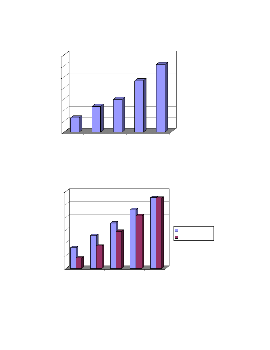
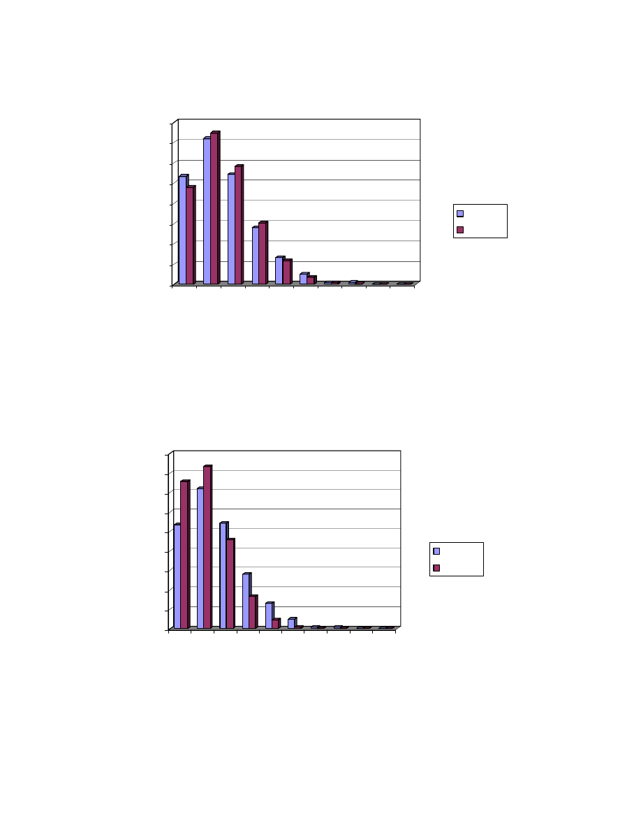
The Figure 1.1 characterizes the rapid growth of the market. In the year 2002,
according to the survey made by the River City Group (2000), estimated Internet
gaming expenditure will exceed 3 billion USD. The other survey made by
Datamonitor (1999) forecasts similar results.
16
0
500
1000
1500
2000
2500
3000
3500
1998
1999
2000
2001
2002
Estimated Worlwide Internet Gaming Expenditure (M$)
Figure 1.1 Estimated worldwide Internet gaming expenditure (Milj$). Source: River City Group
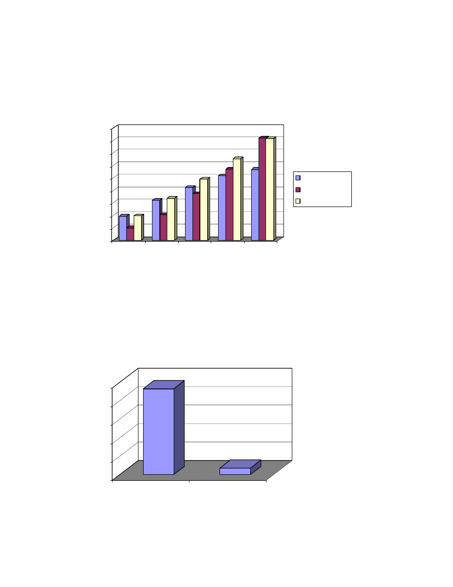
Figure 1.2 The online gaming market divided into regions (Milj. $). Source: Datamonitor
0
1000
2000
3000
4000
5000
6000
2000
2001
2002
2003
2004
USA
Western Europe
17
From Figure 1.2 it is predicted that Europe will reach America by the year 2004 in
the popularity of online gaming. Datamonitor emphasizes in their research report
that “by 2004, online games and gaming revenues will reach $16bn.”
0
500
1000
1500
2000
2500
3000
3500
4000
4500
2000
2001
2002
2003
2004
Casinos
Lotteries
Sports/events
Figure 1.3 The online gaming market divided into products (Milj. $). Source: Datamonitor
Figure 1.3 presents the product comparison among casinos, lotteries and
sports/event betting. It is predicted that lotteries and sports books are gaining
customers at faster rate compared to casinos.
0
20
40
60
80
100
Men
Women
Figure 1.4 Number of customers by sex. Source: Svenska Spel
18
Traditionally men are more eager to gaming than women are. Figure 1.4
describes that it follows the same pattern in online gaming as well. Especially,
sports betting has been male dominant, but event betting has gained a lot of
female attention according to Paddy Power, the Irish bookmaker.
0
5
10
15
20
25
30
35
40
15-24
25-34
35-44
45-54
55-64
65+
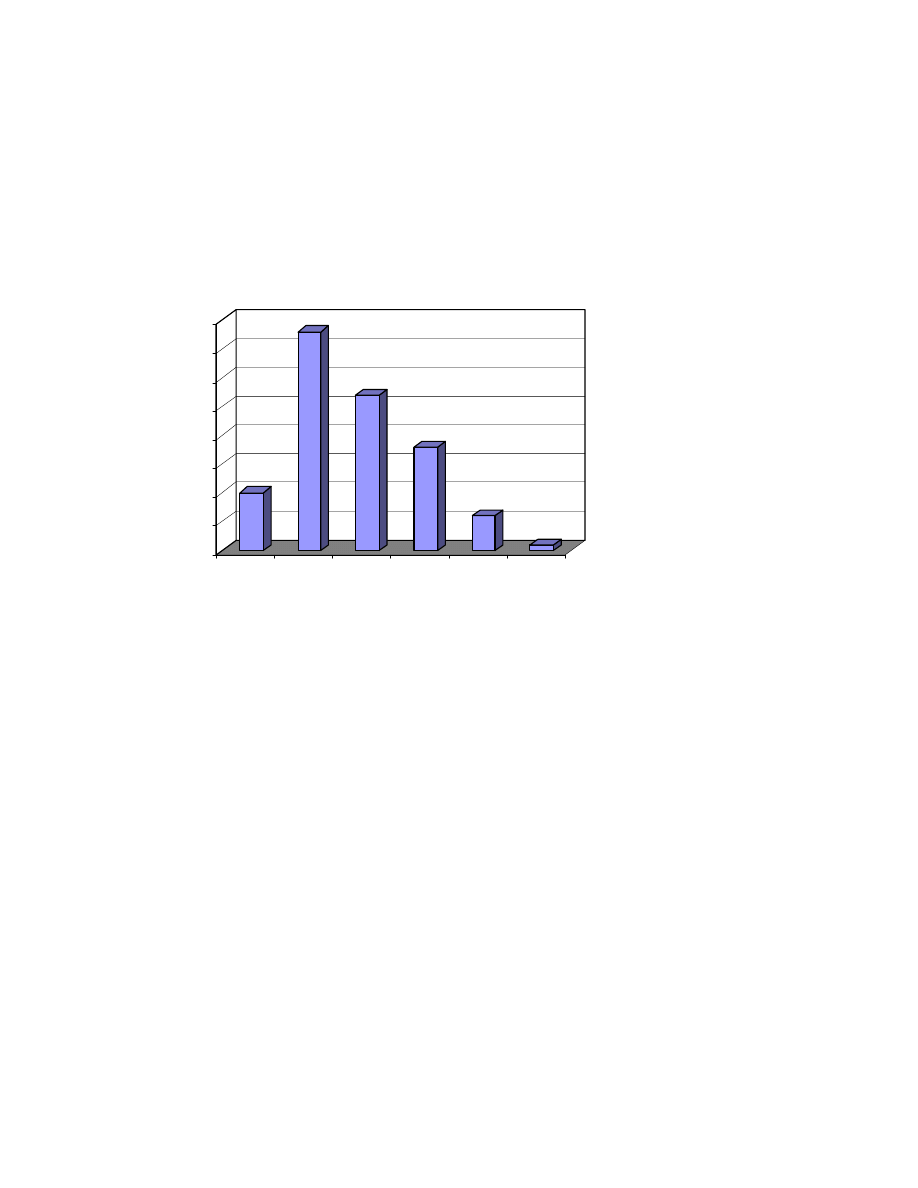
Figure 1.5
The number of customers by age. Source: Svenska Spel
Age distribution in Figure 1.5 does not provide any surprising results of the
market. The target group is the people between 25-54 years of age.
1.6 Taxation
For existing bookmakers or new entrants going online, ongoing legal situation
raises the question of where to locate their business as mentioned in Section 1.5.
Sites currently operating under British jurisdiction, for example in Gibraltar, are
held in high regard internationally because they operate to UK regulatory
standards. Good regulation and the careful granting of licenses breeds confidence
for both operators and their customers.

19
The best onshore gaming and bookmaking businesses already welcome
regulation. They recognize that it benefits their business, it reassures customers
and it provides the necessary controls to run a clean operation.
Onshore betting in the UK attracts a 9% tax whilst offshore there is 3%
administration cost. Duty in Ireland was reduced from 10% to 5% in 1998
making it a more attractive location for bookmakers. Inevitably, mainstream
bookmakers have followed Victor Chandler and set up offshore operations. All of
which favours the punter and offshore bookmaker but not the government.
The most governments are faced with a decision. If they want a slice of the
global gaming market, they will have to reduce onshore tax levels. It might even
increase their total tax-take by having a lower tax rate for a much larger market.
If they do not reduce tax, bookmakers will set up their international online
businesses in a more favourable tax climate. Even the Tote, which still is
government owned, has set up an offshore branch of its Total-bet.com site in
Malta.
1.7 Scope of the Thesis
Our goal is to study the possibility of creating a profitable betting strategy for
league football. Our main focus is in the English Premier League. In order to do
this, we need to predict the outcomes with reasonable accuracy. We build the
appropriate model for this purpose and examine its usage in the betting market.
We also compare the model against other most commonly used prediction
methods. We mainly consider the benefits of using the model in fixed odds
betting. Also, its efficiency in more exotic handicap and spread betting is
discussed in Chapter 6. Chapter 2 covers the literature relating to the subject so
far. Chapter 3 explains the model and makes comparisons against other most
common prediction methods. The betting strategy and the model validation is the

20
basis of Chapter 4. Chapter 5 covers the implementation of the system and
discusses the benefits of using it from both punter’s and bookmaker’s point of
views. In Chapter 6 we summarize the research and make a few suggestions for
future work.

21
Chapter 2
2 Literature
Review
An individual football match is a random process, where all the outcomes are
possible. Reep and Benjamin (1968) came to the conclusion that “chance does
dominate the game”. Even stronger opinion came from Hennessy (1969) who
stated that only chance was involved. Hill (1973) argued that anyone who had
ever watched a football match could reach the conclusion that the game was either
all skill or all chance. He justified his opinion by calculating the correlation
between the expert opinions and the final league tables, finding that even though
chance was involved, there was also a significant amount of talent affecting to the
final outcome of the match.
Modelling football results has not gained too much attention in a scientific
community. Most of the models punters and operators tend to use are very ad
hoc. They are not statistically justified, even though these might be useful in
betting. Most of the literature, up to date, is divided into two different schools,
either modelling the results/scores directly or observing the estimated strength
differences between teams.
2.1 Maher-Poisson Approach
Statistically, a football match can be seen as a random event, where three
outcomes are possible: a home win, a draw, and an away win. Each of them has
their own probability and the probabilities sum up to 1. Our task is to determine
these probabilities as accurately as possible. The focus is in modelling the scores,
because we believe that the scores contain more information of the teams’

22
abilities than do pure outcomes (win, draw or loss). This sort of approach is
called the Maher-Poisson approach, due to the first paper published by Maher
(1982), where he assumed that the number of goals scored by team A and team B
in a particular match had independent Poisson distributions with means,
λ
A
and
λ
B.
His article has been the basis of few others. Lee (1997) studied whether
Manchester United deserved to win the league title in 1995/1996 season. He used
Maher’s simplified model to derive the probabilities for each match and simulated
the season 1,000 times. Then he calculated the points awarded for each team and
determined the proportions of times each team topped the table. Another
important article written by Dixon and Coles (1997) investigated the
inefficiencies in the UK betting market. They used Maher’s model with few
adjustments in order to get the better fit. Dixon and Coles emphasized in their
article that in order to create a profitable betting strategy, one must consider
several aspects of the game. For example:
•
The model should take into account different abilities of both teams in a
match
•
History has proved that the team which plays at home has a home
advantage that needs to be included to our model
•
The estimate of the team’s current form is most likely to be related to its
performance in the most recent matches
•
In all simplicity, football as a game is about scoring goals and conceding
goals. Therefore, we use the separate measures of teams’ abilities to attack
and to defend
•
In summarizing a team’s performance by recent results, account should be
taken of the ability of the teams they have played against
It is not practical to estimate these aspects separately. Instead, we need to find the
statistical way to incorporate these features. In Maher’s model, he suggested that
the team i, playing at home against team j, in which the score is (x
ij
, y
ij
), and X
ij

23
and Y
ij
are independent Poisson random variables with means
αβ
and
δγ
respectively. The parameters represent the strength of the home team’s attack
(
α
), the weakness of the away team’s defence (
β
), the strength of the away team’s
attack (
δ
), and the weakness of the home team’s defence (
γ
). He finds that a
reduced model with
δ
i
= k
α
i
,
γ
i
= k
β
i
for all i is the most appropriate of several
models he investigates. Thus, the quality of a team’s attack and a team’s defence
depends on whether it is playing at home or away. Home ground advantage (1/k)
applies with equal effect to all teams.
English Premier league consists of 20 teams. The three lowest placed teams will
be relegated to Division 1 and three top teams will be promoted to the league
from Division 1 after each season. Dixon and Coles applied Maher’s model in
their article where they used all four divisions in the model. They also included
cup matches in the analysis and thus obtained a measurement for the difference in
relative strengths between divisions. We ignore cup matches in our study. Dixon
and Coles had 185 identifiable parameters, because of the number of divisions
they dealt with. In our basic model, we use only 41 parameters. Attack and
defence parameter for each team, and a common home advantage parameter. We
set Arsenal’s attack parameter to zero as our base parameter.
For clarity, we use slightly different notation than in Maher’s paper. We assume
that the number of goals scored by the home team has a Poisson distribution with
mean
λ
HOME
and the number of goals scored by the away team has a Poisson
distribution
λ
AWAY
. One match is seen as a bivariate Poisson random variable
where the goals are events, which occur during this 90-minute time interval. The
mean
λ
HOME
reflects to the quality of the home attack, the quality of the away
defence, and the home advantage. The mean
λ
AWAY
reflects the quality of the
away attack, and the quality of the home defence. These are specific to each
team’s past performance. The mean of the Poisson distribution has to be positive,
so we say that the logarithm of the mean is a linear combination of its factors.

24
Log (
λ
HOME
)
=
β
HOME
*z
1
+
β
HOMEATTACK
*z
2
+
β
AWAYDEFENCE
*z
3
Log (
λ
AWAY
) =
β
AWAYATTACK
*z
4
+
β
HOMEDEFENCE
*z
5
Eq. 2.1
Log (E(Y)) =
β
HOME
*z
1
+
β
HOMEATTACK
*z
2
+
β
AWAYDEFENCE
*z
3
+
β
AWAYATTACK
*z
4
+
β
HOMEDEFENCE
*z
5
Eq. 2.2
where
z
1
= 1 if Y refers to goals scored by home team
= 0 if Y refers to goals scored by away team;
z
2
= 1 if Y refers to goals scored by home team
= 0 if Y refers to goals scored by away team;
z
3
= 1 if Y refers to goals scored by home team
= 0 if Y refers to goals scored by away team;
z
4
= 0 if Y refers to goals scored by home team
= 1 if Y refers to goals scored by away team;
z
5
= 0 if Y refers to goals scored by home team
= 1 if Y refers to goals scored by away team.
This is a simplified equation because in reality there would be team specific
attack and defence parameters, so in the English Premier League where 20 teams
are competing the amount of z
i
’s would be 41. This is an example of a log-linear
model, which is the special case of the generalized linear models. The theory of
generalized linear models was obtained from the books by McCullach and Nelder
(1983), and by Dobson (1990). We can estimate the values of the parameters
above by the method of maximum likelihood assuming independent Poisson
distribution for Y. For now on, we refer to this whole process as Poisson
regression.
Eq. 2.2 gives us the expected number of goals scored for both teams in a
particular match. Using these values in our bivariate Poisson distribution, we can
obtain the probabilities for home win, draw and away win in the following way:
25
!
*
!
)
,
(
a
e
h
e
a
h
P
a
AWAY
h
HOME
AWAY
HOME
λ
λ
λ
λ
−
−
=
Eq. 2.3
h = home score
a = away score
h,a ~ Poisson(
λ
HOME,
λ
AWAY
)
P(Home win) = total the combination of score probabilities where h>a
P(Draw) = total the combination of score probabilities where h = a
P(Away win) = total the combination of score probabilities where h<a
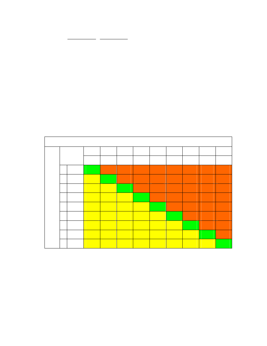
Table 2.1 shows how these probabilities are derived in a match Arsenal against
Liverpool at Highbury.
Probabilities for Liverpool with
λ
= 0.95
0 1 2 3 4 5 6 7 8
0.387 0.367 0.175 0.055 0.013 0.002 0.000 0.000 0.000
0 0.223 0.086 0.082 0.039 0.012 0.003 0.001 0.000 0.000 0.000
1 0.335 0.129 0.123 0.058 0.018 0.004 0.001 0.000 0.000 0.000
2 0.251 0.097 0.092 0.044 0.014 0.003 0.001 0.000 0.000 0.000
3 0.126 0.049 0.046 0.022 0.007 0.000 0.000 0.000 0.000 0.000
4 0.047 0.018 0.017 0.008 0.003 0.001 0.000 0.000 0.000 0.000
5 0.014 0.005 0.005 0.002 0.001 0.000 0.000 0.000 0.000 0.000
6 0.004 0.001 0.001 0.001 0.000 0.000 0.000 0.000 0.000 0.000
7 0.000 0.000 0.000 0.000 0.000 0.000 0.000 0.000 0.000 0.000
P
robabilitie
s
for
Ar
se
nal with
λ
=
1.
5
8 0.000 0.000 0.000 0.000 0.000 0.000 0.000 0.000 0.000 0.000
Table 2.1 Joint and marginal Poisson probabilities for all score combinations in a match Arsenal
versus Liverpool at Highbury with
λ
ARSENAL
= 1.5 and
λ
LIVERPOOL
= 0.95.
P(Arsenal win) = 0.497
P(Draw) = 0.261
P(Liverpool) = 0.236

26
Dixon and Coles reported that the model they were using enabled them to
establish a profitable betting strategy. In the other article “A birth process model
for association football matches” (1998), Dixon together with Robinson focused
on the spread betting market where the bets made “in running” were possible.
They observed that the rate of scoring goals varies over the course of a match and
concluded that inaccuracies exist in the spread betting market as well. Rue and
Salvesen (1997) continued Dixon’s footsteps by introducing the Poisson approach
in the Bayesian content. They applied Markov Chain Monte Carlo in order to
estimate the skills of all teams simultaneously. Application of the Poisson
distribution is also mentioned in Jackson’s (1994) article where he investigates
the similarities between the stock market and spread betting.
2.2 Alternative Prediction Schemes
Several team ratings have been proposed for different sports. In tennis, we are
familiar with ATP rankings, which measure the level of each player based on their
performances in the past. The betting line in American football is derived by
handicappers, who use power ratings as their basic tool. The basis of most of
these rating schemes is the least squares-Gaussian approach. Harville (1980) and
Stefani (1980) have published several articles on this subject. The main idea is to
predict the win margin in a match between two teams based on these previously
defined ratings. In Stefani’s article in Statistics in Sport journal (1998), he
proposes a least squares-Gaussian prediction system. He points out three steps in
his approach:
•
A rating is found for each team using win margin (score difference)
corrected for home advantage
•
The win margin is predicted for the next match using rating difference

27
•
The predicted win margin is used to estimate the probability of a home
win, draw and away win using the Gaussian distribution
The model has the following form:
i
j
i
i
e
h
r
r
z
+
+
−
=
Eq. 2.4
where z
i
represents the win margin for home team i in a match, h is an estimate of
the home advantage (one value for all teams), r
i
is the estimated rating for team i,
r
j
is the estimated rating for team j, and e
i
is a zero-mean random error due to
errors in estimating the ratings and home advantage plus random variation.
In order to estimate the probabilities of a home win, draw and away win,
thresholds t
1
and –t
2
are used where
)
(
)
(
)
(
)
(
)
(
)
(
2
1
2
1
t
z
P
Awaywin
P
t
z
t
P
Draw
P
t
z
P
Homewin
P
i
i
i
−
<
=
<
<
−
=
>
=
Eq. 2.5
The major difference between Maher-Poisson and least squares-Gaussian
approaches is that MP uses a discrete random variable, whereas LSG uses
continuous random variable.
2.2.1 Elo Ratings and Bradley-Terry Model
In chess, the most popular rating method is called Elo rating, named after the
inventor Arpad Elo (1978). The Elo rating system calculates a numerical rating
for every player based on performances in competitive chess. A rating is a
number normally between 0 and 3000 that changes over time depending on the
outcomes of tournament matches. When two players compete, the rating system

28
predicts the one with the higher rating to win more often. The more marked the
difference in ratings, the greater the probability that the higher rated player will
win according to Glickman and Jones (1999).
These Elo ratings can be applied to football as well. The probabilities for home
win, draw and away win are derived based on the difference in ratings. These
rating differences need to be stored over several years in order to examine how
often the match ends to a home win, a draw and an away win with various rating
differences. The ratings are updated by the following formula:
)
(
*
e
o
n
w
w
K
r
r
−
+
=
Eq. 2.6
where r
n
is the new rating, r
o
is the old (pre-match rating), K is the weight
constant depending on the league, normally 30. w is the result of the match (1 for
a win, 0.5 for a draw and 0 for a loss). w
e
is the expected result of the match (win
expectancy), either from the chart or from the following formula.
1
400
10
1
+
=
dr
e
w
Eq. 2.7
dr equals the difference in ratings plus 100 points for a team playing at home.
Initial ratings in Elo system are obtained by using a different set of formulas. The
resulting estimates are called “provisional ratings”. They do not carry a great
amount of confidence because they are based on a very small number of match
outcomes.
When a player has competed in fewer than 20 tournaments games, the post-
tournament rating is calculated based on all previous games, not just the ones in a
current tournament. The formula is

29
N
L
W
r
r
o
n
)
(
*
400
−
+
=
Eq. 2.8
where r
n
is the player’s post-tournament rating, r
o
is the average opponents’
ratings, W is the number of wins, L is the number of losses, and N is the total
number of games.
Glickman and Jones studied whether the winning expectancy formula could be
used to predict game outcomes between pairs of established players. Their main
conclusion was that there is a fair amount of variability in rating estimates. They
also discuss similar topics that arise in football including the time variation and
the problem of grouping.
In the US college soccer, the team rankings are created by Bradley-Terry model
(1952). Albyn Jones (1996) has an article about these on Internet. It follows
closely the Elo rating procedure. The Bradley-Terry model can be applied when
the response variable is binomial. The formula relating ratings to winning
probabilities is
))
(
exp(
1
))
(
exp(
a
h
a
h
R
R
R
R
P
−
+
+
−
+
=
β
α
β
α
Eq. 2.9
where P is the probability that the home team wins,
α
is a parameter representing
the home field advantage (specifically, it is the log odds for a home team victory
when the two teams are evenly matched), and
β
is a scale parameter chosen so
that a rating difference of 100 points corresponds to a probability of 2/3 of victory
for the higher rated team at a neutral site, ie.
00693
.
0
100
2
ln
≈
=
β

30
R
h
and R
a
are the home team rating and the away team rating, respectively.
For the 1995 NCAA men's and women's Division I teams, the home team wins
about 60% of the time, which corresponds to
α
= 0.405.
2.2.2 Multinomial Ordered Probit Model
Another LSG related method and more statistically acceptable than Elo ratings is
multinomial ordered logit/probit analysis. An article about ordered logit model by
Forrest and Simmons (2000) was used as a reference in our model comparison in
Chapter 3. Also, more theoretical articles by McCullach (1980) and Anderson
(1984) were applied.
Probit regression is an alternative log-linear approach in handling categorical
dependent variables. The outcome of a match, Win (2), Draw (1) or Loss (0) is
considered as a categorization of a continuous variable Z.
)
(
)
(
)
(
)
(
)
(
)
(
1
2
1
2
t
Z
P
Awaywin
P
t
Z
t
P
Draw
P
t
Z
P
Homewin
P
<
=
<
<
=
>
=
Eq. 2.10
Our probit model has the Normal Distribution with mean beta and variance 1. Z
is a normal random variable (ordered probit). The likelihood of the data is
calculated from P(Away win) = P(t
2
-
β
), where
β
= home team rating – away team
rating, and similarly for a draw and a home win. The cutpoints t
1
and t
2
are
estimated by maximizing the likelihood. The home effect is absorbed into the
estimates of t
1
and t
2
. If we had two equal strength teams r
i
= r
j
and the home
effect = 0, then we would have t
1
= -t
2.
The estimate for the home effect would be
½*(t
1
+t
2
). The probit version is thus very similar to the ratings, but parameters
and cutpoints are chosen in a statistical manner by the method of maximum
likelihood.

31
2.3 Betting
Strategies
The best and the most successful punters are money managers looking for ideal
situations, which are defined as matches with only high percentage of return. In
individual situations luck will play into the outcome of an event, which no amount
of odds compiling can overcome, but in the long run a disciplined punter will win
more of those lucky games than lose.
To achieve the level of profitable betting, one must develop a correct money
management procedure. The aim for a punter is to maximize the winnings and
minimize the losses. If the punter is capable of predicting accurate probabilities
for each match, the Kelly criterion has proven to work effectively in betting. It
was named after an American economist John L. Kelly (1956) and originally
designed for information transmission. The Kelly criterion is described below:
)
1
(
)
1
*
(
−
−
=
o
o
p
S
Eq. 2.11
where S = the stake expressed as a fraction of one’s total bankroll, p = probability
of an event to take place, o = odds for an event offered by the bookmaker. Three
important properties, mentioned by Hausch, Lo, and Ziemba (1994), arise when
using this criterion to determine a proper stake for each bet:
•
It maximizes the asymptotic growth rate of capital
•
Asymptotically, it minimizes the expected time to reach a specified goal
•
It outperforms in the long run any other essentially different strategy
almost surely

32
The criterion is known to economists and financial theorists by names such as the
geometric mean maximizing portfolio strategy, the growth-optimal strategy, the
capital growth criterion, etc. We will now show that Kelly betting will maximize
the expected log utility for a game, which uses biased coins.
2.3.1 Unconstrained Optimal Betting for Single Biased Coin
This section was derived based Thorp’s (1997) in-depth analysis about applying
the Kelly criterion in blackjack, sports betting and the stock market and Steve
Jacobs’ (1999) article about optimal betting. Consider an even money bet that is
placed on a biased coin which has a probability (p) of coming up heads and a
probability (1 - p) of coming up tails. If (p) is greater than 0.5, then a bet on heads
will be favorable for the player, and the player edge will be edge = P(winning) -
P(losing) = p - (1 - p) = 2p - 1.
If a fraction (f) of the current bankroll is wagered that the next flip of this coin
will come up heads, then the bankroll will increase by a factor of (1 + f) if the bet
is won, and the bankroll will shrink by a factor of (1 - f) if the bet is lost. If the
bankroll before the bet is B and log(B) is used as a utility function, then the
expected utility at the conclusion of this bet will be:
))
1
(
*
log(
*
)
1
(
))
1
(
*
log(
*
)
(
f
B
p
f
B
p
f
EU
−
−
+
+
=
Eq. 2.12
To find the optimal bet size for this coin toss, we must find the bet fraction, which
gives the maximum value for EU(f). We can find this value by solving:
0
)
(
=
df
f
dU
Eq.
2.13

33
0
)
1
(
*
*
)
1
(
)
1
(
*
*
=
−
−
−
+
⇒
f
B
B
p
f
B
B
p
Note that the absolute bankroll size B divides out and completely disappears from
the equation to give:
0
)
1
(
)
1
(
)
1
(
=
−
−
−
+
⇒
f
p
f
p
)
1
(
)
1
(
)
1
(
f
p
f
p
−
−
=
+
⇒
)
1
)(
1
(
)
1
(
f
p
f
p
+
−
=
−
⇒
pf
f
p
pf
p
−
+
−
=
−
⇒
1
f
p
p
+
−
=
⇒
1
1
2
−
=
⇒
p
f
Assuming (p > 0.5) so that betting on heads is a favorable bet, then (2p - 1) is
equal to the player edge for this coin flip. So, for a biased coin, one should bet a
fraction of bankroll that is equal to the advantage in order to maximize this utility
function. Notice that absolute bankroll size is unimportant.
One feature of sports betting which is of interest to Kelly users is the prospect of
betting on several games at once.

34
2.3.2 Unconstrained Optimal Betting for Multiple Biased Coins
Now suppose one is playing a game where there are 4 different coins (A, B, C,
D). The probabilities of these coins being played are (pA, pB, pC, pD), and the
probability of these coins coming up heads are (hA, hB, hC, hD). Before any
game is played, the player is shown which coin is to be flipped so that he/she can
choose a different bet size for different coins. Again, one wants to find a betting
strategy (fA, fB, fC, fD) which will maximize the expected utility, using
log(bankroll) as a utility function.
The overall utility (OU) function for this game is simply a weighted sum of the
utility functions for each of the individual coins. Each coin contributes an amount
to the overall utility, which is proportional to the probability of that coin being
played. So,
)
(
*
)
(
*
)
(
*
)
(
*
)
,
,
,
(
fD
EU
pD
fC
EU
pC
fB
EU
pB
fA
EU
pA
fD
fC
fB
fA
OU
+
+
+
=
Eq. 2.14
))
1
log(
*
)
1
(
)
1
log(
*
(
*
fA
hA
fA
hA
pA
−
−
+
+
⇒
))
1
log(
*
)
1
(
)
1
log(
*
(
*
fB
hB
fB
hB
pB
−
−
+
+
+
))
1
log(
*
)
1
(
)
1
log(
*
(
*
fC
hC
fC
hC
pC
−
−
+
+
+
))
1
log(
*
)
1
(
)
1
log(
*
(
*
fD
hD
fD
hD
pD
−
−
+
+
+
Maximizing the OU for one of the bet sizes fa gives
0
))
(
(
=
dfA
fA
OU
d
Eq. 2.15
0
))
(
(
*
=
⇒
dfA
fA
EU
d
pA

35
which holds when
0
))
(
(
=
⇒
dfA
fA
EU
d
This is the same equation used to optimize a single coin toss. The important thing
to notice here is that the optimum bet size for fA does not depend on pA, so it
does not matter how often coin A is played. So, when playing coin A, one simply
should play as if that was the only coin in the game, and one should choose the
correct bet size for that coin.
2.3.3 More on Kelly Criterion
The problem of using this Kelly criterion is that generally only estimates of the
true probabilities are available, whereas Kelly criterion assumes that the true
probabilities are known. Instead of maximizing the capital growth, strategies can
be developed based on maximum security. For instance, probability of ruin can
be minimized subject to making a positive return, or confidence levels can be
computed of increasing initial fortune to a given final wealth goal. To combine
the goals of capital growth and security, an alternative is a fractional Kelly
criterion, i.e. compute the optimal Kelly investment but invest only a fixed
fraction of that amount. Thus security can be gained at the price of growth by
reducing the investment fraction.
How does Kelly criterion compare with other strategies over a time period?
Hausch, Lo and Ziemba conducted a study of 1000 trials, or horse racing seasons,
each of 700 races, assuming the initial wealth of $1000. The Kelly criterion is
compared to the fractional Kelly criterion with the fraction ½. Also, in
consideration are 1) “fixed” bet strategies that establish a fixed bet regardless of

36
the probability of winning, the bet’s expected return, or current wealth; and 2)
“proportional” bet strategies that establish a proportion of current wealth to bet
regardless of the circumstances of the wager. The results are presented in
Appendix C.
The simulation provides support for Kelly system, even over a horizon as short as
one racing season. Some punters may find the distributions of final wealth from
other systems may be more appealing for this period, e.g. a fractional Kelly
system for a more conservative punter. In this thesis, we compare fixed stake, full
Kelly, ½ Kelly and ¼ Kelly.

37
Chapter 3
3 Data Description and Model Formulation
3.1 Data Description
Data has been collected over the last four seasons in the English Premier League.
These include 1997-1998, 1998-1999, 1999-2000 and 2000-2001 seasons. We
have also collected the season 2000-2001 data from the main European football
betting leagues, such as English Division 1, Division 2 Division 3, Italian Serie A,
German Bundesliga and Spanish Primera Liga. The data source was the website
sunsite.tut.fi/rec/riku/soccer2.html. This website records only dates, matches and
results. A large amount of extra information of league football like goal scorers,
times when the goals were scored, line-ups, attendances is available in other
portals, but we are not using these in our study. In practice, it would be difficult
to use more general information in a numerical format. Therefore, in the basic
model our input is each team’s history of match scores (following Maher and
Dixon). We also include dates in our analysis to examine the hypotheses that
more recent results are better indicator of teams’ current form. Later, we also
make an extension to apply the odds data in our analysis. Bookmaker’s odds were
obtained from the website oddscomparison.com.
Due to the relegations and promotions, teams change from season to season.
Each year, there are three new teams in the league replacing the last year’s bottom
three. We used the data from the seasons 1997-2000 to test the validity of
Poisson and independence assumptions. Three seasons of data means 1140 full-
time match scores. In building the betting strategy and testing the model’s
efficiency, we focus on the most recent season, which is 2000-2001. We use

38
bookmakers’ odds from the 2000-2001 season as our validation sample, to
investigate the possibility of a profitable betting strategy.
3.2 Poisson Regression Formulation
3.2.1 Assumptions
As the lambdas vary from match to match, there is no direct way to test he
validity of the Poisson assumption (no replicates). However, we can assess
whether the assumption holds in an average sense. Below, we have summary
statistics and histograms to demonstrate the distribution of home and away goals
in the Premier League 1997-2000.
*** Summary Statistics ***
Home.goals Away.goals
Min:
0 0
Mean:
1.56 1.10
Median: 1 1
Max:
8 8
Total N:
1140 1140
Std Dev: 1.35 1.16
Table 3.1 Summary statistics
of home and away goals in 1140 matches in the English Premier
League 1997-2000.
39
0
50
100
150
200
250
300
350
400
0
1
2
3
4
5
6
7
8
9
Number of goals
Histogram of home goals
Actual
Poisson
Figure 3.1
Histogram of the number of home goals in 1140 matches in the English Premier
League 1997-2000 vs. Poisson approximations with λ
HOME
= 1.56 and λ
AWAY
= 1.10.
0
50
100
150
200
250
300
350
400
450
0
1
2
3
4
5
6
7
8
9
Number of goals
Histogram of away goals
Actual
Poisson
Figure 3.2 Histogram of the number of away goals in 1140 matches in the English Premier
League 1997-2000 vs. Poisson approximations with λ
HOME
= 1.56 and λ
AWAY
= 1.10.

40
Dixon and Coles concluded from their dataset, which included the seasons 1993-
1995 that Poisson assumption had a nearly perfect fit except for the scores 0-0, 1-
0, 0-1 and 1-1. They made an adjustment in their likelihood function, where they
included a coefficient allow for the departure from the independence assumption.
It interferes the traditional likelihood function procedure, and thus they are forced
to use a so-called “pseudo-likelihood”. We are not considering this slight
departure from the independence any further in a proper statistical manner due to
its complexity in calculations. Instead we suggest an ad hoc approach later in this
chapter.
Test statistic for the standard chi-squared test is calculated in the following way:
∑∑
=
=
−
=
m
i
ij
ij
ij
n
j
E
E
O
1
2
1
2
)
(
χ
Eq. 3.1
Away goals
0 1 2 3 4 5 6 8
0
7.38 0.06 1.40 0.61 3.51 0.80 0
0
1
0.17 0.45 3.09 0.09 0.76 1.06 0
0
2
0.84 0.02 1.29 0.95 0.14 0.37 0
0
3 1.77
1.62
0.07
3.01
4.99
0 0 0
4 4.41
0.08
1.28
0.03
0.53
0 0 0
5 7.66
0.23
0.79
0.09
0 0 0 0
6 0.10
0.32
0 0 0 0 0 0
Hom
e goals
7 0 0 0 0 0 0 0 0
Table 3.2 Chi-square table where the cells whose expected count is less than 1 are deleted.
If we sum up all the cells our test statistic will be 50.08. We have here 34 valid
cells (>1), so our degrees of freedom will be 34-2 = 32. Corresponding p-value is

41
2.2%, which denotes that it is significant. Therefore, we reject our null
hypothesis and conclude that scores are not Poisson. Despite this, we adopt to use
the Poisson assumption in our model. The big chi-square values for certain
combination of scores (0-0, 4-0, 5-0) affect the test statistic quite heavily. These
departures probably arise from non-independence. In a low-scoring match (0-0)
both teams normally will focus on defence in the latter stages of the match, and
thus the probability of a 0-0 result increases. Runaway victories (4-0, 0-5) take
place when the losing team gives up (or the winning team has a psychological
advantage). Hence the probability of heavy defeats is higher than would be
expected under the Poisson model. The closer comparison of empirical and
model probabilities over three seasons of English Premier League is presented in
Tables 3.9 and 3.10.
3.2.2 Basic Model
With the basic model we want to establish the validity of the model. The reason
for using Poisson regression is because we are modelling goals scored, which is
discrete data. The S-Plus output of the regression is provided below. The data for
this particular regression covers the whole season 1999-2000.
*** Generalized Linear Model ***
Coefficients:
Arsenal.att=0
Value Std. Error t value
home 0.401535082 0.06263281 6.410938645
aston.villa.att -0.470757637 0.18837348 -2.499065305
bradford.att -0.629751325 0.20015584 -3.146305011
chelsea.att -0.329852673 0.18063382 -1.826084764
coventry.att -0.430567731 0.18714373 -2.300732931
derby.att -0.493712494 0.19094065 -2.585685575
everton.att -0.207546257 0.17526624 -1.184177037
leeds.att -0.230658918 0.17608878 -1.309901296
leicester.att -0.271955423 0.17876504 -1.521300938
liverpool.att -0.372273136 0.18262428 -2.038464623
manchester.u.att 0.287397732 0.15522209 1.851525926
middlesbrough.att -0.454107452 0.18842902 -2.409965634
newcastle.att -0.136720214 0.17220709 -0.793929084
sheffield.w.att -0.627736511 0.19987443 -3.140654422

42
southampton.att -0.466210345 0.18975938 -2.456850029
sunderland.att -0.235122947 0.17699582 -1.328409612
tottenham.att -0.242130272 0.17698025 -1.368120318
watford.att -0.703210028 0.20582698 -3.416510423
west.ham.att -0.330203468 0.18165843 -1.817716171
wimbledon.att -0.432099261 0.18851518 -2.292119171
arsenal.def 0.234691351 0.19847950 1.182446307
aston.villa.def 0.001673309 0.20664415 0.008097541
bradford.def 0.659300496 0.16991936 3.880078724
chelsea.def -0.020542641 0.20854554 -0.098504341
coventry.def 0.437138168 0.18076508 2.418266687
derby.def 0.488365345 0.17801844 2.743341402
everton.def 0.351658946 0.18584990 1.892166421
leeds.def 0.219696626 0.19334585 1.136288304
leicester.def 0.463510484 0.17981968 2.577640421
liverpool.def -0.147852987 0.21783909 -0.678725683
manchester.u.def 0.304878683 0.19053565 1.600113608
middlesbrough.def 0.398317734 0.18268388 2.180366065
newcastle.def 0.453146988 0.18068667 2.507916054
sheffield.w.def 0.688363506 0.16868874 4.080672640
southampton.def 0.573662574 0.17401039 3.296714565
sunderland.def 0.483591947 0.17889362 2.703237456
tottenham.def 0.349661870 0.18588592 1.881056234
watford.def 0.780925968 0.16480591 4.738458411
west.ham.def 0.423367627 0.18166460 2.330490561
wimbledon.def 0.752147908 0.16636701 4.521015975
(Dispersion Parameter for Poisson family taken to be 1)
Null Deviance: 1088.126 on 760 degrees of freedom
Residual Deviance: 820.8908 on 720 degrees of freedom
Table 3.3 S-Plus output of the Poisson regression.

43
Team
M W D L GF
GA
Pts
.att
.def
1.
Manchester_U
38 28 7 3 97 45 91
0.29
0.30
2.
Arsenal
38 22 7 9 73 43 73
0.00
0.23
3.
Leeds
38 21 6 11 58 43 69 -0.23
0.22
4.
Liverpool
38 19 10 9 51 30 67 -0.37 -0.15
5.
Chelsea
38 18 11 9 53 34 65 -0.33 -0.02
6.
Aston_Villa
38 15 13 10 46 35 58 -0.47
0.00
7.
Sunderland
38 16 10 12 57 56 58 -0.24
0.48
8.
Leicester
38 16 7 15 55 55 55 -0.27
0.46
9.
West_Ham
38 15 10 13 52 53 55 -0.33
0.42
10.
Tottenham
38 15 8 15 57 49 53 -0.24
0.35
11.
Newcastle
38 14 10 14 63 54 52 -0.14
0.45
12.
Middlesbrough
38 14 10 14 46 52 52 -0.45
0.40
13.
Everton
38 12 14 12 59 49 50 -0.21
0.35
14.
Coventry
38 12 8 18 47 54 44 -0.43
0.44
15.
Southampton
38 12 8 18 45 62 44 -0.47
0.57
16.
Derby
38 9 11 18 44 57 38 -0.49
0.49
17.
Bradford
38 9 9 20 38 68 36 -0.63
0.66
18.
Wimbledon
38 7 12 19 46 74 33 -0.43
0.75
19
Sheffield_W
38 8 7 23 38 70 31 -0.63
0.69
20.
Watford
38 6 6 26 35 77 24 -0.70
0.78
Table 3.4 Final league table of 1999-2000 season together with attack and defence parameters.
In a regular regression procedure variables with small t-values would be deleted.
In our study it would not make sense, since we need to have an estimate for each
team’s attack and defence qualities. When we observe the final league table and
the attack and defence parameters, we notice that they are closely related.
Arsenal’s attack parameter is set to zero as our base parameter. Among attack
parameters, the larger value represents more effective attack. From Table 3.4 we
see that Manchester United is the only team, which has stronger attack parameter
than Arsenal. This statement is also supported by the amount of goals scored.
Manchester United scored 97 goals (GF column), which is the best in the league.
Among defensive parameters the smaller value means better defence. Liverpool
has the best defence parameter value (-0.15), while Watford has the worst (0.78).
This agrees with the league table when we observe the goals allowed (GA)
column. The correlation matrix in Table 3.5 describes that there is a strong
correlation between model parameters and goals scored and allowed.
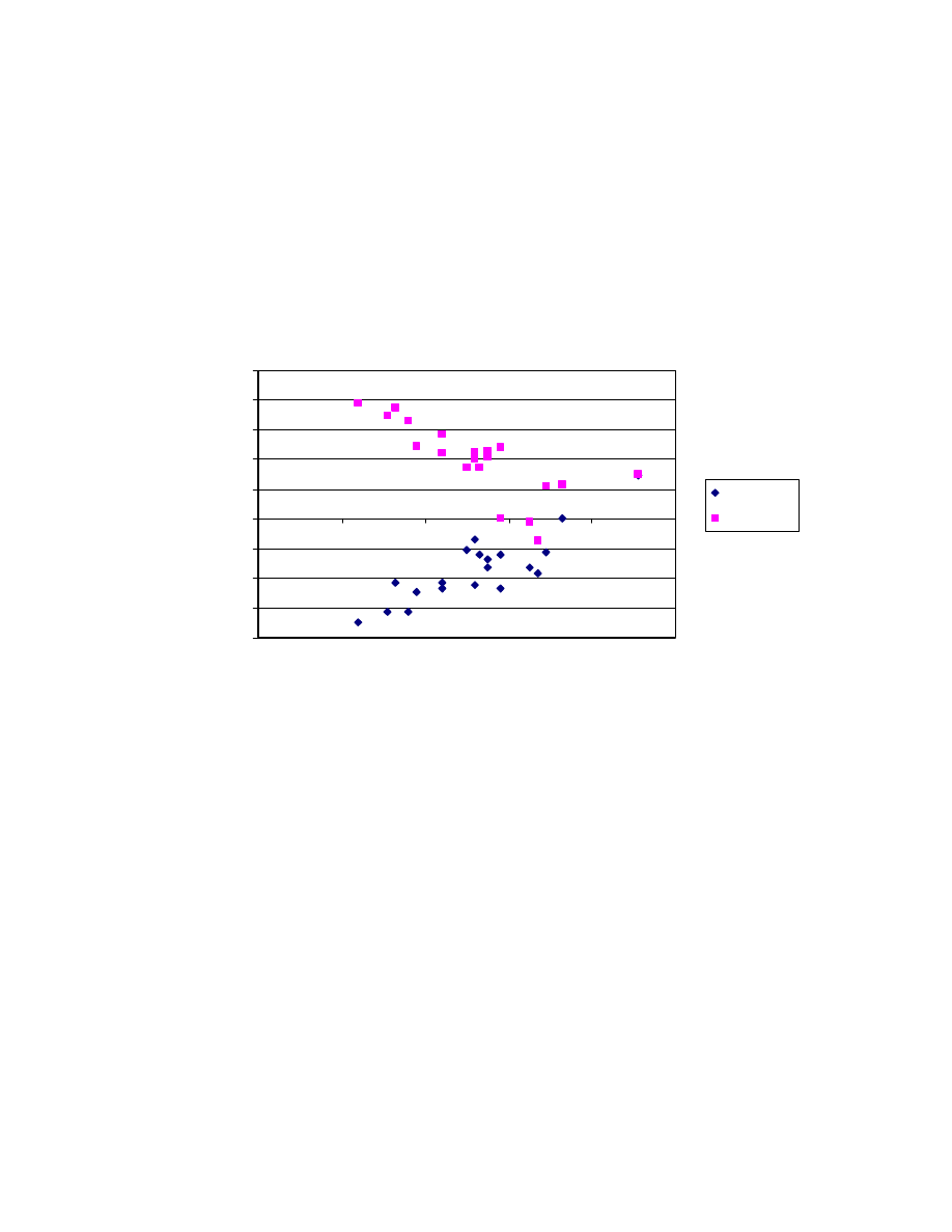
44
*** Correlations ***
Goals.for Goals.allowed Points .att .def
Goals.for 1.0000000 -0.4751649 0.8517034 0.9872455 -0.3705375
Goals.allowed -0.4751649 1.0000000 -0.8056237 -0.5107841 0.9844414
Points 0.8517034 -0.8056237 1.0000000 0.8545026 -0.7387740
.att 0.9872455 -0.5107841 0.8545026 1.0000000 -0.3991579
.def -0.3705375 0.9844414 -0.7387740 -0.3991579 1.0000000
Table 3.5 Correlation matrix of the data in Table 3.4.
League points vs. Attack/Defence
-0.8
-0.6
-0.4
-0.2
0
0.2
0.4
0.6
0.8
1
0
20
40
60
80
100
League points
Par
am
et
er
est
im
at
e
Attack
Defence
Figure 3.3 Scatter plot of attack and defence parameters vs. league points.
Our interest was to model goals and therefore we need to see how well we were
able to do that. If we sum up the lambdas derived using the model and compare
that to actual number of goals both home and away, we get the estimates below:
Home goals Away goals
Model
633
433
Actual
635
425
This table was constructed for the full 1999-2000 season dataset. It demonstrates
that the Poisson model reasonably reflects some basic features of the data. That is

45
encouraging especially for correct score and spread betting purposes. In the fixed
odds surroundings, we need to see how the outcome probabilities reflect the
actual ones. If we calculate the average of these model probabilities over three
seasons we get the following numbers:
Model
Actual
1
X
2
1
X
2
99-00 .49 .23 .28
.49 .24 .27
98-99 .46 .25 .29
.45 .30 .25
97-98 .47 .24 .29
.48 .25 .27
When we compare the model to the actual values we get quite satisfactory results.
In reality we do not have the whole season data available when placing the bet.
We examine that problem in later sections. With the basic model we just want to
prove the usefulness of the model.
The model validation in regression is normally done by observing the fitted values
and the residuals from the model. For the basic model, the residual analysis done
by Minitab gives the following results:
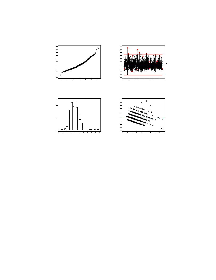
46
Figure 3.4 Minitab output of the residual analysis.
The graphs indicate that response residuals are reasonable normally distributed
with few outliers. There is a risk that these few outliers may overestimate certain
teams’ attacking power and underestimate the opponents’ defensive ability. This
happens in a match where unusually many goals are scored. For instance,
Sunderland achieved few heavy away victories on the first half of the season.
They beat Derby 0-5 and Bradford 0-4. Those victories weighted quite heavily
also later in the season. They are not significant outliers though. If the team gets
beaten, let’s say 10-0, we need to consider some modifications to the analysis.
We now consider alternative models in order to choose the best available model
for our prediction process.
6
5
4
3
2
1
0
-1
-2
-3
-4
100
50
0
Residual
Fr
eq
ue
nc
y
Histogram of Residuals
800
700
600
500
400
300
200
100
0
6
5
4
3
2
1
0
-1
-2
-3
-4
Observation Number
R
es
id
ual
I Chart of Residuals
6
1
1
2
5
8
8
6
1
1
5
1
22
2
277
7
7
7
7
77
5
77
7
7
7
7
7
7
5
7
777
6
X=0.000
3.0SL=3.378
-3.0SL=-3.378
4.5
4.0
3.5
3.0
2.5
2.0
1.5
1.0
0.5
0.0
6
5
4
3
2
1
0
-1
-2
-3
-4
Fit
R
es
idu
al
Residuals vs. Fits
3
2
1
0
-1
-2
-3
6
5
4
3
2
1
0
-1
-2
-3
-4
Normal Plot of Residuals
Normal Score
R
e
si
du
al
Residual Model Diagnostics

47
3.2.3 Separate Home Parameter Model
The existence of a home advantage is well documented in many sports. The more
comprehensive analysis on subject is found in the article by Clarke and Norman
(1995). A common method to estimate home advantage is to divide the number
of points accomplished at home by the total number of points received over the
whole season. The result of that is given in Table 3.6 over three seasons 1996-
1999. Earlier in the English league, the teams who played on the artificial ground
earned a significant home advantage. These teams were QPR, Luton and Preston
in the 1980’s. Nowadays, artificial fields are prohibited. In our study, we want to
see whether the home advantage varies significantly from team to team. Is there a
need to include a separate home parameter for each team into our model?
98-99
97-98
96-97
1 Manchester_U 0.582
1 Arsenal
0.602
1 Manchester_U 0.546
2 Arsenal
0.602
2 Manchester_U 0.558
2 Newcastle
0.617
3 Chelsea
0.560
3 Liverpool
0.630
3 Arsenal
0.514
4 Leeds
0.611
4 Chelsea
0.650
4 Liverpool
0.529
5 West_Ham
0.631
5 Leeds
0.542
5 Aston_Villa
0.622
6 Aston_Villa
0.600
6 Blackburn
0.637
6 Chelsea
0.593
7 Liverpool
0.648
7 Aston_Villa 0.526
7 Sheffield_W
0.596
8 Derby
0.596
8 West_Ham
0.767
8 Wimbledon
0.589
9 Middlesbrough 0.588
9 Derby
0.709
9 Leicester
0.553
10 Leicester
0.551 10 Leicester
0.528 10 Tottenham
0.608
11 Tottenham
0.595 11 Coventry
0.634 11 Leeds
0.608
12 Sheffield_W
0.565 12 Southampton
0.645 12 Derby
0.652
13 Newcastle
0.586 13 Newcastle
0.659 13 Blackburn
0.666
14 Everton
0.604 14 Tottenham
0.659 14 West_Ham
0.642
15 Coventry
0.714 15 Wimbledon
0.477 15 Everton
0.595
16 Wimbledon
0.666 16 Sheffield_W
0.727 16 Southampton
0.609
17 Southampton
0.756 17 Everton
0.650 17 Coventry
0.487
18 Charlton
0.527 18 Bolton
0.725 18 Sunderland
0.675
19 Blackburn
0.657 19 Barnsley
0.714 19 Middlesbrough 0.743
20 Nottingham
0.533 20 Crystal_P
0.333 20 Nottingham
0.529
Mean
0.608
Mean
0.619
Mean
0.599
Standard
Error
0.012
Standard
Error
0.022
Standard
Error
0.013
Median
0.598
Median
0.641
Median
0.602
Mode
#N/A
Mode
0.659
Mode
0.529
Standard
Deviation 0.057
Standard
Deviation 0.101
Standard
Deviation 0.061
Range
0.228
Range
0.434
Range
0.255
Minimum
0.527
Minimum
0.333
Minimum
0.487
Maximum
0.756
Maximum
0.767
Maximum
0.743

48
Sum
12.17
Sum
12.38
Sum
11.98
Count
20
Count 20
Count 20
Table 3.6 The ratio of the number points accomplished at home per the total number of points
over three seasons including summary statistics.
We observe that relatively high variability existed during the season 1997-1998.
That is explained by Crystal Palace’s performance. They received only 33% of
the total points at home. This must be one of the worst records in the history of
English football. Other than that, the home effect seems to be relatively constant.
A Poisson regression with different home parameters was fitted with following
home parameter values. The full regression output is in Table D.1 in Appendix
D.
Team
Coefficient Ratio
1 manchester.u.home
0.1362689
0.53846
2 arsenal.home
0.3036824
0.61644
3 Leeds.home
-0.303683
0.55072
4 liverpool.home
-0.106972
0.55224
5 chelsea.home
0.361294 0.63077
6 aston.villa.home -0.303683
0.55172
7 sunderland.home -0.338774
0.62069
8 leicester.home
-0.047749
0.6
9 West.ham.home
0.1663202
0.69091
10 tottenham.home
0.5519839 0.62264
11 newcastle.home
0.3894649 0.67308
12 middlesbrough.home
-0.303682 0.55769
13 everton.home
0.1443425 0.6
14 coventry.home
1.1366615 0.84091
15 southampton.home 0.0099749 0.63636
16 derby.home
-0.30368 0.55263
17 bradford.home
0.4694657 0.72222
18 wimbledon.home
0.3249246 0.75758
19 sheffield.w.home -0.092371 0.67742
20 watford.home
0.4764658 0.79167
Table 3.7 Comparison of the model parameters and the ratio estimate of points at home and total
points for season 1999-2000.
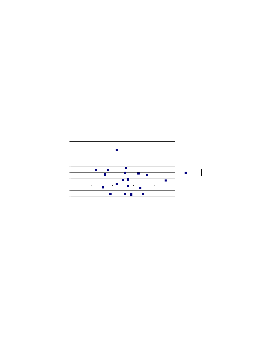
49
*** Correlations ***
.home ratio
home 1.0000000 0.7717654
ratio 0.7717654 1.0000000
Table 3.8 Correlation matrix of data given in Table 3.7.
We notice that the values form the model somewhat correspond to the ratio
estimates. It indicates that Coventry received most of their points at home. Either
they had a particularly good home advantage or they underperformed in away
matches. We can observe this further by scatter plot.
League points vs. home effect
-0.6
-0.4
-0.2
0
0.2
0.4
0.6
0.8
1
1.2
1.4
0
20
40
60
80
100
League points
P
a
ra
m
e
ter
esti
m
ate
Home
Figure 3.5 Scatter plot of league points vs. home effect.
The outlier represents Coventry’s home record. We leave the conclusion of
including different home parameters to our model in Section 3.2.6.

50
3.2.4 Split Season Model
Another possibility is that the parameters change over the season. We tested this
by considering a split season model. The interest is to find out whether the first
half of the season is different from the second half.
From the reports in Appendix D we see how certain teams’ performance varied
greatly during the separate halves of the season. Sunderland, for example, did
noticeably worse on the second half than on the first half. Their attack parameter
decreased from –0.013 to -0.522 and defence parameter increased from 0.261 to
0.747. This explains their change in position dropped heavily after Christmas.
These values depend on the assumption that Arsenal’s attack parameter remained
constant in both halves of the season. Home effect does not seem to change that
much. Complete S-Plus reports are documented in Table D.2 and D.3 in
Appendix D.
3.2.5 Comparison among Poisson Models with Full Season Data
The comparison between two Poisson models is done by observing their residual
deviances. We can also apply the log-likelihood ratio statistic as described by
Bishop, Frienberg and Holland (1975):
[
]
∑
=
=
−
=
N
i
i
i
i
e
y
y
y
b
y
b
l
D
1
max
log
2
)
;
(
)
;
(
2
Eq. 3.2
If the model fits the data well, then for large samples D has the central chi-
squared distribution with degrees of freedom given by the number of cells with
non-zero observed frequencies minus the number of independent, non-zero
parameters in the model. Below we have the residual deviances and the
corresponding degrees of freedom between different Poisson regression models.

51
Model
Residual
Deviance
df
Basic
820.89
720
Different
home
parameters
791.88
701
Separate
halves 786.53
680
1
st
half 392.87
340
2
nd
half 393.66
340
Test of hypothesis to observe whether any significant difference exists between
models was constructed. The results are below:
Model
Diff. Deviance
df
p-value
Basic vs. Different home parameters
29.01
19
0.06
Basic
vs.
Separate
halves
34.36
40
0.72
We can conclude that the Basic model produces an adequate fit and none of the
modifications above are necessary.
3.2.6 Odds Data and E(Score) Model
We can incorporate the odds data into our model by converting the odds to the
expected scores according to the Poisson distribution. The data source for odds is
oddscomparison.com and the odds are converted to expected scores by using
Excel Solver add-in. We make an assumption that the bookmaker’s forecast
should have the same accuracy for home and away teams. Again, following the
Section 2.1 this is a simplified notation of the model.
Log (
λ
HOME
)
=
β
HOME
* z
1
+
β
E(Score)
* z
2
+
β
HOMEATTACK
* z
3
+
β
AWAYDEFENCE
* z
4
Log (
λ
AWAY
) =
β
E(Score)
* z
5
+
β
AWAYATTACK
* z
6
+
β
HOMEDEFENCE
* z
7
Eq.
3.3
Log (E(Y)) =
β
HOME
* z
1
+
β
E(Score)
* z
2
+
β
HOMEATTACK
* z
3
+
β
AWAYDEFENCE
* z
4
+
β
E(Score)
* z
5
+
β
AWAYATTACK
* z
6
+
β
HOMEDEFENCE
* z
7
Eq. 3.4
where
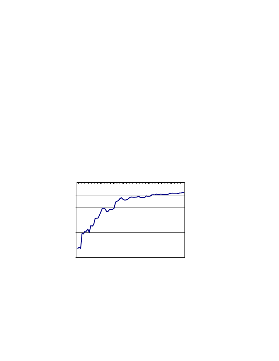
52
z
1
= 1 if Y refers to goals scored by home team
= 0 if Y refers to goals scored by away team;
z
2
= Log(E(home score)) derived from the bookmaker odds if Y refers to goals
scored by home team
= 0 if Y refers to goals scored by away team;
z
3
= 1 if Y refers to goals scored by home team
= 0 if Y refers to goals scored by away team;
z
4
= 1 if Y refers to goals scored by home team
= 0 if Y refers to goals scored by away team;
z
5
= Log(E(away score)) derived from the bookmaker odds if Y refers to goals
scored by away team
= 0 if Y refers to goals scored by home team;
z
6
= 0 if Y refers to goals scored by home team
= 1 if Y refers to goals scored by away team;
z
7
= 0 if Y refers to goals scored by home team
= 1 if Y refers to goals scored by away team.
If we fit the model for the season 2000-2001 and observe how the
β
E(Score)
parameter behaves.
E(Score)
-6.00
-5.00
-4.00
-3.00
-2.00
-1.00
0.00
1
7
13
19
25
31
37
43
49
55
61
67
73
Time (days)
P
ar
amet
er
est
im
at
e
Figure 3.6 Time series for
β
E(Score)
parameter.
β
E(Score)
parameter seems to converge towards the value –0.8. We include this
model in our comparison to find the best available Poisson model.

53
3.2.7 Poisson Correction Model
Empirical probabilities of all combinations of goals scored by home and away
teams over three seasons appear in Table 3.9.
Away goals
0 1 2 3 4 5 6 8
36.05 35.00 17.89 7.63 2.37 0.53 0.44 0.09
0 25.09 10.79 7.37 4.39 1.75 0.61 0.09 0.09 0.00
1 32.46 11.23 11.67 5.35 2.81 0.88 0.26 0.18 0.09
2 22.81 7.19 8.95 5.00 0.88 0.44 0.18 0.18 0.00
3 11.58 3.60 4.30 1.84 1.40 0.44 0.00 0.00 0.00
4 5.18 1.93 1.67 0.96 0.61 0.00 0.00 0.00 0.00
5 1.84 1.05 0.61 0.09 0.09 0.00 0.00 0.00 0.00
6 0.61 0.18 0.18 0.18 0.09 0.00 0.00 0.00 0.00
Hom
e goals
7 0.44 0.09 0.26 0.09 0.00 0.00 0.00 0.00 0.00
Table 3.9 Empirical marginal and joint probabilities for each combination of scores.

54
Away goals
0 1 2 3 4 5 6 8
33.29 36.62 20.14 7.38 2.03 0.45 0.08 0.00
0 21.01 6.99 7.70 4.23 1.55 0.43 0.09 0.02 0.00
1 32.78 10.91 12.00 6.60 2.42 0.67 0.15 0.03 0.00
2 25.57 8.51 9.36 5.15 1.88 0.52 0.11 0.02 0.00
3 13.30 4.42 4.87 2.68 0.98 0.27 0.06 0.01 0.00
4 5.19 1.73 1.90 1.04 0.38 0.11 0.02 0.00 0.00
5 1.62 0.54 0.59 0.33 0.12 0.03 0.00 0.00 0.00
6 0.42 0.14 0.15 0.08 0.03 0.00 0.00 0.00 0.00
Hom
e goals
7 0.09 0.03 0.03 0.02 0.00 0.00 0.00 0.00 0.00
Table 3.10 Estimated ratios of the joint probability and the marginal probability functions under
the assumption of independence with
λ
HOME
= 1.56 and
λ
AWAY
= 1.10.
We can incorporate the Poisson and dependence correction to our model in an ad
hoc way by multiplying each cell by the ratio of the empirical and average model
values from the above tables in the following way.
)
,
(
*
)
,
(
)
,
(
)
,
(
j
i
Model
j
i
AvgModel
j
i
Empirical
j
i
rection
PoissonCor
=
Eq.3.5
where
Empirical(i,j) = value from Table 3.9
AvgModel(i,j) = value from Table 3.10
Model(i,j) = value from the model
PoissonCorrection(i,j) = corrected value
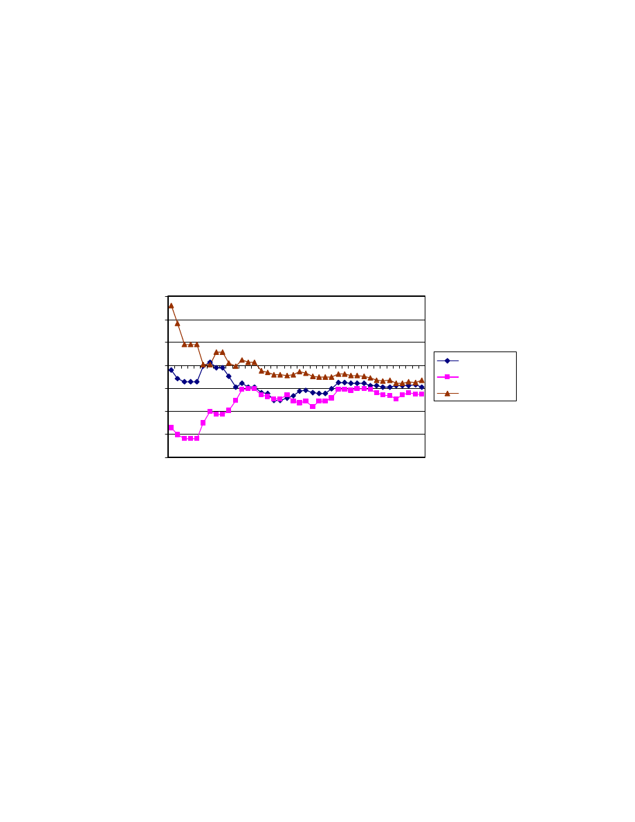
55
3.2.8 Weighted Model
To place more emphasis on more recent matches we consider weighted model.
That could be useful in order to give better information about the teams’ current
forms. The week-by-week fitted time series charts show how the betas for
particular teams vary over the season. It also shows how the home effect remains
nearly constant.
Attack
-2
-1.5
-1
-0.5
0
0.5
1
1.5
1
4
7
10
13
16
19
22
25
28
31
34
37
40
Time (weeks)
P
a
ra
m
e
ter
esti
m
ate
Aston Villa
Bradford
Chelsea
Figure 3.7 Time series of the maximum likelihood estimates of attack parameters for Aston Villa,
Bradford and Chelsea.
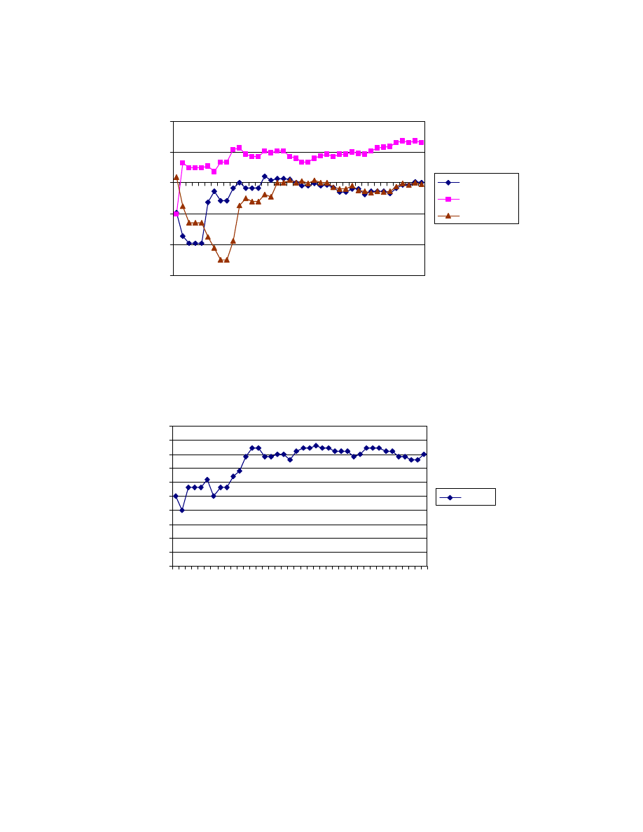
56
Defence
-1.5
-1
-0.5
0
0.5
1
1
4
7
10
13
16
19
22
25
28
31
34
37
40
Time (weeks)
P
a
ra
m
e
ter
esti
m
ate
Aston Villa
Bradford
Chelsea
Figure 3.8 Time series of the maximum likelihood estimates of defence parameters for Aston
Villa, Bradford and Chelsea.
Home effect
0
0.05
0.1
0.15
0.2
0.25
0.3
0.35
0.4
0.45
0.5
1
4
7
10
13
16
19
22
25
28
31
34
37
40
Time (weeks)
P
a
ra
m
e
ter
esti
m
ate
Home
Figure 3.9
Time series of the maximum likelihood estimate of home parameter.
These charts were constructed on a week-by-week updating scheme. Attack and
defence charts were done for three teams in the Premiership season 1999-2000:
Aston Villa, Bradford and Chelsea. It indicates that in the first few weeks of the

57
season the parameters are highly variable. After approximately 10 weeks of the
season, parameters start to stabilize, because more data is available. The home
effect behaves in a similar manner, but with less variation than attack and defence
parameters. We conclude that the basic model in this format is useful after the
10
th
week of the season. In order to estimate the early weeks of the season, we
could apply expert opinions, which are derived from odds data. That aspect is
described later in this chapter.
The definition of a weight function is discussed in the article published by Dixon
and Coles, where they suggested the exponential weight function. We suggest
that half normal distribution could be better to emphasize the most recent results
even more heavily.
)
)
(
*
exp(
2
0
t
t
a
tion
WeightFunc
−
=
Eq. 3.6
where a = half normal distribution parameter, t = particular day of the season and
t
0
= starting day of the season. The weighted regression output run for the full
season dataset is documented in Table D.4 in Appendix D.
The parameter estimation for our half normal distribution is not straightforward.
From Table 3.11 we selected a value -0.000007 for our weight function parameter
after trial and error.

58
Weight parameter Deviance
-0.0005
900.89
-0.00005
833.83
-0.00003
826.17
-0.00002
822.06
-0.00001
819.43
-0.000009
819.32
-0.000007
819.27
-0.000006
819.33
-0.000005
819.43
Table 3.11 The trial and error results for the weight parameter.
In the next section, we make a comparison between the weighted regression and
unweighted regression to see whether we get any improvement with weighting.
3.3 Comparison among Poisson Models Week-by-week
Because the dataset is constantly changing, due to the new matches, we do not
have the whole season dataset when placing a bet. Therefore, the basic model for
the full season data gives the better results than in reality it would be possible.
We can only include the matches played up to the present date. If we calculate
the average of these model probabilities over three seasons by updating the data
on a week-by-week basis, we get the following numbers:
1 X
2
99-00 .49 .23 .28
98-99 .45 .26 .29
97-98 .47 .24 .29

59
This compared to the actual average probabilities of these seasons, which are:
1 X
2
99-00 .49 .24 .27
98-99 .45 .30 .25
97-98 .48 .25 .27
Here we see that the fit of the model looks at least adequate in an average sense.
One weakness is that the probability of a draw is a little bit underestimated and
the away win overestimated. This is mainly due to the Poisson assumption. In
order to adjust that, it is possible to use methods of Dixon and Coles or the
Poisson Correction method described in Section 3.2.7. By running the regression
on a week-by-week basis, we get approximately 40 different regression outputs.
Thus, comparison of residual deviances to alternative models is not
straightforward. The graph below describes the Poisson models we chose for
closer look.
Poisson Models
Figure 3.10 Description of alternative Poisson models.
To assess the prediction quality in an average sense, we use sum up the predicted
probabilities of actual outcomes ΣP(actual) as our point estimate. We also want
to include the probabilities derived and scaled from Centrebet’s odds in our
comparison. The probabilities were calculated based on English Premier League
2000-2001 season (November-February).
Unweighted
Weighted
Indep.
Unweighted
Weighted
Dep.
Basic
Unweighted
Weighted
Indep.
Unweighted
Weighted
Dep.
E(Score)

60
Model
∑P(actual)
Basic&Indep&Unweight
Basic&Indep&Weighted
Basic&Dep&Unweighted
Basic&Dep&Weighted
E(Score)&Indep&Unweighted
E(Score)&Indep&Weighted
E(Score)&Dep&Unweighted
E(Score)&Dep&Weighted
Centrebet
64.64214
64.66348
64.71488
64.74472
64.76817
64.78284
64.82108
64.84416
61.86474
This shows that all the models are essentially equally good. An encouraging thing
is that all Poisson point estimates are better than the ones estimated based on
Centrebet’s odds.
3.4 Elo Ratings
Final Elo rating parameters are provided below with initial value 1000 at the start
of the season. Parameters are updated as described in Section 2.2.1.
Team Rating
Manchester_U
1202.093
Arsenal 1103.296
Chelsea 1066.261
Liverpool 1060.915
Leeds 1059.743
Newcastle 1050.163
Leicester 1026.44
Aston_Villa 1024.33
Middlesbrough 1015.735
Sunderland 1007.609
West_Ham 1000.251
Tottenham 995.1722
Everton 976.8362
Coventry 971.1789
Derby 969.7282
Southampton 959.9623
Sheffield_W 937.5447
Bradford 881.6131
Wimbledon 852.7619
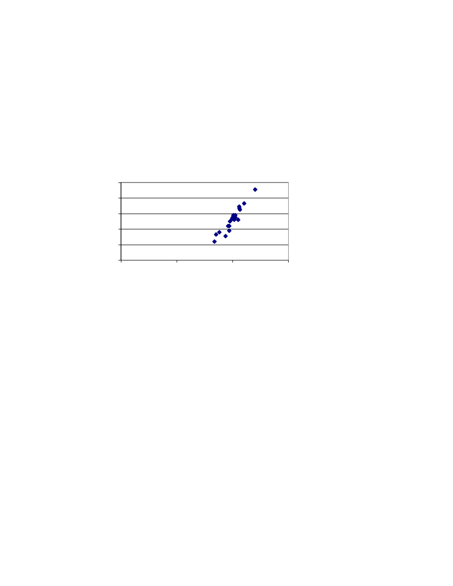
61
Watford 838.3676
Table 3.12 Elo rating parameters after the season 1999-2000.
The parameters in Table 3.12 fairly well describe the final league table. Sheffield
Wednesday seemed to be a better team than their position in the league table
indicates according to the Elo ratings.
Elo ratings vs. Points
0
20
40
60
80
100
0
500
1000
1500
Ratings
Po
in
ts
Figure 3.11 Scatter plot of Elo ratings vs. league points.
The Figure 3.11 shows that there exist a correlation between Elo ratings and the
league points. We make a comparison between Elo and other approaches in
Section 3.5.

62
3.5 Multinomial Ordered Probit Model
The estimates from the probit model for the whole 1999-2000 season data are
provided below:
Team Rating
Manchester U 0.526
Leeds -0.10804
Liverpool -0.12414
Chelsea -0.17516
Aston Villa
-0.32989
Sunderland -0.35387
West Ham
-0.42588
Leicester -0.46225
Everton -0.50042
Newcastle -0.50277
Middlesbrough -0.52043
Tottenham -0.52741
Southampton -0.71523
Coventry -0.73669
Derby -0.84377
Wimbledon -0.92459
Bradford -0.95624
Sheffield W
-1.10025
Watford -1.34273
_cut1 -0.72516
_cut2
0.029611
Table 3.13 Ordered probit rating parameters after the season 1999-2000.
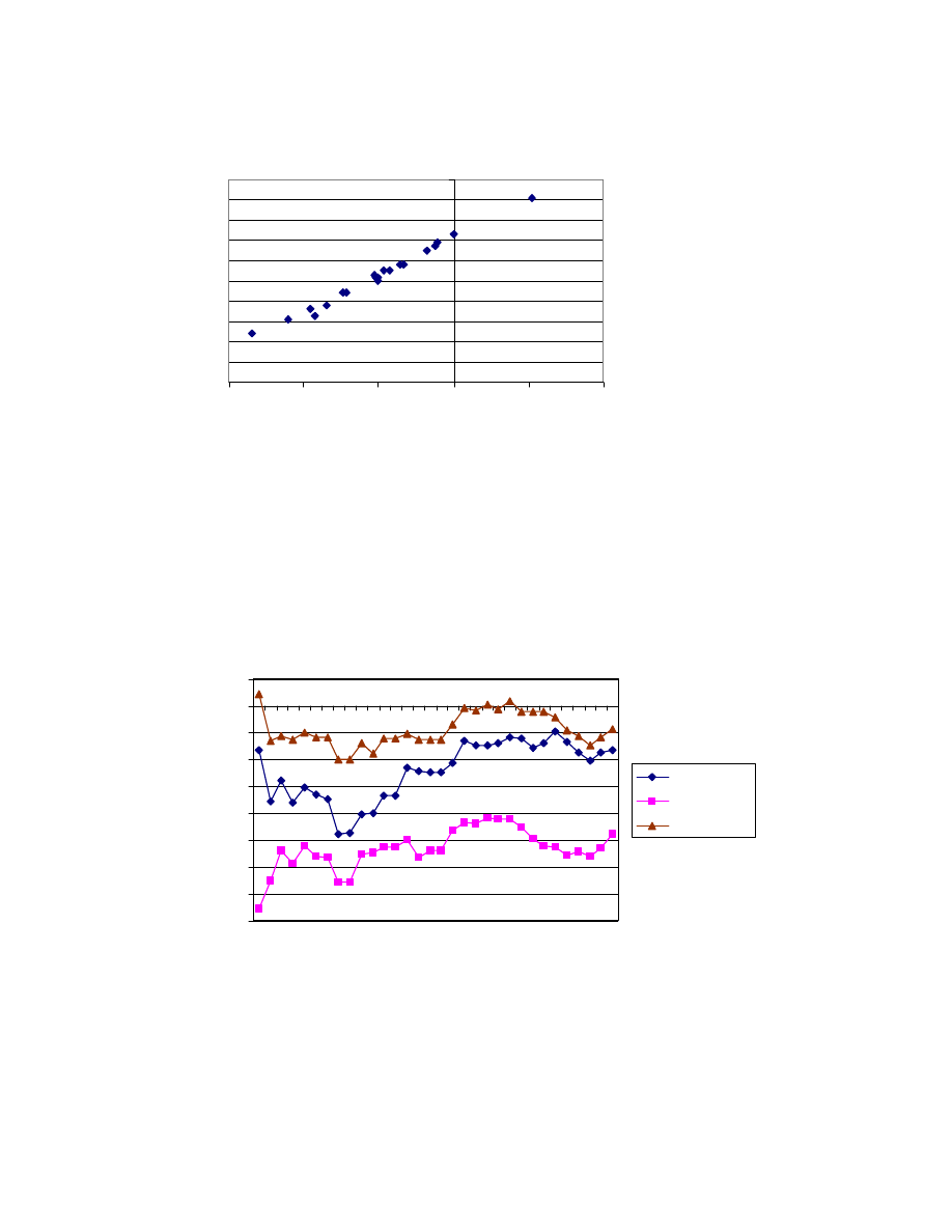
63
Probit vs. Points
0
10
20
30
40
50
60
70
80
90
100
-1.5
-1
-0.5
0
0.5
1
Probit parameters
Po
in
ts
Figure 3.12 Scatter plot of probit parameters vs. league points.
For the whole season data the probit parameters are very consistent with the
league points as seen in the Figure 3.12.
Team strenght
-1.6
-1.4
-1.2
-1
-0.8
-0.6
-0.4
-0.2
0
0.2
14
17
20
23
26
29
32
35
38
41
Time (weeks)
P
a
ra
m
e
ter
esti
m
ate
Aston Villa
Bradford
Chelsea
Figure 3.13 Time series of the maximum likelihood estimates of team strength for Aston Villa,
Bradford and Chelsea.

64
In Figure 3.13, the week-by-week time series chart shows how parameters for
particular teams vary over the season. In the next section, we make a comparison
between probit and other approaches.
3.6 Comparison of Approaches
Next step is to compare the alternative prediction approaches to the best Poisson
regression model (E(Score)&Dep&Weighted in Section 3.3). Elo ratings are
updated week-by-week. Thus, we want to use the week-by-week Poisson and
probit model in comparison. Our point estimate for the comparison is the same as
before, i.e. the sum of the probabilities of the correct outcomes. Now, our
comparison is based on English Premier League 1999-2000 season (November-
May). The table below presents the results obtained by using three different
approaches in prediction:
Model
∑P(correct)
Poisson 102.4316
Probit
105.4185
Elo
96.3732
We notice that probit gives the best estimates and Elo the worst. However, we
use Poisson as it is much more versatile than probit. Probit fits well to fixed odds
betting whereas Poisson can be applied to almost all kinds of betting. That is the
main reason why we establish a betting strategy based on Poisson. Also, the
software for fitting the multinomial ordered probit model was not generally
available.

65
Chapter 4
4 Betting Strategy and Model Validation
4.1 Value Betting
A person who wants make money in sports betting needs to look for odds that
contradict with his/her own probability estimates for a sporting event. This is
strictly mathematical approach to betting. You do not necessarily need to believe
in the team you put your money on. As long as the odds presented are better than
the purely mathematical chance of winning the match, it is a value bet. If you
think that the team has got a 50% chance of winning the match, odds above 2.0
represent the value. If you think the team has only 40% chance, it is no longer a
value bet. Objects with good value are objects, which will give you a positive
payoff over time. The formula for finding an object value is:
r
Percentage
Odds
=
100
*
Eq. 4.1
where r >= 1.0
If the result of the above calculation is a number greater than 1.0, then in theory it
is a value bet. Odds are an inverse of the bookmaker’s estimated probability of an
event to occur. For example, if the odds for a single match are 1.80/3.40/3.50,
then the corresponding probabilities are 0.56, 0.29, 0.29, respectively. These sum
up to 1.14. This is explained by the in-built take that the bookmaker has in order
to run the profitable business as described earlier.

66
The Eq. 4.1 raises the question what threshold should be chosen for r. There is no
direct way to find an optimal value but we investigate that closer in Section 4.4.
4.2 Betting
Strategy
The bookmaker can afford to make slight mistakes and still set odds, which are in
the range that ensure some return. Due to the huge number of matches and events
the bookmakers are dealing with and the volatility of the betting market, it is
impossible for them to avoid mistakes. Some of the mistakes are intentional and
some of them are unintentional.
The intentional mistakes are the ones where the bookmaker is fully aware that the
odds do not reflect to the outcome of the match, but they reflect to the betting
volume. Bookmakers thus take an advantage of punters’ illogical behaviour.
These types of mistakes occur most often in international matches where
patriotism plays a critical role. The effect of mass psychology is also emphasized
in pari-mutuel betting, where the odds are derived based on the bets placed.
The unintentional mistakes are the ones that arise from human errors. The
bookmaker has not taken into account a single factor that has a significant effect
on the outcome of the event, for example motivation, an injury of the key player.
The punters constantly need to look for either one of these mistakes, and when
they find one, they need to place such a stake that will maximize their profit taken
into account the risk attached.
4.3 Money Management
The central problem for a punter is to find a positive expectation bets. But the
punter must also know how much to invest for each betting opportunity. In the
stock market the problem is similar but more complex. The punter, who is now

67
an investor, looks for excess risk adjusted return. In both these settings, the use of
Kelly criterion is worth closer look. It maximizes the expected value of the
logarithm of growth. In Chapter 2, we stated that Kelly criterion was the best
betting strategy to use. We now want to examine how it works in practice.
4.4 Validation on Existing Data
Bookmakers’ odds for the season 2000-2001 were obtained from the web site
oddscomparison.com. After the tenth week of the season, we picked the matches
where r in Eq. 4.1 is greater than 1.1, 1.2, 1.3, 1.4, 1.45, 1.5, 1.6 and 1.7. We also
excluded the last month of the season, because it was found that the model
predictions were poor, possibly due to the end of season effects (motivational).
We want to emphasize that this validation is done week-by-week, and is thus
comparable to the real-life situation. We consider fixed stake, Kelly criterion, ½
Kelly and ¼ Kelly as our money management strategy and see whether our
bankroll ends up with the positive return. The bookmaker we consider is
Centrebet. The company operates in Australia and accepts single bets. The
theoretical return percentage is around 90 %. We focus on the main leagues in
Europe: English Premier League, Division 1, Division 2, Division 3, Italian Serie
A, Spanish Primera Liga and German Bundesliga. Table 4.1 and Figure 4.1 show
how the return percentage varies with different margins and staking strategies.
Margin Fixed% Kelly% 1/2Kelly% 1/4Kelly% #
of
bets
1.1 94.23%
15.95%
61.49%
81.93% 712
1.2 94.44%
34.03%
70.05%
85.26% 346
1.3 96.84%
106.74% 105.02%
96.75% 174
1.4 99.63%
213.85% 156.68% 128.27%
87
1.45 100.53%
248.74% 175.36% 137.88%
72
1.5 101.09%
235.71% 167.97% 134.01%
51
1.6 101.67%
175.13% 137.65% 118.85%
28
1.7 102.07%
170.87% 136.05% 118.15%
23
Table 4.1 Betting statistics with different margins for all leagues in the study.
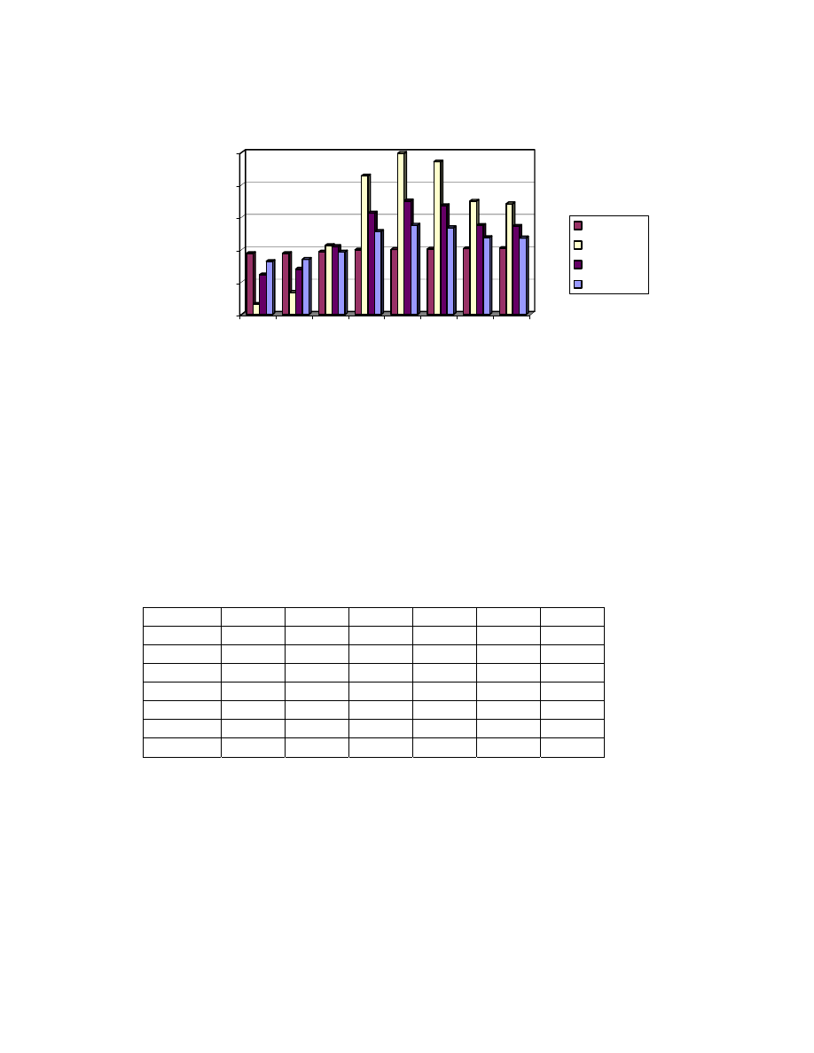
68
0.00%
50.00%
100.00%
150.00%
200.00%
250.00%
1.1
1.2
1.3
1.4
1.45
1.5
1.6
1.7
Margin
Return percentage for all leagues
Fixed%
Kelly%
1/2Kelly%
1/4Kelly%
Figure 4.1 Graphical interpretation of the results for all leagues.
Table 4.1 and Figure 4.1 were constructed for all leagues mentioned earlier. The
optimal margin is at 1.45, and the full Kelly criterion is the most profitable money
management strategy. The last column, the number of bets placed, shows that in
a profitable betting strategy, the value betting opportunities occur quite rarely.
Table 3.2 gives the details of return percentages among different leagues.
Margin Fixed% Kelly%
1/2Kelly%1/4Kelly% #
of
bets
Premier
1.45 116.35% 517.51% 308.76% 204.38%
10
Division1
1.45 115.10% 994.51% 547.26% 323.63%
9
Division2
1.45 96.35% 28.05% 64.03% 82.01% 11
Division3
1.45 100.50%
58.70% 79.35% 89.67%
6
BundesLiga
1.45 99.75%
132.87% 116.44% 108.22%
5
SerieA
1.45 88.75% 4.84% 52.42%
76.21% 18
PrimeraLiga
1.45 86.90% 4.69% 59.29%
81.03% 13
Table 4.2 Betting statistics among different leagues.
We notice that English Premier League and Division One would have given the
best returns, whereas betting on Italian Serie A and Spanish Primera Liga we
would have lost money. The number of bets seems relatively large in Italian Serie
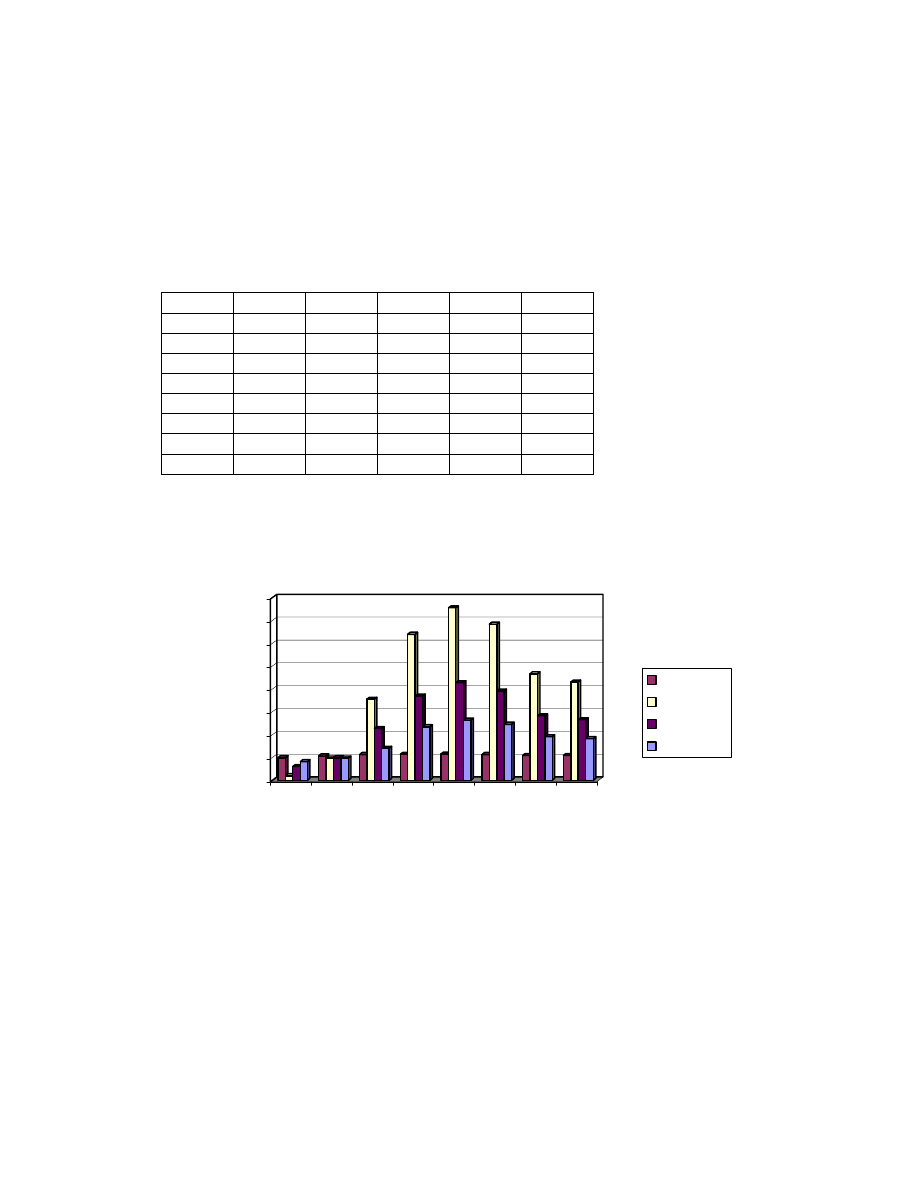
69
A compared to other leagues. Italian football has a very defence oriented
tradition, and the Poisson approach might not be as suitable for Serie A’s low
scoring matches. Because English Premier League and Division One gave us
significantly highest returns, we want to investigate these two leagues more
closely in Table 4.3 and Figure 4.2.
Margin Fixed% Kelly%
1/2Kelly%1/4Kelly% #
of
bets
1.1
99.21% 20.81% 60.40% 82.32% 217
1.2
107.15% 98.38% 99.19% 98.28% 95
1.3
113.38% 355.15% 227.58% 141.41%
49
1.4
114.48% 639.70% 369.85% 234.92%
24
1.45
115.73% 756.01% 428.01% 264.00%
19
1.5
113.68% 684.19% 392.09% 246.05%
15
1.6
109.58% 466.35% 283.18% 191.59%
9
1.7
109.50% 431.47% 265.74% 182.87%
7
Table 4.3 Betting statistics with different margins for English Premier League and Division 1.
0.00%
100.00%
200.00%
300.00%
400.00%
500.00%
600.00%
700.00%
800.00%
1.1
1.2
1.3
1.4
1.45
1.5
1.6
1.7
Margin
Return chart for Prem and Div 1
Fixed%
Kelly%
1/2Kelly%
1/4Kelly%
Figure 4.2 Graphical interpretation of the results for English Premier League and Division 1.
These above charts agree that the best margin is found at the value 1.45. We
could investigate the optimal time varying value of the margin in a more
sophisticated manner than trial and error, but we leave it for further work.

70
The results of this betting simulation are fairly encouraging considering the fact
that the return percentages at their best climbed as high as 750 %. Variation in
the return percentages among different leagues is noticeable and needs further
analysis. However, the idea of earning significant profits based on this betting
strategy is very interesting.

71
Chapter 5
5 Discussion
5.1 Implementation of the System
During the research, we were forced to automate the whole process in order to
minimize the time spent in results/odds updating. Initially the data was just
copied and pasted between Excel and S-Plus, but as I got more into writing Visual
Basic macros, it enabled us to leave out all the unnecessary tasks and improved
the efficiency tremendously. Of course, we could have done everything in S-Plus,
but because the data manipulation is currently user-friendlier in Excel, we decided
to apply both of these programs. Also, retrieving external data by web queries
was very handy in Excel. However, by learning to manipulate data effectively in
a matrix form makes S-Plus probably superior to Excel. Figure 5.1 describes the
final automation process. Personally, I want to emphasize that the customization
was non-trivial and it was an integral part of the success of the project. Learning
how to make custom solutions with MS Office components and interacting with
various applications was one of the most rewarding experiences of this project.
The Visual Basic code is not included in the Appendix because of the potential
market value it may contain.
72
Data Flow
Figure 5.1 Implementation data flow of the components involved.
Data storing component is optional and we only used Excel for that. For
professional punting, though, it would be very important to keep track on one’s
progress and without proper data storing it is not possible. It is also necessary in
further development of the system.
5.2 Applications of the System
The system has several applications both from bookmaker’s and punter’s point of
views. We take a closer look at both of these in the following.
Access
Data storing
Excel
Data output
S-Plus
Data analysis
Excel
Data filtering
Results
http://sunsite.tut.fi/rec/riku/soccer.html
Odds
http://www.oddscomparison.com

73
5.2.1 Bookmaker’s Point of View
The risk management will play more and more crucial role, as the sports betting
becomes more interactive and the competition accelerates. Better tools need to be
developed in order to avoid setbacks in the market. Even though, the sports
betting industry has tremendously increased in recent years, still quite a few
bookmakers are applying rather non-scientific methods in determining the odds
for various sporting events.
In order to set the betting distribution evenly, it is not all about predicting the
outcome. For example, a common habit among the punters is to play the superior
team. Teams, such as Manchester United, receive very low odds because punters
want to win as often as possible. It is vital to take these factors into account when
determining the final price.
A statistically proper system that predicts probabilities with reasonable accuracy
and also monitors the betting distribution is a vital tool for them as more and more
matches need to be covered and more attractive prices need to be compiled. The
system would immediately notice if the distribution is unbalanced, and the odds
do not reflect the punters' opinion. It would also warn the operator of possible
risky situation involving professional punters.
As a result of this, the bookmaker can offer more accurate odds, which allows
them to increase the theoretical return percentage to the punters and thus be more
competitive in the market.
5.2.2 Punter’s Point of View
Some people consider betting systems as a well-organized way to lose money.
Others believe there is a system that will ultimately make their dreams come true.
The basic principle in profitable betting is that you can only win in the long run

74
by consistently trading when the odds are on your side. There are several things
that need to be considered, though. Doing the research does not need to make
sports betting boring. In fact, when the result goes your way, it makes it even
more satisfying. Conversely, the result that defies logic and goes against all your
reasoning may be infuriating, but it may also teach you where you are doing
something wrong and sharpen your technique.
The vast majority of punters has always, and will always lose money. What is
needed the most is the confidence to back one’s own judgment ahead of everyone
else’s. The punters can take an advantage of bookmakers’ inadequate risk
management. In this study, we have validated that opportunities for profitable
betting exist and created a system, which monitors and notifies the user if the
odds for an event determined by the bookmaker do not reflect the true odds for
that particular event. With this system we demonstrated that the return could lead
up to 650 % profit.

75
Chapter 6
6 Summary and Future Work
6.1 Summary
The models we have proposed here have proven to be useful in the gaming
market. We investigated the benefits of using the Poisson model from
bookmaker’s and punter’s point of views and concluded that it would have
potential to improve both of their performance. During the upcoming years when
majority of government licensed sports books make their transition from online
terminals into the Internet, the competition will increase. Also, the dilemma of
government licensed sports books vs. offshore sports books will bring more
emphasis on risk management in the gaming business. According to market
research studies, the sports betting will have an increasing entertainment value
among people with the penetration of new technology. Punters are interested in
the system that would increase their return on investment and operators on the
other hand need to pay closer attention on risk management. Thus, a tool that is
capable of doing that must have a market value.
6.2 Future Work
Many things could be considered in the search of getting more accurate
probability estimates for sporting events. The main thing is to determine which
ones are really worth closer numerical analysis. Injuries, suspensions and weather
conditions certainly have an effect on the outcome of the match. We consider few
possible improvements of the model in the following.

76
6.2.1 Residual Correction
One thing that we have not discussed in the thesis is residual correction. In Jay
Bennett’s book Statistics in Sport (1998), Pjotr Janmaat implemented exponential
smoothing factor into Maher’s original model
k
i
k
j
k
j
k
i
k
i
ad
aa
ad
ha
z
*
*
1
−
=
+
Eq. 6.1
To update ha, for example,
)
*
)
2
/
(
1
(
*
1
k
k
i
k
i
correction
factor
ha
ha
+
=
−
Eq. 6.2
The correction in Eq. 6.2 equals predicted minus actual home goals divided by
predicted home goals. A similar equation updates the other parameters. The
home team’s home parameters and away team’s away parameters are adjusted
using an average factor 0.16. The home team’s away parameters and the away
team’s home parameters are adjusted with an average factor 0.055, selected
empirically. This correction method sounds a little ad hoc and we leave it for
further work.
6.2.2 Other Types of Betting
So far we have mostly focused on fixed odds betting. Poisson model is also very
interesting in Asian handicap and spread betting, because it predicts the expected
number of goals scored by both teams. In Table 5.1 we see the output of the
Excel worksheet, which can be applied to Asian Handicap betting.

77
Date Home
Away
H
A
Asian
Hcap
OddsH
OddsA
14/4/2001 West Ham
Derby
3
1
-1 ¼
2.064 1.939
14/4/2001 Sunderland
Tottenham
2
3
-
½
2.058 1.945
14/4/2001 Manchester U
Coventry
4
2
-1 ¾
1.389 3.570
14/4/2001 Leicester
Manchester C
1
2
-1
2.071 1.933
14/4/2001 Ipswich
Newcastle
1
0
-
¾
2.058 1.944
14/4/2001 Chelsea
Southampton
1
0
-1
¼
2.012 1.988
14/4/2001 Aston Villa
Everton
2
1
- ¾
1.905 2.104
14/4/2001 Arsenal
Middlesbrough
0
3
-1
2.081 1.924
13/4/2001 Liverpool
Leeds
1
2
-1
¼
2.080 1.925
13/4/2001 Bradford
Charlton
2
0
¼
1.798 2.251
11/4/2001 Manchester C
Arsenal
0
4
¾
1.564 2.771
10/4/2001 Tottenham
Bradford
2
1
-1
¼
1.949 2.053
10/4/2001 Manchester U
Charlton
2
1
-1 ¾
1.487 3.052
10/4/2001 Ipswich
Liverpool
1
1
¼
1.980 2.01
9/4/2001
Middlesbrough
Sunderland 0
0 -
¼
2.011
1.988
8/4/2001
Everton
Manchester C
3
1
- ¾
1.974 2.025
7/4/2001
Aston Villa
West Ham
2
2
- ¾
2.113 1.898
7/4/2001 Leicester
Coventry
1 3
-1
¼
2.092 1.914
7/4/2001
Leeds
Southampton
2
0
-1
1.968 2.032
7/4/2001 Derby
Chelsea
0 4
¾
1.568 2.758
4/4/2001
Aston Villa
Leicester
2
1
- ½
1.940 2.063
2/4/2001 Southampton Ipswich
0 3
-
¼
2.065 1.938
1/4/2001 Charlton
Leicester
2 0
-
¼
2.126 1.887
Table 5.1 The Excel output of the Asian Handicap probabilities based on the model.
Here H = home goals and A = away goals. The Asian Handicap (Asian Hcap),
and the odds with the handicap (OddsH, OddsA) were obtained based on the
model with implemented program described in Section 5.1. We were not able to
collect Asian Handicap odds in order to compare those to our model estimates.
With the above we just want to demonstrate the versatility of Poisson model in
different types of betting. In Table 5.2 we see the similar output of the Excel
worksheet, which can be applied to spread betting.

78
Date Home
Away
H
A
E(H)
E(A)
E(BH)
E(BA)
14/4/2001
West
Ham
Derby
3 1 1.907 0.737 1.363 0.852
14/4/2001
Sunderland Tottenham
2 3 1.370 0.932 1.405 0.787
14/4/2001
Manchester
U Coventry
4 2 3.706 0.503 1.961 0.489
14/4/2001
Leicester
Manchester
C 1 2 1.774 0.859 1.455 0.827
14/4/2001
Ipswich
Newcastle
1 0 1.644 0.962 1.525 0.785
14/4/2001
Chelsea
Southampton
1 0 2.119 0.885 1.666 0.558
14/4/2001
Aston
Villa Everton
2 1 1.620 0.755 1.424 0.858
14/4/2001
Arsenal
Middlesbrough 0 3 1.563 0.655 1.867 0.640
13/4/2001
Liverpool
Leeds
1 2 1.965 0.816 1.349 1.032
13/4/2001
Bradford
Charlton
2 0 0.991 1.312 1.171 1.262
11/4/2001
Manchester
C Arsenal
0 4 0.884 1.714 0.858 1.424
10/4/2001
Tottenham Bradford
2 1 1.998 0.681 1.679 0.637
10/4/2001
Manchester
U Charlton
2 1 3.248 0.433 1.966 0.663
10/4/2001
Ipswich
Liverpool
1 1 1.357 1.336 1.107 1.066
9/4/2001 Middlesbrough
Sunderland
0 0 1.002 0.763 1.206 1.177
8/4/2001 Everton
Manchester
C 3 1 1.755 0.974 1.392 0.821
7/4/2001
Aston Villa
West Ham
2
2
1.419
0.790
1.397
0.769
7/4/2001 Leicester
Coventry
1 3 1.688 0.546 1.528 0.914
7/4/2001 Leeds
Southampton
2 0 2.019 0.978 1.507 0.569
7/4/2001 Derby
Chelsea
0 4 0.976 1.772 1.148 1.162
4/4/2001 Aston
Villa Leicester
2 1 1.254 0.690 1.322 0.852
2/4/2001 Southampton Ipswich
0 3 1.199 1.015 1.272 1.058
1/4/2001 Charlton
Leicester
2 0 1.160 1.034 1.320 0.997
Table 5.2 The Excel output of the model E(Score) vs. bookmaker E(Score).
Here H = home goals and A = away goals. E(H) and E(A) are predicted goals
from the model. E(BH) and E(BA) are Centrebet’s expected number of home and
away goals derived based on the Poisson assumption. The above output could be
applied to the Total Goals and the Supremacy bets in the spread betting market.
For example, in Total Goals betting our point estimate in the match West Ham-
Derby is E(West Ham)+E(Derby) = 1.907 + 0.737 = 2.644. If the spread betting
company would offer the spread 1.9 - 2.1 we would definitely consider this as a
value bet opportunity.
This is another example of the versatility of the Poisson model. We leave the
analysis of profitable betting in Asian Handicap and spread betting for further
work.

79
6.2.3 Bayesian Framework
Due to the fluctuation in the leagues, sometimes there is not enough data for the
classical frequentist approach. Similar setting arises in cup matches and
international tournaments. Therefore, the use of various simulation methods could
be beneficial in these types of occasions. The prior information for simulation
could be obtained from the expert opinions.
At least two articles are written where Bayesian approach is incorporated into the
model to predict result in sporting events. One was done by Håvard Rue and
Öyvind Salvesen where they applied a Bayesian dynamic generalized linear
model in order to predict next weekend’s football matches. They applied Markov
Chain Monte Carlo (MCMC) technique to generate dependent samples from the
posterior density. They also applied Brownian motion to take into account the
time varying properties of attack and defence parameters. A similar study was
conducted for American football by Glickman and Stern (1998). We do not
consider Baysian approach in terms of this thesis any further, but foresee it as an
interesting topic for future work.

80
Appendices
Appendix A
Odds Dividend % Odds Dividend % Odds Dividend %
1/10
1.10 91
16/10
2.60 38
12/1
13.00 8
1/8
1.13 89
18/10
2.80 36
14/1
15.00 7
1/7
1.14 88
2/1
3.00 33
15/1
16.00 6
1/6
1.17 86
22/10
3.20 31
16/1
17.00 6
1/5
1.20 83
25/10
3.50 29
20/1
21.00 5
1/4
1.25 80
28/10
3.80 26
25/1
26.00 4
2/7
1.29 78
3/1
4.00 25
30/1
31.00 3
1/3
1.33 75
32/10
4.20 24
33/1
34.00 3
4/10
1.40 71
35/10
4.50 22
40/1
41.00 2
4/9
1.45 69
4/1
5.00 20
50/1
51.00 2
1/2
1.50 67
45/10
5.50 18
60/1
61.00 2
6/10
1.60 63
5/1
6.00 17
80/1
81.00 1
7/10
1.70 59
55/10
6.50 15
100/1
101.00
1
8/10
1.80 56
6/1
7.00 14
150/1
151.00
1
9/10
1.90 53
65/10
7.50 13
200/1
201.00
-
EVEN
2.00 50
7/1
8.00 12
250/1
251.00
-
11/10
2.10 48
8/1
9.00 11
300/1
301.00
-
12/10 2.20
46 9/1
10.00
10 400/1 401.00 -
14/10 2.40
42 10/1 11.00 9 500/1 501.00 -
15/10 2.50
40 11/1 12.00 8 -
-
-

81
Appendix B
Result calculation:
The table shows the winning/losing percentages. "No bet" means
that the stake will be refunded.
-
Handicaps
Result
0 : 0
1 : 0
0 : 1
2 : 0
3 : 0
Home
Away
0
0
-
no bets
+100%
-100%
-100%
+100%
+100%
-100%
+100%
-100%
Home
Away
0
¼
-
-50%
+50%
+100%
-100%
-100%
+100%
+100%
-100%
+100%
-100%
Home
Away
0
½
-
-100%
+100%
+100%
-100%
-100%
+100%
+100%
-100%
+100%
-100%
Home
Away
0
¾
-
-100%
+100%
+50%
-50%
-100%
+100%
+100%
-100%
+100%
-100%
Home
Away
0
1
-
-100%
+100%
no bets
-100%
+100%
+100%
-100%
+100%
-100%
-
Handicaps
Result
0 : 0
1 : 0
0 : 1
2 : 0
3 : 0
Home
Away
0
1¼
-
-100%
+100%
-50%
+50%
-100%
+100%
+100%
-100%
+100%
-100%
Home
Away
0
1½
-
-100%
+100%
-100%
+100%
-100%
+100%
+100%
-100%
+100%
-100%
Home
Away
0
1¾
-
-100%
+100%
-100%
+100%
-100%
+100%
+50%
-50%
+100%
-100%
Home
Away
0
2
-
-100%
+100%
-100%
+100%
-100%
+100%
no bets
+100%
-100%
Home
Away
0
2¼
-
-100%
+100%
-100%
+100%
-100%
+100%
-50%
+50%
+100%
-100%

82
Appendix C
Final
bankroll
Number of seasons final bankroll was:
(starting with $1000)
System
Min. Max. Mean Median Bankrupt >$2 >$250 >$500 >$1000 >$5000 >$10000 >$50000 >$100000
Kelly
18 453883 48135 17269 0
1000 957 916 870
692
598
302
166
½Kelly
145 111770 13069 8043
0
1000 999 990 954
654
430
430
1
Fixed:
$10
307
3067
1861
1857
0 1000
1000
999
980
0 0 0 0
$20
0 5377 2824 2822 9
991 990 988 978 9
0
0
0
$30
0 7682 3739 3770 36
964 963 962 957 191
0
0
0
$40
0 9986 4495 4685 94
906 906 906 904 432
0
0
0
$50
0 12282 5213 5526 134
866 866 866 864 584
33
0
0
$100
0 23747 7637 8722 349
651 651 651 651 613
425
0
0
Proportional:
1%
435
8469
2535
2270
0 1000
1000
999
965
43
0 0 0
2%
173 57087
6628
4360 0
1000
999 991 940 443 180 7
0
3%
65 243281 15343 6799
0
1000 994 973 919
592
396
65
18
4%
49 483355 26202 8669
0
1000 979 935 882
627
459
146
61
5%
38 548382 32415 8970
0
1000 941 899 841
609
475
179
90
10%
18 364587 13662 602
0
1000 575 515 455
304
221
78
36

83
Appendix D
*** Generalized Linear Model ***
Coefficients:
Arsenal.att=0 to avoid overparametrisation
Value Std. Error t value
arsenal.home 0.303682385 0.2367505 1.28271046
aston.villa.home -0.303683460 0.3780379 -0.80331481
bradford.home 0.469465669 0.4207814 1.11569964
chelsea.home 0.361293961 0.3743586 0.96510126
coventry.home 1.136661472 0.4390941 2.58865142
derby.home -0.303680108 0.3830637 -0.79276659
everton.home 0.144342465 0.3567045 0.40465553
leeds.home -0.303683211 0.3534958 -0.85908584
leicester.home -0.047749061 0.3604239 -0.13248028
liverpool.home -0.106971918 0.3676345 -0.29097355
manchester.u.home 0.136268883 0.3151321 0.43241830
middlesbrough.home -0.303681944 0.3780597 -0.80326449
newcastle.home 0.389464858 0.3569886 1.09097290
sheffield.w.home -0.092370516 0.4022720 -0.22962204
southampton.home 0.009974913 0.3835162 0.02600911
sunderland.home -0.338773846 0.3552650 -0.95358079
tottenham.home 0.551983856 0.3739691 1.47601443
watford.home 0.476465849 0.4338279 1.09828297
west.ham.home 0.166320249 0.3703943 0.44903562
wimbledon.home 0.324924580 0.3895620 0.83407661
aston.villa.att -0.307432011 0.2751960 -1.11713857
bradford.att -0.925918991 0.3390112 -2.73123456
chelsea.att -0.553300637 0.2964089 -1.86668030
coventry.att -1.227002906 0.3778787 -3.24708171
derby.att -0.330389324 0.2787667 -1.18518222
everton.att -0.293117357 0.2752777 -1.06480601
leeds.att -0.067333337 0.2583983 -0.26057961
leicester.att -0.244762537 0.2719770 -0.89993829
liverpool.att -0.312132419 0.2752296 -1.13408009
manchester.u.att 0.206745180 0.2421754 0.85370023
middlebrough.att -0.290782718 0.2753015 -1.05623350
newcastle.att -0.378860369 0.2827372 -1.33997348
sheffield.w.att -0.575640089 0.3013701 -1.91007727
southampton.att -0.471961467 0.2914442 -1.61938857
sunderland.att -0.054406128 0.2584713 -0.21049191
tottenham.att -0.595496064 0.3019179 -1.97237779
watford.att -1.004180511 0.3505182 -2.86484523
west.ham.att -0.429241927 0.2868111 -1.49660175
wimbledon.att -0.631678163 0.3078130 -2.05214902
arsenal.def 0.292153466 0.2377898 1.22862063
aston.villa.def 0.059135710 0.2446323 0.24173307
bradford.def 0.716762700 0.2145240 3.34117754
chelsea.def 0.036921825 0.2462058 0.14996327
coventry.def 0.494600377 0.2232096 2.21585596
derby.def 0.545827013 0.2210070 2.46972673
everton.def 0.409121810 0.2273277 1.79970067
leeds.def 0.277158663 0.2335210 1.18686819
leicester.def 0.520972855 0.2224359 2.34212543
liverpool.def -0.090390870 0.2541715 -0.35562951
manchester.u.def 0.362341831 0.2311703 1.56742413
middlesbrough.def 0.455779801 0.2247700 2.02776098

84
newcastle.def 0.510609088 0.2231491 2.28819703
sheffield.w.def 0.745825778 0.2135447 3.49259868
southampton.def 0.631124530 0.2177828 2.89795335
sunderland.def 0.541054222 0.2216942 2.44054291
tottenham.def 0.407124183 0.2273721 1.79056342
watford.def 0.838388265 0.2104918 3.98299648
west.ham.def 0.480830355 0.2239260 2.14727349
wimbledon.def 0.809610232 0.2117130 3.82409300
(Dispersion Parameter for Poisson family taken to be 1 )
Null Deviance: 1088.126 on 760 degrees of freedom
Residual Deviance: 791.8831 on 701 degrees of freedom
Table D.1 S-Plus output of the Poisson regression with separate home parameters for season
1999-2000.
*** Generalized Linear Model ***
Coefficients:
Arsenal.att=0 to avoid overparametrisation
Value Std. Error t value
home 0.41150035 0.08998748 4.57286224
aston.villa.att -0.65778773 0.29045847 -2.26465325
bradford.att -0.79387805 0.30871345 -2.57156938
chelsea.att -0.22153164 0.26881944 -0.82409084
coventry.att -0.27469639 0.25879297 -1.06145228
derby.att -0.69117432 0.30250397 -2.28484376
everton.att -0.01129526 0.24368842 -0.04635125
leeds.att -0.07030137 0.24070688 -0.29206215
leicester.att -0.24039328 0.25439950 -0.94494398
liverpool.att -0.18878526 0.24731103 -0.76335156
manchester.u.att 0.36718582 0.22259721 1.64955268
middlesbrough.att -0.39130379 0.26880272 -1.45572854
newcastle.att -0.06278067 0.24508225 -0.25616165
sheffield.w.att -0.64285630 0.30053369 -2.13904906
southampton.att -0.37133632 0.27714141 -1.33988031
sunderland.att -0.01324357 0.24372629 -0.05433788
tottenham.att -0.09083232 0.24936785 -0.36425033
watford.att -0.83996814 0.31708890 -2.64899888
west.ham.att -0.36066921 0.27758533 -1.2993093
wimbledon.att -0.12965245 0.24688175 -0.52516012
arsenal.def 0.04836594 0.28964110 0.16698575
aston.villa.def 0.01452591 0.28439652 0.05107626
bradford.def 0.40401393 0.25396720 1.59081144
chelsea.def 0.04657717 0.29425112 0.15829056
coventry.def 0.16913505 0.27674268 0.61116360
derby.def 0.44892437 0.24260982 1.85039654
everton.def 0.33024934 0.25667292 1.28665439
leeds.def 0.10687328 0.27557032 0.38782582
leicester.def 0.34976641 0.25058493 1.39579988
liverpool.def -0.09360267 0.29939517 -0.31263922
manchester.u.def 0.30612137 0.27015372 1.13313772
middlesbrough.def 0.40477409 0.25992061 1.55729894
newcastle.def 0.56025126 0.24346025 2.30120223
sheffield.w.def 0.82196321 0.24305033 3.38186418
southampton.def 0.41094196 0.25725478 1.59741234

85
sunderland.def 0.26128400 0.27698961 0.94329892
tottenham.def 0.22564444 0.27646742 0.81617009
watford.def 0.66935126 0.23598115 2.83646069
west.ham.def 0.07217156 0.28596980 0.25237477
wimbledon.def 0.60385220 0.24273300 2.48772190
(Dispersion Parameter for Poisson family taken to be 1 )
Null Deviance: 549.8061 on 760 degrees of freedom
Residual Deviance: 392.8681 on 340 degrees of freedom
Table D.2 S-Plus output of the first half of the season 99-00
*** Generalized Linear Model ***
Coefficients:
Arsenal.att=0 to avoid overparametrisation
Value Std. Error t value
home 0.37463060 0.08901497 4.20862491
aston.villa.att -0.39163024 0.25260782 -1.55034887
bradford.att -0.54272934 0.26726749 -2.03065981
chelsea.att -0.42374071 0.24732011 -1.71332897
coventry.att -0.59704330 0.27456666 -2.17449307
derby.att -0.40038806 0.25173327 -1.59052501
everton.att -0.43686698 0.25838984 -1.69072815
leeds.att -0.43828573 0.26384727 -1.66113421
leicester.att -0.31540003 0.25447143 -1.23943202
liverpool.att -0.62770692 0.27949432 -2.24586645
manchester.u.att 0.15962732 0.21985332 0.72606284
middlesbrough.att -0.49402055 0.26779904 -1.84474357
newcastle.att -0.27331082 0.24571065 -1.11232797
sheffield.w.att -0.66525973 0.27128318 -2.45227045
southampton.att -0.62185816 0.26470579 -2.34924276
sunderland.att -0.52184578 0.26465258 -1.97181443
tottenham.att -0.39213443 0.25521010 -1.53651615
watford.att -0.61129731 0.27593916 -2.21533368
west.ham.att -0.33900559 0.24635067 -1.37610989
wimbledon.att -0.87753010 0.30771276 -2.85178325
arsenal.def 0.47384249 0.27645732 1.71398059
aston.villa.def 0.01110346 0.30759285 0.03609793
bradford.def 0.94445940 0.23158170 4.07829883
chelsea.def -0.06217843 0.30020306 -0.20712124
coventry.def 0.68983187 0.24339570 2.83419907
derby.def 0.53144334 0.26693576 1.99090351
everton.def 0.43041210 0.27436636 1.56874950
leeds.def 0.36067882 0.27543666 1.30948010
leicester.def 0.63611025 0.26339929 2.41500362
liverpool.def -0.16140012 0.32284384 -0.49993248
manchester.u.def 0.34324080 0.27249198 1.25963633
middlesbrough.def 0.45891930 0.25947522 1.76864403
newcastle.def 0.30853180 0.28299832 1.09022484
sheffield.w.def 0.53196442 0.24280234 2.19093613
southampton.def 0.70255013 0.24001490 2.92711041
sunderland.def 0.74674898 0.23887203 3.12614660
tottenham.def 0.51161880 0.25485368 2.00750016
watford.def 0.86981002 0.23485594 3.70358959

86
west.ham.def 0.70957649 0.23983304 2.95862691
wimbledon.def 0.96889237 0.23164408 4.18267701
(Dispersion Parameter for Poisson family taken to be 1 )
Null Deviance: 538.3198 on 760 degrees of freedom
Residual Deviance: 393.6574 on 340 degrees of freedom
Table D.3 S-Plus output of the second half of the season 99-00
*** Generalized Linear Model ***
Coefficients:
Arsenal.att=0 to avoid overparametrisation
Value Std. Error t value
home 0.40591095 0.07282501 5.5737846
aston.villa.att -0.47979004 0.21538092 -2.2276348
bradford.att -0.61259129 0.22647018 -2.7049535
chelsea.att -0.39557812 0.20826794 -1.8993712
coventry.att -0.48764476 0.21856073 -2.2311637
derby.att -0.49088847 0.21761700 -2.2557450
everton.att -0.28784336 0.20422998 -1.4094079
leeds.att -0.31753413 0.20617113 -1.5401483
leicester.att -0.33077135 0.20745252 -1.5944436
liverpool.att -0.43400706 0.21192459 -2.0479316
manchester.u.att 0.25839786 0.17814668 1.4504781
middlesbrough.att -0.49183787 0.21753190 -2.2609919
newcastle.att -0.20214264 0.19972964 -1.0120813
sheffield.w.att -0.61964978 0.22689188 -2.7310355
southampton.att -0.56379807 0.22130976 -2.5475518
sunderland.att -0.31237692 0.20685824 -1.5101014
tottenham.att -0.30513754 0.20514902 -1.4873946
watford.att -0.70207625 0.23503549 -2.9871074
west.ham.att -0.35833228 0.20716221 -1.7297184
wimbledon.att -0.54843871 0.22430948 -2.4450090
arsenal.def 0.32821245 0.22712931 1.4450467
aston.villa.def 0.03356866 0.24192702 0.1387553
bradford.def 0.74276967 0.19462746 3.8163663
chelsea.def 0.02961975 0.23806707 0.1244177
coventry.def 0.52904905 0.20471127 2.5843669
derby.def 0.51412536 0.20863993 2.4641753
everton.def 0.37150090 0.21728363 1.7097510
leeds.def 0.25820618 0.22288523 1.1584715
leicester.def 0.52439399 0.20897603 2.5093499
liverpool.def -0.14734253 0.25574469 -0.5761313
manchester.u.def 0.33439608 0.22270048 1.5015507
middlesbrough.def 0.41159291 0.21142015 1.9468008
newcastle.def 0.39197088 0.21559141 1.8181192
sheffield.w.def 0.66972079 0.19628842 3.4119222
southampton.def 0.60312655 0.20113400 2.9986306
sunderland.def 0.58115407 0.20421914 2.8457375
tottenham.def 0.39913306 0.21308129 1.8731492
watford.def 0.85381420 0.18921067 4.5125055
west.ham.def 0.52873345 0.20420958 2.5891707
wimbledon.def 0.80526325 0.19030534 4.2314276

87
(Dispersion Parameter for Poisson family taken to be 1 )
Null Deviance: 807.0231 on 760 degrees of freedom
Residual Deviance: 605.9874 on 720 degrees of freedom
Table D.4 S-Plus output of the weighted model

88
References
Anderson J.A. (1984), Regression and Ordered Categorical Variables, Journal of
Royal Statistical Society, Vol. 46, 1-30.
Bennett J. (1998), Statistics in Sport, Arnold.
Bradley R. A. and Terry M. E. (1952), Rank Analysis of Incomplete Block
Designs. I. The Method of Paired Comparisons, Biometrika, Vol. 39, 324-345.
Burke A. (1998), Spread Betting, Rowton Press.
Clarke S. R. and Norman J. M. (1995), Home Ground Advantage of Individual
Clubs in English Soccer, The Statistician, Vol. 4, 509-521.
Datamonitor (1999), Online Games and Gambling in Europe and the US 1999-
2004.
Dixon M. J. and Coles S. G. (1997), Modelling Association Football Scores and
Inefficiences in the Football Betting Market, Applied Statistics, Vol. 46, 265-280.
Dixon M. J. and Robinson M. E. (1998), A Birth Process Model for Association
Football Matches, The Statistician, Vol. 47, 523-538.
Dobson A. J. (1990), An Introduction to Generalized Linear Models, Chapman &
Hall.
Elo A. E. (1978), The Rating of Chess Players Past and Present, Batsford.

89
Ernst & Young (2000), Winners and Losers – The Future of Online Betting.
Fahrmeir L. and Tutz G. (1994), Dynamic Stochastic Models for Time-Dependent
Ordered Paired Comparison Systems, Journal of American Statistical Association,
Vol. 89, 1438-1449.
Forrest D. and Simmons R. (2000), Work of Football Pools Panel, The
Statistician, Vol. 49, 253-260.
Glickman M. E. and Stern H. S. (1998), A State-Space Model for National
Football League Scores, Journal of American Statistical Association, Vol. 93, 25-
35.
Glickman M.E. and Jones A. C.(1999), Rating the Chess Rating System, Vol.12,
21-28.
Harvey G. (1998), Successful Spread Betting, Take That Ltd.
Harville D. (1980), Predictions for National Football League Games via Linear-
Model Methodology, Journal of American Statistical Association, Vol. 75, 516-
524.
Hausch D. B., Lo V. S. Y. and Ziemba W. T. (1994), Efficiency of Racetrack
Betting Markets, Academic Press.
Hill I. D. (1974), Association Football and Statistical Inference, Applied
Statistics, Vol. 23, 203-208.
Jackson D. A. (1994), Index Betting on Sports, Statistician, Vol. 43, 309-315.
Jacobs S. (1999), Optimal Betting,

90
<URL:www.bjmath.com/bjmath/Betsize/sjopt.html>.
Jones A. (1996), College Soccer Ratings,
<URL:www.reed.edu/~jones/ratings/node1.html>.
Kelly J. L. Jr. (1956), A New Interpretation of Information Rate, The Bell System
Technical Journal, 917-926.
Lee A. J. (1997), Modeling Scores in the Premier League: Is Manchester United
Really the Best?, Chance, Vol. 10, 15-19.
Maher M. J. (1982), Modelling Association Football Scores, Statistica
Neerlandica, Vol. 36, 109-118.
McCullach P. and Nelder J. A. (1983), Generalized Linear Models, Chapman &
Hall.
McCullach P. (1980), Regression Models for Ordinal Data, Journal of Royal
Statistical Society, Vol. 42, 109.142.
River City Group (2000), Wagering on the Internet.
Rue H. and Salvesen Ø. (2000), Prediction and Retrospective Analysis of Soccer
Matches in a League, The Statistician, Vol. 49, 399-418.
Stefani R. T. (1980), Improved Least Squares Football, Basketball and Soccer
Predictions, IEEE transactions on systems, man, and cybernetics, Vol. SMC-10,
116-123.
Stern H. (1999), The Man Who Makes the Odds: An Interview with “Roxy”
Roxborough, Chance, Vol.12, 15-21.

91
Thorp E. O. (1997), The Kelly Criterion in Blackjack, Sports Betting, and the
Stock Market, The 10
th
International Conference on Gambling and Risk Taking.
Wyszukiwarka
Podobne podstrony:
Drakoln Noble Trade Like A Pro 15 High Profit Trading Strategies
Reverse Labouchere Betting Strategy
OPTIMAL BETTING STRATEGIES FOR SIMULTANEOUS GAMES
Insider Strategies For Profiting With Options
34th Lecture Bonus Strategies For Extra Profit At Poker
OPTIMAL STRATEGIES FOR SPORTS BETTING POOLS
25 Creative Real Estate Marketing Strategies
Sun Tzu and the Project Battleground Creating Project Strategy from The Art of War
25 Creative Real Estate Marketing Strategies
Spread Betting Quarb Strategies
Strategie marketingowe prezentacje wykład
STRATEGIE Przedsiębiorstwa
5 Strategia Rozwoju przestrzennego Polskii
Strategia zrównoważonego rozwoju
strategie produktu
więcej podobnych podstron