
Calculus Cheat Sheet
Visit
http://tutorial.math.lamar.edu
for a complete set of Calculus notes.
©
2005 Paul Dawkins
Integrals
Definitions
Definite Integral: Suppose
( )
f x is continuous
on
[ ]
,
a b . Divide
[ ]
,
a b into n subintervals of
width x
D and choose
*
i
x from each interval.
Then
( )
( )
*
1
lim
i
b
a
n
i
f x dx
f x
x
®¥
=
¥
=
D
å
ò
.
Anti-Derivative : An anti-derivative of
( )
f x
is a function,
( )
F x , such that
( )
( )
F x
f x
¢
=
.
Indefinite Integral :
( )
( )
f x dx F x
c
=
+
ò
where
( )
F x is an anti-derivative of
( )
f x .
Fundamental Theorem of Calculus
Part I : If
( )
f x is continuous on
[ ]
,
a b then
( )
( )
x
a
g x
f t dt
=
ò
is also continuous on
[ ]
,
a b
and
( )
( )
( )
x
a
d
g x
f t dt
f x
dx
¢
=
=
ò
.
Part II :
( )
f x is continuous on
[ ]
,
a b ,
( )
F x is
an anti-derivative of
( )
f x (i.e.
( )
( )
F x
f x dx
=
ò
)
then
( )
( )
( )
b
a
f x dx F b
F a
=
-
ò
.
Variants of Part I :
( )
( )
( )
( )
u x
a
d
f t dt u x f u x
dx
¢
=
é
ù
ë
û
ò
( )
( )
( )
( )
b
v x
d
f t dt
v x f v x
dx
¢
= -
é
ù
ë
û
ò
( )
( )
( )
( )
[ ]
( )
[ ]
( )
( )
u x
v x
u x
v x
d
f t dt u x f
v x f
dx
¢
¢
=
-
ò
Properties
( ) ( )
( )
( )
f x
g x dx
f x dx
g x dx
±
=
±
ò
ò
ò
( )
( )
( )
( )
b
b
b
a
a
a
f x
g x dx
f x dx
g x dx
±
=
±
ò
ò
ò
( )
0
a
a
f x dx
=
ò
( )
( )
b
a
a
b
f x dx
f x dx
= -
ò
ò
( )
( )
cf x dx c f x dx
=
ò
ò
, c is a constant
( )
( )
b
b
a
a
cf x dx c
f x dx
=
ò
ò
, c is a constant
( )
( )
b
b
a
a
f x dx
f t dt
=
ò
ò
( )
( )
b
b
a
a
f x dx
f x dx
£
ò
ò
If
( )
( )
f x
g x
³
on a x b
£ £ then
( )
( )
b
a
a
b
f x dx
g x dx
³
ò
ò
If
( )
0
f x
³ on a x b
£ £ then
( )
0
b
a
f x dx
³
ò
If
( )
m
f x
M
£
£
on a x b
£ £ then
(
)
( )
(
)
b
a
m b a
f x dx M b a
-
£
£
-
ò
Common Integrals
k dx k x c
=
+
ò
1
1
1
,
1
n
n
n
x dx
x
c n
+
+
=
+
¹ -
ò
1
1
ln
x
x dx
dx
x c
-
=
=
+
ò
ò
1
1
ln
a
a x b
dx
ax b c
+
=
+ +
ò
( )
ln
ln
u du u
u
u c
=
- +
ò
u
u
du
c
=
+
ò
e
e
cos
sin
u du
u c
=
+
ò
sin
cos
u du
u c
= -
+
ò
2
sec
tan
u du
u c
=
+
ò
sec tan
sec
u
u du
u c
=
+
ò
csc cot
csc
u
udu
u c
= -
+
ò
2
csc
cot
u du
u c
= -
+
ò
tan
ln sec
u du
u c
=
+
ò
sec
ln sec
tan
u du
u
u c
=
+
+
ò
( )
1
1
1
2
2
tan
u
a
a
a
u
du
c
-
+
=
+
ò
( )
1
2
2
1
sin
u
a
a
u
du
c
-
-
=
+
ò
Calculus Cheat Sheet
Visit
http://tutorial.math.lamar.edu
for a complete set of Calculus notes.
©
2005 Paul Dawkins
Standard Integration Techniques
Note that at many schools all but the Substitution Rule tend to be taught in a Calculus II class.
u Substitution : The substitution
( )
u g x
=
will convert
( )
(
)
( )
( )
( )
( )
b
g b
a
g a
f g x g x dx
f u du
¢
=
ò
ò
using
( )
du g x dx
¢
=
. For indefinite integrals drop the limits of integration.
Ex.
( )
2
3
2
1
5 cos
x
x dx
ò
3
2
2
1
3
3
u x
du
x dx
x dx
du
=
Þ
=
Þ
=
3
3
1
1
1 ::
2
2
8
x
u
x
u
= Þ
= =
= Þ
=
=
( )
( )
( )
( )
( )
(
)
2
3
2
8 5
3
1
1
8
5
5
3
3
1
5 cos
cos
sin
sin 8
sin 1
x
x dx
u du
u
=
=
=
-
ò
ò
Integration by Parts : u dv uv
v du
=
-
ò
ò
and
b
b
b
a
a
a
u dv uv
v du
=
-
ò
ò
. Choose u and dv from
integral and compute du by differentiating u and compute v using v
dv
=
ò
.
Ex.
x
x
dx
-
ò
e
x
x
u x dv
du dx v
-
-
=
=
Þ
=
= -
e
e
x
x
x
x
x
x
dx
x
dx
x
c
-
-
-
-
-
= -
+
= -
-
+
ò
ò
e
e
e
e
e
Ex.
5
3
ln x dx
ò
1
ln
x
u
x dv dx
du
dx v x
=
=
Þ
=
=
( )
(
)
( )
( )
5
5
5
5
3
3
3
3
ln
ln
ln
5ln 5
3ln 3
2
x dx x
x
dx
x
x
x
=
-
=
-
=
-
-
ò
ò
Products and (some) Quotients of Trig Functions
For sin
cos
n
m
x
x dx
ò
we have the following :
1. n odd. Strip 1 sine out and convert rest to
cosines using
2
2
sin
1 cos
x
x
= -
, then use
the substitution
cos
u
x
=
.
2. m odd. Strip 1 cosine out and convert rest
to sines using
2
2
cos
1 sin
x
x
= -
, then use
the substitution
sin
u
x
=
.
3. n and m both odd. Use either 1. or 2.
4. n and m both even. Use double angle
and/or half angle formulas to reduce the
integral into a form that can be integrated.
For tan
sec
n
m
x
x dx
ò
we have the following :
1. n odd. Strip 1 tangent and 1 secant out and
convert the rest to secants using
2
2
tan
sec
1
x
x
=
- , then use the substitution
sec
u
x
=
.
2. m even. Strip 2 secants out and convert rest
to tangents using
2
2
sec
1 tan
x
x
= +
, then
use the substitution
tan
u
x
=
.
3. n odd and m even. Use either 1. or 2.
4. n even and m odd. Each integral will be
dealt with differently.
Trig Formulas :
( )
( ) ( )
sin 2
2sin
cos
x
x
x
=
,
( )
( )
(
)
2
1
2
cos
1 cos 2
x
x
=
+
,
( )
( )
(
)
2
1
2
sin
1 cos 2
x
x
=
-
Ex.
3
5
tan
sec
x
x dx
ò
(
)
(
)
(
)
3
5
2
4
2
4
2
4
7
5
1
1
7
5
tan
sec
tan
sec
tan sec
sec
1 sec
tan sec
1
sec
sec
sec
x
xdx
x
x
x
xdx
x
x
x
xdx
u
u du
u
x
x
x c
=
=
-
=
-
=
=
-
+
ò
ò
ò
ò
Ex.
5
3
sin
cos
x
x
dx
ò
(
)
2
2
1
1
2
2
2
2
5
4
3
3
3
2
2
3
2 2
2
4
3
3
sin
(sin
)
sin
sin
sin
cos
cos
cos
sin
(1 cos
)
cos
(1
)
1 2
cos
sec
2 ln cos
cos
x
x
x
x
x
x
x
x
x
x
x
u
u
u
u
u
dx
dx
dx
dx
u
x
du
du
x
x
x c
-
-
-
+
=
=
=
=
= -
= -
=
+
-
+
ò
ò
ò
ò
ò
ò
Calculus Cheat Sheet
Visit
http://tutorial.math.lamar.edu
for a complete set of Calculus notes.
©
2005 Paul Dawkins
Trig Substitutions : If the integral contains the following root use the given substitution and
formula to convert into an integral involving trig functions.
2
2 2
sin
a
b
a
b x
x
q
-
Þ
=
2
2
cos
1 sin
q
q
= -
2 2
2
sec
a
b
b x
a
x
q
-
Þ
=
2
2
tan
sec
1
q
q
=
-
2
2 2
tan
a
b
a
b x
x
q
+
Þ
=
2
2
sec
1 tan
q
q
= +
Ex.
2
2
16
4 9
x
x
dx
-
ò
2
2
3
3
sin
cos
x
dx
d
q
q q
=
Þ
=
2
2
2
4 4sin
4 cos
2 cos
4 9x
q
q
q
=
-
=
=
-
Recall
2
x
x
=
. Because we have an indefinite
integral we’ll assume positive and drop absolute
value bars. If we had a definite integral we’d
need to compute
q ’s and remove absolute value
bars based on that and,
if
0
if
0
x
x
x
x
x
³
ì
= í
-
<
î
In this case we have
2
2 cos
4 9x
q
=
-
.
(
)
(
)
2
3
sin
2cos
2
2
2
4
9
16
12
sin
cos
12 csc
12 cot
d
d
d
c
q
q
q
q q
q
q
q
=
=
= -
+
ó
õ
ò
ò
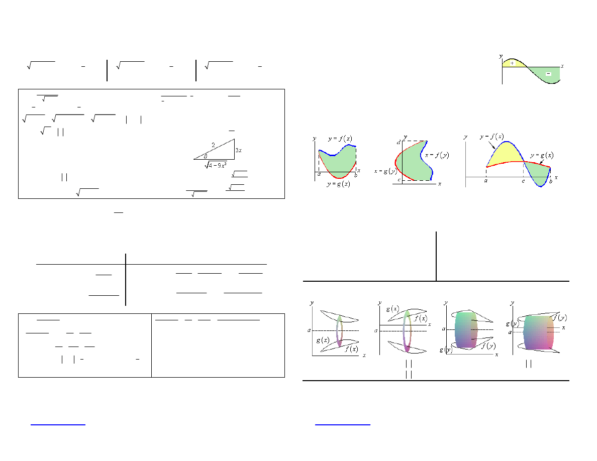
Use Right Triangle Trig to go back to x’s. From
substitution we have
3
2
sin
x
q
=
so,
From this we see that
2
4 9
3
cot
x
x
q
-
=
. So,
2
2
2
16
4 4 9
4 9
x
x
x
x
dx
c
-
-
= -
+
ò
Partial Fractions : If integrating
( )
( )
P x
Q x
dx
ò
where the degree of
( )
P x is smaller than the degree of
( )
Q x . Factor denominator as completely as possible and find the partial fraction decomposition of
the rational expression. Integrate the partial fraction decomposition (P.F.D.). For each factor in the
denominator we get term(s) in the decomposition according to the following table.
Factor in
( )
Q x Term in P.F.D Factor in
( )
Q x
Term in P.F.D
ax b
+
A
ax b
+
(
)
k
ax b
+
(
)
(
)
1
2
2
k
k
A
A
A
ax b
ax b
ax b
+
+ +
+
+
+
L
2
ax
bx c
+
+
2
Ax B
ax
bx c
+
+
+
(
)
2
k
ax
bx c
+
+
(
)
1
1
2
2
k
k
k
A x B
A x B
ax
bx c
ax
bx c
+
+
+ +
+
+
+
+
L
Ex.
2
(
)(
)
2
1
4
7
13
x
x
x
x
dx
-
+
+
ò
(
)
( )
2
2
2
2
(
)(
)
2
1
3
2
2
2
3 16
4
1
1
4
4
3
16
4
1
4
4
7
13
4 ln
1
ln
4
8 tan
x
x
x
x
x
x
x
x
x
x
x
x
dx
dx
dx
x
x
-
+
-
-
+
+
-
+
+
+
=
+
=
+
+
=
- +
+ +
ò
ò
ò
Here is partial fraction form and recombined.
2
2
2
2
4) (
) (
)
(
)(
)
(
)(
)
2
1
1
1
4
4
1
4
(
7
13
Bx C x
x
x
x
x
x
x
A x
Bx C
A
x
x
+ +
+
-
-
-
+
+
-
+
+
+
=
+
=
Set numerators equal and collect like terms.
(
)
(
)
2
2
7
13
4
x
x
A B x
C B x
A C
+
=
+
+
-
+
-
Set coefficients equal to get a system and solve
to get constants.
7
13
4
0
4
3
16
A B
C B
A C
A
B
C
+ =
- =
- =
=
=
=
An alternate method that sometimes works to find constants. Start with setting numerators equal in
previous example :
(
)
(
) (
)
2
2
7
13
4
1
x
x
A x
Bx C
x
+
=
+ +
+
- . Chose nice values of x and plug in.
For example if
1
x
= we get 20 5A
=
which gives
4
A
= . This won’t always work easily.
Calculus Cheat Sheet
Visit
http://tutorial.math.lamar.edu
for a complete set of Calculus notes.
©
2005 Paul Dawkins
Applications of Integrals
Net Area :
( )
b
a
f x dx
ò
represents the net area between
( )
f x and the
x-axis with area above x-axis positive and area below x-axis negative.
Area Between Curves : The general formulas for the two main cases for each are,
( )
upper function
lower function
b
a
y
f x
A
dx
é
ù
é
ù
ë
û
ë
û
=
Þ
=
-
ò
&
( )
right function
left function
d
c
x
f y
A
dy
é
ù
é
ù
ë
û
ë
û
=
Þ
=
-
ò
If the curves intersect then the area of each portion must be found individually. Here are some
sketches of a couple possible situations and formulas for a couple of possible cases.
( ) ( )
b
a
A
f x
g x dx
=
-
ò
( ) ( )
d
c
A
f y
g y dy
=
-
ò
( ) ( )
( )
( )
c
b
a
c
A
f x
g x dx
g x
f x dx
=
-
+
-
ò
ò
Volumes of Revolution : The two main formulas are
( )
V
A x dx
=
ò
and
( )
V
A y dy
=
ò
. Here is
some general information about each method of computing and some examples.
Rings
Cylinders
(
)
(
)
(
)
2
2
outer radius
inner radius
A
p
=
-
(
) (
)
radius width / height
2
A
p
=
Limits: x/y of right/bot ring to x/y of left/top ring
Limits : x/y of inner cyl. to x/y of outer cyl.
Horz. Axis use
( )
f x ,
( )
g x ,
( )
A x and dx.
Vert. Axis use
( )
f y ,
( )
g y ,
( )
A y and dy.
Horz. Axis use
( )
f y ,
( )
g y ,
( )
A y and dy.
Vert. Axis use
( )
f x ,
( )
g x ,
( )
A x and dx.
Ex. Axis :
0
y a
= >
Ex. Axis :
0
y a
= £
Ex. Axis :
0
y a
= >
Ex. Axis :
0
y a
= £
outer radius :
( )
a f x
-
inner radius :
( )
a g x
-
outer radius:
( )
a
g x
+
inner radius:
( )
a
f x
+
radius : a y
-
width :
( ) ( )
f y
g y
-
radius : a
y
+
width :
( ) ( )
f y
g y
-
These are only a few cases for horizontal axis of rotation. If axis of rotation is the x-axis use the
0
y a
= £ case with
0
a
= . For vertical axis of rotation (
0
x a
= > and
0
x a
= £ ) interchange x and
y to get appropriate formulas.
Calculus Cheat Sheet
Visit
http://tutorial.math.lamar.edu
for a complete set of Calculus notes.
©
2005 Paul Dawkins
Work : If a force of
( )
F x moves an object
in a x b
£ £ , the work done is
( )
b
a
W
F x dx
=
ò
Average Function Value : The average value
of
( )
f x on a x b
£ £ is
( )
1
b
avg
a
b a
f
f x dx
-
=
ò
Arc Length Surface Area : Note that this is often a Calc II topic. The three basic formulas are,
b
a
L
ds
=
ò
2
b
a
SA
y ds
p
=
ò
(rotate about x-axis)
2
b
a
SA
x ds
p
=
ò
(rotate about y-axis)
where ds is dependent upon the form of the function being worked with as follows.
( )
( )
2
1
if
,
dy
dx
ds
dx
y
f x
a x b
=
+
=
£ £
( )
( )
2
1
if
,
dx
dy
ds
dy
x
f y
a
y b
=
+
=
£ £
( )
( )
( )
( )
2
2
if
,
,
dy
dx
dt
dt
ds
dt
x
f t y g t
a t b
=
+
=
=
£ £
( )
( )
2
2
if
,
dr
d
ds
r
d
r
f
a
b
q
q
q
q
=
+
=
£ £
With surface area you may have to substitute in for the x or y depending on your choice of ds to
match the differential in the ds. With parametric and polar you will always need to substitute.
Improper Integral
An improper integral is an integral with one or more infinite limits and/or discontinuous integrands.
Integral is called convergent if the limit exists and has a finite value and divergent if the limit
doesn’t exist or has infinite value. This is typically a Calc II topic.
Infinite Limit
1.
( )
( )
lim
t
a
a
t
f x dx
f x dx
®¥
¥
=
ò
ò
2.
( )
( )
lim
b
b
t
t
f x dx
f x dx
-
®-¥
¥
=
ò
ò
3.
( )
( )
( )
c
c
f x dx
f x dx
f x dx
-
-
¥
¥
¥
¥
=
+
ò
ò
ò
provided BOTH integrals are convergent.
Discontinuous Integrand
1. Discont. at a:
( )
( )
lim
b
b
a
t
t a
f x dx
f x dx
+
®
=
ò
ò
2. Discont. at b :
( )
( )
lim
b
t
a
a
t b
f x dx
f x dx
-
®
=
ò
ò
3. Discontinuity at a c b
< < :
( )
( )
( )
b
c
b
a
a
c
f x dx
f x dx
f x dx
=
+
ò
ò
ò
provided both are convergent.
Comparison Test for Improper Integrals : If
( )
( )
0
f x
g x
³
³ on
[
)
,
a
¥ then,
1. If
( )
a
f x dx
¥
ò
conv. then
( )
a
g x dx
¥
ò
conv.
2. If
( )
a
g x dx
¥
ò
divg. then
( )
a
f x dx
¥
ò
divg.
Useful fact : If
0
a
> then
1
a
p
x
dx
¥
ò
converges if
1
p
> and diverges for
1
p
£ .
Approximating Definite Integrals
For given integral
( )
b
a
f x dx
ò
and a n (must be even for Simpson’s Rule) define
b a
n
x
-
D =
and
divide
[ ]
,
a b into n subintervals
[
]
0
1
,
x x ,
[
]
1
2
,
x x , … ,
[
]
1
,
n
n
x
x
-
with
0
x
a
= and
n
x
b
= then,
Midpoint Rule :
( )
( ) ( )
( )
*
*
*
1
2
b
n
a
f x dx
x f x
f x
f x
é
ù
» D
+
+ +
ë
û
ò
L
,
*
i
x is midpoint
[
]
1
,
i
i
x
x
-
Trapezoid Rule :
( )
( )
( )
( )
( )
( )
0
1
2
1
2
2
2
2
b
n
n
a
x
f x dx
f x
f x
f x
f x
f x
-
D
»
+
+ +
+ +
+
é
ù
ë
û
ò
L
Simpson’s Rule :
( )
( )
( )
( )
(
)
( )
( )
0
1
2
2
1
4
2
2
4
3
b
n
n
n
a
x
f x dx
f x
f x
f x
f x
f x
f x
-
-
D
»
+
+
+ +
+
+
é
ù
ë
û
ò
L
Wyszukiwarka
Podobne podstrony:
Calculus Cheat Sheet Limits Reduced
Calculus Cheat Sheet Derivatives Reduced
Calculus Cheat Sheet All Reduced
Trig Cheat Sheet Reduced
Algebra Cheat Sheet Reduced
KidWorld GM Cheat Sheet
FFRE Probability Cheat Sheet
php cheat sheet v2
Korean for Dummies Cheat Sheet
impulse studios jquery cheat sheet 1 0
css cheat sheet v2
jQuery 1 3 Visual Cheat Sheet by WOORK
KidWorld GM Cheat Sheet
css cheat sheet
GPG Cheat Sheet
READ ME Morrowind Master Cheat Sheet v3 0
Ben Settle Copywriters Cheat Sheet Sequel
GURPS (4th ed ) Martial Arts Techniques Cheat Sheet
więcej podobnych podstron