
Electronic copy available at: http://ssrn.com/abstract=1804959
1
UNDERSTANDING THE EFECTS OF
VIOLENT VIDEO GAMES ON VIOLENT CRIME
A. Scott Cunningham, Baylor University
Benjamin Engelstätter, Zentrum für Europäische Wirtschaftsforschung
Michael R. Ward, University of Texas at Arlington
Corresponding Author:
Michael R. Ward
Associate Professor
Department of Economics
University of Texas at Arlington
Arlington, TX 76019
(tel) 817-272-3090
(fax) 817-272-3145
ABSTRACT: Video games are an increasingly popular leisure activity. As many of best-selling
games contain hyper-realistic violence, many researchers and policymakers have concluded that
violent games cause violent behaviors. Evidence on a causal effect of violent games on violence
is usually based on laboratory experiments finding violent games increase aggression. Before
drawing policy conclusions about the effect of violent games on actual behavior, these
experimental studies should be subjected to tests of external validity. Our study uses a quasi-
experimental methodology to identify the short and medium run effects of violent game sales on
violent crime using time variation in retail unit sales data of the top 50 selling video games and
violent criminal offenses from the National Incident Based Reporting System (NIBRS) for each
week of 2005 to 2008. We instrument for game sales with game characteristics, game quality and
time on the market, and estimate that, while a one percent increase in violent games is associated
with up to a 0.03% decrease in violent crime, non-violent games appear to have no effect on
crime rates.
JEL Codes: D08, K14, L86
*
Keywords: Video Games, Violence, Crime

Electronic copy available at: http://ssrn.com/abstract=1804959
2
I.
Introduction
Violence in video games is a growing policy concern. The issue has generated six reports
to the US Congress by the Federal Trade Commission (FTC, 2009) and was the subject of a 2011
US Supreme Court decision.
2
Policymaker concern has been motivated by the connection
between violent video game imagery and psychological aggression in video game players,
particularly adolescents. While researchers have documented an effect on aggression in the
laboratory, some have suggested that violent video games are responsible for violent crime such
as school shootings (Anderson 2004).
3
The shortrun effect of violent games on aggression has been extensively documented in
laboratory experiments (Anderson, Gentile and Buckley, 2007). These experiments generally
conclude that media violence is self-reinforcing rather than cathartic. This link has not been
found with crime data however. A recent study by Ward (2011) found a negative association
between county-level video game store growth and the growth in crime rates. Dahl and
DellaVigna (2009) find that popular violent movies caused crime to decrease in the evening and
weekend hours of a movie’s release lasting into the following week, with evidence that violent
movies were drawing men into theaters and away from alcohol consumption. These two studies
suggest the real world relationship between violent media and crime may be more complex than
the results from laboratory studies suggest.
We estimate the reduced form effect of violent video games on violent crime using a
strategy similar to Dahl and DellaVigna (2009). We proxy for video game play using video game
sales information harvested from VGChartz, an industry source tracking the weekly top 50 best-
selling video game titles from 2005 to 2008.
4
The violent content for each video game was
matched using information provided by the Entertainment Software Rating Board (ESRB).
5
Our

3
measure of crime is from the National Incident Based Reporting System (NIBRS) which we use
to create a time series of violent and non-violent crime levels for the periods in question. To
address possible endogeneity of game releases with unobserved determinants of crime, such as
the coincident release of non-gaming violent media, we instrument for weekly game sales with
game characteristics, such as time a game has been on the market and experts’ reviews of each
game in our sample using Gamespot, a video game review aggregation website.
6
Our
identification strategy requires game quality to be uncorrelated with the unobservable
determinants of crime.
Our main finding is that we do not find evidence for a positive effect on crime. Our most
robust evidence supports the opposite conclusion for a negative effect of violent games on crime.
Our basic 2SLS results indicate that violent crimes fall with violent video game popularity but are
virtually unaffected by changes in weekly non-violent video game sales. These results are not
consistent with games causing aggression but are consistent with either violent games having a
cathartic or an incapacitation effect. We estimate the elasticity of violent crime with respect to
violent game sales to be small, on an order of –0.01 to –0.03.
The rest of our paper is organized as follows: Section II provides background; Section III
describes our data and empirical strategy; Section IV describes our empirical findings; and
Section V concludes.
II.
Background
From the sensational crime stories of the 19
th
century (Comstock and Buckley 1883), to
the garish comic books of the early 20
th
century (Hadju 2009), to the contemporary debate over

4
violent games, Americans have always been concerned about the harmful effects of violent media
on children. Unlike comic books and pulp “true crime” stories, violence in media, including
video games, have received substantial attention by psychologists and media specialists.
Anderson and Bushman (2001) and Anderson et al. (2007) discuss hundreds of controlled studies
on the effects of violence in media, whereas the number of studies on violence in print media is
particularly smaller in comparison.
The impact of violent media on crime has three possible theoretical mechanisms, which
we label “aggression,” “incapacitation,” and “catharsis.” The aggression mechanism is based on a
psychological theory called the “general aggression model,” or GAM. GAM posits that violent
video games increase aggressive tendencies. This model generalizes from social learning theory
(Bandura, 1973), script theory (Huesmann, 1998), and semantic priming (Anderson et al., 1998;
Berkowitz & LePage, 1967) through a process of social learning whereby the gamer develops
mental scripts to interpret social situations both before they occur as well as afterwards. This
effect creates reasoning biases, a tendency to jump to conclusions and may even cause
personality disorders (Bushman and Anderson 2002).
7
While GAM suggests that aggression
increases with repeated exposure to violent content, most of the evidence for it comes from short-
run laboratory experiments.
The incapacitation explanation is based on the economic theory of time use (Becker
1965). Many modern video games are time-intensive forms of entertainment involving intense
narratives with complex plots and characterization taking dozens, and sometimes several
hundreds, of hours to complete.
8
Insofar as video game play draws adolescents from other
activities, the time use explanation implies a short-run decrease in violence as individuals
substitute away from outdoor leisure to indoor leisure, but allow for a possible long-run increase

5
in violence as predicted by GAM. The American Time Use Survey (ATUS) indicates that
individuals aged 15-19 spent an average 0.85 hours per weekday playing games and using
computers, but only 0.12 hours reading, 0.11 thinking, and 0.67 in outdoor recreation, such as
sports or exercising. Ward (2012) uses ATUS data to show that, when the currently available
video games’ sales are higher, individuals’ time spent gaming increases significantly while time
spent in class or doing homework falls. Stinebrickner and Stinebrickner (2008) found that
students randomly assigned a roommate in college with a video game console caused them to
study less often, and in turn, perform worse in school.
The catharsis explanation is that video games act as a release for aggression and
frustration so that actual expressions of aggression are reduced. While gamers believe this to be
true (Ferguson et al., 2010; Olson et al., 2008), it is not without controversy. Most cross-sectional
studies fail to find cathartic effects, but none control for selection on unobservables. Denzler et
al. (2008) state rather unequivocally that “social psychological literature lends no support for the
catharsis hypothesis.” They then find that aggression can reduce further aggression when it serves
to fulfill a goal but caution that these results “do not justify violent media.” A possible
physiological mechanism for catharsis comes from evidence that Internet video game playing is
associated with dopamine release that might act to sate the gamer (Han et al., 2007; Koepp et al.
1998). Han et al. (2009) study the similarity of the effects of video game playing and
methylphenidate (i.e., Ritalin) in children with ADHD and suggest that Internet video game
playing might be a means of self-medication.

6
III.
Data and Methodology
The three explanations have different implications for the effects of violent video games
on violent crime. GAM predicts that crime would increase with greater exposure to violent video
games, especially continuous exposure over long time periods, but not with non-violent games.
While GAM should have long-run effects, to date, most evidence comes from short-term
experiments. Incapacitation predicts that crime would decrease in the shortrun with both violent
and non-violent games, perhaps more so for non-violent games not subject to GAM. Catharsis
predicts that crime, especially violent crime, would decrease with violent games, but not with
non-violent games. In this section, we explain how we specify tests for these predictions and the
data sources we employ.
A. Estimation Strategy
We begin by estimating a standard multivariate regression model of the incidence of
various crimes as functions of, among other controls, the prevalence of non-violent and violent
video games. Our outcome variables of interest, C
t
, are the total number of reported criminal
incidents in week t that are classified as violent or non-violent. Any criminal incident may reflect
some level of aggression, but we interpret violent crimes as reflecting more aggression than non-
violent crimes. While the dataset we use documents criminal offenses on a daily basis, since the
video game sales data are available only on a weekly basis, we aggregate crimes into weekly
measures to avoid double counting of responses to stimuli. Accordingly, we employ a simple
least squares estimator so as to more easily instrument for video game exposure.
9
A game purchased by a gamer in one week is often played in subsequent weeks until the
gamer loses interest and moves on to another game. To address this possibility, we experimented

7
with the effect of game sales on crime for up to a lag of six-weeks. Our main explanatory
variables are aggregated current and lagged values of weekly sales volumes for both non-violent
and violent video games. Video games appear to depreciate quickly with use. This may be
because new games are played intensively for a few weeks after purchase and are not replaced
with a new game until after some diminishing returns have been reached, or it may suggest that
firms typically stagger the release dates of games. Given that we do not know the relative
intensity of game play after game purchase, we do not have strong priors on the pattern of
coefficients on these lags. We focus on the cumulative effect of games measured with the volume
of the current week’s sales, along with the various lags of previous weeks’ sales, so as to capture
the effect of higher volume of game play with varying time lag to trigger crime.
Our model of criminal offenses, C
t
, is:
∑
∑
∑
The number of crime incidents depends on the exposure to violent video game sales
and non-
violent games
. The sum over
of
can be interpreted as the cumulative increase in
criminal incidents over the
weeks for an increase in violent video games sold in week t while
the similar sum for
can be similarly interpreted for non-violent video games. We include an
annual trend and weekly seasonal fixed effects to account for secular increases and seasonality in
both video game purchases and crime. Thus, identification of the parameters of interest comes
from within week-of-year variation around the linear trend. Because many video games are
purchased as Christmas gifts, as a check we also analyze the data omitting this season.
Correlations between video game play and crime may or may not reflect a causal
relationship if the unobserved determinants of crime are correlated with the determinants of video
game play. For instance, bad weather such as rain or heavy snow which causes individuals to

8
remain at home would both increase the likelihood of playing video games and decrease the
returns to crime through higher chances of finding a resident at home. Hence, negative
correlations between crime and violent video game play could purely be a consequence of
omitted variable bias. A low opportunity cost of time would affect both video game sales and the
relative return to criminal activity (Jacob & Lefgren, 2003). For example, both video game sales
and the crime rate increase during the summer when most teenagers are out of school.
Additionally, producers of multiple media sources - movies, television, music and video games –
may be simultaneously targeting time periods in which consumers have low opportunity costs of
time that is unobservable to the researcher. If so, we could be attributing to a causal video game
effect what is actually a more general media effect. We address this potential endogeneity of
video games using characteristics of video games, time on the market and expert reviews of each
title, as an instrument for purchases.
Zhu and Zhang (2010) show that consumer reviews of video games are positively related
to game sales. Ratings are valuable pieces of information for video games because games are
complex experience goods for which gamers cannot know their preferences without playing. Our
data on professional ratings contain rich information that communicates the kinds of information
that gamers value in forecasting their beliefs about the game, and as beliefs and anticipation are
drivers of the game sales, we would expect these rating institutions to play important roles in
forming consumer prior beliefs about the game and therefore their purchases. But we also have
some evidence from other industries that would suggest scores would independently cause
purchases to rise, independent of the unobserved factors that cause expert opinion and purchases
to be highly correlated. Reinstein and Snyder (2005) used exogenous variation in Siskel and
Ebert movie ratings due to disruptions in their pair’s reviewing to determine a causal effect on
movie demand. More recently, Hilger et al. (2010) found that randomly assigned expert scores on

9
bottles of wine in a retail grocery store caused an increase in sales for the higher rated, but less
expensive, wines. While these studies do not confirm that there are exogenous forces in video
game ratings that drive consumer purchases, they are suggestive.
Besides the benchmark specification we employ two additional specifications as
robustness checks. These specifications identify specific segments of the population and locations
where we expect a differential gaming-to-violence link, e.g. counties with a high youth
population and crimes committed in proximity of students. We measure criminal incidents using
the National Incident Based Reporting System (NIBRS) as it provides detailed information on the
criminal offense, including the exact date of the incident, some offender characteristics and the
location of the incident. In the first robustness check, we examine how the effect varies by the
fraction of the county population that is 15-24 years old. In our second check, we extend our
estimation procedure to compare the effects on the number of incidents reported on high school
and college campuses to the number committed at other locations.
B. Video Game Data
VGChartz reports US retail video and computer game unit sales for each week’s top 50
selling video console based games each week consistently beginning in 2005.
10
We harvested
these data using a web-scraping program to create a panel of weekly sales by title for the period
from January, 2005 to December, 2008. We matched each game title with information about the
game’s violent content provided by ESRB’s online database. Finally, we matched each game title
with information about game quality from a game review website, Gamspot.com.
Our video game sales dataset consists of 1,117 separate titles over 208 weeks with some
of these titles being the same game for different gaming consoles. In sum, the games are provided
from 47 different publishers and designed for 9 different gaming consoles. While VGChartz

10
includes the top 50 selling console-based games each week, it only covers a portion of all sales in
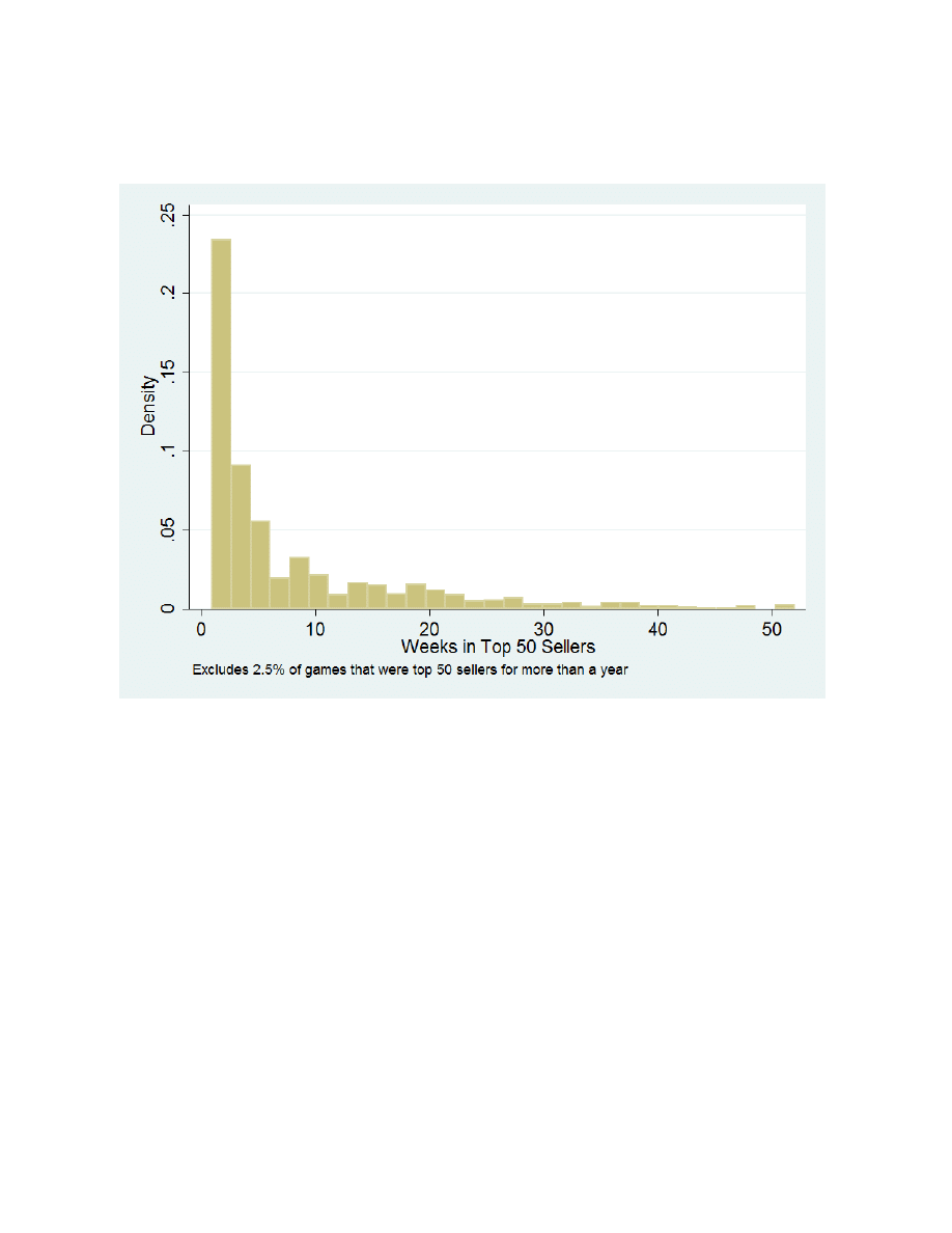
the US video game market. A game’s week of release is almost always its top selling week.
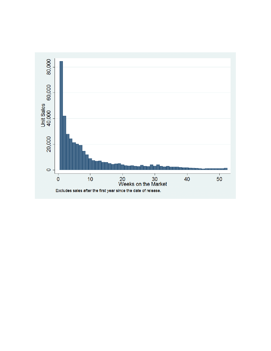
Figure 1 indicates that most games stay in the top 50 for only a few weeks. Moreover, as Figure 2
indicates, games sales by title fall quickly with game age. These features suggest that there is
considerable week-to-week variation in the composition of video games being played. Table 1
compares VGChartz data to the Entertainment Software Association (ESA) and indicates that
VGChartz account for about one-quarter of all units in 2005 (ESA Annual Report, 2010).
11
. The
ESA also includes sales of non-console based games such as computer and smartphone games.
Still, this fraction rises to almost one-half in 2008. While this raises some concerns about
comparability over time, we expect some of this effect to be subsumed into the annual trend.
Insert Table 1 about here
Insert Figure 1 and 2 about here
We record the violence content of each game using the ESRB’s rating and descriptions of
the game’s content. This non-profit body independently assigns a technical rating (E, E10, T, M,
and A) which defines the audience the game is appropriate for where E classifies games for
everybody, E10 for everyone aged 10 and up, T for teens, M games for a mature audience, and A
for adult content. In addition, ESRB provides detailed description of the content in each game on
which the rating was made, including the style of violence, e. g. language, violence, or adult
themes. For all of the 1,117 titles in our sample we collected the appropriate ESRB-rating and all
content descriptors. Based on this content information, we identify 672 non-violent and 445
violent games, of which 113 titles are described as intensely violent. Almost all violent games are
rated T or M. All intensely violent games are rated M. Since most of the policy concern stems

11
from these mature games, we concentrate on the intensely violent games. Merging both data
sources together we can construct measures of the aggregate unit sales of non-violent and
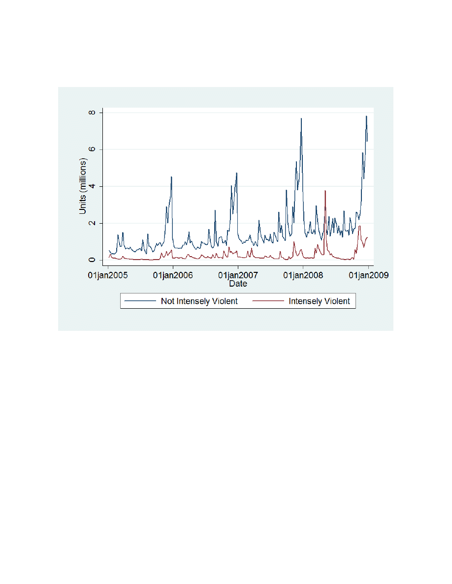
intensely violent video games for each week. The weekly sales are depicted in Figure 3 for all
games and for intensely violent games. Overall, the two graphs follow a similar pattern with a
large peak around the Christmas gift-purchasing period. In the middle of 2008, however, the
intensely violent game sales spiked to account for almost all sales of the violent games.
Insert Figure 3 about here
Our expert review data comes from the GameSpot website. GameSpot provides news,
reviews, previews, downloads and other information for video games. Launched in May 1996
GameSpot’s main page has links to the latest news, reviews, previews and portals for all current
platforms. It also includes a list of the most popular games on the site and a search engine for
users to track down games of interest. The GameSpot staff reviewed all but a handful of the
games in our sample and rated the quality of the titles on a scale from 1 to 10 with 10 being the
best possible rank. These so-called GameSpot-scores assigned to each game are intended to
provide an at-a-glance sense of the overall quality of the game. The overall rating is based on
evaluations of graphics, sound, gameplay, replay value and reviewer’s tilt. GameSpot changed
the rating system in the middle of 2007 and, as a consequence, a game will not get an aspect-
specific rating score anymore. Our examination of overall GameSpot-scores indicates that they
were unaffected by this change in the GameSpot focus. Weekly sales of individual games are
highly sensitive to both game quality and time on the market (Nair, 2007). Accordingly, we
separately aggregate the violent and non-violent games among top 50 games on the market in a

12
week into average GameSpot-scores and average ages, measured in weeks from release, to be
used as instrumental variables.
C. Crime Data
For our measure of weekly crime, we used the NIBRS. NIBRS is a federal data collection
program begun by the Bureau of Justice Statistics in 1991 for gathering and distributing detailed
information on criminal incidents for participating jurisdictions and agencies. Participating
agencies and states submit detailed information about criminal incidents not contained in other
data sets, such as the Uniform Crime Reports. For instance, whereas the Uniform Crime Reports
contain information on all arrests and cleared offenses for the eight Index crimes, NIBRS consists
of individual incident records for all eight index crimes and the 38 other offenses (Part II
offenses) at the calendar date and hourly level (Rantala and Edwards 2000).
Because of the detailed information about the incident, including the precise time and date
of the incident, economists such as Dahl and DellaVigna (2009), Card and Dahl (2009), Jacob
and Lefgren (2003) and Jacob, Lefgren, and Moretti (2007) have used it for event studies. In our
case, we exploit detailed information about the crime’s location for our robustness checks.
One potential drawback of NIBRS is its limited coverage. Unlike the FBI’s Uniform
Crime Reports, only a subset of localities participate. Overall, 32 states currently participate, and
many states with large markets – California, New York, DC – do not participate at all. Moreover,
not all jurisdictions participate within states over time. To address possible selection problems,
we limit our sample to a balanced panel of agencies that participated with NIBRS at the start of
our sample and continued each year.

13
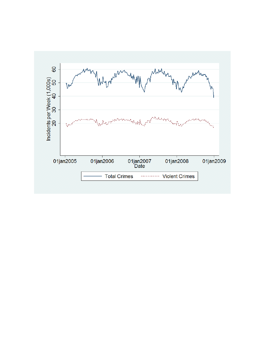
Crimes follow a seasonal pattern. Figure 4 indicates a consistent pattern of gradual
increases in both total and violent crimes from winter to summer. Our method was developed to
account for seasonality in both of our main variables of interest crime and games. Much of the
seasonality in crimes is believed to be due to weather while seasonality in games is likely due to
holiday gift giving (Lefgren, Jacobs and Moretti, 2007). Failure to address these may create
spurious correlations between crime and video game sales. As indicated above, we accommodate
this in two ways. First, weekly dummy variables should capture much of the seasonality. Second,
we use IVs constructed from information on games’ Game Spot Scores as well as how long
games have been on the market to isolate the variation in game sales solely due to the
characteristics of the currently available video games.
Insert Figure 4 about here
D. Final Sample
Our final sample includes 208 weekly observations on video games sales and crimes from
early 2005 through 2008. However, four observations are excluded from final regressions
because of the use of lagged video game sales. Table 2 reports basic descriptive statistics for our
sample.
Insert Table 2 about here
Our method is most like Dahl and DellaVigna (2009), and therefore we contrast our study
to illustrate its strengths and weaknesses. Like Dahl and DellaVigna (2009), we do not have
geographic variation in sales data. Whereas first run movies can be described as non-durables

14
lasting two hours on average, video games are more complex. Unlike feature films, they are
durable goods, being played repeatedly after purchase with actual time use being highly variable
both by title and individual player. Some families budget time allowances for video game play,
while others allow unlimited play time. The time use decision to do so is likely related to the
family characteristics that are correlated with the determinants of crime, such as family structure
and income. Furthermore, box office movie sales are available by day whereas video game data
are only available at the weekly level. Hence one of the reasons we favor our instrumental
variables strategy is that it provides greater confidence in the results by exploiting the variation in
game characteristics to identify exogenous variation in weekly game sales.
IV.
Results
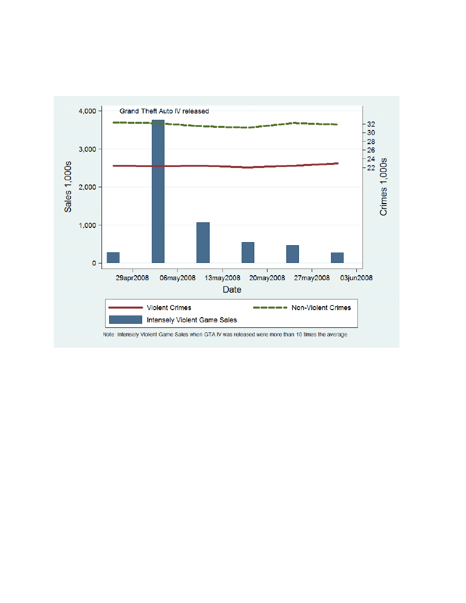
Figure 5 demonstrates the challenges faced by our methodology. When “Grand Theft
Auto IV” was released in on April, 29, 2008 it sold over two million units in its first week. This
was double the weekly sales of any other intensely violent video game in our sample and raised
sales of intensely violent games that week to ten times the sample average (see figure 3 also).
Yet, even with this massive “stimulus,” it is not clear that there was a subsequent “response” in
the number of crimes. Any actual effects are likely to be so small that they are not revealed by
individual events, even large ones.
Insert figure 5 about here
Before proceeding to estimation results, we first conduct tests confirming the stationarity
of the relevant data series after detrending and deseasonalizing each series. We conduct

15
Augmented Dickey-Fuller (ADF) tests for a unit root with four lags. The lag length was chosen
using the Schwarz's Bayesian Information Criterion (SBIC) for various lag lengths. As table 3
reports, we can reject a unit root for the four series representing crimes and video game sales.
Insert table 3 about here
A. Basic Results
Our basic OLS regression results are presented in Tables 4. Table 4 reports estimates of
specifications for four lags of the effect of video games sales, measured in thousands, on violent
crimes and on all crimes. Video games are separated between those that the ESRB rated as
“intensely violent” and those that are not. Recall that the lesser rating of merely “violent” does
not warrant an ESRB rating of “Mature.”
13
Control variables include 52 weekly dummies to
capture seasonality and a year trend to capture a possible spurious correlation due to an upward
trend in games sales and a downward trend in crime. The specification reported here includes
four lags of game sales. Higher order lags failed to achieve significance but specifications with
either more or fewer lags generated similar overall results. While the non-violent video game
sales variables display no obvious pattern, those for violent video games are all negative.
With this this many lags and with lag values possibly being correlated, we do not expect
to be able to distinguish the effect of one week from the next. Instead, we concentrate on the
cumulative effect over all lags. F tests for the cumulative effect over all four lags, reported in the
first two columns of the top panel of table 5, indicate that violent games are associated with
reductions in both the violent and all crime outcome measures. These effects are consistent only

16
with the hypothesized cathartic effect from violent video games. However, the estimated effect is
small, implying an average elasticity of crime with respect to violent games of about -0.01.
Insert Tables 4 and 5 about here.
B. Results without the Christmas season
One concern is that the lag structure from purchase to playing to effects on crime will
differ during the Christmas gift-giving season. Many purchases made weeks before Christmas
will not be played until after Christmas. This is above and beyond the seasonality shift effects we
expect the weekly dummy variables to capture. To address this, we re-estimate the basic model
but omit the last four weeks and first two weeks of the calendar year. Rather than report
coefficients of all lag values, we report the cumulative effects in the bottom panel of table 5.
These results are not very different from those that include the Christmas season.
C. Instrumental Variable Results
As mentioned above, it could be possible that the release of different types of games
coincides with other possible factors affecting crime. For example, demand for various multiple
media may be higher during periods when the target audience has low opportunity cost of time
not accounted for by seasonality. If so, the actual effect on crime may be due to an omitted
variable and not playing video games. To attempt to address this issue, we repeat our analysis
with a 2SLS estimator using average game quality and time on the market as instruments. In this
way the variation in video game sales will be related to these product characteristics and not

17
necessarily to demand side factors. With four lags of two variables, we instrument for eight
endogenous variables. Table 6 reports first stage results for video game sales lagged 1 week. For
both violent and non-violent games, while some other lags may be significant, increases in
contemporaneous average quality and age tend to significantly increase and decrease sales
respectively.
14
Table 7 indicates significant variation in all eight endogenous variables emerging
from the instruments.
Table 8 reports the second stage results to the same specification as the OLS regressions
in table 4. Note that Sargan’s statistic fails to reject the null hypothesis that the instruments are
valid. These results generate a pattern similar to the OLS results of table 4, but generally with
larger, in absolute value, coefficient estimates. The cumulative effects are reported in the right
two columns of table 5, both including and excluding the Christmas season. These indicate that
violent video games are associated with reductions in crimes but non-violent video games have
no effect. The implied elasticity of crime with respect to violent video game sales is now -0.015
to -0.028, a larger reduction in crime from violent video game sales than the OLS estimates
indicate.
Insert Tables 6, 7 and 8 about here.
D. Results by County Youth Population
A potential robustness check is to test for differential effects of video games on criminal
offences by the age profile of an area. While the age profile of video game players is increasing,
video games are still primarily played by children, teens and younger adults and not more mature
adults. If younger people play more video games then areas with higher concentrations of

18
younger people should be more affected by video game playing. We distinguish between areas
with high or low concentrations of potential video game players by calculating the fraction of
each county’s population aged between 15 and 25. We separate the counties with a fraction above
the mean of 14.1% from those with a fraction below the mean. Under the assumption that this age
group plays video games more, our model should find that the measured effects will be larger for
counties with a high youth population.
The results of this robustness check are reported in table 9. This table reports results from
the 2SLS estimator but the OLS results are qualitatively similar. Except for disaggregating the
dependent variables by age profile, the specification is identical to that of table 8. Moreover,
across all columns, the overall results are similar to those from table 8. The key difference is the
magnitude of the implied elasticities of violent video games on crime for the low youth versus
high youth counties. For violent crimes, the reduction in crimes when violent video game demand
is high is about 60% higher in high youth counties. However, for all crimes, the reduction in
crimes when violent video game demand is high is about 40% lower in high youth counties.
Thus, this robustness check yields mixed results.
Insert Table 9 about here
E. On Campus Results
Another potential robustness check is to distinguish between crimes committed at schools
and colleges and those committed elsewhere. Schools and colleges tend to be highly
disproportionately populated with people who are of video game playing age. The NIBRS data
record the location of each incident as a categorical variable where one possible choice out of

19
eleven is “school or college campus.” One advantage of this variable over using the age profile of
the county is that the vast majority of on campus crimes will be committed by the population that
disproportionately plays video games. A disadvantage is that many of the younger video gamers
also commit crimes away from schools.
Table 10 reports the results of this robustness check. This table also reports results from
the 2SLS estimator but the OLS results are qualitatively similar. Again, except for disaggregating
the dependent variables by location of the crime, the specification is identical to that of table 8
and the overall results are similar to those from table 8. The robustness test focuses on magnitude
of the implied elasticities of violent video games across the two groups. For both violent crimes
and all crimes, the reduction in crimes when violent video game demand is about twice as high
on campus than off campus. Thus, this robustness check provides further evidence that our basic
result is not due to spurious correlations.
Insert Table 10 about here
V.
Conclusion
Regulation of the content of video games is usually predicated on the notion that the
industry has large and negative social costs through games’ effect on aggression. Many
researchers have argued that these games may also have caused extreme violence, such as school
shootings, because of the abundance of laboratory evidence linking violent media to measured
psychological aggression. Yet to date, because the field has not moved beyond suggestive
laboratory studies, we argue their external validity to understanding the impact on crime is
limited. With the exception of Ward (2011), social scientists have yet to move beyond the

20
laboratory to understand whether concerns about game violence’s causal effect on crime are
warranted. Similar to Dahl and DellaVigna (2009) our evidence finds robust evidence that
violence in media may even have social benefits by reducing crime. Consistent with these
studies, we find that the short and medium run social costs of violent video games may be
considerably lower, or even non-existent. The measured effect stemming from only violent video
games and not non-violent games is consistent with catharsis and not with incapacitation.
Our results are not completely inconsistent with GAM. Most theories in GAM are related
to long term exposure to violent media. Our tests measure only short-term responses to video
game violence. It is possible that there exists a long-term GAM effect as well as a short-term
cathartic effect. The case for regulatory intervention depends on whether both of these effects
apply. While some early work has been done on the long-term effects of video game play, nearly
all the laboratory evidence that currently exists has only uncovered very short-term effects.
15
Our findings also suggest unique challenges to game regulations. GAM proposes that the
individuals playing violent video games are developing, accidentally, a biased hermeneutic
towards people wherein they believe they are in danger. It is possible that the decrease in violent
outcomes that we observe in our study, possibly due to short-run catharsis, is masking the long-
run harm to society if these violent behaviors are developing within gamers. This suggests that
regulation aimed at reducing violent imagery and content in games could in the long-run reduce
the aggression capital stock among gamers, but potentially also cause crime to increase in the
short-run if the marginal player is currently being drawn out of violent activities. This tradeoff
may not pass a cost-benefit test.
A related policy question centers on whether reducing violent content of video games so
as to diminish GAM related aggression effects also would diminish any time use and cathartic

21
effects. Presumably, publishers include content that is violent because there is a market niche that
demands it. They believe that removing the violence would lower profits because it would reduce
these gamers’ willingness-to-pay. It is not clear how much time use might fall, but lower utility
from such games would reduce game demand and game play time by some amount. The ability to
craft a regulation restricting violent content that does not also lower consumer utility seems
remote.
Using our approach we find a negative inelastic relationship between weekly non-violent
video game sales and weekly crime of no more than –0.03. As our research design exploits
shortrun variation in weekly sales up to a four week lag, caution should be used in applying it
outside our sample frame. For instance, if behavioral effects from popular, higher quality games
diverge from that of popular, lower quality games, then our approach may misstate the average
elasticity of games independent of quality. Furthermore, our elasticity is exclusively based on
shortrun variation in sales, which may be different from effects in the longrun. For instance, the
substitution out of schooling to video gameplay as Stinebrickner and Stinebrickner (2008) and
Ward (2012) show might imply that longrun effects of violent games on crime are positive by
reducing human capital and wages (Grogger 1998). With this caveat, we use this elasticity to
construct a simple counterfactual for US crimes from 2005 to 2008.
To provide context for the magnitude of our estimated effects, we consider a simple back-
of-the-envelope calculation using the numerical growth in video game sales over our sample
period. From Table 1, we calculate that video game unit sales increased by an average of 9.6%
per year. Assuming this applies to both violent and non-violent games, our estimated violent
video game-to-violent crime elasticity of approximately -0.03 would predict almost 0.3% fewer
violent crimes per year due to violent video game sales. Nationwide, this would translate to about

22
10 fewer violent crimes committed per day.
16
By comparison, the estimated incapacitation effect
from Jacob and Lefgren (2003) of 13.3% more property crimes due teacher in-service days,
would translate into about 2,300 property crimes for a hypothetical national in-service day.
17
Since the video game effect occurs year round, this suggests that there are potentially large social
externalities associated with crime that violent games are disrupting in the shortrun.
This approach can help guide investigators to develop more holistic research designs, such
as field experimentation and other quasi-experimental methodologies, to determine the net social
costs of violent games. The main shortcoming of our approach is due to the limitations of our
data on game sales. Unfortunately, the industry does not report cross-sectional variation in game
sales – only the national weekly sales of the top 50 highest grossing games are available. As a
result, our paper follows a methodology similar to Dahl and DellaVigna (2009), who estimated
the impact of violent movies, as proxied by daily ticket sales, on crime using only time series
methods. These analyses are suggestive of the hypothesis that violent media paradoxically may
reduce violence in the short-run while possibly increasing the aggressiveness of individuals in the
long-run.

23
References
Anderson, Craig A. (2004). “An update on the effects of playing violent video games,” Journal of
Adolescence 27, 113–122.
Anderson, C. A., Benjamin Jr., A. J., & Bartholow, B. D. (1998). Does the gun pull the trigger?
Automatic priming effects of weapon pictures and weapon names. Psychological Science,
9, 308–314.
Anderson, Craig A, Douglas A. Gentile, Katherine E. Buckley. (2007) Violent video game effects
on children and adolescents: theory, research and public policy. Oxford University Press,
1st edition.
Anderson, C. A. and B. J. Bushman. 2001. “Human aggression.” Annual Review of Psychology,
53:27–51.
Bandura, A. (1973). Aggression: A social learning analysis. Englewood Cliffs: Prentice Hall.
Becker, Gary S. (1965). “A theory of the allocation of time.” Economic Journal 75 (299), pp.
493-517.
Becker, Gary and Kevin M. Murphy (1988). “A theory of rational addiction.” The Journal of
Political Economy 96: p. 675-700.
Berkowitz, L., & LePage, A. (1967). “Weapons and aggression eliciting stimuli.” Journal of
Personality and Social Psychology, 7, 202–207.
Bushman, B. J. and C. A. Anderson (2002). “Violent video games and hostile expectations: a test
of the general aggression model.” Personality and Social Psychology Bulletin 28 (12):
1679-1686.
Card, David and Gordon B. Dahl (2011). “Family violence and football: the effect of unexpected
emotional cues on violent behaviour.” Quarterly Journal of Economics (forthcoming).
Comstock, Anthony and J. M. Buckley (1883) Traps for the young. Republished in 1967 by
Beknap Press, First Edition.
Dahl, Gordon and Stefano DellaVigna (2009). “Does movie violence increase violent crime?”
Quarterly Journal of Economics, 124(2) 637–675.
Denzler, Markus, Förster, Jens and Liberman, Nira (2008). How goal-fulfillment decreases
aggression. Journal of Experimental Social Psychology 45 (1): 90-100.
Federal Trade Commission. 2009. “Marketing Violent Entertainment to Children: A Sixth
Follow-Up Review of Industry Practices in the Motion Picture, Music Recording &
Electronic Game Industries: A Federal Trade Commission Report to Congress.”
Washington, DC. <
http://www.ftc.gov/os/2009/12/P994511violententertainment.pdf
>.
Ferguson, C. J. and J. Kilburn (2008). “The public health risks of media violence: a meta-analytic
review.” The Journal of Pediatrics 154(4): 759−763.

24
Ferguson, Christopher J., Cheryl K. Olson, Lawrence A. Kutner, and Dorothy E.Warner
(forthcoming) "Violent Video Games, Catharsis Seeking, Bullying, and Delinquency: A
Multivariate Analysis of Effects," Crime & Delinquency.
Grogger, Jeff (1998). “Market wages and youth crime”. Journal of Labor Economics 16(4)
October: 756-791.
Hadju David (2009), The ten-cent plague: the great comic-book scare and how it changed
america. New York: Farrar, Strauss and Giroux.
Han DH, Lee YS, Yang KC, Kim EY, Lyoo IK, Renshaw PF. (2007). “Dopamine genes and
reward dependence in adolescents with excessive internet video game play.” Journal of
Addiction Medicine 1(3), 133-8.
Han, Doug Hyun, Young Sik Lee, Churl Na, Jee Young Ahn, Un Sun Chung, Melissa A. Daniels,
Charlotte A. Haws, Perry F. Renshaw (2009). “The effect of methylphenidate on Internet
video game play in children with attention-deficit/hyperactivity disorder.” Comprehensive
Psychiatry 50, 251–256.
Hilger, James, Greg Rafert and Sofia Villas-Boas (2010). “Expert opinion and the demand for
experience goods: an experimental approach in the retail wine market.” Review of
Economics & Statistics, forthcoming.
Huesmann, L. R. (1998). The role of social information processing and cognitive schema in the
acquisition and maintenance of habitual aggressive behavior. In R. G. Geen & E.
Donnerstein (Eds.), Human aggression: Theories, research and implications for policy
(pp. 73–109). New York: Academic.
Jacob, B. A., and L. Lefgren (2003). “Are idle hands the devil's workshop? incapacitation,
concentration, and juvenile crime.” The American Economic Review 93 (5): 1560-1577.
Jacob, B. A., L. Lefgren and E Moretti (2007). “The dynamics of criminal behavior: evidence
from weather shocks.” Journal of Human Resources 42 (3): 489–527.
Koepp MJ, Gunn RN, Lawrence AD, Cunningham VJ, Dagher A, Jones T, Brooks DJ, Bench CJ
and Grasby PM (1998) “Evidence for striatal dopamine release during a video game.”
Nature 393, 266-8.
Nair, Harikesh (2007). "Intertemporal price discrimination with forward-looking consumers:
Application to the US market for console video-games," Quantitative Marketing and
Economics, 5(3), 239-292.
Olson, Cheryl K., Lawrence A. Kutner, and Dorothy E. Warner (2008). "The Role of Violent
Video Game Content in Adolescent Development Boys’ Perspectives.” Journal of
Adolescent Research 23(1), 55-75.
Rantala, Ramona R and Thomas J. Edwards (2000). “Effects of NIBRS on crime statistics”. NCJ
Publication 178890. US Department of Justice.

25
Reinstein, D. and C. Snyder (2005). “The influence of expert reviews on consumer demand for
experience goods: A case study of movie critics.” Journal of Industrial Economics 53(1):
27–51.
Stinebrickner, Ralph and Todd R. Stinebrickner (2008). “The causal effect of studying on
academic performance.” The B.E. Journal of Economic Analysis & Policy: Frontiers 8(1)
Article 14.
Ward, Michael R. (2011). “Video games and crime.” Contemporary Economic Policy. 29(2) 261-
273.
Ward, Michael R. (2012). “Does time spent playing video games crowd out time spent
studying?,” http://papers.ssrn.com/sol3/papers.cfm?abstract_id=2061726.
Zhu, Feng and Xiaoquan (Michael) Zhang (2010). “Impact of online consumer reviews on sales:
the moderating role of product and consumer characteristics.” Journal of Marketing, Vol.
74 (March 2010), 133–148.
26
Figure 1
Number of Weeks a Game is in the Top 50 Sellers
27
Figure 2
Average US Video Game Unit Sales by Weeks after Release
28
Figure 3
Weekly Sales of Video Games
29
Figure 4
Total and Violent Crimes by Week
30
Figure 5
Intensely Violent Video Game Sales and Crimes Around the Release of Grand Theft Auto IV

31
Table 1
Comparison of Unit Sales of Video Games (millions) from
VGChartz and the Entertainment Software Association (ESA)
Year
VGChartz
Entertainment
Software
Association
Percent
2005
56.7
226.3
25.1%
2006
76.2
240.7
31.7%
2007
107.0
267.8
40.0%
2008
141.3
298.2
47.4%
VGChartz from authors’ calculations and ESA from
http://www.theesa.com/facts/pdfs/VideoGames21stCentury_2010.pdf.

32
Table 2
Summary Statistics
Variable
Mean
Std. Dev.
Intensely Violent Video Game Sales (1,000s)
256
373
Not Intensely Violent Video Game Sales (1,000s)
1,572
1,273
Average Intensely Violent GameSpot Score
8.584
0.658
Average Not Intensely Violent GameSpot Score
7.420
0.662
Average Intensely Violent Weeks on Market
18.6
13.8
Average Not Intensely Violent Weeks on Market
18.0
9.8
Violent Crimes
19,639
1,601
All Crimes
49,491
4,168
Violent Crimes in High Youth Counties
7,377
584
Violent Crimes in Low Youth Counties
12,263
1,050
All Crimes in High Youth Counties
30,586
2,714
All Crimes in Low Youth Counties
18,905
1,500
Violent Crimes on Campuses
871
338
Violent Crimes Not on Campuses
20,524
1,830
All Crimes on Campuses
1,887
630
All Crimes Not on Campuses
51,628
4,667
Descriptive statistics of the 208 observations used in later tables.

33
Table 3
Tests of Time Series Stationarity
Variable
Z value
Violent Crimes
-3.132*
All Crimes
-3.688**
Violent Video Game Sales
-4.430**
Non-Violent Video Game Sales
-3.475+
The null hypothesis is that there is a unit root in de-seasoned
and de-trended time series data. We report the results of
Augmented Dickey-Fuller tests for a unit root with four lags.
Lag length determined by Schwarz's Bayesian information
criterion (SBIC).
+ significant at 10%; * significant at 5%; ** significant at 1%

34
Table 4
Ordinary Least Squares (OLS) Results of Video Game Sales on Crime
Violent
Crimes
All
Crimes
Non-Violent Video Game
Sales Lagged 1 week
-0.011
-0.026
(0.108)
(0.229)
Non-Violent Video Game
Sales Lagged 2 weeks
-0.066
-0.206
(0.109)
(0.231)
Non-Violent Video Game
Sales Lagged 3 weeks
0.100
0.168
(0.109)
(0.232)
Non-Violent Video Game
Sales Lagged 4 weeks
-0.201+
-0.368
(0.109)
(0.231)
Violent Video Game Sales
Lagged 1 week
-0.117
-0.227
(0.189)
(0.401)
Violent Video Game Sales
Lagged 2 weeks
-0.242
-0.595
(0.198)
(0.420)
Violent Video Game Sales
Lagged 3 weeks
-0.290
-0.543
(0.198)
(0.420)
Violent Video Game Sales
Lagged 4 weeks
-0.239
-0.686+
(0.189)
(0.402)
Year
68.793
-500.642**
(84.221)
(179.011)
Week Dummies
Sign.
Sign.
R-squared
0.891
0.928
Sample includes 204 weekly observations. Specification
includes 52 weekly dummy variables. Standard errors are
in parentheses. ** p<0.01, * p<0.05, + p<0.1

35
Table 5
Summary of Main Results
Including Christmas Season
OLS
2SLS
Violent
Crimes
All
Crimes
Violent
Crimes
All
Crimes
Sum Non-Violent Video Games
Coefficients
-0.179
-0.432
-0.129
-0.016
(0.166)
(0.352)
(0.435)
(0.854)
Sum Violent Video Games
Coefficients
-0.888** -2.051** -2.351** -3.864**
(0.255)
(0.542)
(0.513)
(1.009)
Non-Violent Video Game Elasticity
-0.013
-0.013
-0.010
0.000
Violent Video Game Elasticity
-0.011
-0.010
-0.028
-0.019
Excluding Christmas Season
OLS
2SLS
Violent
Crimes
All
Crimes
Violent
Crimes
All
Crimes
Sum Non-Violent Video Games
Coefficients
-0.036
0.303
0.481
0.946
(0.242)
(0.482)
(0.525)
(0.908)
Sum Violent Video Games
Coefficients
-0.741** -1.909** -2.669** -3.645**
(0.262)
(0.532)
(0.639)
(1.106)
Non-Violent Video Game Elasticity
-0.002
0.007
0.027
0.022
Violent Video Game Elasticity
-0.007
-0.008
-0.027
-0.015
Estimates for the sum of coefficients on lagged terms. Standard errors are in
parentheses. ** p<0.01, * p<0.05, + p<0.10. The implied elasticity of crime with
respect to video game sales is calculated at sample means.

36
Table 6
First Stage Regressions of Video Game Sales lagged 1 week
on Average Video Game Characteristics
Non-Violent Games
Violent Games
Coef.
Std. Err.
Coef.
Std. Err.
Violent Average Quality lagged 1 week
212.49*
(98.75)
143.66*
(59.87)
Violent Average Quality lagged 2 weeks
-82.18
(121.28) -111.07
(73.53)
Violent Average Quality lagged 3 weeks
172.99
(120.24)
-23.96
(72.90)
Violent Average Quality lagged 4 weeks
-147.29
(93.48)
-89.33
(56.67)
Non-Violent Average Quality lagged 1 week
327.51**
(99.93)
40.09
(60.58)
Non-Violent Average Quality lagged 2 weeks
-165.86
(121.80)
-40.31
(73.84)
Non-Violent Average Quality lagged 3 weeks
-13.84
(119.69)
-3.54
(72.56)
Non-Violent Average Quality lagged 4 weeks
-44.93
(95.48)
-7.15
(57.89)
Violent Average Age lagged 1 week
0.55
(5.66)
-14.61**
(3.43)
Violent Average Age lagged 2 weeks
1.24
(6.75)
7.67+
(4.09)
Violent Average Age lagged 3 weeks
-12.80+
(6.85)
-1.72
(4.15)
Violent Average Age lagged 4 weeks
5.51
(5.61)
3.80
(3.40)
Non-Violent Average Age lagged 1 week
-30.63**
(9.07)
6.69
(5.50)
Non-Violent Average Age lagged 2 weeks
21.01*
(9.73)
2.45
(5.90)
Non-Violent Average Age lagged 3 weeks
14.16
(10.02)
2.57
(6.07)
Non-Violent Average Age lagged 4 weeks
19.20+
(9.77)
11.32+
(5.92)
Sample includes 204 weekly observations. Specification includes 52 weekly dummy variables
and an annual time trend. Standard errors are in parentheses. ** p<0.01, * p<0.05, + p<0.1

37
Table 7
Summary Results for Under-Identification in First Stage Regressions
Variable
Shea Partial R
2
Partial R
2
F( 16, 135)
Non-Violent Game Sales lagged 1 week
0.321
0.305
3.71**
Non-Violent Game Sales lagged 2 weeks
0.316
0.312
3.82**
Non-Violent Game Sales lagged 3 weeks
0.316
0.305
3.70**
Non-Violent Game Sales lagged 4 weeks
0.259
0.284
3.34**
Violent Game Sales lagged 1 week
0.180
0.274
3.18**
Violent Game Sales lagged 2 weeks
0.210
0.247
2.77**
Violent Game Sales lagged 3 weeks
0.225
0.286
3.38**
Violent Game Sales lagged 4 weeks
0.187
0.224
2.43**
This table summarizes the explanatory power of the instrument set for each of the
instrumented variables. ** p<0.01

38
Table 8
Two Stage Least Squares (2SLS) Results of Video Game Sales on Crime
Violent
Crimes
All
Crimes
Non-Violent Video Game
Sales Lagged 1 week
-0.292
-0.478
(0.209)
(0.410)
Non-Violent Video Game
Sales Lagged 2 weeks
-0.251
-0.570
(0.212)
(0.417)
Non-Violent Video Game
Sales Lagged 3 weeks
0.394+
0.903*
(0.213)
(0.418)
Non-Violent Video Game
Sales Lagged 4 weeks
0.020
0.130
(0.234)
(0.460)
Violent Video Game Sales
Lagged 1 week
0.196
0.494
(0.488)
(0.958)
Violent Video Game Sales
Lagged 2 weeks
-0.291
-0.453
(0.474)
(0.932)
Violent Video Game Sales
Lagged 3 weeks
-0.572
-0.768
(0.457)
(0.899)
Violent Video Game Sales
Lagged 4 weeks
-1.684**
-3.137**
(0.479)
(0.942)
Year
195.233
-492.913
(181.398)
(356.404)
Week Dummies
Sign.
Sign.
Sargon’s statistic: χ
2
(8)
9.661
10.488
[0.29]
[0.232]
R-squared
0.813
0.894
Sample includes 204 weekly observations. Specification
includes 52 weekly dummy variables. Standard errors are
in parentheses. ** p<0.01, * p<0.05, + p<0.1

39
Table 9
Robustness Check of Crimes on Youth Population of County
Violent Crimes
All Crimes
Low Youth
High Youth
Low Youth
High Youth
Non-Violent Video Game Sales
Lagged 1 week
-0.179
-0.119
-0.186
-0.338
(0.123)
(0.087)
(0.169)
(0.251)
Non-Violent Video Game Sales
Lagged 2 weeks
-0.175
-0.098
-0.241
-0.420
(0.125)
(0.088)
(0.171)
(0.256)
Non-Violent Video Game Sales
Lagged 3 weeks
0.220+
0.135
0.356*
0.407
(0.125)
(0.088)
(0.172)
(0.256)
Non-Violent Video Game Sales
Lagged 4 weeks
0.057
-0.062
-0.019
0.074
(0.138)
(0.097)
(0.189)
(0.282)
Violent Video Game Sales
Lagged 1 week
0.192
0.020
0.226
0.300
(0.288)
(0.202)
(0.394)
(0.588)
Violent Video Game Sales
Lagged 2 weeks
-0.051
-0.218
-0.410
0.003
(0.280)
(0.197)
(0.383)
(0.571)
Violent Video Game Sales
Lagged 3 weeks
-0.356
-0.148
-0.275
-0.413
(0.270)
(0.190)
(0.370)
(0.551)
Violent Video Game Sales
Lagged 4 weeks
-0.891**
-0.721**
-1.452**
-1.829**
(0.283)
(0.199)
(0.387)
(0.578)
2SLS Estimator. Specification includes 52 weekly dummy variables and an annual trend.
Standard errors are in parentheses.
Sum Non-Violent Video Games
Coefficients
-0.077
-0.144
-0.090
-0.277
(0.256)
(0.180)
(0.351)
(0.524)
Sum Violent Video Games
Coefficients
-1.105**
-1.067**
-1.911**
-1.938**
(0.303)
(0.213)
(0.415)
(0.619)
Estimates for the sum of coefficients on lagged terms. Standard errors are in parentheses.
Non-Violent Video Game Elasticity
-0.010
-0.031
-0.008
-0.014
Violent Video Game Elasticity
-0.023
-0.037
-0.026
-0.016
Implied elasticity of crime with respect to video game sales. Calculated at sample means.
** p<0.01, * p<0.05, + p<0.1

40
Table 10
Robustness Check of Crimes on Campuses and off Campuses
Violent Crimes
All Crimes
Off Campus
On Campus
Off Campus
On Campus
Non-Violent Video Game Sales
Lagged 1 week
-0.260
-0.032
-0.414
-0.065
(0.193)
(0.025)
(0.382)
(0.047)
Non-Violent Video Game Sales
Lagged 2 weeks
-0.237
-0.014
-0.524
-0.046
(0.196)
(0.026)
(0.388)
(0.048)
Non-Violent Video Game Sales
Lagged 3 weeks
0.342+
0.052*
0.827*
0.076
(0.196)
(0.026)
(0.389)
(0.048)
Non-Violent Video Game Sales
Lagged 4 weeks
0.013
0.007
0.158
-0.029
(0.216)
(0.028)
(0.428)
(0.053)
Violent Video Game Sales
Lagged 1 week
0.172
0.024
0.430
0.064
(0.450)
(0.059)
(0.892)
(0.110)
Violent Video Game Sales
Lagged 2 weeks
-0.272
-0.019
-0.385
-0.069
(0.438)
(0.057)
(0.867)
(0.107)
Violent Video Game Sales
Lagged 3 weeks
-0.525
-0.047
-0.741
-0.028
(0.422)
(0.055)
(0.837)
(0.103)
Violent Video Game Sales
Lagged 4 weeks
-1.559**
-0.125*
-2.890**
-0.248*
(0.442)
(0.058)
(0.877)
(0.108)
2SLS Estimator. Specification includes 52 weekly dummy variables and an annual trend.
Standard errors are in parentheses.
Sum Non-Violent Video Games
Coefficients
-0.142
0.013
0. 048
-0.064
(0.401)
(0.052)
(0.795)
(0.098)
Sum Violent Video Games
Coefficients
-2.184**
-0.167**
-3.584**
-0.280*
(0.474)
(0.062)
(0.939)
(0.116)
Estimates for the sum of coefficients on lagged terms. Standard errors are in parentheses.
Non-Violent Video Game Elasticity
-0.011
0.024
0.001
-0.053
Violent Video Game Elasticity
-0.027
-0.049
-0.018
-0.038
Implied elasticity of crime with respect to video game sales. Calculated at sample means. **
p<0.01, * p<0.05, + p<0.1

41
Endnotes
*
We wish to thank Stephen Frasure for excellent research assistance. We received helpful comments from Irene
Bertschek, Pierre Mohnens, the 9
th
ZEW ICT Conference, Paris ICT Conference 2011, UT Arlington, Munich ICT
Conference 2012, Middlesex University and UNC Charlotte.
2
In 2010, California passed a law making it a punishable offense for a distributor to sell a banned violent video to a
minor. The US Supreme Court struck down this law in June, 2011.
3
There is disagreement within the psychological literature about the interpretation of psychological laboratory
studies of video game violence (Ferguson & Kilburn, 2008).
4
http://www.vgchartz.com
5
http://www.esrb.org
6
http://www.gamespot.com
7
A variant of the Becker and Murphy (1988)’s rational addiction model may approximate GAM. The key insight for
GAM is that consumption of a good in one particular not only affects current utility directly, but through a capital
stock accumulation mechanism, it also affects future utility indirectly.
8
The website, How Long to Beat,
, provides user-submitted statistics on completion
times. The 2011 blockbuster, The Elder Scrolls V: Skyrim, lists completion times between 100 and 330 hours. The
2008 hit, Grand Theft Auto IV, lists 12 to 162 hours, with the lower bound 12 hours recorded for a “speed trial”
effort to complete the game as fast as possible.
9
Our empirical methodology is in large part based on DellaVigna and Dahl’s (2009) study of the effect of movie
violence on crime.
10
VGChartz uses a variety of sources to collect data. These include manufacturer shipments, data from tracking
firms, retailer and end user polls, and “statistical trend fitting.” While VGChartz reports by global region, e.g. US,
Japan, Europe, Middle East, Africa and Asia, disaggregated sales within a region is not available.
11
http://www.theesa.com – The reported numbers from ESA also include games for personal computers which
amount to about 10 percent of the market each year and are intentionally not included in VGChartz.
13
Unreported regressions comparing games that are either “intensely violent” or “violent” versus all other games
generally yield much less precisely estimated parameters.
14
Unreported results for the other lag structures are similar.
15
Anderson (2004) notes the lack of longitudinal studies of effects of violent video games on aggression and calls for
more studies aimed at investigating the long-term effects. The best evidence we have at present from laboratory
studies is primarily short-run, making our study more suitable for comparison.
16
This is based on a total of over 1.2 million violent crimes reported in the FBI’s “Crime in the United States”
http://www.fbi.gov/about-us/cjis/ucr/crime-in-the-u.s/2010/crime-in-the-u.s.-2010/tables/10tbl01.xls.
17
This is based on 6.2 million annual property crimes reported in the FBI’s “Crime in the United States”
http://www.fbi.gov/about-us/cjis/ucr/crime-in-the-u.s/2010/crime-in-the-u.s.-2010/tables/10tbl01.xls.
Wyszukiwarka
Podobne podstrony:
Glińska, Sława i inni The effect of EDTA and EDDS on lead uptake and localization in hydroponically
The Effect of Childhood Sexual Abuse on Psychosexual Functioning During Adullthood
Microwave drying characteristics of potato and the effect of different microwave powers on the dried
The effects of social network structure on enterprise system success
the effect of water deficit stress on the growth yield and composition of essential oils of parsley
The Effect of Back Squat Depth on the EMG Activity of 4 Superficial Hip
76 1075 1088 The Effect of a Nitride Layer on the Texturability of Steels for Plastic Moulds
Curseu, Schruijer The Effects of Framing on Inter group Negotiation
A systematic review and meta analysis of the effect of an ankle foot orthosis on gait biomechanics a
71 1021 1029 Effect of Electron Beam Treatment on the Structure and the Properties of Hard
On the Effectiveness of Applying English Poetry to Extensive Reading Teaching Fanmei Kong
EFFECTS OF CAFFEINE AND AMINOPHYLLINE ON ADULT DEVELOPMENT OF THE CECROPIA
The effect of temperature on the nucleation of corrosion pit
The Effect of DNS Delays on Worm Propagation in an IPv6 Internet
the effect of interorganizational trust on make or cooperate decisions deisentangling opportunism de
Jóźwiak, Małgorzata; Warczakowska, Agnieszka Effect of base–acid properties of the mixtures of wate
Ebsco Cabbil The Effects of Social Context and Expressive Writing on Pain Related Catastrophizing
The effects of Chinese calligraphy handwriting and relaxation training on carcinoma patients
You Feel Sad Emotion Understanding Mediates Effects of Verbal Ability and Mother Child Mutuality on
więcej podobnych podstron