
A Homogeneous Framework
for
Computational Geometry and Mechanics
David Hestenes
Department of Physics and Astronomy
Arizona State University, Tempe, Arizona, USA
Need: Euclidean
http://modelingnts.la.asu.edu
Can access related websites from this one
geometry supplies essential mathematical
underpinnings for physics, engineering and
Computer-Aided Geometric Design.
Question:
GEOMETRIC ALGEBRA Website:
How should we formulate Euclidean Geometry to
facilitate geometric modeling and analysis
optimize computational efficiency?
A fundamental problem in the Design of Mathematics
1
.
.

Standard model for Euclidean 3-space:
E
3
= R
3
=
{x}
= 3d real vector space
Rigid body motions and symmetries described by
Euclidean group E(3)
x
−→ x
0
= R x + a
Invariant:
(x
)
2
= (x
0
0
)
2
Computations: Require coordinates and Matrices
[x
0
] = [R] [x] + [a]
Drawbacks:
Extraneous information
(from arbitrary choice of coordinates)
Redundant matrix elements
(9
vs.
elements for 3 degrees of freedom)
Difficult to interpret
(parameters mixed in matrix elements)
Computationally inefficient
multiplications)
2
y
y
~
(9 9
3
3
Geometric algebra eliminates need for coordinates:
Canonical form for orthogonal transformations:
R x =
R
R R
x
1
parity
=
1
Reflection represented by a vector a
Ax
Ax
Ax
x
=
axa
1
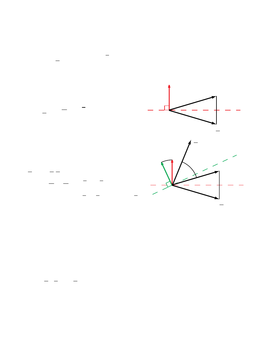
Rotation = double reflection
R x
R x
=
=
BAx
=
b ( axa
1
) b
1
(b a ) x (a
1
b
1
) = R xR
1
Rotation represented by a versor (rotor, spinor, quaternion)
R = ba
Reduces composition of rotations/reflections to
geometric product of versors:
R
2
R
1
= R
3
←
→
R
2
R
1
= R
3
Extensive treatment in (Hestenes 1986)
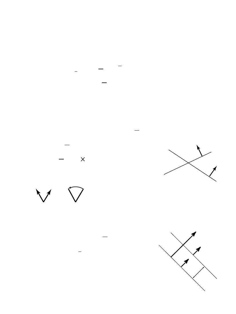
ε
R
ε
+−
a
a
b
x
3
c
π
/3
π
/2
2
2
2
2
b
2
a,
c
a = b = c = 1
4
(
a
b) = 1
b,
a
c
'
b
2
'
3
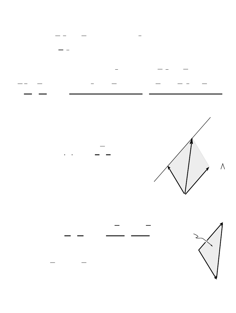
3 Generators:
Symmetries of the Cube
Relations:
(
b
c)
= 1
2
(
c
a)
= 1
a'
π
/4
3
4

Problem:
Vector space model for
E
3
= R
3
=
{x}
singles out one point for special treatment
as the origin x = 0
Drawbacks:
Often need to shift origin to
simplify calculations
avoid dividing by zero
prove results independent of origin
Rigid body displacements combine
rotations multiplicatively and
translations additively,
destroying the simplicity of both
Solution:
Design a homogeneous model for
E
3
that
treats all points equally
treats both rotations and translations multiplicatively
[“homogeneous” in the sense of homogeneous coordinates]
5
~
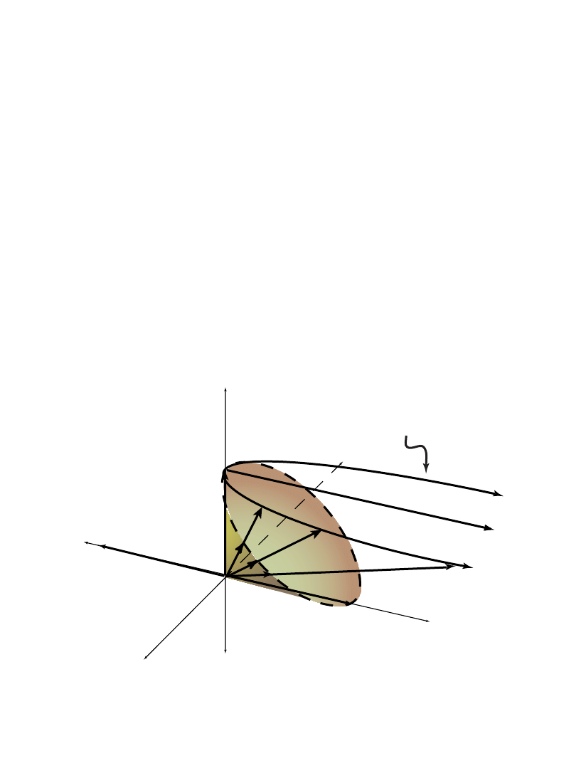
Homogeneous Euclidean Geometry
Arena: Minkowski Algebra
R
n+1,1
=
G(R
n+1,1
)
R
n+1,1
= vector space with signature (n + 1,1)
Null cone:
{x | x
2
= 0
}
Hyperplane:
{x | x e = 1}
Homogeneous model of Euclidean
Geometric algebra essential
space:
E
n
=
{x | x
2
= 0, x e = 1
}
e
2
= 0
x called a point in
E
n
e = point at infinity
Horosphere (F. A. Wachter 1792-1817), (originally with coordinates)
to make the horosphere
coordinate-free
and
computationally efficient
.
e
e
e
0
x
x
e
_
.
.
.
= 1
6
~
Hermann G¨
unther Grassmann (1809-1877)
Laid the foundations for geometric algebra
Set a direction for future development
But he failed to reach his main goal,
ultimately concluding that it was impossible
Grassmann’s Goal:
To formulate
Euclidean geometry as an algebra of geometric objects
(points, lines, planes, circles, etc.)
Interpretation
Computation
The homogeneous model for
E
n
within geometric algebra
reaches Grassmann’s Goal with many surprises!!!
7
integrated
with
married
to
Computational
geometry
Synthetic
geometry
{
}
}
{

Euclidean Geometry is inherent in
algebraic properties of homogeneous points
I. Point-to-point distance from inner products:
(x
y)
2
= x
2
2x y + y
2
=
⇒
=
⇒
Points must be null vectors!
Why Grassmann failed!
Pythagorean theorem, triangular inequality, etc.
II. Lines and Planes from outer products
(another historical curiosity)
III. Geometric relations from algebraic products
e.g.: Point x lies on the line A or plane P if and
and
only if
x
∧ A = 0
A =
A =
x
∧ P = 0
P =
8
a
∧ b ∧ e = line segment or line thru pts a
b
(a
∧ b ∧ e)
2
= (a
b)
2
=
2a b = (length)
2
a
∧ b ∧ c ∧ e = plane segment or plane
(a
∧ b ∧ c ∧ e)
2
=
0
1
1
1
1
0
a b
a c
1
b a
0
b c
1
c a
c b
0
0
0
= 4(area)
2
2
P =
2
Cayley-Menger determinant
Cayley, 1841 (Volumes)
M enger, 1931 (distance geometry)
Dress and Havel, 1993 (relation to GA)
.
.
(x
y)
2
=
2x y
= Euclidean distance
.
.
.
.
.
.
.
The homogeneous model of
is related
to the standard inhomogeneous model by a
Conformal
split:
A 1-to-1 mapping of
E
n
E
n
=
{x}
onto
the pencil of lines
R
n
=
{x}
through a fixed point
e
0
,
defined by
x
−→
x = x
∧ E = x ∧ e
0
∧ e
and the inverse mapping
x
−→
x = xE
1
2
x
2
e + e
0
where
e
0
∧ e = E
=
⇒
E
2
= 1
and
eE = e =
Ee
(absorption)
This implies the isomorphism:
E
n
=
R
n
and determines a split of the whole algebra:
R
n+1,1
=
R
R
n
1,1
where
R
n
=
G(R
n
)
,
and
R
1,1
has the basis:
{1, e, e
0
0
, E = e
∧ e}
9
~
Conformal Splits for Simplexes
Point: a = (a
1
2
a
2
e ) E = E(a
+
1
2
a
2
2
+
e
e
e
)
= aE
1
2
a
2
+ e
e
Product: a b = (aE)(Eb) = (a +
1
2
a
0
0
0
0
0
0
+ e
e
)(b
1
2
b
2
e
e
)
=
1
2
(a
b)
2
+ a
∧ b +
1
2
(a
2
b
b
2
a)e + (b
a)e
1
2
(b
2
a
2
)E
| {z }
|
{z
}
a
a
∧ b
Similar to the mess from the spacetime split in STA
Line (or line segment) thru a, b, e
e
∧
a
∧ b
b
= a
∧ be + (b a)E
|{z}
| {z }
moment
tangent
Pl¨
ucker coordinates
.
a
0
b
a b
Plane (or plane segment)
e
∧
a
∧ b ∧ c
= a
∧ b ∧ ce + (b a) ∧ (c a)E
| {z }
|
{z
}
moment
tangent
a
∧ [(b a) ∧ (c a)] = a ∧ b ∧ c
a
b
c
tangent
.
.
.
1 0
All spheres and hyperspheres
E
n
ar
in
e uniquely
represented b y “positive” vectors in
R
n+1
S
n 1
(
p) = sphere with radius
and center p
represented by vector s with
s
2
(s e)
2
=
2
=
s
s e
1
2
2
e
=
⇒ p
p
2
= 0
Can simplify with constraint s e = 1, so
s
2
=
2
> 0, p = s
1
2
2
e
.
.
x
p
ρ
ρ
ρ
ρ
ρ
ρ
ρ
ρ
ρ
ρ
δ
δ
Eqn. for sphere: x s = 0 ,
x
2
= 0
Conformal split: s = p E +
1
2
(
2
p
2
) e + e
x p =
1
2
2
=
⇒
2
= (x
p)
2
0
H
n 1
(n) = hyperplane rep. by vector n with
n
n e = 0
n
2
= 1
Conformal split: n = n E
=
⇒ n
e
2
= n
2
= 1
Eqn. for hyperplane: x n = 0 , x
2
= 0
or:
x n =
.
(n)
δ
> 0
H
n -1
0
n
.
.
.
.
.
.
.
.
.
.
1 1
,
of
A Surprising algebra
spheres

The homogeneous model of
E
n
maps all spheres and hyperplanes
R
n
into hyperplanes thru the origin in
R
n+1,1
:
{x | x s = 0 , s
2
>
>
0 , s e
0 , x
2
= 0; x, s
∈ R
n+1,1
}
x s = 0
is the eqn for a hyperplane thru the origin
i.e., a (n + 1)-dim subspace of
R
n+1,1
s e = 0
A sphere thru e =
∞ is a hyperplane
Sphere determined by n + 1 points: a
0
, a
1
, a
2
, . . .
. . .
. . .
. . .
. . .
.
.
.
.
.
.
.
.
.
a
n
˜
s
a
0
∧ a
1
∧ a
2
∧
∧ a
n
6= 0
tangent form
tangent form
Radius
I
I
and center p given by duality:
s =
(
(
a
0
∧ a
1
∧ a
2
∧
∧ a
n
)
normal form
normal form
s
s e
2
=
2
,
p =
s
s e
1
2
2
e
Hyperplane = sphere thru
∞, say a
0
= e
˜
n = e
∧ a
1
∧ a
2
∧
∧ a
n
n =
(e
∧ a
1
∧ a
2
∧
∧ a
n
)
)
Eqn for sphere: x
∧ ˜s = 0 ⇐⇒ x s = 0
fl
ρ
ρ
ρ
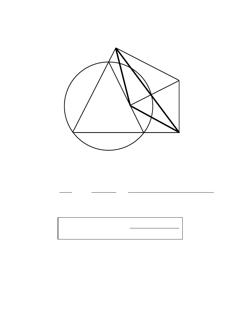
Example: Simson’s construction
.
.
.
.
.
.
.
.
A
A
B
C
C
D
P
1
B
1
1
˜
s
˜
s
= A
∧ B ∧ C = circumcircle of triangle e ∧ A ∧ B ∧ C
ρ
2
=
s
s e
2
=
˜
s
†
˜
s
(
∧ e)
2
=
(
(
C
∧ B ∧ A) (A ∧ B ∧ C)
)
(e
∧ A ∧ B ∧ C)
2
Identity:
(H. Li)
e
∧A
1
∧B
1
∧C
1
=
A
∧ B ∧ C ∧ D
2
ρ
2
A
∧ B ∧ C ∧ D = 0
⇐⇒ e ∧ A
1
∧ B
1
∧ C
1
= 0
D lies on circumcircle
⇐⇒ A
1
, B
1
, C
1
are collinear
.
.
13

Conformal group
on (or )
{
}
E
n
n
Lorentz group
on
{
}
R
n+1,1
n+1,1
=
~
=
~
Versor group
in
{
}
R
R
2
Lorentz Trans. G ( = orthogonal trans.)
G(x) =
Gx G
1
=
σ
σ
σ
parity
=
1
G = versor representation of G
( = spin rep. if
ε
ε
ε
ε
E
= +1)
For homogeneous points
x
0
0
= x
02
= 0,
is a scale factor to enforce
e x
0
x
0
= e x = 1
.
.
.
.
.
.
(not a Lorentz invariant)
Conformal split
G
[x +
1
2
x
2
e + e ]G
1
1
=
[ x
0
+
+
1
2
(x
0
)
2
e + e ]
E
x
0
= g (x) is a conformal trans. on
R
n
Versor rep. reduces composition of conformal transformations
to versor multiplication
g
3
(x) = g
2
[ g
1
(x) ]
⇐⇒
G
3
=
=
G
2
G
1
Versor factors
G = s
k
. . . s
2
s
1
vectors s
2
i
6= 0
Euclidean group E(n) defined by G e G e
14
and
Rigid Displacements
Symmetries
Rotations & translations generated
multiplicatively from reflections
Reflection in the n-(hyper)plane
n
2
= 1
n(x) =
nxn
1
= x
0
σ
= 1
Split form:
= nE
e
δ
n
2
= 1
For plane thru pt c:
n c = 0
=
⇒
δ
= n c
Rotation from planes n and m intersecting at point c:
G = mn = (
E + em c)(nE
en c)
= mn
mn
m
e(m
∧ n) c
= R
e(R
c)
.
.
.
.
.
.
.
.
n
= R
.
n
m
=
R
Spinors as directed arcs
.
c
n
m
T
ranslation
Inversion
from parallel planes m, n
G = mn = (mE
0)(nE + e
δ
)
= 1 +
1
2
ae = T
a
where
a = 2n
δ
generated by sphere vector s
n
δ
n
a
15
SE(3) =
Euclidean group on
E
3
=
{ rigid displacements D} =
2
{spinors D}
D(x) = Dx D
1
D = T R
Translation by c:
T = T
c
= 1 +
1
2
ec
Rotation axis:
n = RnR
†
Chasles’ Theorem: Any rigid displacement can be
expressed as a screw displacement
Proof: Find a point b on the screw axis so that
D = T
c
k
T
c
⊥
R = T
c
k
R
b
= R
b
T
c
k
where
R
b
= R + e b
R ,
c
k
= (c n)
Solution:
b = c
⊥
(1
R
2
)
1
=
1
2
c
⊥
1
R
2
1
h R
2
i
Screw form:
D = e
1
2
S
S = a screw
se(3) = Lie algebra of SE(3) =
{S = in + em}
is a bivector algebra,
closed under
S
1
S
2
=
1
2
(S
1
S
2
S
2
S
1
)
Special
16
.
.
.
˜
Screw theory follows automatically!
Screws:
S
k
=
im
k
+ en
k
Product:
S
1
S
2
= S
1
S
2
+ S
1
S
2
+ S
1
∧ S
2
Transform: S
0
k
= US
k
= U S
k
U
1
= Ad
U
S
k
S
0
1
S
0
2
= U(S
1
S
2
)
Product preserving
.
.
.
.
.
.
.
.
.
.
.
.
.
.
= U (S
1
S
2
+ S
1
S
2
+ S
1
∧ S
2
)U
1
Invariants:
Ue = e ,
Ui = i
=
⇒ U(S
1
∧ S
2
) = S
1
∧ S
2
=
ie(m
1
n
2
+ m
2
n
1
)
S
0
1
S
0
2
= S
1
S
2
=
m
1
m
2
(Killing Form)
Coscrew (Ball’s reciprocal screw)
S
k
=
hSie i
2
0
0
0
0
0
=
1
2
(Sie + ie S) = in
k
+ m
k
e
Invariant: S
1
S
2
= S
2
S
1
=
h (S
1
∧ S
2
) ie
i
= m
1
n
2
+ m
2
n
1
Pitch:
h =
1
2
S
S
S S
= n m
1
*
*
*
*
1 7

Screw Mechanics (of a rigid body)
I Kinematics of body pt.
x = Dx
0
e
0
D
1
D = D(t)
˙
D =
1
2
V D
x
.
= V x
V =
i ω
ω
ω + ev
=
⇒
˙x = ω
ω
ω
x + v
= “instantaneous screw”
v = C M velocity
P = M V = iI ω
ω
ω + mve = i``` + p e
= comomentum
(a coscrew)
II Dynamics
˙
P = W = iΓ + f
= coforce (wrench)
=
⇒
˙
K = V
W = ω
ω
ω Γ + v f = Power
K =
1
2
V
P =
1
2
ω
ω
ω ``` + v p = K.E.
More in NFCM
III Change of Frame
x
−→ x
0
= U x = U x U
1
=
⇒ V
0
= U V
Covariant
˙
U = 0
P = UP
0
Contravariant
P
0
V
0
= P V
Invariant
.
.
.
.
.
.
.
.
.
.
.
.
18
Wyszukiwarka
Podobne podstrony:
Weiss Lie Groups & Quantum Mechanics [sharethefiles com]
Doran & Lasenby PHYSICAL APPLICATIONS OF geometrical algebra [sharethefiles com]
Hestenes Unified Language 4 Maths & Physics (1986) [sharethefiles com]
Dorst & Mann GA a Comp Framework 2 [sharethefiles com]
Dorst & Mann GA a Comp Framework 3 [sharethefiles com]
Dorst & Mann GA a Comp Framework 1 [sharethefiles com]
Doran Geometric Algebra & Computer Vision [sharethefiles com]
Vicci Quaternions and rotations in 3d space Algebra and its Geometric Interpretation (2001) [share
Leon et al Geometric Structures in FT (2002) [sharethefiles com]
Borovik Mirrors And Reflections The Geometry Of Finite Reflection Groups (2000) [sharethefiles com
Rockwood Intro 2 Geometric Algebra (1999) [sharethefiles com]
Buliga Sub Riemannian Geometry & Lie Groups part 1 (2001) [sharethefiles com]
Lasenby GA a Framework 4 Computing Invariants in Computer Vision (1996) [sharethefiles com]
Burstall Isothermic Surfaces Conformal Geometry Clifford Algebras (2000) [sharethefiles com]
Pervin Quaternions in Comp Vision & Robotics (1982) [sharethefiles com]
Lasenby Conformal Geometry & the Universe [sharethefiles com]
Ritter Geometric Quantization (2003) [sharethefiles com]
Doran Grassmann Mechanics Multivector Derivatives & GA (1992) [sharethefiles com]
Apanasov Geometry and topology of complex hyperbolic and CR manifolds (1997) [sharethefiles com]
więcej podobnych podstron