Implementation of a Multi-level Inverter Based on Selective Harmonic

Elimination and Zig-Zag Connected Transformers

Chung-Ming Young, Sheng-Feng Wu, and Yan-Zhong Liu

Department of Electrical Engineering

National Taiwan University of Science and Technology

Taipei, Taiwan, R. O. C 106

Email :

[e-mail]

Abstract—This paper applies the selective harmonic elimination
(SHE) technique to determine the switching angles for a multi-
level inverter that cooperated with specially connected
transformer, zig-zag connection. With the ability to direct
controlling harmonics, SHE technique has the adaptability to
associate with apparatus which are congenitally immune to
specific harmonics, such as the zig-zag connection transformers.
In this paper the two sets of primary windings of the
transformers are supplied by two 6-switch full-bridge inverters
with 30 electrical degrees phase shift. Prohibited by the
transformers, harmonics with orders other than 12n±1 (n is
positive integral) will not appear in the line-to-line voltage of the
secondary side. Then, SHE technique is employed to handle
harmonics with orders equal to 12n±1, and controls the
amplitude of the fundamental. This paper obtains a set of precise
switching angles through off-line calculation and then employs a
digital signal processor to implement on-line calculation of the
switching angles by an approximate method. Some selected
analysis and experimental results are shown in this paper. A
small-size prototype is built to verify the validity of the proposed
system.

Keywords-selective harmonic elilimation (SHE); transformer;

half-wave-symmetry; digital signal processor

I.

I

NTRODUCTION

The technique of selective harmonic elimination (SHE) has

been developed for more than forty years [1],[2]. The primary

advantages of SHE include providing lower switching

frequency, direct controlling harmonic components, and

optimizing particular objects [3]. Thus SHE is a popular

choice among different methods of modulation in many static

power conversion applications [4],[5]. Depending on the

applications, such as the topology of inverters and the number
of phase, there are many perspectives can be used to formulate

the SHE problems [1],[2]. After the problem is formulated, a

set of nonlinear equations, traditionally generated form

Fourier series representation and the optimizing objective

function both based on the specific perspective, has to be

solved before obtaining the desired switching angles. It is well

known that on-line solving these nonlinear equations have

been an obstacle to engineers who are trying to apply SHE

technique in their systems [3],[6]. Moreover, once the number

of variables in the nonlinear equations increases, the burden of

calculating also increases significantly. Thus most SHE

applications use off-line calculation to ease the complication

of the system [5]. To reduce the number of variables, the
output waveforms are always constrained to be symmetric. For

example, by making half-wave-symmetry assumption to SHE

formulations, even harmonics are eliminated automatically.

Furthermore, quarter-wave-symmetry assumption, which

imposes more constraints but requires lesser variables, is more

popular than half-wave-symmetry assumption. With quarter-

wave-symmetry assumption, all harmonics have either 0 or

180 degrees phase shift with respect to the fundamental, while

half-wave-symmetry assumption allows harmonic phasing to

vary [7],[8]. Although the former is convenient for solving the

nonlinear equations, it often results in sub-optimal solutions.

With the ability to direct controlling harmonics in the

output waveform, SHE techniques have the adaptability to

associate with apparatus which are congenitally immune to

specific harmonics, such as the zig-zag connection

transformers. When SHC associates with such electric

apparatus, the strategy of SHE can leave those specific

harmonics uncontrolled or maximize them and focus efforts

on harmonics for which are most concerned. According to this

strategy, either the lowest switching frequency or output

distortion can be achieved.

In some dc/ac applications the output transformers are

deployed to adjust the voltage level between primary and

secondary sides and/or to meet the isolation requirement. For

example, the static inverter (SIV), as shown in Fig. 1, which

provides ac power for air conditioning and lighting on electric

trains in Taiwan, deploys two three-phase transformers with

zig-zag connection in their secondary windings. It can be

shown that ,with this kind of connection, harmonics with
orders other than 12n±1 present in the primary windings will

be trapped in the secondary windings and absent in the line-to-

line voltages of the secondary side.

In this paper, SHE technique with half-wave-symmetry

assumption is investigated to obtain the switching angles for

an inverter system that deploys two zig-zag connection

transformers in output stage. The two sets of primary windings

of the transformers are supplied by two 6-switch full-bridge

inverters with 30 electrical degrees phase shift. As mentioned

above, harmonics with orders other than 12n±1 will not appear

in the line-to-line voltage in the secondary side. Thus, SHE

technique with half-wave symmetry is employed to handle

harmonics with orders equal to 12n±1, and control the

The authors would like to thank the National Science Council for

financial supporting. The work was sponsored by NSC-94-2218-E-011-145

PEDS2009

387

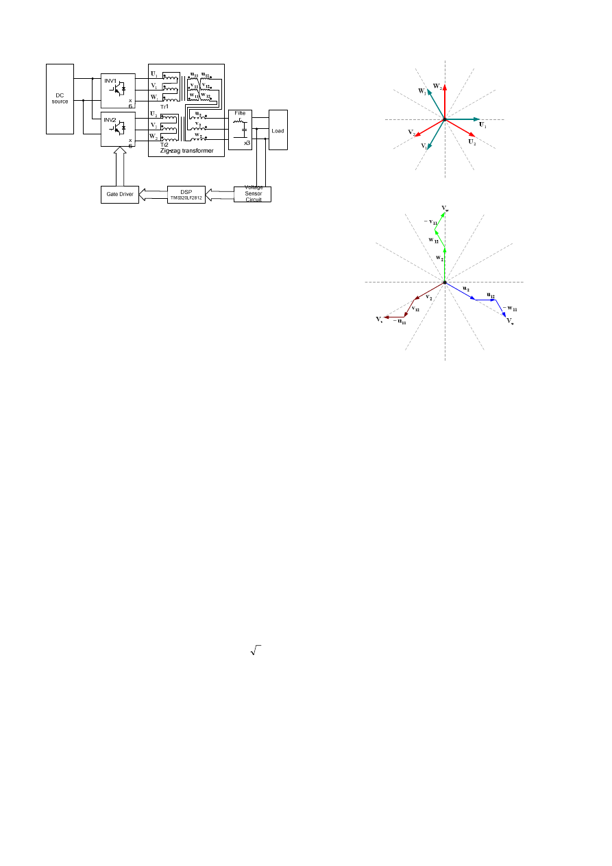
Figure 1. The diagram of the proposed system

(a)

(b)

Figure 2. Fundamental phasor diagrams of zig-zag transformers, (a)

primary,(b) synthesize of secondary

amplitude of the fundamental. The uncontrolled harmonic

profiles of the output waveform obtained under half-wave-

symmetry assumption are different form those with quarter-

wave-symmetry assumption. In other words, it is possible that

the former provides better solutions than the latter in this

application. Based on the strategy that the fundamental is

controllable and 11th and 13th harmonics are eliminated, a set

of full-range (both amplitude and phase of the fundamental)

solutions with three switching angles are obtained. By the

helping of the transformers, we can choose the switching

angles with minimum 23rd and 25th harmonics, which are the

most concerned in this paper. Some selected analysis and

experimental results are shown in this paper. A small-size

prototype is built to verify the practical validity of the

proposed system.

The paper is organized as follows. In section II, the

proposed system and the characteristics of zig-zag transformers

are described. SHE strategy with half-wave-symmetry

assumption is given in section III. The on-line calculation

based on approximate method is presented in Section IV.

Section V shows some experimental results. Conclusions are

summarized in Section VI.

II. S

YSTEM DESCRIPTION AND

C

HARACTERISTICS OF

Z

IG

-

Z

AG

T

RANSFORMERS

Fig. 1 shows the diagram of the proposed system which

includes two inverters, two transformers, and a DSP-based

controller, which executes on-line calculation to obtain the

switching angles and carries out the voltage regulation at the

filtered output. These two transformers, denoted as Tr1 and

Tr2, have delta connections in the primary sides, while the

secondary windings of the Tr1, which has two identical

windings in each phase, employ interconnection and then are

in series with the secondary windings of Tr2. The turn ratio
between secondary windings of Tr1 and Tr2 is

3

:

1

and the

turn ratio between primary and secondary is dependent on

voltage levels of both sides. This special connection of the

secondary windings of the transformers provides immunity

from some harmonics. Before taking this advantage, an

assumption has to make first, that is, these two transformers

have to be supplied by two phase-shifted ac sources with 30

electrical degrees. Under this assumption, Fig. 2 shows the

phasor diagrams of the fundamental voltages of the
transformers.

x

U

,

x

V

and

x

W

, where

1

x

=

and

2

, are denoted

as the primary voltage phasors of Tr1 and Tr2 respectively,
and

11

u

,

11

v

,

11

w

,

12

u

,

12

v

,

12

w

,

2

u

,

2

v

,

2

w

denoted as the

secondary voltage phasors of Tr1 and Tr2 respectively. It can

be seen that the output side (secondary side) is basically in Y-

connection and each phase is composed of three phasors.

Thus, the line-to-line voltages of the secondary side can be

expressed as

2

12

11

11

12

2

uv

v

v

u

w

u

u

V

−

−

+

−

+

=

(1)

2

12

11

11

12

2

vw

w

w

v

u

v

v

V

−

−

+

−

+

=

(2)

2

12

11

11

12

2

wu

u

u

w

v

w

w

V

−

−

+

−

+

=

(3)

where

uv

V

,

vw

V

and

wu

V

are phasors of the line-to-line

voltages of the secondary.

As shown in Fig. 1, the two transformers are individually

supplied by two inverters, denoted as INV1 and INV2, which
receive switching signals from the digital controller. Through
proper time delay, it is easy for the digital controller to
generate switching signals that trig the inverters’ switches and
then provides two balanced three-phase ac sources with 30
degrees phase shift between their fundamentals in spite of the
pulse-width-modulation (PWM) methods. The proposal
switching signals, which are determined by SHE technique,
will be detailed later in this paper.

PEDS2009

388

1

α

2

α

3

α

1

(deg.)

γ

So

lu

tions

(d

eg

.)

i

α

Figure. 3. Solutions

i

α

at a modulation index of 1.0 as

1

γ

varying

from 0

° to 360° with harmonic control of eliminating 11th and 13th

harmonics.

1

φ

2

φ

3

φ

1

(deg.)

γ

Sol

uti

on

s

(de

g.

)

i

φ

Fig. 4. Three corresponding phase-shift angles of each quasi-

square wave at unit modulation index of 1.0 as 1

γ

varying

from 0

° to 360° with harmonic control of eliminating 11th

and 13th harmonics.

T

ABLE

I

C

ALCULATING

uv

V

WITH RESPECT TO DIFFERENT HARMONICS

Order of harmonic

2

u

12

u

11

w

11

u

12

v

2

v

uv

V

1

1.5-j0.866

1

-0.866+j1.5

1

-0.866-j1.5

-1.5-j0.866

6.735

3+12m

-j1.733

1

-1

1

-1

j1.733

0

5+12m

-1.5-j0.866

1

0.5+j0.866

1

0.5-j0.866

-1.5+j0.866

0

7+12m

-1.5+j0.866

1

0.5-j0.866

1

0.5+j0.866

-1.5-j0.866

0

9+12m

j1.733

1

-1

1

-1

-j1.733

0

11+12m

1.5+j0.866

1

-0.5-j0.866

1

-0.5+j0.866

-1.5+j0.866

5.997

13+12m

1.5-j0.866

1

-0.5+j0.866

1

-0.5-j0.866

-1.5-j0.866

5.997

In most case, the output waveforms of the inverters contain

fundamental and several harmonic components as well. As
mentioned above, the phase-shift angle between the
fundamentals of the outputs of INV1 and INV2 is 30 degrees,
that means the fundamental of

1

U

is leading the fundamental

of

2

U

by 30 degrees, while the h-th harmonic of

1

U

is leading

the harmonic of

2

U

by 30

×

h degrees, where h is integer.

Equations (1)-(3) are not only useful to determine the
fundamentals in the line-to-line voltages, but also available to
determine the harmonics, except that different order of
harmonic has different phase angle. By calculating (1)-(3), it
can be proved that harmonics with orders other than 12n

±

1

will not appear in the line-to-line voltage in the secondary side.

Table I shows the calculating results of (1) for harmonics

with and without orders of 12n

±

1. For convenience,

11

u

is

selected as the reference phasor with unit amplitude and zero
phase angle. For harmonics with orders 3+12m,
where

"

2,

,

1

,

0

=

m

, the individual phasor of the six terms in

the left side of (1) have the identical phasor representations and
the results of

uv

V

are all zeros. Moreover, the harmonics with

orders k+12m, where

9

and

7

5,

,

3

=

k

, have similar

formalizations. Nevertheless, the harmonics with orders
11+12m and 13+12m, i.e. 12n

±

1, have non-zero

uv

V

. As all

odd-order harmonics are considered in Table I, it can conclude
form above that harmonics with orders other than 12n

±

1

present in the primary windings will be trapped in the
secondary windings and absent in the line-to-line voltages of

the secondary side. Identical results of calculating

vw

V

and

wu

V

can be obtained from (2) and (3) respectively.

III. SHE

STRATEGY WITH HALF

-

WAVE

-

SYMMETRY

ASSUMPTION

The Fourier series representations of a two-level k-notch

half-wave-symmetric waveform are given by (4) and (5)

4

(2

( 1) cos

sin

)

p

p

k

real

i

h

h

p i

p i

p

i

a

h

h

h

α

φ

π

=

=

−

×

∑

F

∀

h N

∈

(4)

4

(1 2

( 1) cos

cos

)

p

p

k

imag

i

h

h

p i

p i

p

i

b

h

h

h

α

φ

π

= −

= −

+

−

×

∑

F

∀ h N

∈

(5)

where

p

h

is the

p

-th element in a set of controlled

harmonics

N

having

k

elements,

α

is a vector of length

k

with each element

i

α

representing the

i

-th notching,

φ

is a

vector of length

k

with each element

i

φ

representing the

phase-shift angle corresponding to the

i

-th quasi-square wave.

The harmonic content can also be described in polar

coordinates such that

( )

cos

real

h

p

p

F

m

γ

=

(6)

( )

sin

imag

h

p

p

F

m

γ

=

(7)

PEDS2009

389

1

(deg.)

γ

1

m

1

(d

eg

.)

α

1

(deg.)

γ

1

m

1

(d

eg

.)

φ

(a) (b)

1

(deg.)

γ

Modulation index

1

m

2

(d

eg

.)

α

Selected solution trajectory

1

(deg.)

γ

1

m

2

(d

eg

.)

φ

(c) (d)

1

(deg.)

γ

1

m

3

(d

eg

.)

α

1

(deg.)

γ

1

m

3

(d

eg

.)

φ

(e) (f)

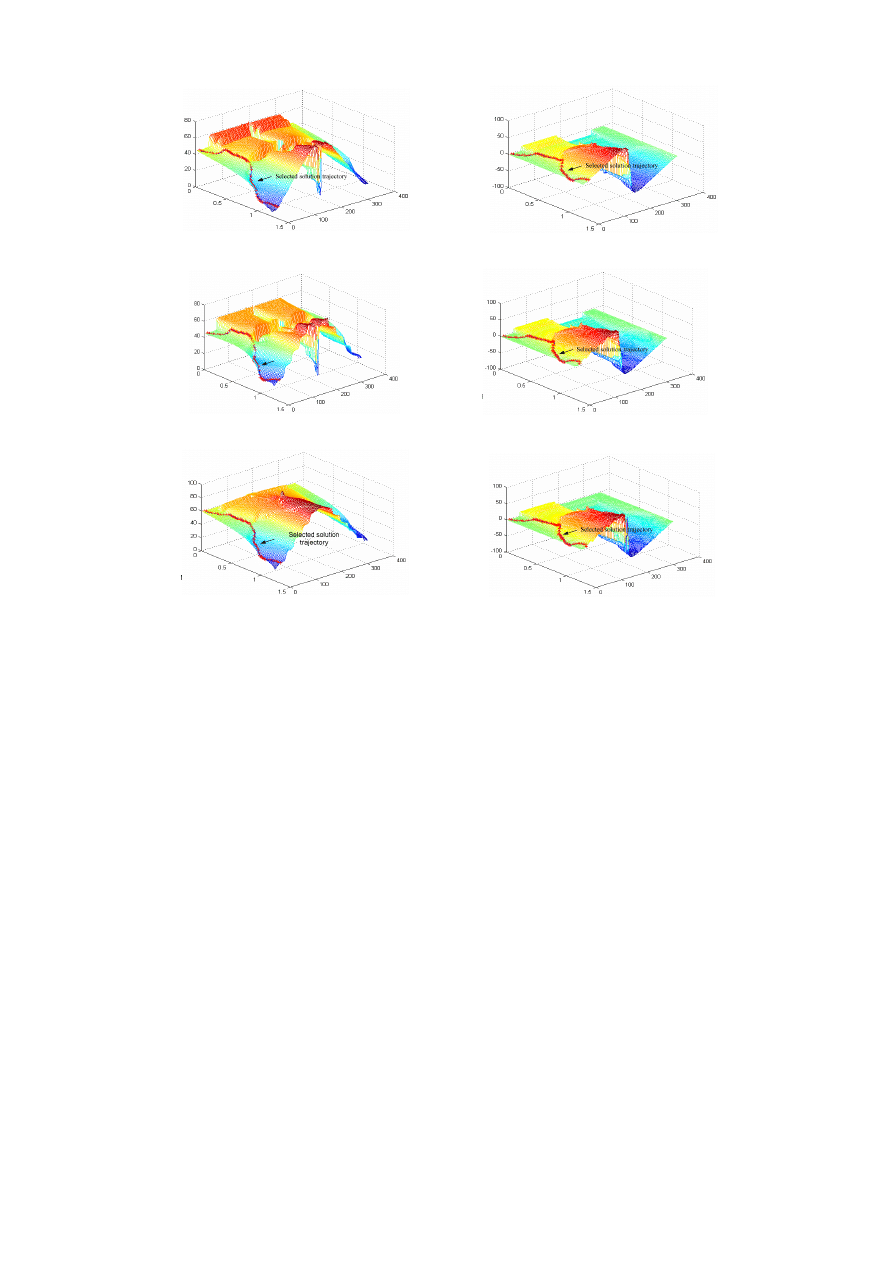
Fig. 5. 3-dimension graphs of the solution angles. (a)

1

α ,(b)

1

φ ,(c)

2

α ,(d)

2

φ (e)

3

α ,(f)

3

φ .

where

p

m is the magnitude and

p

γ

is the phase of the p th

harmonic in the set N . It should be noted that (4) and (5) are
constructed by a fixed square wave and k quasi-square waves.
When the harmonic phase

p

γ

varies, both

i

α

and

i

φ

are

variables but the square wave is still fixed. Equations (4) and
(5) imply a half-wave symmetry which guarantees that the
even harmonics will be zero. If there are k notch angles in the
period of first-half cycle, it will generate 2k variables
including k notch angles and k phase-shift angles. Thus it
brings k

controllable conditions. These k controllable

conditions result in 2 k equations, k real part equations and

k image part equations respectively. Being a nonlinear

equation set, it can be solved by some numerical solvers such
as Newton-Rephson method which provides faster
convergence speed. It should be note the solutions need to
meet the following conditions, otherwise they will be ignored.

1

2

0

90

i

α α

α

≤

≤

≤

≤

"

(8)

1

1

2

2

(

) (

)

(

)

i

i

α φ

α φ

α φ

+

≤

+

≤

+

"

(9)

1

1

1

1

(

) (

)

(

)

i

i

i

i

π α φ

π α

φ

π α φ

−

−

− +

≤

−

+

≤

−

+

"

(10)

In this paper, a SHE-PWM waveform with 3 notch angles

and 3 corresponding phase-shift angles are considered, and

controllable fundamental, zero 11-th harmonic and zero 13-th

harmonic are the three conditions. The equation set for problem

considered in this paper is given by (11). To satisfy these three

conditions described above, the amplitude modulation index

1

m is substituted by the desired fundamental magnitude, and

both

11

m and

13

m are set to zero. The last controllable factor

1

γ

is free to vary. It does not change the harmonic magnitude of

the controlled harmonics, but the uncontrolled harmonic
components will change with different

1

γ

. The next two lowest

order harmonics in this system are 23rd and 25th harmonics
that can be attenuated by choosing suitable

1

γ

. One set of

solutions at

1

m

=1 and

1

0

γ

= ° are

°

=

23

.

17

1

α

,

°

=

72

.

19

2

α

°

=

49

.

28

3

α

,

°

=

=

=

0

3

2

1

φ

φ

φ

.

Then,

1

γ

is incremented step by step and the solutions

obtained from the present step are used as initial value for the

next step. For the continuity of the solutions and to avoid

divergence, the incremental scale is two degrees. The solutions,

three notch angles and three corresponding phase-shift angles,

PEDS2009

390

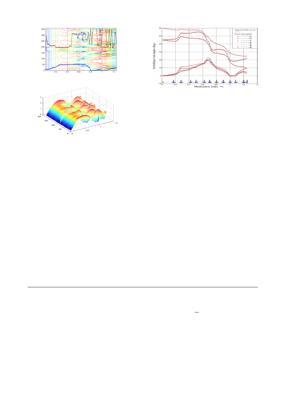
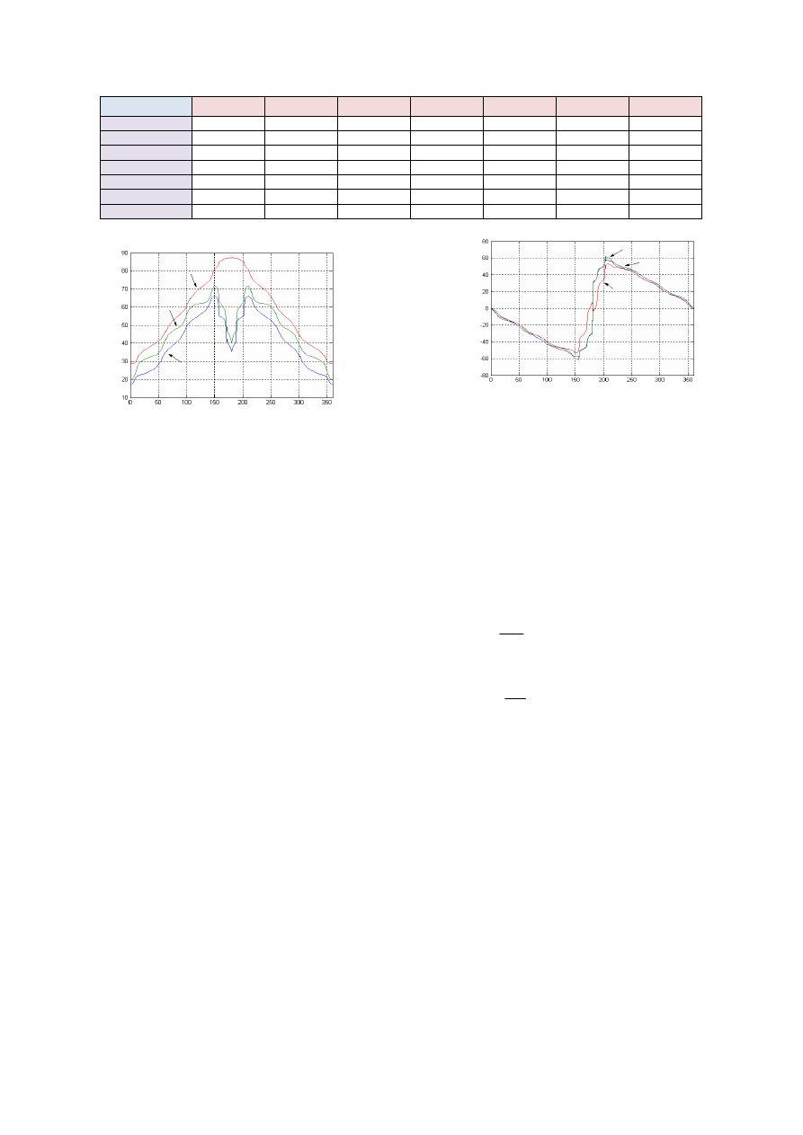
Fig. 7. The relationship between the exact data points and the appro-
ximated parabola segments.

1

m

1

(de

g.

)

γ

Route A

Route B

Modulation index

(a)

1

m

1

(deg .)

γ

23

,2

5

V

Modulation index

(b)

Fig. 6. (a) The contour of the rss value of 23rd and 25th harmonics, (b) 3-

D graph of the rss value of 23rd and 25th harmonics.

for

1

γ

varying from 0 to 360 degrees with fundamental

remaining unity are shown in Fig. 3 and Fig. 4.

It is worthy to mention that the solutions of

i

α

are

symmetric to the vertical line through 180 degrees and the
solutions of

i

φ

are symmetric to the point of

(

1

180

γ

=

° ,

0

i

φ

= ° ). These relationships simplify the

calculation work and only the first half range of

1

γ

needs to

deal with. These symmetric relationships are described in (12)

and (13).

(

)

(

)

i

i

α π ψ

α π ψ

+

=

+

(12)

(

)

(

)

i

i

φ π ψ

φ π ψ

+

= −

−

(13)

where the

ψ

can take any value from 0

° to 180° .

Next, the same processes are used to solve this problem at

different

1

m . Whenever the modulation index is increased or

decreased, the problem is solved by using the previous

solutions as initial values for the next step. After solving the
problem over the whole ranges of

1

m and

1

γ

, the solutions of 3

notch angles and 3 corresponding phase-shift angles can be

represented by 6 3-dimension graphs as shown in Fig.5. In each

3-dimension graph, x-axis and y-axis are denoted as

1

m and

1

γ

respectively, while z-axis is denoted as the solution angle.

According to the discussion on the previous section, the

harmonic distribution changes by varying the fundamental
phase

1

γ

. It can choose suitable solutions with respect to

1

γ

which minimizes 23rd and 25th harmonics. Therefore, the

root-sum-square values of 23rd and 25th harmonics, denoted
as

23,25

V

, contained in the output line-to-line voltage are

calculated over the full ranges of

1

m

and

1

γ

. Fig.6(a) shows

the contour map of the

23,25

V

and its 3-D diagram also shows

in Fig. 6(b). After searching the contour, the route with the
minimum

23,25

V

over the whole range of

1

m

is identified as

route A in Fig. 6(a). However route A is seriously tortuous and

is not suitable for on-line calculation by curve-fitting

approximation, which will be employed later in this paper.
Therefore, finding another routes with both relative-low

23,25

V

and acceptable smoothness is necessary. According to this

strategy, a smother route is chosen and marked as route B in
Fig. 6(a). Along route B, even its

23,25

V

is not the lowest, it

provides moderate smoothness so that on-line calculation based

on curve-fitting approximation can be implemented easily.

Once the route is decided, the solutions of notch angles

corresponding to the chosen route can also compose another

six routes which are shown in Fig. 5(a)-(f) by the marking
signs. The relationships between the solution angles and

1

m

corresponding to route B are shown in Fig. 7.

IV. O

N

-

LINE CALCULATION BASED ON

A

PPROXIMATED

P

OLYNOMIAL

D

ERIVED FROM

C

URVE

-F

ITTING

M

ETHOD

For avoiding burdened-on-line calculation, look-up table

derived from off-line calculated solutions is popular to

( )

1

1

2

2

2

2

1

1

2

2

2

2

1

1

2

2

2

2

1

1

2

2

3

3

1

2 cos

sin

2cos

sin

2cos

sin

2 cos11

sin11

2cos11

sin11

2cos11

sin11

2 cos13

sin13

2 cos13

sin13

2 cos13

sin13

,

1 2cos

cos

2cos

cos

2 cos

cos )

1 2cos11 cos1

F

α

φ

α

φ

α

φ

α

φ

α

φ

α

φ

α

φ

α

φ

α

φ

α φ

α

φ

α

φ

α

φ

α

−

×

+

×

−

×

−

×

+

×

−

×

−

×

+

×

−

×

=

− +

−

+

− +

( )

( )

( )

( )

( )

( )

1

1

11

11

13

13

1

1

1

2

2

3

3

11

11

1

1

2

2

3

3

13

13

cos

11

cos

13

cos

4

sin

1

2cos11

cos11

2 cos11

cos11

11

sin

1 2cos13 cos13

2 cos13

cos13

2 cos13

cos13

13

sin

m

m

m

m

m

m

γ

γ

γ

π

γ

φ

α

φ

α

φ

γ

α

φ

α

φ

α

φ

γ

⎡

⎤

⎡

⎤

⎢

⎥

⎢

⎥

×

⎢

⎥

⎢

⎥

⎢

⎥

⎢

⎥

×

⎢

⎥

=

⎢

⎥

⎢

⎥

⎢

⎥

⎢

⎥

⎢

⎥

−

+

⎢

⎥

×

⎢

⎥

⎢

⎥

⎢

⎥

− +

−

+

⎣

⎦

⎢

⎥

×

⎣

⎦

(11)

PEDS2009

391

implement SHE technique in many applications. However this

approach incurs mass memory occupancy and lacks flexibility.

Accessing the switching angles by approximated polynomials

using curve-fitting method is comparatively feasible [9]. In this

paper, the switching angles including their phase-shift angles

obtained from route B described in previous section are divided

into twelve segments as shown in the bottom of Fig. 7. Then,

the solutions of each angle in each segment are fitted by a

second-order polynomial obtained from least-square method,

and the coefficients of these parabolas are stored in the digital

controller. Constrained by the space, only the parabola
equations corresponding to range of

1

m

between 0.5 to 0.62,

which is one of the twelve segments, are given

(14)

37

.

35

75

.

134

41

.

84

)

(

68

.

9

72

.

51

46

.

19

)

(

73

.

29

08

.

147

33

.

120

)

(

49

.

63

65

.

462

55

.

441

)

(

59

.

79

58

.

503

39

.

470

)

(

40

.

11

55

.

139

62

.

137

)

(

1

2

1

1

3

1

2

1

1

2

1

2

1

1

1

1

2

1

1

3

1

2

1

1

2

1

2

1

1

1

⎪

⎪

⎪

⎪

⎭

⎪

⎪

⎪

⎪

⎬

⎫

−

+

−

=

−

+

−

=

−

+

−

=

−

+

−

=

−

+

−

=

+

−

−

=

m

m

m

m

m

m

m

m

m

m

m

m

m

m

m

m

m

m

φ

φ

φ

α

α

α

The number of segments and the orders of polynomials

are a compromise between accuracy of switching angle and
burden of calculation.

According to the desired amplitude

modulation index, the corresponding switching angles can be
calculated rapidly and precisely.

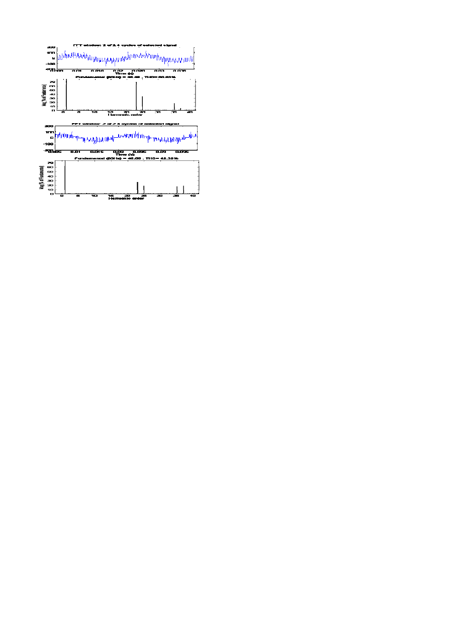
V.

E

XPERIMENTAL

R

ESULTS

According to the diagram shown in Fig. 1, a small-size

prototype is built to prove the validity of the proposed system.

In addition to the transformers, power stages and filter, a

digital-signal-processor chip (TMS320LF2812) is used to

implement the digital controller. Fig. 8 shows the waveforms
and spectrums of output line-to-line voltages with same

1

m but

with different

1

r

. In Fig. 8, the waveform with

1

r

=

°

50

and

1

m =0.5, which is a point of route B, has lower 23-rd and 25-th

harmonics than the waveform with

1

r

= 0

° and

1

m =0.5, which

is corresponding to quarter-wave-symmetry assumption. The

two lowest harmonics reduce from 69.78% and 35.61% to

27.62% and 19.39% respectively with next two higher order

harmonics slightly increasing. Moreover, the total harmonic

distortion reduces from 80.83% to 42.32% as well.

VI.

C

ONCLSION

This paper has proposed an SHE strategy with half-wave

symmetry assumption for use in a multi-level inverter system

cooperated with zig-zag connected transformers. Prohibited by

the transformers, only harmonics with orders 12n

±

1 appear in

the output line-to-line voltage. Therefore, SHE technology is

employed to handle these characteristic harmonics and a set of

three-notch-angle solutions, which eliminates 11-th and 13-th

harmonics, with full range of modulation index and

fundamental phase angle is obtained. A subset of solutions,

which is approximated by second-order polynomials for on-

line calculation, has been chosen to minimize 23-rd and 25-th

harmonics. Experimental results have shown the validity of the

proposed system.

R

EFERENCES

[1] H. S. and R. G. Hoft, “Generalized harmonic elimination and voltage

control in thyristor inverters: Part Ⅰ─harmonic elimination,” IEEE

Trans. Ind. Applicat., vol. IA-9, no. 3, PP. 310-317, May/Jun. 1973.

[2] ─, “Generalized harmonic elimination and voltage control in thyristor

inverters: Part Ⅱ ─ voltage control technique, ” IEEE Trans. Ind.

Applicat., vol. IA-10, no. 5, pp. 666-673, Sep/Oct. 1974.

[3] J. Sun, S. Btephan, and H. Grotstollen, “Optimal PWM Based on Real-

Time Solution of Harmonic Elimination Equations,” IEEE Trans. on

Power Electron., vol. 11, no. 4, pp. 612-621, July. 1996.

[4] J. R. Espinoza, G. Joos, J. I. Guzman, L. A. Moran, R. P. Burgos,”

Selective Harmonic Elimination and Current/Voltage Control in
Current/Voltage-Source Topologies: A Unified Approach,” IEEE Trans.

on Industrial Electronics, vol. 48, no. 1,pp. 71-81, February. 2001.

[5] V. G. Agelidis, A. I. Balouktsis, and M. S.A. Dahidah, “A Five-Level

Symmetrically Defined Selective Harmonic Elimination PWM Strategy:
Analysis and Experimental Validation,” IEEE Trans. Power Electron.,

vol. 23, no. 1, Jan., 2008.

[6] A. I. Maswood, “PWM SHE Switching Algorithm for Voltage Source

Inverter,” in Proc. IEEE Power Electron. Drive and Energy System

Conf., Dec. 2005, pp. 1–4.

[7] J. R. Wells, B. M. Nee, P. L. Chapman, and P. T. Krein, “Selective

harmonic control: A general problem formulation and selected
solutions,” IEEE Trans. Power Electron., vol. 20, no. 6, pp. 1337–1345,

Nov. 2005.

[8] Alireza Lhaligh, Jason R. Wells, Patrick L. Chapman, Philip T. Krein, “

Dead-Time Distortion in Generalized Selective Harmonic Control,”

IEEE Trans. Power Electron., vol. 23, no. 3, pp. 1511–1517, May. 2008.

[9] N. A. Azli, and A. H. Yatim, “Curve Fitting Technique for Optimal

Pulsewidth Modulation (PWM) Online Control of a Voltage Source

Inverter (VSI),” in proc. TENCON 2000, vol. 1, pp. 1337–1345, 2005.

(a)

(b)

Fig. 8. Waveforms and spectrums of line-to-line output voltages. (a)

°

= 0

1

r

and

5

.

0

1

=

m

. (b)

°

= 50

1

r

and

5

.

0

1

=

m

PEDS2009

392