
Acquisition of Malicious Code Using Active Learning
Robert Moskovitch
Deutche Telekom Laboratories at
Ben Gurion University
Beer Sheva 84105, Israel
robertmo@bgu.ac.il
Nir Nissim
Deutche Telekom Laboratories at
Ben Gurion University
Beer Sheva 84105, Israel
nirni@bgu.ac.il
Yuval Elovici
Deutche Telekom Laboratories at
Ben Gurion University
Beer Sheva 84105, Israel
elovici@bgu.ac.il
ABSTRACT
The recent growth in network usage has motivated the creation of
new malicious code for various purposes, including economic and
other malicious purposes. Currently, dozens of new malicious
codes are created every day, and this number is expected to
increase in coming years. Today’s signature-based anti-viruses
and heuristic-based methods are accurate, but cannot detect new
malicious code. Recently, classification algorithms were used
successfully for the detection of malicious code. We present a
complete methodology for the detection of unknown malicious
code, inspired by text categorization concepts. However, this
approach can be exploited further to achieve a more accurate and
efficient acquisition method of unknown malicious files. We use
an Active-Learning framework that enables the selection of the
unknown files for fast acquisition. We performed an extensive
evaluation of a test collection consisting of more than 30,000
files. We present a rigorous evaluation setup, consisting of real-
life scenarios, in which the malicious file content is expected to be
low, at about 10% of the files in the stream. We define specific
evaluation measures based on the known precision and recall
measures, which show the accuracy of the acquisition process and
the improvement in the classifier resulting from the efficient
acquisition process.
General Terms
Measurement, Performance, Experimentation, Security
Keywords
Malicious code detection, Active Learning.
1.
INTRODUCTION
The term malicious code (malcode) commonly refers to pieces of
code, not necessarily executable files, which are intended to harm,
generally or in particular, the specific owner of the host. Malcodes
are classified, based mainly on their transport mechanism, into
five main categories: worms, viruses, Trojans, and a new group
that is becoming more common, which comprises remote access
Trojans and backdoors. The recent growth in high-speed internet
connections and internet network services has led to an increase in
the creation of new malicious codes for various purposes, based
on economic, political, criminal or terrorist motives (among
others). Some of these codes have been used to gather
information, such as passwords and credit card numbers, as well
as for behavior monitoring. A recent survey by McAfee indicates
that about 4% of search results from the major search engines on
the web contain malicious code. Additionally, Shin et al. [17]
found that above 15% of the files in the KaZaA network
contained malicious code. Thus, we assume that the proportion of
malicious files in real life is about or less than 10%, but we also
consider other options.
Current anti-virus technology is primarily based on two
approaches. Signature-based methods, which rely on the
identification of unique strings in the binary code, while being
very precise, are useless against unknown malicious code. The
second approach involves heuristic-based methods, which are
based on rules defined by experts, which define a malicious
behavior, or a benign behavior, in order to enable the detection of
unknown malcodes [6]. Other proposed methods include behavior
blockers, which attempt to detect sequences of events in operating
systems, and integrity checkers, which periodically check for
changes in files and disks. However, besides the fact that these
methods can be bypassed by viruses, their main drawback is that,
by definition, they can only detect the presence of a malcode after
the infected program has been executed, unlike the signature-
based methods, including the heuristic-based methods, which are
very time-consuming and have a relatively high false alarm rate.
The generalization of the detection methods, so that unknown
malcodes can be detected, is therefore crucial. Recently,
classification algorithms were employed to automate and extend
the idea of heuristic-based methods. As we will describe in more
detail shortly, the binary code of a file is represented by n-grams,
and classifiers are applied to learn patterns in the code and
classify large amounts of data. A classifier is a rule set which is
learnt from a given training-set, including examples of classes,
both malicious and benign files in our case. Recent studies, which
we survey in the next section, have shown that this is a very
successful strategy.
Another problem which is troubling the anti virus community is
the acquisition of new malicious files, which it is very important
to detect as quickly as possible. This is often done by using
honey-pots. Another option is to scan the traffic at the internet
service provider, if accessible, to increase the probability of
detection of a new malcode. However, the main challenge in both
options is to scan all the files efficiently, especially when scanning
internet node (router) traffic.
We present a methodology for malcode categorization based on
concepts from text categorization. We present an extensive and
rigorous evaluation of many factors in the methodology, based on
Permission to make digital or hard copies of all or part of this
work for personal or classroom use is granted without fee
provided that copies are not made or distributed for profit or
commercial advantage and that copies bear this notice and the
full citation on the first page. To copy otherwise, or republish, to
post on servers or to redistribute to lists, requires prior specific
permission and/or a fee. PinKDD'08, August 24, 2008, Las
Vegas, Nevada, USA.Copyright 2008 ACM...$5.00.

SVM classifiers using three types of kernels. The evaluation is
based on a test collection containing more than 30,000 files. In
this study we focus on the problem of efficiently scanning and
acquiring new malicious code in a stream of executable files using
Active Learners. We start with a survey of previous relevant
studies. We describe the methods we used to represent the
executable files. We present our approach of acquiring new
malcodes using Active Learning and perform a rigorous
evaluation. Finally, we present our results and discuss them.
2.
BACKGROUND
2.1
Detecting Malcodes via Data Mining
Over the past five years, several studies have investigated the
option of detecting unknown malcode based on its binary code.
Schultz et al. [16] were the first to introduce the idea of applying
machine learning (ML) methods for the detection of different
malcodes based on their respective binary codes. They used three
different feature extraction (FE) approaches -- program header,
string features, and byte sequence features -- in which they
applied four classifiers -- a signature-based method (anti-virus),
Ripper, a rule-based learner, Naïve Bayes, and Multi-Naïve
Bayes. This study found that all the ML methods were more
accurate than the signature-based algorithm. The ML methods
were more than twice as accurate, with the out-performing method
being Naïve Bayes, using strings, or Multi-Naïve Bayes using
byte sequences. Abou-Assaleh et al. [1] introduced a framework
that used the common n-gram (CNG) method and the k nearest
neighbor (KNN) classifier for the detection of malcodes. For each
class, malicious and benign, a representative profile was
constructed and assigned a new executable file. This executable
file was compared with the profiles and matched to the most
similar. Two different datasets were used: the I-worm collection,
which consisted of 292 Windows internet worms, and the win32
collection, which consisted of 493 Windows viruses. The best
results were achieved using 3-6 n-grams and a profile of 500-5000
features. Kolter and Maloof [9] presented a collection that
included 1971 benign and 1651 malicious executables files. N-
grams were extracted and 500 were selected using the information
gain measure [12]. The vector of n-gram features was binary,
presenting the presence or absence of a feature in the file and
ignoring the frequency of feature appearances. In their
experiment, they trained several classifiers: IBK (KNN), a
similarity based classifier called TFIDF classifier, Naïve Bayes,
SVM (SMO), and Decision tree (J48), the last three of which
were also boosted. Two main experiments were conducted on two
different datasets, a small collection and a large collection. The
small collection consisted of 476 malicious and 561 benign
executables and the larger collection of 1651 malicious and 1971
benign executables. In both experiments, the four best-performing
classifiers were Boosted J48, SVM, boosted SVM, and IBK.
Boosted J48 out-performed the others, The authors indicated that
the results of their n-gram study were better than those presented
by Schultz and Eskin [16]. Recently, Kolter and Maloof [10]
reported an extension of their work, in which they classified
malcodes into families (classes) based on the functions in their
respective payloads. In the categorization task of multiple
classifications, the best results were achieved for the classes: mass
mailer, backdoor, and virus (no benign classes). In attempts to
estimate their ability to detect malicious codes based on their
issue dates, these classifiers were trained on files issued before
July 2003, and then tested on 291 files issued from that point in
time through August 2004. The results were, as expected, not as
good as those of previous experiments. These results indicate the
importance of maintaining such a training set through the
acquisition of new executables, in order to cope with unknown
new executables. Henchiri and Japkowicz [7] presented a
hierarchical feature selection approach which makes possible the
selection of n-gram features that appear at rates above a specified
threshold in a specific virus family, as well as in more than a
minimal amount of virus classes (families). They applied several
classifiers, ID3, J48 Naïve Bayes, SVM- and SMO, to the dataset
used by Schultz et al. [16] and obtained results that were better
than those obtained using a traditional feature selection, as
presented in [16], which focused mainly on 5-grams. However, it
is not clear whether these results are reflective more of the feature
selection method or of the number of features that were used.
Moskovitch et al [13], who are the authors of this study, presented
a test collection consisting of more than 30,000 executable files,
which is the largest known to us. They performed a wide
evaluation consisting of five types of classifiers and focused on
the imbalance problem in real life conditions, in which the
percentage of malicious files is less than 10%, based on recent
surveys. After evaluating the classifiers on varying percentages of
malicious files in the training set and test sets, it was shown to
achieve the optimal results when having similar proportions in the
training set as expected in the test set.
2.2
Active Learning and Selective Sampling
A major challenge in supervised learning is labeling the examples
in the dataset. Often the labeling is expensive since it is done
manually by human experts. Labeled examples are crucial in order
to train a classifier, and we would therefore like to reduce the
number of labeling requirements. The Active Learning (AL)
approach proposes a method which asks actively for labeling of
specific examples, based on their potential contribution to the
learning process. AL is roughly divided into two major
approaches: the membership queries [2] and the selective-
sampling approach [11]. In the membership queries approach the
learner constructs artificial examples from the problem space, then
asks for its label from the expert, and finally learns from it and so
forth, in an attempt to cover the problem space and to have a
minimal number of examples that represent most of the types
among the existing examples. However, a potential practical
problem in this approach is requesting a label for a nonsense
example. The selective-sampling approach usually comprises a
pool-based sampling, in which the learner is given a large set of
unlabeled data (pool) from which it iteratively selects the most
informative and contributive examples for labeling and learning,
based on which it is carefully selects the next examples, until it
meets stopping criteria.
Studies in several domains successfully applied active learning in
order to reduce the effort of labeling examples. Unlike in random
learning, in which a classifier is trained on a pool of labeled
examples, the classifier actively indicates the specific examples
that should be labeled, which are commonly the most informative
examples for the training task. Two AL methods were considered
in our experiments: Simple-Margin Tong and Koller [18] Error-
Reduction Roy and McCallum [14].

2.3
Acquisition of New Malicious Code Using
Active Learning
As we presented briefly earlier the option of acquiring new
malicious files from the web and internet services providers is
essential for fast detection and updating of the anti-viruses, as
well as updating of the classifiers. However, manually inspecting
each potentially malicious file is time-consuming, and often done
by human experts. We propose using Active Learning as a
selective sampling approach based on a static analysis of
malicious code, in which the active learner identifies new
examples which are expected to be unknown. Moreover, the
active learner is expected to present a ranked list of the most
informative examples, which are probably the most different from
what currently is known.
3.
METHODS
3.1
Text Categorization
To detect and acquire unknown malicious code, we suggest
implementing well-studied concepts from the information
retrieval (IR) and more specific text categorization domain. In
execution of our task, binary files (executables) are parsed and n-
gram terms are extracted. Each n-gram term in our task is
analogous to words in the textual domain. Here are descriptions of
the IR concepts used in this study. Salton and Weng [15]
presented the vector space model to represent a textual file as a
bag-of-words. After parsing the text and extracting the words, a
vocabulary of the entire collection of words is constructed. Each
of these words may appear zero to multiple times in a document.
A vector of terms is created, such that each index in the vector
represents the term frequency (TF) in the document. Equation 1
shows the definition of a normalized TF, in which the term
frequency is divided by the maximal appearing term in the
document with values in the range of [0-1]. Another common
representation is the TF Inverse Document Frequency (TFIDF),
which combines the frequency of a term in the document (TF) and
its frequency in the documents collection, as shown in Equation 2,
in which the term's (normalized) TF value is multiplied by the
IDF = log (N/n), where N is the number of documents in the
entire file collection and n is the number of documents in which
the term appears.
)
max(
document
in
frequency
term
frequency
term
TF
=
(1)
n
N
DF
where
DF
TF
TFIDF
=
=
),
log(
*
(2)
3.2
Data Set Creation
We created a dataset of malicious and benign executables for the
Windows operating system, which is the most commonly used and
attacked. To the best of our knowledge, this collection is the
largest ever assembled. We acquired the malicious files from the
VX Heaven website1, having 7688 malicious files. To identify the
1
http://vx.netlux.org
files, we used the Kaspersky2 anti-virus and the Windows version
of the Unix ‘file’ command for file type identification. The files in
the benign set, including executable and Dynamic Linked Library
(DLL) files, were gathered from machines running the Windows
XP operating system, which is currently considered the most used,
on our campus. The benign set contained 22,735 files, which were
reported by the Kaspersky anti-virus program as being completely
virus-free.
3.3
Data Preparation and Feature Selection
We parsed the binary code of the executable files using several n-
gram lengths moving windows, denoted by n. Vocabularies of
16,777,216, 1,084,793,035, 1,575,804,954 and 1,936,342,220, for
3-gram, 4-gram, 5-gram and 6-gram, respectively, were extracted.
Later the TF and TFIDF representation were calculated for each
n-gram in each file.
In machine learning applications, the large number of features
(many of which do not contribute to the accuracy and may even
decrease it) in many domains presents a huge problem. Moreover,
in our task a reduction in the amount of features is crucial for
practical reasons, but must be performed while simultaneously
maintaining a high level of accuracy. This is due to the fact that,
as shown earlier, the vocabulary size may exceed billions of
features, far more than can be processed by any feature selection
tool within a reasonable period of time. Additionally, it is
important to identify those terms that appear in most of the files,
in order to avoid zeroed representation vectors. Thus, initially the
features having the highest DF value (Equation 2) were extracted.
Based on the DF measure, two sets were selected, the top 5,500
terms and the top 1,000-6,500 terms. The set of top 1000 to 6,500
set of features was inspired by the removal of stop-words, as often
done in information retrieval for common words. Later, feature
selection methods were applied to each of these two sets. Since it
is not the focus of this paper, we will describe the feature
selection preprocessing very briefly. We used a filters approach,
in which the measure was independent of any classification
algorithm, to compare the performances of the different
classification algorithms. In a filters approach, a measure is used
to quantify the correlation of each feature to the class (malicious
or benign) and estimate its expected contribution to the
classification task. Three feature selection measures were used: as
a baseline we used the document frequency measure DF
(Equation 2), and additionally the Gain Ratio (GR) [12] and
Fisher Score [5]. Eventually the top 50, 100, 200 300, 1000, 1500
and 2000 were selected from each feature selection.
3.4
Support Vector Machines
We employed the SVM classification algorithm using three
different kernel functions, in a supervised learning approach. We
briefly introduce the SVM classification algorithm and the
principles and implementation of Active Learning that we used in
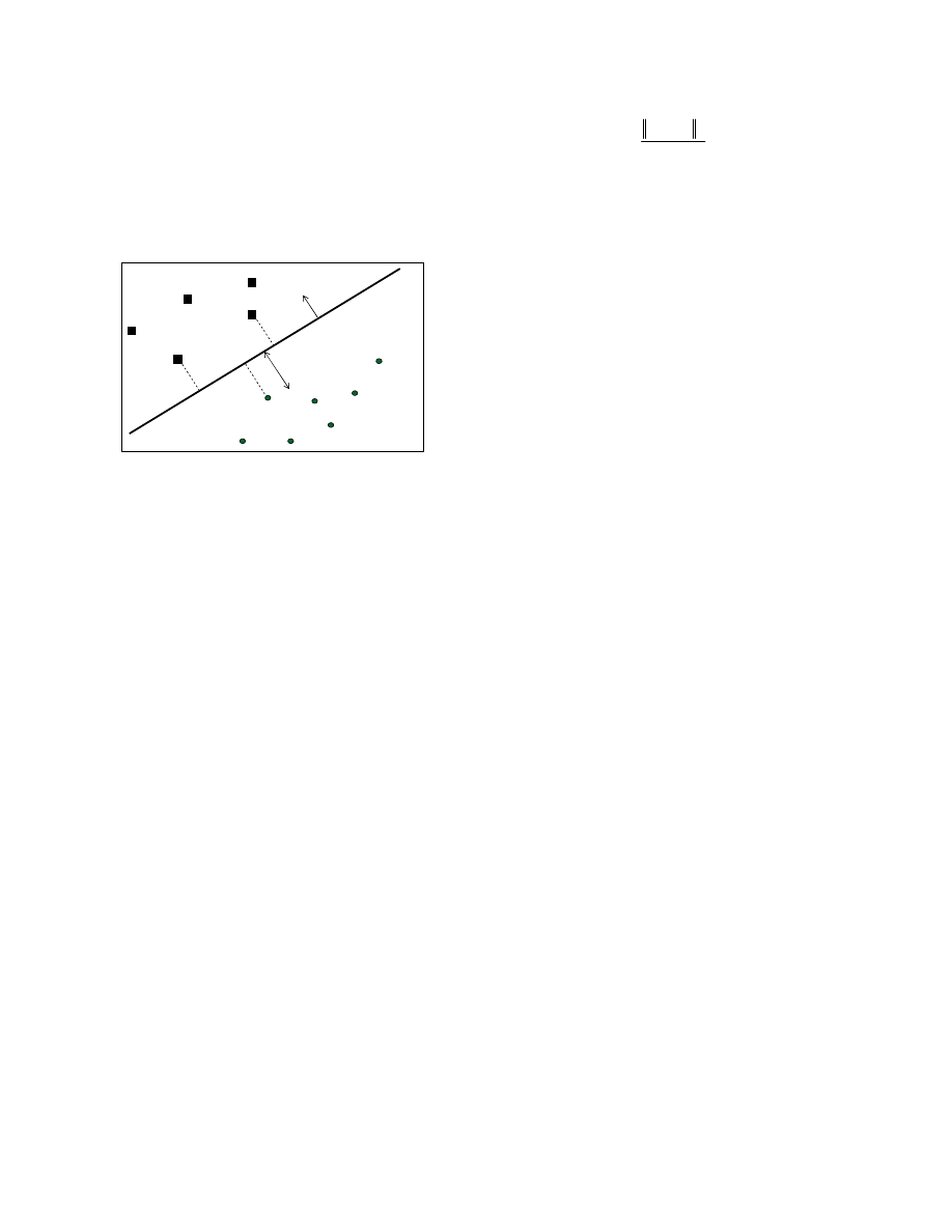
this study. SVM is a binary classifier which finds a linear
hyperplane that separates the given examples into the two given
classes. Later an extension that enables handling multiclass
classification was developed. SVM is widely known for its
capacity to handle a large amount of features, such as text, as was
shown by Joachims [8]. We used the Lib-SVM implementation of
Chang [4] that also handles multiclass classification. Given a
2
http://www.kaspersky.com
training set, in which an example is a vector x
i
= <f
1
,f
2
…f
m
>,
where f
i
'
is a feature, and labeled by yi = {-1,+1}, the SVM
attempts to specify a linear hyperplane that has the maximal
margin, defined by the maximal (perpendicular) distance between
the examples of the two classes. Figure 1 illustrates a two
dimensional space, in which the examples are located according to
their features and the hyperplane splits them according to their
label.
Class (+1)
Class(-1)
margin
W
Figure 1. An SVM that separates the training set into two classes,
having maximal margin in a two dimensional space.
The examples lying closest to the hyperplane are the "supporting
vectors" W, the Normal of the hyperplane, is a linear combination
of the most important examples (supporting vectors), multiplied
by LaGrange multipliers (alphas). Since the dataset in the original
space often cannot be linearly separated, a kernel function K is
used. SVM actually projects the examples into a higher
dimensional space in order to create linear separation of the
examples. Note that when the kernel function satisfies Mercer's
condition, as was explained by Burges [3], K can be written as
shown in Equation 3, where Φ is a function that maps the example
from the original feature space into a higher dimensional space,
while K relies on "inner product" between the mappings of
examples x
1
, x
2
. For the general case, the SVM classifier will be in
the form shown in Equation 4, while n is the number of examples
in training set, and w is defined in Equation 5.
)
(
)
(
)
,
(
2
1
2
1
x
x
x
x
Φ
⋅
Φ
=
K
(3)
(
)
=
Φ
⋅
=
∑
)
(
)
(
)
(
1
n
i
i
i
x
x
K
y
sign
x
w
sign
x
f
α
(4)
∑
Φ
=
n
i
i
i
x
y
w
1
)
(
α
(5)
Two commonly used kernel functions were used: Polynomial
kernel, as shown in Equation 6, creates polynomial values of
degree p, where the output depends on the direction of the two
vectors, examples x
1
, x
2
, in the original problem space. Note that a
private case of a polynomial kernel, having p=1, is actually the
Linear kernel. Radial Basis Function (RBF), as shown in Equation
7, in which a Gaussian is used as the RBF and the output of the
kernel depends on the Euclidean distance of examples x
1
, x
2
.
P
K
)
1
(
)
,
(
2
1
2
1
+
⋅
=
x
x
x
x
(6)
)
2
exp(
)
,
(
2
2
2
1
2
1
σ
x
x
x
x
−
−
=
K
(7)
3.5
Active Learning
In this study we implemented two selective sampling (pool-based)
AL methods: the Simple Margin presented by Tong and Koller,
[18] and Error Reduction presented by Roy and McCallum, [14].
3.5.1
Simple-Margin
This method is directly oriented to the SVM classifier. As was
explained in the section 3.4, by using a kernel function, the SVM
implicitly projects the training examples into a different (usually
higher dimensional) feature space, denoted by F. In this space
there is a set of hypotheses that are consistent with the training-
set, meaning that they create linear separation of the training-set.
This set of consistent hypotheses is called the Version-Space
(VS). From among the consistent hypotheses, the SVM then
identifies the best hypothesis that has the maximal margin. Thus,
the motivation of the Simple-Margin AL method is to select those
examples from the pool, so that these will reduce the number of
hypotheses in the VS, in an attempt to achieve a situation where
VS contains the most accurate and consistent hypotheses.
Calculating the VS is complex and impractical when large
datasets are considered, and therefore this method is oriented
through simple heuristics that are based on the relation between
the VS and the SVM with the maximal margin. Practically,
examples that lie closest to the separating hyperplane (inside the
margin) are more likely to be informative and new to the
classifier, and thus will be selected for labeling and acquisition.
3.5.2
Error-Reduction
The Error Reduction method is more general and can be applied
to any classifier that can provide probabilistic values for its
classification decision. Based on the estimation of the expected
error, which is achieved through adding an example into the
training-set with each label, the example that is expected to lead
to the minimal expected error will be selected and labeled. Since
the real future error rates are unknown, the learner utilizes its
current classifier in order to estimate those errors. In the
beginning
of
an
AL
trial,
an
initial
classifier
)
|
(
^
x
y
P
D
is trained over a randomly
selected initial set D. For every optional label y
∈
Y
(of every
example x in the pool P) the algorithm induces a new classifier
)
|
(
^
|
x
y
P
D
trained on the extended training set D' =
D
+ (x, y), Thus (in our binary case, malicious and benign are the
only optional labels) for every example X there are two classifiers,
each one for each label. Then for each one of the example's
classifiers the future expected generalization error is estimated
using a log-loss function, shown in Equation 8. The log-loss
function measures the error degree of the current classifier over all
the examples in the pool, where this classifier represents the
induced classifier as a result of selecting a specific example from
the pool and adding it to the training set, having a specific label.
Thus, for every example x
∈
P
we actually have two future
generalization errors (one for each optional label as was
calculated in Equation 8). Finally, an average is calculated for the
two errors, which is called the self-estimated average error, based
on Equation 9. It can be understood that it is built of the weighted
average so that the weight of each error of example x with label y
is given by the prior probability of the initial classifier to classify
correctly example x with label y. Finally, the example x with the
lowest expected self-estimated error is chosen and added to the
training set. In a nutshell, an example will be chosen from the
pool only if it dramatically improves the confidence of the current
classifier more than all the examples in the pool (means lower
estimated error).
∑ ∑
∈
∈
⋅
=
P
x
Y
y
D
D
P
x
y
P
x
y
P
P
E
D
))
|
(
log(
)
|
(
1
^
^
|
|
^
'
(8)
^
'
)
|
(
^
D
P
Y
y
D
E
x
y
P
⋅
∑
∈
(9)
4.
Evaluation
To evaluate the use of AL in the task of efficient acquisition of
new files, we defined specific measures derived from the
experimental objectives. The first experimental objective was to
determine the optimal settings of the term representation (TF or
TFIDF), n-grams representation (3, 4, 5 or 6), the best global
range (top 5500 or top 1000-6500) and feature selection method
(DF, FS or GR), and the top selection (50, 100, 200, 300, 1000,
1500 or 2000). After determining the optimal settings, we
performed a second experiment to evaluate our proposed
acquisition process using the two AL methods.
4.1
Evaluation Measures
For evaluation purposes, we measured the True Positive Rate
(TPR) measure, which is the number of positive instances
classified correctly, as shown in Equation 10, False Positive Rate
(FPR), which is the number of negative instances misclassified
Equation 10, and the Total Accuracy, which measures the number
of absolutely correctly classified instances, either positive or
negative, divided by the entire number of instances, shown in
Equation 11.
|
|
|
|
|
|
FN
TP
TP
TPR
+
=
;
|
|
|
|
|
|
TN
FP
FP
R
FP
+
=
(10)
|
|
|
|
|
|
|
|
|
|
|
|
FN
TN
FP
TP
TN
TP
Accuracy
Total
+
+
+
+
=
(11)
4.2
Evaluation Measures for the Acquisition
Process
In this study we wanted to evaluate the acquisition performance of
the Active-Learner from a stream of files presented by the test set,
containing benign and malicious executables, including new
(unknown) and not-new files. Actually, the task here is to evaluate
the capability of the module to acquire the new files in the test set,
which cannot be evaluated only by the common measures
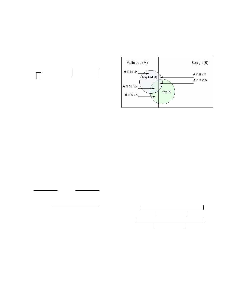
evaluated earlier. Figure 2 illustrates the evaluation scheme
describing the varying contents of the test set and Acquisition set
that will be explained shortly. The datasets contain two types of
files: Malicious (M) and Benign (B). While the Malicious region
is presented as a bit smaller, it is actually significantly smaller.
These datasets contain varying files partially known to the
classifier, from the training set, and a larger portion of New (N)
files, which are expected to be acquired by the Active Learner,
illustrated by a circle. The active learner acquires from the stream
part of the files, illustrated by the Acquired (A) circle. Ideally the
Acquired
circle will be identical to the New circle.
Figure 2. Illustration of the evaluation scheme, including the
Malicious (M) and Benign (B) Files, the New files to acquire (N)
and the actual Acquired (A) files.
To define the evaluation measures, we define the resultant regions
in the evaluation scheme by:
• A ∩ M \ N – The Malicious files Acquired, but not New.
• A ∩ M ∩ N – The Malicious files Acquired and New.
• M ∩ N \ A – The New Malicious files, but not Acquired.
• A ∩ B \ N – The Benign files Acquired, but not New.
• A ∩ B ∩ N – The Benign files Acquired and New.
For the evaluation of the said scheme we used the known
Precision and Recall measures, often used in information retrieval
and text categorization. We first define the traditional precision
and recall measures. Equation 12 represents the Precision, which
is the proportion of the accurately classified examples among the
classified examples. Equation 13 represents the Recall measure,
which is the proportion of the classified examples from a specific
class in the entire class examples.
{
} {
}
{
}
examples
classified
examples
classiifed
examples
relevant
precision
∩
=
(12)
{
} {
}
{
}
examples
relevant
documents
classified
examples
relevant
recall
∩
=
(13)
As we will elaborate later, the acquisition evaluation set will
contain both malicious and benign files, partially new (were not in
the training set) and partially not-new (appeared in the training
set), and thus unknown to the classifier. To evaluate the selective
method we define here the precision and recall measures in the
context of our problem. Corresponding to the evaluation scheme
presented in Figure 2, the precision_new_benign is defined in
Equation 14 by the proportion among the new benign files which
were acquired and the acquired benign files. Similarly the
precision_new_malicious is defined in Equation 15. The
recall_new_benign is defined in Equation 16 by how many new
benign files in the stream were acquired from the entire set of new
benign in the stream. The recall_new_malicious is defined
similarly in Equation 17.
B
A
N
B
A
Benign
new
precision
∩
∩
∩
=
_
_
(14)
M
A
N
M
A
Malicious
new
precision
∩
∩
∩
=
_
_
(15)
B
N
N
B
A
Benign
new
recall
∩
∩
∩
=
_
_
(16)
M
N
N
M
A
Malicious
new
recall
∩
∩
∩
=
_
_
(17)
The acquired examples are important for the incremental
improvement of the classifier; The Active Learner acquires the
new examples which are mostly important for the improvement of
the classifier, but not all the new examples are acquired,
especially these which the classifier is certain on their
classification. However, we would like to be aware of any new
files (especially malicious) in order to examine them and add
them to the repository. This set of files are the New and not
Acquired (N\A), thus, we would like to measure the accuracy of
the classification of these files to make sure that the classifier
classified them correctly. This is done using the Accuracy
measure as presented in Equation 11 on the subset defined by
(N\A), where for example |TP (N \ A)| is the number of malicious
executables that were labeled correctly as malicious, out of the
un-acquired new examples. In addition we measured the
classification accuracy of the classifier in classifying examples
which were not new and not acquired. Thus, using again the
Accuracy measure (Equation 11) for the ¬(N
∪
A) defines our
evaluation measure.
5.
Experiments and Results
5.1
Experiment 1
To determine the best settings of the file representation and the
feature selection we performed a wide and comprehensive set of
evaluation runs, including all the combinations of the optional
settings for each of the aspects, amounting to 1536 runs in a 5-
fold cross validation format for all the three kernels. Note that the
files in the test-set were not in the training-set presenting
unknown files to the classifier.
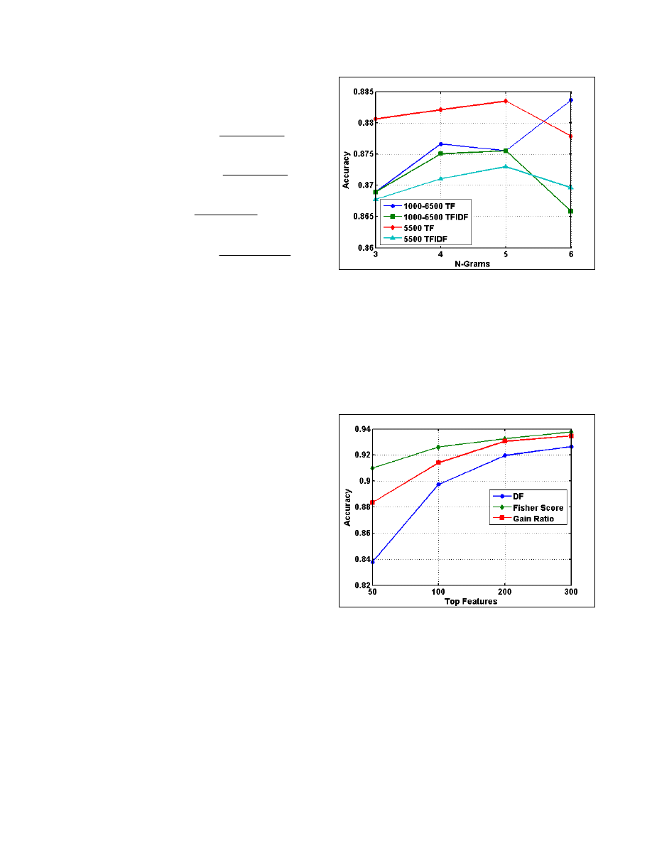
Global Feature Selection vs n-grams.
Figure 3 presents the mean
accuracy of the combinations of the term representations and n-
grams. The top 5,500 features outperformed with the TF
representation and the 5-gram in general. The out-performing of
the TF has meaningful computational advantages, on which we
will elaborate in the Discussion. In general, mostly the 5-grams
outperformed the others.
Figure 3. The results of the global selection, term representation,
and n-grams, in which the Top 5500 global selection having the
TF representation is outperforming, especially with 5-grams.
Feature Selections and Top Selections.
Figure 4 presents the
mean accuracy of the three feature selection methods and the
seven top selections. For fewer features, the FS outperforms,
while above the Top 300 there was not much difference.
However, in general the FS outperformed the other methods. For
all the three feature selection methods there is a decrease in the
accuracy when using above Top 1000 features.
Figure 4. The accuracy increased as more features were used,
while in general the FS outperformed the other measures.
Classifiers.
After determining the best configuration of 5-Grams,
Global top 5500, TF representation, Fischer score, and Top300,
we present in Table 1 the results of each SVM kernel. The RBF
kernel out-performed the others and had a low false positive rate,
while the other kernels also perform very well.

Table 1. The RBF kernel outperformed while maintaining a low
level of false positive.
Classifier
Accuracy
FP
FN
SVM-LIN
0.921
0.033
0.214
SVM-POL
0.852
0.014
0.544
SVM-RBF
0.939
0.029
0.154
5.2
Experiment 2: Files Acquisition
In the second experiment we used the optimal settings from
experiment 1, applying only the RBF kernel which outperformed
(Table 1). In this set of experiments, we set an imbalanced
representation of malicious-benign proportions in the test-set to
reflect real life conditions of 10% malicious files in the stream,
based on the information provided in the Introduction. In a
previous study [13] we found that the optimal proportions in such
scenario are similar settings in the training set. The Dataset
includes 25000 executables (22,500 benign, 2500 malicious),
having 10% malicious and: 90% benign contents as in real life
conditions.
The evaluation test collection included several components:
Training-Set, Acquisition-Set (Stream), and Test-set. The
Acquisition-set consisted of benign and malicious examples,
including known executables (that appeared in the training set)
and unknown executables (which did not appear in the training
set) and the Test-set included the entire Data-set.
These sets were used in the following steps of the experiment:
1. A Learner is trained on the Training-Set.
2. The model is tested on the Test-Set to measure the initial
accuracy.
3. A stream of files is introduced to the Active Learner, which
asks selectively for labeling of specific files, which are
acquired.
4. After acquiring all the new informative examples, the Learner
is trained on the new Training-Set.
5. The Learner is tested on the Test-Set.
We applied the learners in each step using 2 different variation of
cross validation for each AL method. For the Simple-Margin we
used variation of 10-fold cross validation. Thus, the Acquisition
Set (stream) contained part of the folds in the Training Set and the
Test Set, which was used for evaluation prior to the Acquisition
phase and after, contained all the folds.
5.2.1
Simple-Margin AL method
We applied the Simple Margin Active Learner in the experimental
setup presented earlier. Table 2 presents the mean results of the
cross validation experiment. Both the Benign and the Malicious
Precision were very high, above 99%, which means that most of
the acquired files were indeed new. The Recall measures were
quite low, especially the Benign Recall. This can be explained by
the need of the Active Learner to improve the accuracy. An
interesting fact is the difference in the Recall of the Malicious and
the Benign, which can be explained by the varying proportions in
the training set, which was 10% malicious.
The classification accuracy of the new examples that were not
acquired was very high as well, being close to 99%, which was
also the classification accuracy of the not new, which was 100%.
However, the improvement between the Initial and Final accuracy
was significant, which shows the importance and the efficiency in
the acquisition process.
Table 2: The Simple-Margin acquisition performance.
Measure
Simple Margin
Performance
Precision Benign
99.81%
Precision Malicious
99.22%
Recall Benign
33.63%
Recall Malicious
82.82%
)
\
(
A
N
Accuracy
98.90%
A)
(N ∪
¬
Accuracy
100%
Initial Accuracy on Test-Set
86.63%
Final Accuracy on Test-Set
92.13%
Number Examples in Stream
10250
Number of New Examples
7750
Number Examples Acquired
2931
5.2.2
Error-Reduction AL method
We performed the experiment using the Error Reduction method.
Table 3 presents the mean results of the cross validation
experiment. In the acquisition phase, the Benign Precision was
high, while the Malicious Precision was relatively low, which
means that almost 30% of the examples that were acquired were
not actually new. The Recall measures were similar to those for
the Simple-Margin, in which the Benign Recall was significantly
lower than the Malicious Recall. The classification accuracy of
the not acquired files was high both for the new and for the not
new examples.
Table 3: The Error-reduction acquisition performance.
Measure
Error Reduction
Performance
Precision Benign
97.563%
Precision Malicious
72.617%
Recall Benign
29.050%
Recall Malicious
75.676%
)
\
(
A
N
Accuracy
98.316%
A)
(N ∪
¬
Accuracy
100%
Initial Accuracy on Test-Set
85.803%
Final Accuracy on Test-Set
89.045%
Number Examples in Stream
3010
Number of New Examples
2016
Number Examples Acquired
761

6.
Discussion and Conclusions
We introduced the task of efficient acquisition of unknown
malicious files in a stream of executable files. We proposed using
Active Learning as a selective method for the acquisition of the
most important files in the stream to improve the classifier's
performance. This approach can be applied at a network
communication node (router) at a network service provider to
increase the probability of acquiring new malicious files. A
methodology for the representation of malicious and benign
executables for the task of unknown malicious code detection was
presented, adopting ideas from Text Categorization.
In the first experiment, we found that the TFIDF representation
has no added value over the TF, which is not the case in IR. This
is very important, since using the TFIDF representation introduces
some computational challenges in the maintenance of the
measurements whenever the collection is updated. To reduce the
number of n-gram features, which ranges from millions to
billions, we used the DF threshold. We examined the concept of
stop-words in IR in our domain and found that the top features
have to be taken (e.g., top 5500 in our case), and not those of an
intermediate level. Having the top features enables vectors which
are less zeroed, since the selected features appear in most of the
files. The Fisher Score feature selection outperformed the other
methods, and using the top 300 features resulted in the best
performance.
In the second experiment, we evaluated the proposed method of
applying Active Learning for the acquisition of new malicious
files. We examined two AL methods, Simple Margin and Error
Reduction, and evaluated them rigorously using cross validation.
The evaluation consisted of three main phases: training on the
initial Training-set and testing on a Test-set, acquisition phase on
a dataset including known files (which were presented in the
training set) and new files, and eventually evaluating the classifier
after the acquisition on the Test-set to demonstrate the
improvement in the classifier performance. For the acquisition
phase evaluation we presented a set of measures based on the
Precision and Recall measures dedicated for the said task, which
refer to each portion of the dataset, the acquired benign and
malicious, separately. For the not acquired files we evaluated the
performance of the classifier in classifying them accurately to
justify that indeed they did not need to be acquired.
In general, both methods performed very well, with the Simple
Margin performing better than the Error Reduction. In the
acquisition phase, the benign and malicious Precision was often
very high; however, the malicious Precision for the Error
Reduction was relatively low. The benign and malicious Recalls
were relatively low and reflected the classifier's needs. An
interesting phenomenon was that a significantly higher percentage
of new malicious files, relatively to the benign files, were
acquired. This can be explained by the imbalanced proportions of
the malicious-benign files in the initial training set. The
classification accuracy of the not acquired files, unknown and
known, was extremely high in both experimental methods.
The evaluation of the classifier before the acquisition (initial
training set) and after showed an improvement in accuracy which
justifies the process. However, the relatively low accuracy, unlike
in the first experiment, can be explained by the small training set
which resulted from the cross validation setup.
When applying such a method for practical purposes we propose
that a human first examine the malicious acquired examples.
However, note that there might be unknown files which were not
acquired, since the classifier didn’t consider them as informative
enough and often had a good level of classification accuracy.
However, these files should be acquired. In order to identify these
files, one can apply an anti-virus on the files which were not
acquired and were classified as malicious. The files which were
not recognized by the anti-virus are suspected as unknown
malicious files and should be examined and acquired.
ACKNOWLEDGMENTS
We would like to thank Clint Feher, who created the dataset and
Yuval Fledel for meaningful discussions and comments in the
efficient implementation aspects.
7.
REFERENCES
[1] Abou-Assaleh, T., Cercone, N., Keselj, V., and Sweidan, R.
(2004) N-gram Based Detection of New Malicious Code, in
Proceedings of the 28th Annual International Computer
Software and Applications Conference (COMPSAC'04)
.
[2] Angluin, D. (1988) Queries and concept learning. Machine
Learning, 2, 319-342.
[3] Burges, C. J.C. (1988) A tutorial on support vector
machines for pattern recognition. Data Mining and
Knowledge Discovery, 2:121–167.
[4] Chang, C. C. and Lin, C.-J. (2001) LIBSVM: a library for
support
vector
machines.
Software
available
at
http://www.csie.ntu.edu.tw/˜cjlin/libsvm.
[5] Golub, T., Slonim, D., Tamaya, P., Huard, C., Gaasenbeek,
M., Mesirov, J., Coller, H., Loh, M., Downing, J., Caligiuri,
M., Bloomfield, C., and E. Lander, E. (1999) Molecular
classification of cancer: Class discovery and class prediction
by gene expression monitoring, Science, 286:531-537.
[6] Gryaznov, D. Scanners of the Year 2000: Heuristics,
Proceedings of the 5th International Virus Bulletin, 1999
[7] Henchiri, O. and Japkowicz, N., A Feature Selection and
Evaluation Scheme for Computer Virus Detection.
Proceedings of ICDM-2006: 891-895, Hong Kong, 2006.
[8] Joachims, T. (1998-1). Making large-scale support vector
machine learning practical. In B. Sch¨olkopf, C. Burges, A.
S., editor, Advances in Kernel Methods: Support Vector
Machines. MIT Press, Cambridge, MA.
[9] Kolter, J.Z. and Maloof, M.A. (2004) Learning to detect
malicious executables in the wild, in Proceedings of the
Tenth ACM SIGKDD International Conference on
Knowledge Discovery and Data Mining, 470–478. New
York, NY: ACM Press.
[10] Kolter J., and Maloof M. (2006) Learning to Detect and
Classify Malicious Executables in the Wild, Journal of
Machine Learning Research 7 2721-2744.
[11] Lewis, D. and Gale, W. (1994) A sequential algorithm for
training text classifiers. In Proceedingsof the Seventeenth
Annual International ACM-SIGIR Conference on Research
and Development in Information Retrieval, pages 3–12.
Springer-Verlag.

[12] Mitchell T. (1997) Machine Learning, McGraw-Hill.
[13]
Moskovitch R, Stopel D, Feher C, Nissim N and Elovici
Y,(2008)
Unknown
Malcode
Detection
via
Text
Categorization
and
the
Imbalance
Problem,
IEEE
Intelligence and Security Informatics (ISI08), Taiwan, 2008.
[14]
Roy, N. and McCallum, A. (2001) Toward Optimal
Active Learning through Sampling Estimation of Error
Reduction, ICML 2001.
[15] Salton, G., Wong, A., and Yang, C.S. (1975) A vector space
model for automatic indexing. Communications of the ACM,
18:613-620.
[16] Schultz, M., Eskin, E., Zadok, E., and Stolfo, S. (2001) Data
mining methods for detection of new malicious executables,
in Proceedings of the IEEE Symposium on Security and
Privacy, 2001, pp. 178-184.
[17] Shin, S. Jung, J., Balakrishnan, H. (2006) Malware
Prevalence in the KaZaA File-Sharing Network, Internet
Measurement Conference (IMC)
, Brazil, October
[18]
Tong, S. and Koller, D. (2000) Support vector machine
active learning with applications to text classification.
Journal of Machine Learning Research, 2:45–66, 2000-
2001.
Wyszukiwarka
Podobne podstrony:
Detection of New Malicious Code Using N grams Signatures
Static Detection of Malicious Code in Executable Programs
Dynamic analysis of malicious code
N gram based Detection of New Malicious Code
Using Markov Chains to Filter Machine morphed Variants of Malicious Programs
Faster parameter detection of polymorphic viral binary code using hot list strategy
Application of Data Mining based Malicious Code Detection Techniques for Detecting new Spyware
Static Analysis of Binary Code to Isolate Malicious Behaviors
Parallel analysis of polymorphic viral code using automated deduction system
Detection of Injected, Dynamically Generated, and Obfuscated Malicious Code
WIRELESS CHARGING OF MOBILE PHONES USING MICROWAVES
78 1101 1109 Industrial Production of Tool Steels Using Spray Forming Technology
63 907 917 Chemical Depth Profiling of Tool Materials Using Glow Discharge Optical Emission
The Acquisition of the English Verb
Assessment of Borderline Pathology Using the Inventory of Interpersonal Problems Circumplex Scales (
Age and the Acquisition of English As a Foreign Language
A study of assessors performance using graphical methods
In vitro corrosion resistance of titanium made using differe
Acquisition of Languages Infant and Adult Data
więcej podobnych podstron