Kevin Campbell, University of Stirling, November 2005
1
1
2008
KOSZT I STRUKTURA
KAPITAŁU
Kevin Campbell, University of Stirling, November 2005
2
2
Cost of Capital
Cost of Capital - The return the firm’s
investors could expect to earn if they
invested in securities with comparable
degrees of risk
Capital Structure - The firm’s mix of
long term financing and equity financing

Kevin Campbell, University of Stirling, November 2005
3
3
Cost of Capital
The cost of capital represents the overall cost
of financing to the firm
The cost of capital is normally the relevant
discount rate to use in analyzing an
investment
The overall cost of capital is a weighted
average of the various sources:
•
WACC = Weighted Average Cost of Capital
•
WACC = After-tax cost x weights

Kevin Campbell, University of Stirling, November 2005
4
4
Cost of Debt
The cost of debt to the firm is the effective yield
to maturity (or interest rate) paid to its
bondholders
Since interest is tax deductible to the firm, the
actual cost of debt is less than the yield to
maturity:
•
After-tax cost of debt = yield x (1 - tax rate)
The cost of debt should also be adjusted for
flotation costs (associated with issuing new
bonds)
Kevin Campbell, University of Stirling, November 2005
5
5
with stock
with debt
EBIT
400,000
400,000
- interest expense
0
(50,000)
EBT
400,000
350,000
- taxes (34%)
(136,000) (119,000)
EAT 264,000
231,000
Example: Tax effects of
Example: Tax effects of
financing with debt
financing with debt
Now, suppose the firm pays $50,000 in
dividends to the shareholders
Kevin Campbell, University of Stirling, November 2005
6
6
with stock
with debt
EBIT
400,000
400,000
- interest expense
0
(50,000)
EBT
400,000
350,000
- taxes (34%)
(136,000) (119,000)
EAT 264,000
231,000
- dividends (50,000)
0
Retained earnings
214,000
231,000
Example: Tax effects of
Example: Tax effects of
financing with debt
financing with debt
Kevin Campbell, University of Stirling, November 2005
7
7
After-tax cost Before-tax cost Tax
of Debt of Debt
Savings
33,000 = 50,000 -
17,000
OR
33,000 = 50,000 ( 1 - .34)
Or, if we want to look at percentage costs:
-
=
Cost of Debt
Kevin Campbell, University of Stirling, November 2005
8
8
After-tax Before-tax
Marginal
% cost of % cost of x tax
Debt Debt rate
Kd = kd (1 - T)
.066 = .10 (1 - .34)
-
=
1
1
Cost of Debt

Kevin Campbell, University of Stirling, November 2005
9
9
Prescott Corporation issues a
$1,000
par,
20 year
bond paying the market
rate of
10%.
Coupons are annual.
The bond will sell for par since it pays
the market rate, but flotation costs
amount to
$50
per bond.
What is the pre-tax and after-tax cost
of debt for Prescott Corporation?
EXAMPLE: Cost of Debt
Kevin Campbell, University of Stirling, November 2005
10
10
Pre-tax cost of debt:
950 = 100(PVIFA 20, K
d
) +
1000(PVIF 20, K
d
)
using a financial calculator:
K
d
= 10.61%
After-tax cost of debt:
K
d
= K
d
(1 - T)
K
d
= .1061 (1 - .34)
K
d
= .07 = 7%
EXAMPLE: Cost of Debt
So a 10% bond
costs the firm
only 7%
(with flotation costs)
because interest
is tax deductible
Kevin Campbell, University of Stirling, November 2005
11
11
Cost of New Preferred Stock
Preferred stock:
•
has a fixed dividend (similar to debt)
•
has no maturity date
•
dividends are not tax deductible and are
expected to be perpetual or infinite
Cost of preferred stock = dividend
price -
flotation cost
Kevin Campbell, University of Stirling, November 2005
12
12
Cost of Preferred stock:
Example
Baker Corporation has preferred stock that sells for $100 per share and pays an annual
dividend of $10.50. If the flotation costs are $4 per share, what is the cost of new
preferred stock?
10.94%
.1094
4
-
$100
$10.50
K
P

Kevin Campbell, University of Stirling, November 2005
13
13
Cost of Equity:
Retained Earnings
Why is there a cost for retained
earnings?
Earnings can be reinvested or paid out
as dividends
Investors could buy other securities,
and earn a return.
Thus, there is an opportunity cost if
earnings are retained

Kevin Campbell, University of Stirling, November 2005
14
14
Cost of Equity:
Retained Earnings
Common stock equity is available through
retained earnings (R/E) or by issuing new
common stock:
•
Common equity = R/E + New common
stock
Kevin Campbell, University of Stirling, November 2005
15
15
Cost of Equity:
New Common Stock
The cost of new common stock is
higher than the cost of retained
earnings because of flotation costs
•
selling and distribution costs
(such as sales commissions) for
the new securities

Kevin Campbell, University of Stirling, November 2005
16
16
Cost of Equity
There are a number of methods
used to determine the cost of
equity
We will focus on two
Dividend growth Model
CAPM
Kevin Campbell, University of Stirling, November 2005
17
17
The Dividend Growth Model
Approach
Estimating the cost of equity: the dividend growth
model approach
According to the constant growth (Gordon) model,
D
1
P
0
=
R
E
- g
Rearranging D
1
R
E
= + g
P
0
Kevin Campbell, University of Stirling, November 2005
18
18
Example: Estimating the Dividend
Growth Rate
Percentage
Year Dividend Dollar Change Change
1990 $4.00-
-
1991
4.40$0.40 10.00%
1992
4.750.35
7.95
1993
5.250.50
10.53
1994
5.650.40
7.62
Average Growth Rate
(10.00 + 7.95 + 10.53 + 7.62)/4 = 9.025%

Kevin Campbell, University of Stirling, November 2005
19
19
Dividend Growth Model
This model has drawbacks:
Some firms concentrate on growth and do
not pay dividends at all, or only irregularly
Growth rates may also be hard to estimate
Also this model doesn’t adjust for market
risk
Therefore many financial managers prefer
the capital asset pricing model (CAPM) - or
security market line (SML) - approach for
estimating the cost of equity
Kevin Campbell, University of Stirling, November 2005
20
20
Capital Asset Pricing Model
(CAPM)
)
(
f
m
f
R
R
β
R
kj
Cost of
capital Risk-free
return
Average rate of return
on common stocks
(WIG)
Co-variance
of returns against
the portfolio
(departure from the average)
B < 1, security is safer than WIG average
B > 1, security is riskier than WIG average
Kevin Campbell, University of Stirling, November 2005
21
21
The Security Market Line (SML)
Required rate
of return
Percent
0.5
1.0
1.5
2.0
SML = R
f
+ (K
m
– R
f
)
Beta
(risk)
Market risk premium
20.
0
18.
0
16.
0
14.
0
12.
0
10.
0
8.0
5.5
R
f

Kevin Campbell, University of Stirling, November 2005
22
22
Finding the Required Return on Common
Stock using the Capital Asset Pricing
Model
The Capital Asset Pricing Model (CAPM) can be used to estimate the
required return on individual stocks. The formula:
R
K
R
K
f
m
j
f
j
where
j
K
= Required return on stock j
f
R
=
Risk-
free rate of return (usually current rate on Treasury Bill).
j
= Beta coefficient for stock j
represents risk of the stock
m
K =
Return in market as measured by some proxy portfolio (index)
Suppose that Ba
ker has the following values:
f
R
=
5.5%
j
=
1.0
m
K =
12%
.

Kevin Campbell, University of Stirling, November 2005
23
23
Finding the Required Return on Common
Stock using the Capital Asset Pricing
Model
Then, using the CAPM we would get a required
return of
12%
5.5
-
12
1.0
5.5
K
j
.

Kevin Campbell, University of Stirling, November 2005
24
24
CAPM/SML approach
Advantage: Evaluates risk, applicable
to firms that don’t pay dividends
Disadvantage: Need to estimate
•
Beta
•
the risk premium (usually based on past
data, not future projections)
•
use an appropriate risk free rate of interest
Kevin Campbell, University of Stirling, November 2005
25
25
Estimation of Beta: Measuring
Market Risk
Market Portfolio - Portfolio of all assets
in the economy
In practice a broad stock market
index, such as the WIG, is used to
represent the market
Beta - sensitivity of a stock’s return to
the return on the market portfolio
Kevin Campbell, University of Stirling, November 2005
26
26
Estimation of Beta
Theoretically, the calculation of beta is
straightforward:
Problems
1.
Betas may vary over time.
2.
The sample size may be inadequate.
3.
Betas are influenced by changing financial leverage and business risk.
Solutions
•
Problems 1 and 2 (above) can be moderated by more sophisticated
statistical techniques.
•
Problem 3 can be lessened by adjusting for changes in business and
financial risk.
•
Look at average beta estimates of comparable firms in the industry.
2
)
(
)
,
(
M
iM
M
M
i
σ
σ
R
Var
R
R
Cov
β

Kevin Campbell, University of Stirling, November 2005
27
27
Stability of Beta
Most analysts argue that betas are
generally stable for firms remaining in
the same industry
That’s not to say that a firm’s beta can’t
change
•
Changes in product line
•
Changes in technology
•
Deregulation
•
Changes in financial leverage

Kevin Campbell, University of Stirling, November 2005
28
28
What is the appropriate risk-
free rate?
Use the yield on a long-term bond if you are
analyzing cash flows from a long-term investment
For short-term investments, it is entirely
appropriate to use the yield on short-term
government securities
Use the nominal risk-free rate if you discount
nominal cash flows and real risk-free rate if you
discount real cash flows
Kevin Campbell, University of Stirling, November 2005
29
29
Survey evidence: What do you
use for the risk-free rate?
Corporations
Financial Advisors
90-day T-bill (4%)
90-day T-bill (10%)
3-7 year Treasuries (7%)
5-10 year Treasuries (10%)
10-year Treasuries (33%)
10-30 year Treasuries (30%)
20-year Treasuries (4%)
30-year Treasuries (40%)
10-30 year Treasuries (33%)
N/A (10%)
10-years or 90-day; depends
(4%)
N/A (15%)
Source: Bruner et. al. (1998)

Kevin Campbell, University of Stirling, November 2005
30
30
Weighted Average Cost of Capital
(WACC)
WACC weights the cost of equity and the
cost of debt by the percentage of each
used in a firm’s capital structure
WACC=(E/ V) x R
E
+ (D/ V) x R
D
x (1-T
C
)
•
(E/V)= Equity % of total value
•
(D/V)=Debt % of total value
•
(1-Tc)=After-tax % or reciprocal of corp tax rate
Tc. The after-tax rate must be considered
because interest on corporate debt is deductible

Kevin Campbell, University of Stirling, November 2005
31
31
WACC Illustration
ABC Corp has 1.4 million shares common valued at
$20 per share =$28 million. Debt has face value of
$5 million and trades at 93% of face ($4.65 million)
in the market. Total market value of both equity +
debt thus =$32.65 million. Equity % = .8576 and
Debt % = .1424
Risk free rate is 4%, risk premium=7% and ABC’s
β=.74
Return on equity per SML : R
E
= 4% + (7% x .
74)=9.18%
Tax rate is 40%
Current yield on market debt is 11%

Kevin Campbell, University of Stirling, November 2005
32
32
WACC Illustration
WACC = (E/V) x R
E
+ (D/V) x R
D
x (1-Tc)
= .8576 x .0918 + (.1424 x .11 x .60)
= .088126 or 8.81%

Kevin Campbell, University of Stirling, November 2005
33
33
Final notes on WACC
WACC should be based on market rates and
valuation, not on book values of debt or
equity
Book values may not reflect the current
marketplace
WACC will reflect what a firm needs to earn
on a new investment. But the new
investment should also reflect a risk level
similar to the firm’s Beta used to calculate
the firm’s R
E
.
•
In the case of ABC Co., the relatively low WACC of
8.81% reflects ABC’s β=.74. A riskier investment
should reflect a higher interest rate.

Kevin Campbell, University of Stirling, November 2005
34
34
Final notes on WACC
The WACC is not constant
It changes in accordance with the
risk of the company and with the
floatation costs of new capital
Kevin Campbell, University of Stirling, November 2005
35
35
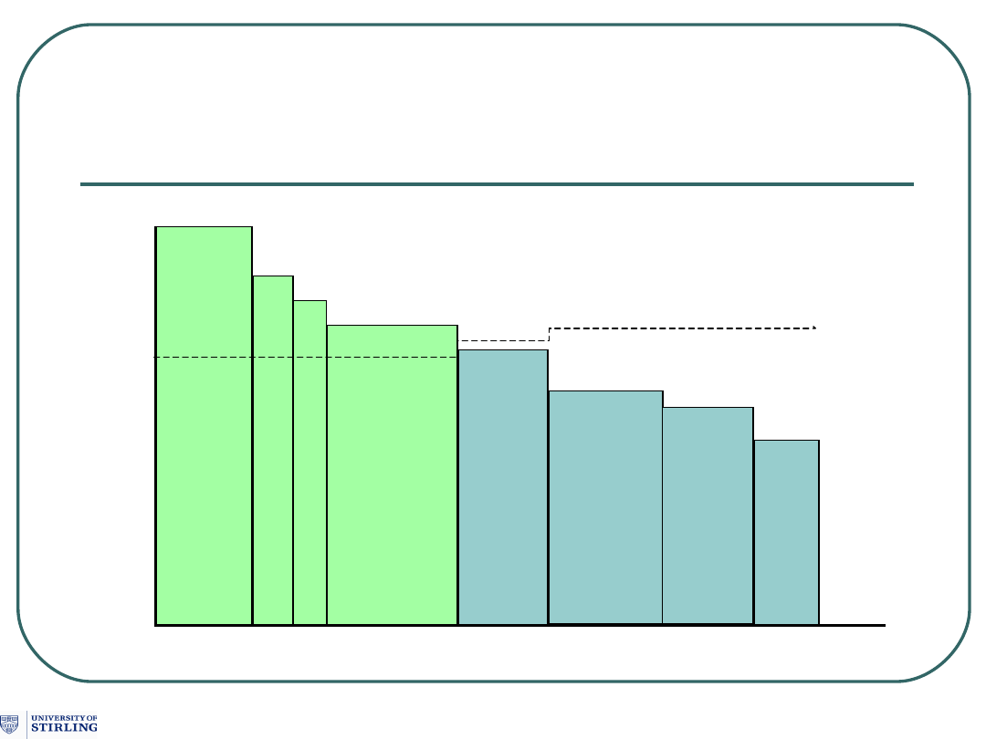
Marginal cost of capital and
investment projects
16.0
14.0
12.0
10.0
8.0
6.0
4.0
2.0
0.0
Percen
t
10 15
19
50
39
Amount of capital ($
millions)
11.23
%
70
85
95
Margin
al cost
of
capital
K
mc
A
B
C
D
E
F
G
H
10.77
%
10.41
%
-
-
-
-
-
-
-
-
-

Kevin Campbell, University of Stirling, November 2005
36
36
The End ….
KAPITAŁ - bogactwo zebrane uprzednio w celu podjęcia dalszej produkcji
(F. Quesnay, XVIII)
wszelki wynik procesu produkcyjnego, który przeznaczony jest do
późniejszego wykorzystania w procesie produkcyjnym (MCKenzzie,
Nardelli,1991)
całokształt zaangażowanych w przedsiębiorstwie wewnętrznych i
zewnętrznych, własnych i obcych, terminowych i nieterminowych
zasobów (bilans)
STRUKTURA KAPITAŁU
proporcja udziału kapitału własnego i obcego w finansowaniu działalności
przedsiębiorstwa
relacja wartości zadłużenia długoterminowego do kapitałów własnych
przedsiębiorstwa
struktura finansowania – struktura kapitału = zobowiązania
bieżące
ramy statycznego kompromisu, w którym przedsiębiorstwo ustala
docelową wielkość wskaźnika zadłużenia i stopniowo zbliża się do jego
osiągnięcia.
Document Outline
- Slide 1
- Slide 2
- Slide 3
- Slide 4
- Slide 5
- Slide 6
- Slide 7
- Slide 8
- Slide 9
- Slide 10
- Slide 11
- Slide 12
- Slide 13
- Slide 14
- Slide 15
- Slide 16
- Slide 17
- Slide 18
- Slide 19
- Slide 20
- Slide 21
- Slide 22
- Slide 23
- Slide 24
- Slide 25
- Slide 26
- Slide 27
- Slide 28
- Slide 29
- Slide 30
- Slide 31
- Slide 32
- Slide 33
- Slide 34
- Slide 35
- Slide 36
Wyszukiwarka
Podobne podstrony:
195 KC Cost of capital lecture kisk 2id 18506 ppt
196 Capital structure Intro lecture 1id 18514 ppt
12 Intro to origins of lg LECTURE2014
197 Capital structure lecture Gdansk 2006 Lecture 2id 18521 ppt
DV8 Physical Theatre the cost of living, STUDIA Pedagogika resocjalizacyjna
196 Capital structure Intro lecture 1id 18514 ppt
12 Intro to origins of lg LECTURE2014
Cost of living London
Max Weber Protestantism and The Spirit of Capitalism
[Форекс] The Cost of Technical Trading Rules in the Forex Market
w sapx363 Managing the Total Cost of Ownership of Business Intelligence
M Euwe Course of chess lectures, Strategy and tactic (RUS, 1936) 2(1)
Reactions of alkenes lecture1
A cost of function analysis of shigellosis in Thailand
The Cost of Doing Business Leslie What
the opportunity cost of social relations on the effectiveness of small worlds
Alfred North Whitehead The Aim of Philosophy (from Modes of Thought , Lecture IX) 1956
Weber Max Protestantism and the Rise of Capitalism(1)
więcej podobnych podstron