1

Segmentation

-

Part 2

Edge-Based Segmentation

Elsayed Hemayed

Fall 2007

This material is a modified version of the slides provided by Milan Sonka, Vaclav Hlavac, and Roger
Boyle, Image Processing, Analysis, and Machine Vision..

Computer Vision

Segmentation

2

Outline



Edge image thresholding



Edge Relaxation



Border Tracing

•

Border detection as graph searching

•

Border detection as dynamic programming



HoughTransforms

Computer Vision

Segmentation

3

Edge-based Segmentation



Rely on edges found

using edge-detecting operators, which

rely on discontinuities in gray-level or color.



Supplementary processing

is needed to combine edges into

edge

chains

that correspond better with borders.



Prior information

has a significant role.



The most common problems of edge-based segmentation

are an edge presence in locations where there is no border,

and no edge presence where a real border exists. (

false

alarms and missed detections

)

Computer Vision

Segmentation

4

Edge Image Thresholding



Simple (global) thresholding

can be applied to

edge images to exclude unreliable edges (avoid
over- and under thresholding).

•

Problem : thickening of edges

•

Solution:

• if edges have direction

non-maximal suppression

can be used or

• by thresholding using

hysteresis

as in Canny

detector.

Computer Vision

Segmentation

5

Edge Relaxation



It is applied

to construct continuous edges

.



By

investigating the neighbouring

edges local edge strength is

either increased or decreased. Usually “crack” edges are used.



All the image

properties

, including those of further edge

existence,

are iteratively evaluated with more precision

until

the edge context is totally clear



based on the strength of edges

in a specified local

neighborhood, the

confidence of each edge is either

increased

or decreased. 



A

weak edge

positioned between two strong edges provides an

example of context; it is highly probable that this inter-

positioned weak edge should be a part of a resulting boundary. 

If, on the other hand, an edge (

even a strong one

) is positioned

by itself with no supporting context, it is probably not a part of

any border. 

Computer Vision

Segmentation

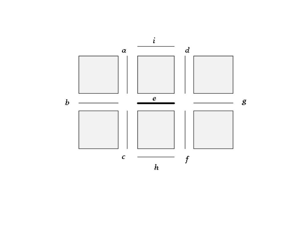
6

Crack edges surrounding central edge

The central edge e has a vertex at each of its ends and three possible
border continuations can be found from both of these vertices. 

Computer Vision

Segmentation

7

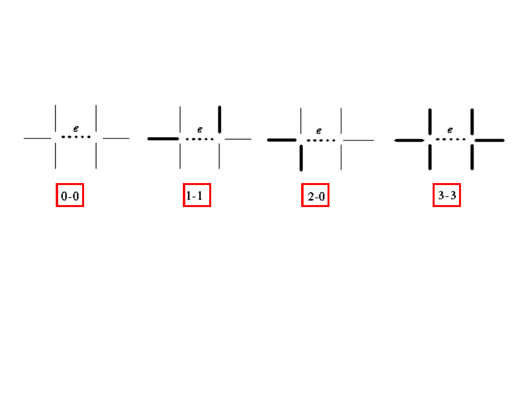
Edge Types and its influence

• 0-0 isolated

 negative influence

• 0-1 uncertain



weak positive

• 0-2, 0-3 dead end



negative influence

• 1-1 continuation 

strong positive

• 1-2, 1-3 continuation 

strong positive

•

2-2, 2-3, 3-3 bridge between borders  no influence on edge confidence

Computer Vision

Segmentation

8

Algorithm:

Edge Relaxation

1.

Evaluate Vertex Type:

is the number of edges emanating from

the vertex above a threshold value. (possible values are 0, 1, 2,

3.

2.

Evaluate Edge Type

: is determined by number of emerging

edges at each end. (0-0, 0-1, 0-2, 0-3, 1-1, 1-2, 1-3, 2-2, 2-3, 3-3)

3.

Update the confidence of each edge e according to its type

4.

Stop if all edge confidence have converged either to 0 or 1.

Note: Edge relaxation is an iterative method, with edge confidences converging
either to zero (edge termination) or one (the edge forms a border). 

Computer Vision

Segmentation

9

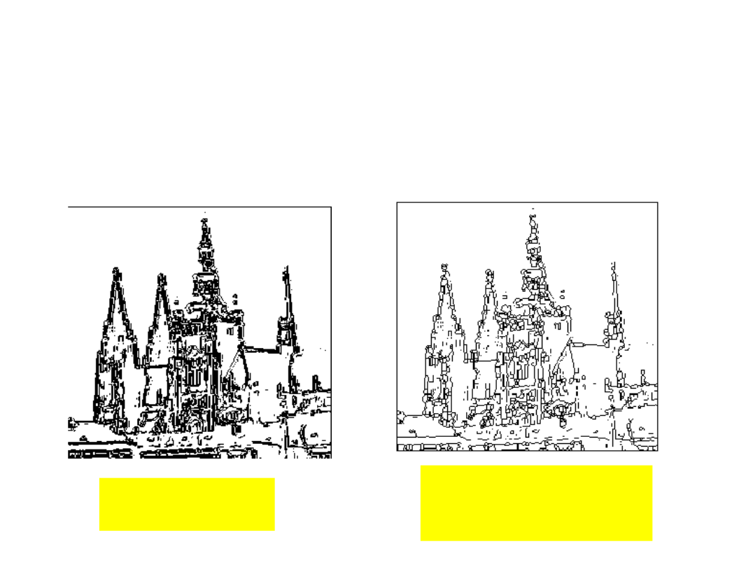
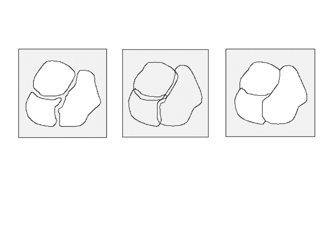
Effect of Edge Relaxation

After 10
iterations

After thinning using

non-maximal

suppression

Computer Vision

Segmentation

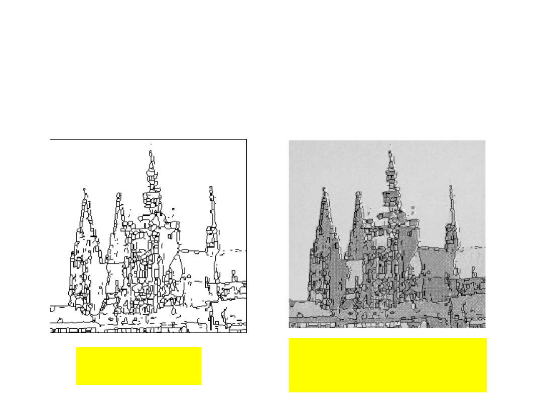
10

After 100
iterations

Borders after 100

iterations overlaid on

original

Effect of Edge Relaxation

Computer Vision

Segmentation

11



If region border is not known but regions have
been defined, borders can be detected.



During border tracing

three types of borders

can

be defined:

•

An

inner

region border is a subset of the region. 

•

An

outer

border is not a subset of the region. 

•

An

extended

border

Border Tracing

Computer Vision

Segmentation

12

Border Types

Inner

Boundary

Outer

Boundary

Extended

Boundary

The inner border is always part of a region but the outer border never
is. Therefore, if two regions are adjacent, they never have a common
border, which causes difficulties in higher processing levels with region
description, region merging, etc. 

The extended border defines single common border between adjacent
regions

 

Computer Vision

Segmentation

13

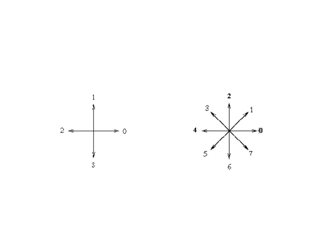
Connectivity Types

4 -

4 -

connectivity

connectivity

8 -

8 -

connectivity

connectivity

Computer Vision

Segmentation

14

1.

Search

image from top left till a starting pixel P

o

of new

region border is found.

2.

Define

dir

which stores the direction of the move from the

previous to the current border element.

3.

Search the 3x3 neighborhood of current pixel in anti-

clockwise direction beginning at

(dir+3) mod 4

The first pixel found is a new boundary element Pn. Update

dir value.

Algorithm:

Inner Border

Tracing

(4-connectivity)

dir = 3

1

0

2

Computer Vision

Segmentation

15

4.

If the current boundary element P

n

is equal to

the second border element P

1

and if the

previous border element P

n-1

is equal to P

0

stop.

Otherwise go to step 3.

5.

The detected inner border is represented by

P

0

... P

n-2

.

NOTE:

Algorithm does not determine edges of

region holes!

Algorithm:

Inner Border Tracing (cont.)

Computer Vision

Segmentation

16

1.

Trace inner boundary region boundary in 4-
connectivity until done.

2.

The outer boundary consists of non-region pixels
tested during the search process. Any

pixels

tested more than once

they are listed more than

once!

Algorithm:

Outer Border

Tracing

Computer Vision

Segmentation

17

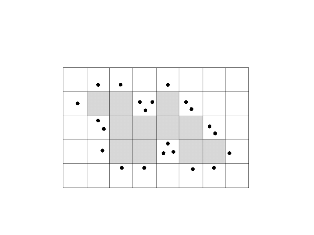
Demo:

Inner and Outer Border Tracing

Inner
Borde
r Pixel

Outer
Borde
r Pixel

detec.

once

Outer
Borde
r Pixel

detec.

twice

Computer Vision

Segmentation

18

Multiple Outer Border Example

Computer Vision

Segmentation

19

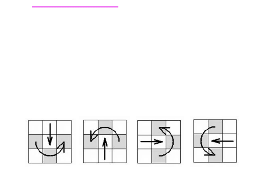
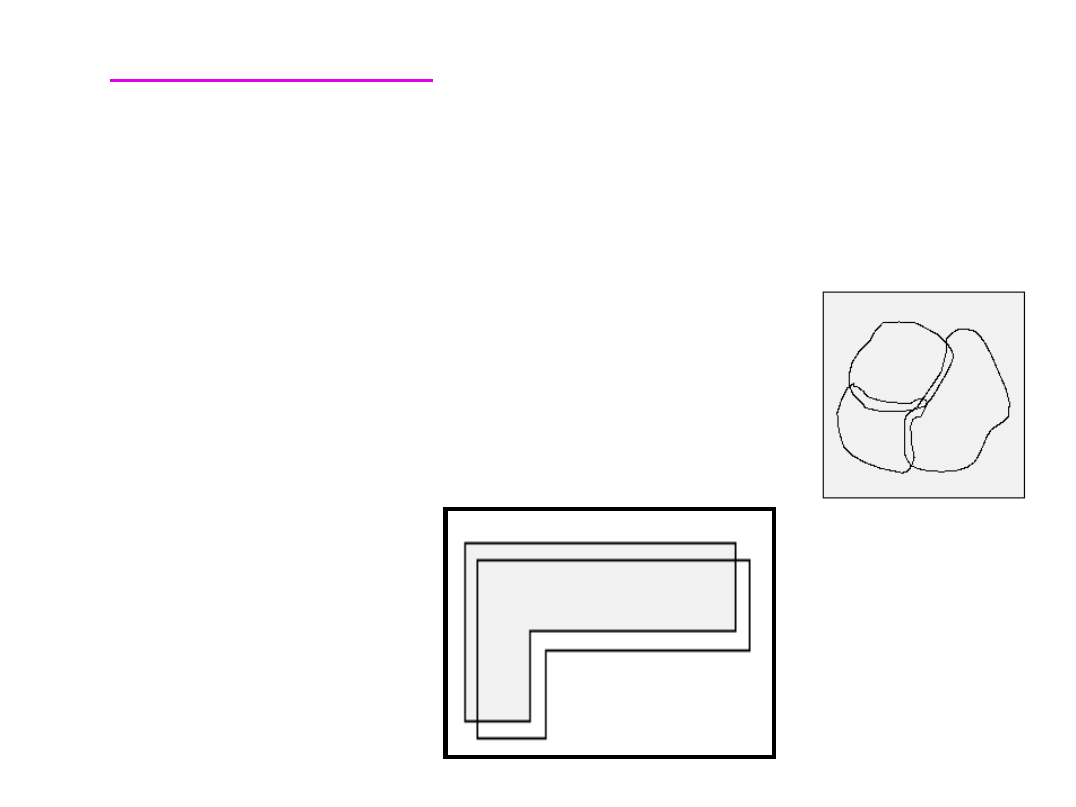
It is constructed

from the outer boundary

by:

1.

shifting all upper outer boundary points one pixel

down and right

2.

all left
 one pixel right

3.

all right
 one pixel down

4.

all lower
remain unchanged.

Algorithm:

Extended Border

Tracing

outer boundary

Computer Vision

Segmentation

20

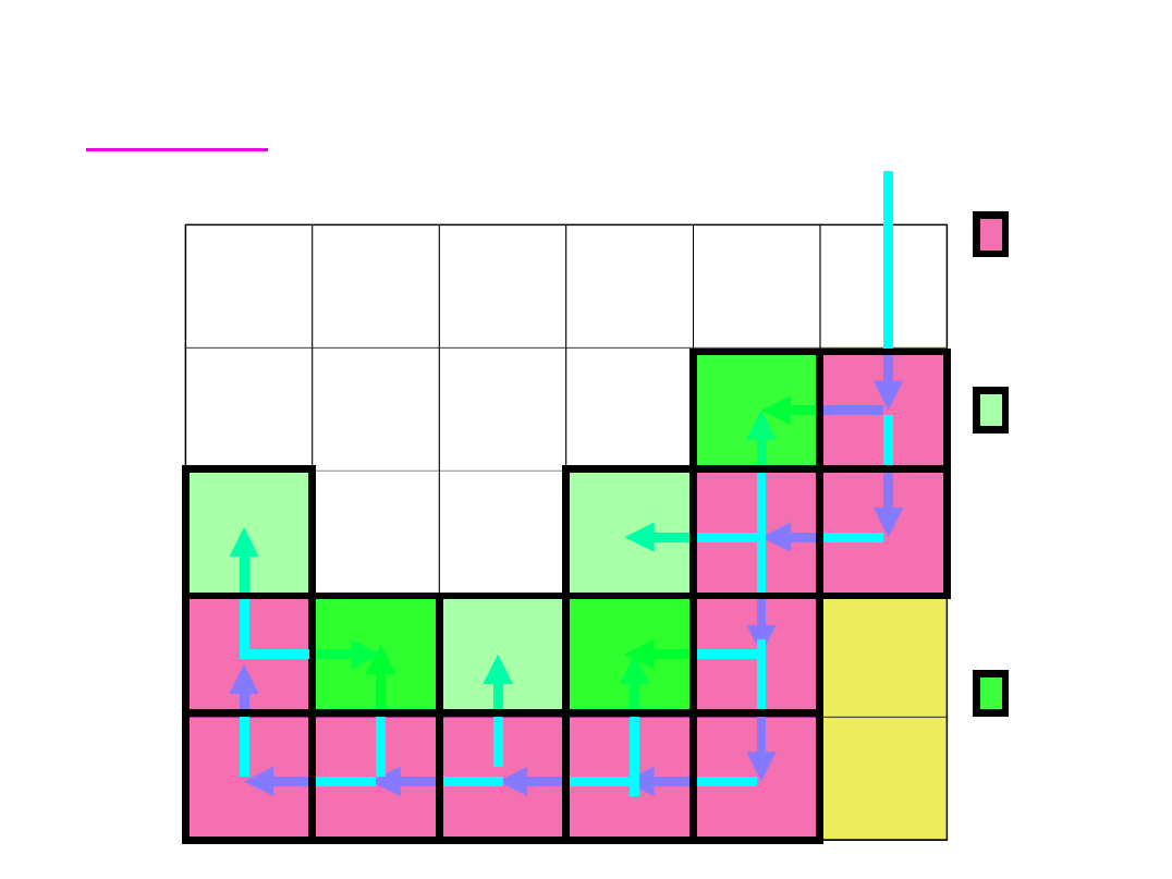
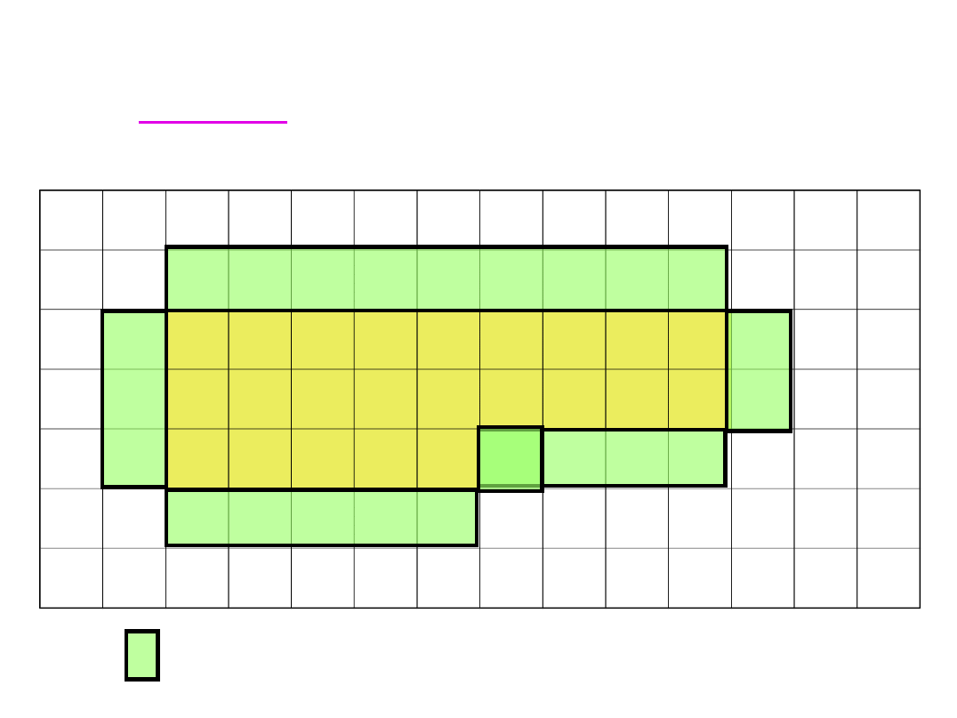
Demo:

Extended Border Tracing

Outer
Boundary

Computer Vision

Segmentation

21



Used when

a-priori information

about a

known

starting point and a known ending point

is

available.



The search is then for the

optimal path

that

connects those two points in a weighted graph.



Cost of a node

reflects the likelihood that the

border passes through that node.

Border Detection as Graph

Searching

Computer Vision

Segmentation

22

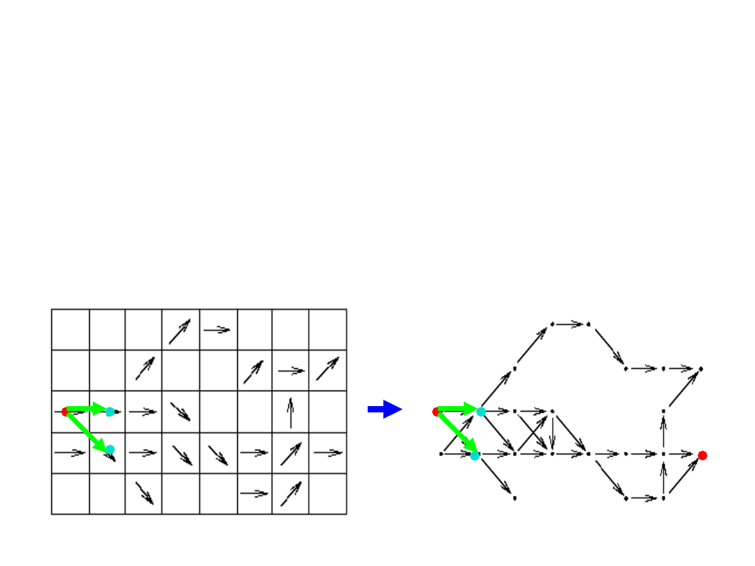
Heuristic Graph Search



The border detection process is transformed into
a search for the optimal path in the weighted
graph.

n

A

n

B

Computer Vision

Segmentation

23

1. Edge strength: Forming a border where the maximum

edge strength is obtained from all pixels in the image

2. Border curvature: minimize the difference in edge

directions in two consecutive border elements.

3. Proximity to an approximate border location

dist(x

i

, approximate_boundary)

4. Estimates of the distance to the goal (end-point) 

h(x

i

)= dist(x

i

, x

B

)

Cost Functions in

Graph

Searching

Computer Vision

Segmentation

24

1.

Expand the starting node n

A

and put all its successors

into an OPEN list with pointers back to n

A

. Evaluate the

cost function of each expanded node.

2.

If OPEN is empty, fail.

3.

Determine the node

n

i

from OPEN

with lowest cost and

remove it.

4.

If n

i

= n

B

, trace back for the optimum path.

Algorithm:

Heuristic Graph

Search

Computer Vision

Segmentation

25



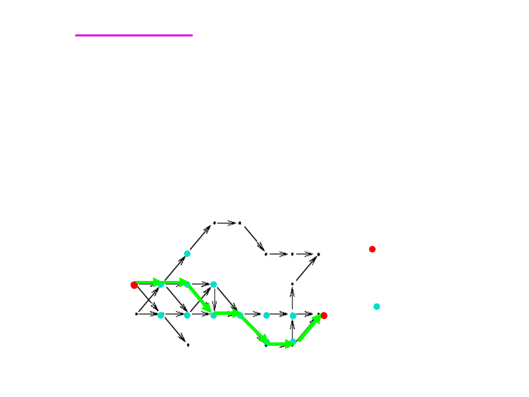
The border detection process is trans-formed into
a search for the optimal path in the weighted
graph.

Pixel in
OPEN list

Pixel on
optimum
path

n

A

n

B

Demo:

Heuristic Graph

Search

n

A

n

B

n

A

n

B

n

A

n

B

n

A

n

B

Computer Vision

Segmentation

26

The existence of a

path between start and end points is

not guaranteed

. Hence, if no node exists in OPEN list it

may be possible to expand node with non-significant edge

valued successors.

Problem: Extremely large number of expanded nodes in

OPEN list.

Some ‘bad’ nodes may be included which have

a low probability of generating the optimum

Graph Searching Issues

Computer Vision

Segmentation

27



Solution:

Some of the methods that make the solution

more practical (although which do not necessarily
generate the optimum path!) are:

1.

Pruning

the solution tree by:

• Deleting paths with high average cost per

unit length

• Deleting paths that are too short when the

number of nodes in OPEN exceeds a certain
limit

Graph Searching Issues Resolution

Computer Vision

Segmentation

28

2.

Least maximum cost:

Setting the cost of a path as the

most expensive arc in the path, hence path does not
necessarily grow with each step.

3.

Branch and bound:

The cost of a path is not allowed to

exceed a certain limit.

4.

Multi-resolution processing:

A sequence of two graph

search processes is performed. The first in a low resolution
and the second in a higher resolution.

Graph Searching Issues

Resolution(cont.)

Computer Vision

Segmentation

29



Efficient way of simultaneously searching for
optimal path from

multiple starting and ending

points.



Main idea

of optimality is:

“If the optimal path startpoint-endpoint goes through
a point E, then there exists an optimum path in both
its parts startpoint-E and E-endpoint.”

Border detection as

dynamic programming

Computer Vision

Segmentation

30

Demo:

Boundary Tracing as

dynamic programming

A

C

B

F

E

D

G

H

I

Start
Nodes

End
Nodes

7

2

6

1

3

8

2

5

3

4

5

2

7

6

D(2)

E(2)

F(1)

G(7)

H(3)

I(7)

Computer Vision

Segmentation

31



Same

modifications and principle for estimating the

objective function

are applied as before.



Using

the A-algorithm it is not necessary to

construct the entire graph

; in dynamic

programming a complete graph must be
constructed.



Hence,

heuristic search

may be more

efficient

with

respect to

computational

time. However,

dynamic

programming

is more

efficient

when simultaneously

searching

for

optimal path from

multiple starting

and ending points.

Dynamic Programming

versus Graph

Search

Computer Vision

Segmentation

32



Goal:
to link points by determining whether they lie on a curve

of specific shape.



Computational Complexity:
With n points

to find the line connecting

each two:

Complexity = n x (n-1)

= n

2

Hough transform is computationally attractive!

HoughTransform

Computer Vision

Segmentation

33

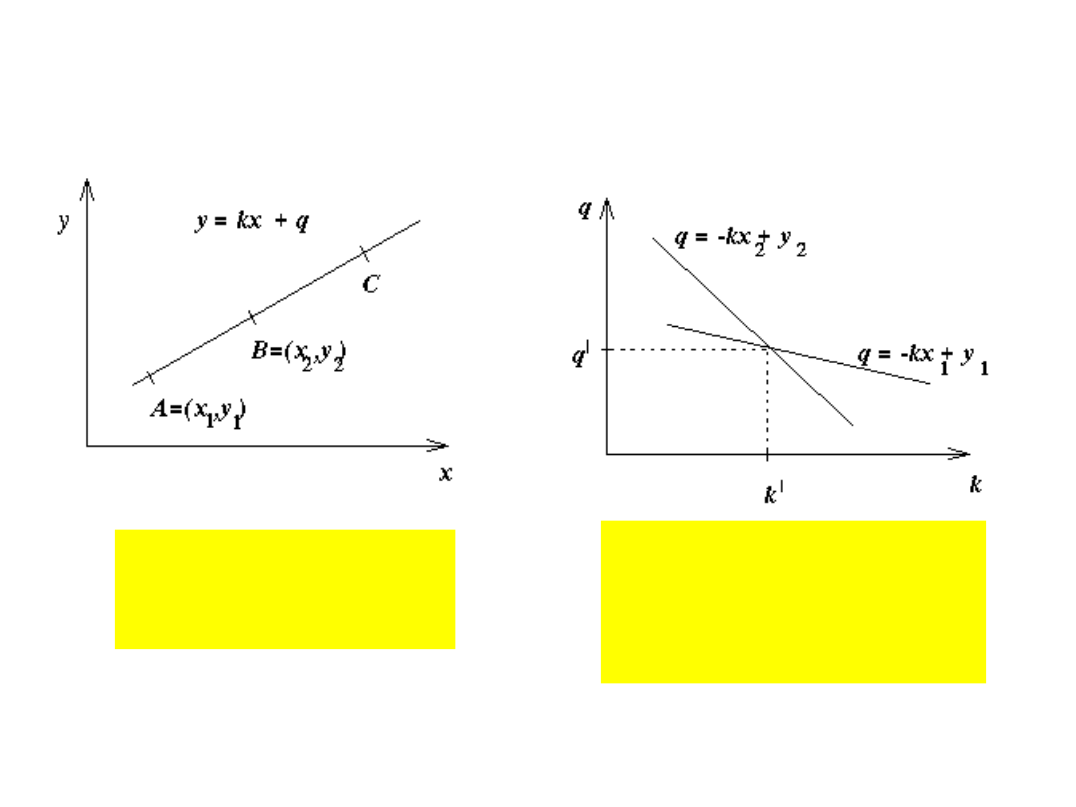
Straight Line

All points on line

y = kx + q

All lines through
point

q = y - kx

Computer Vision

Segmentation

34

1. Parameter space is divided into accumulator
cells A, all, initially, set to zero.
2. For every point p(x,y) in image change k in
the range and calculate q
3. For each x

p

, y

p

pair of a point p

A(k

p

, q

p

) = A(k

p

, q

p

) + 1

Algorithm:

Hough Transform for line

detection

Computer Vision

Segmentation

35

4. At the end the value of A(k

i

, q

j

) corresponds to the number

of points that lie on the line:

y = - k

i

x + q

j



Accuracy

of co-linearity is determined by the size of

subdivisions.



Having k subdivisions,

computational complexity

is now

n x k

where k is the number of subdivisions
i.e

. linear

in n!

Algorithm:

Hough Transform for line

detection (cont.)

Computer Vision

Segmentation

36

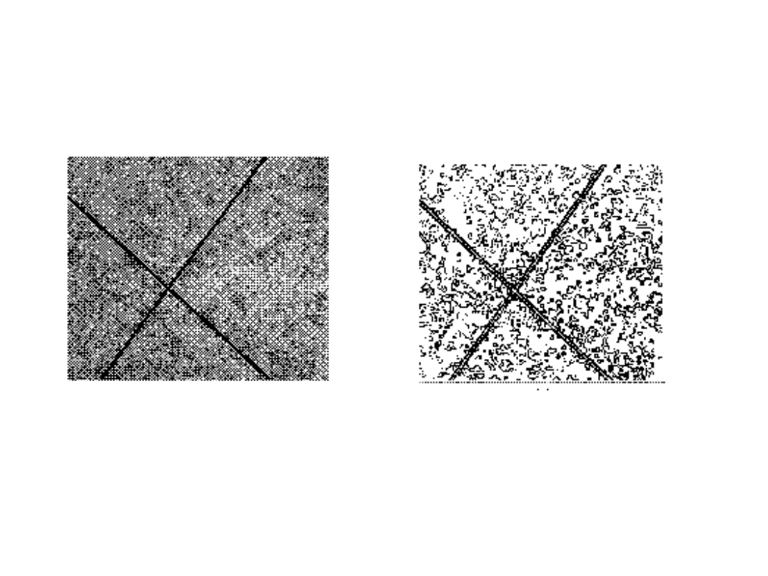
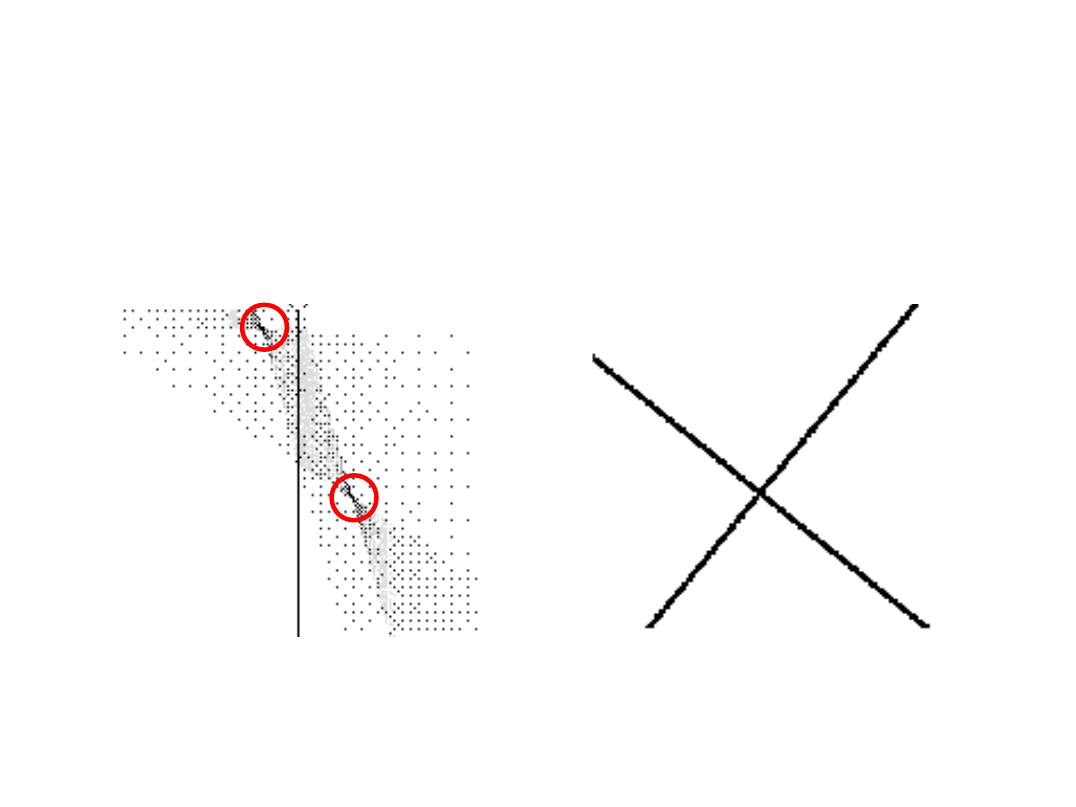
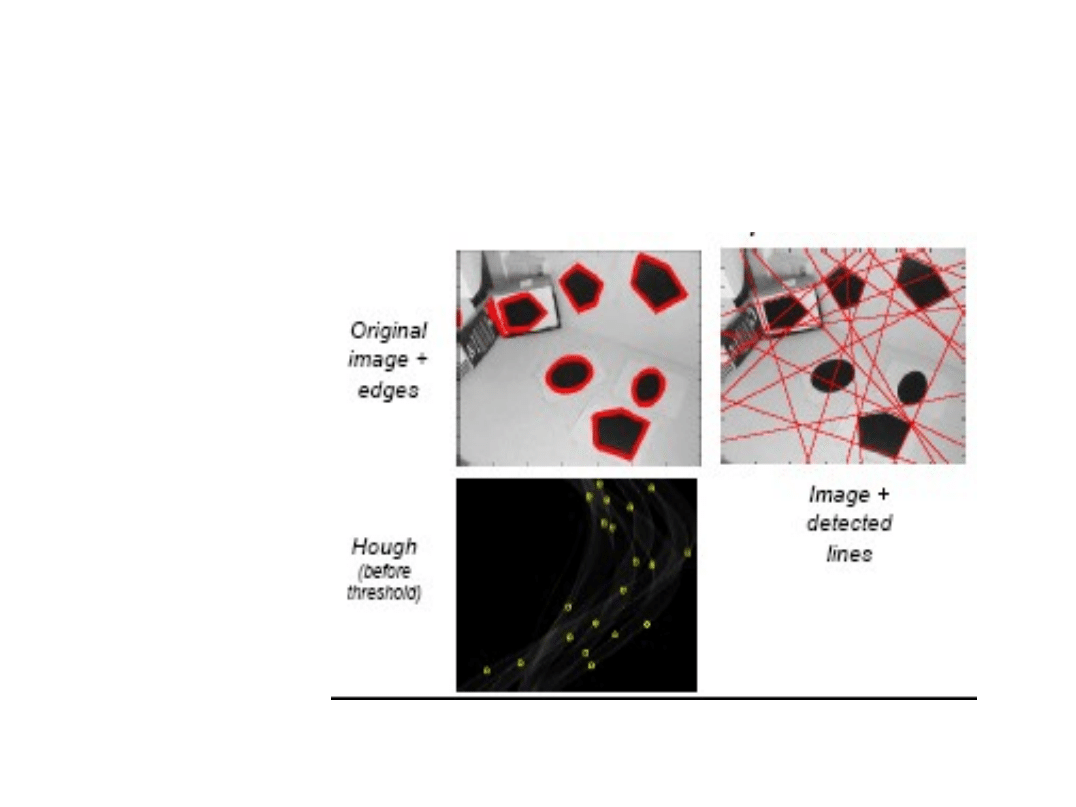
Hough Transform Line Detection

Example

Original Image

Notice: many non-

belonging edges

Edge Image

Computer Vision

Segmentation

37

Parameter
Space

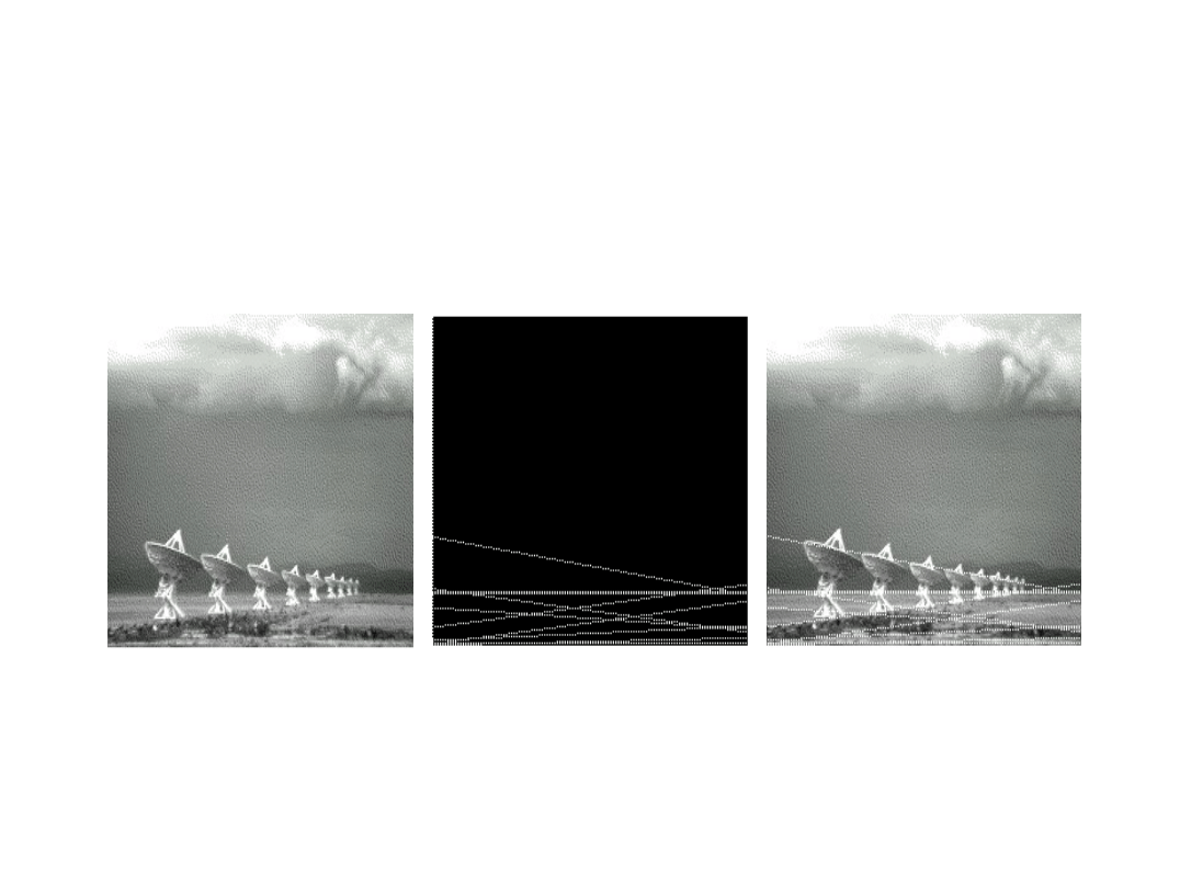
Detected Lines

Hough Transform Line Detection

Example

Computer Vision

Segmentation

38

Hough Transform Line Detection

Example

Original
Image

Original Image
with
superimposed
Lines

Detected
Lines

Example:

Computer Vision

Segmentation

39

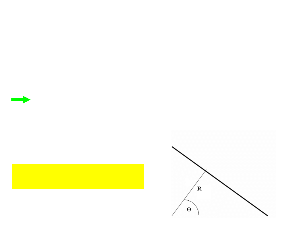
Line representation



Problem

: if line is vertical then

q =

∞

Solution:

use Normal representation:

R

y

x









sin

cos

Computer Vision

Segmentation

40

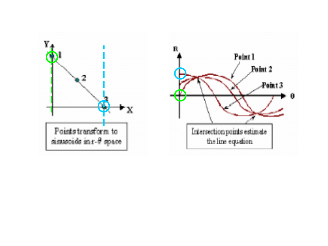
(cont) Line representation

The Normal representation approach is similar

BUT

:

•Loci are sinusoidal! i.e. each point in the x-y plane yields
one sinusoidal curve on the p-θ plane and

•m co-linear points in x-y plane yield m sinusoidal curves in
the p- plane intersecting at a certain p and θ corresponding
to the line connecting them.

•Range of θ is 0 to π

Computer Vision

Segmentation

41

HoughTransform Example

Note:

Axis of R-θ parameter space is rotated 90

o

!

Computer Vision

Segmentation

42



If looking for

circles

, instead of lines the analytic

expression is:



As there are

3 parameters

then the accumulator

data structure must be three dimensional, i.e.
the accumulator cell is A(a,b,r).

Hough Transform for Circle Detection

2

2

)

(

2

)

(

r

b

y

a

x









Computer Vision

Segmentation

43



Again the Hough transform is applied to each point
whose edge magnitude exceeds a certain threshold.



The processing results correspond to points of local
maxima of accumulator cells in the parameter space
a,b of the center point of the circle and the radius r.



If

the length of the

radius

of the circle searched

is

known

then we can deal with a 2-dimensional

parameter space (for center point coordinates a,b).



One

heuristic

may be used: to

weight the

contribution of

a point

to an accumulator cell by its

edge magnitude.



Algorithm:

Hough Transform

for Circle

Detection

Computer Vision

Segmentation

44

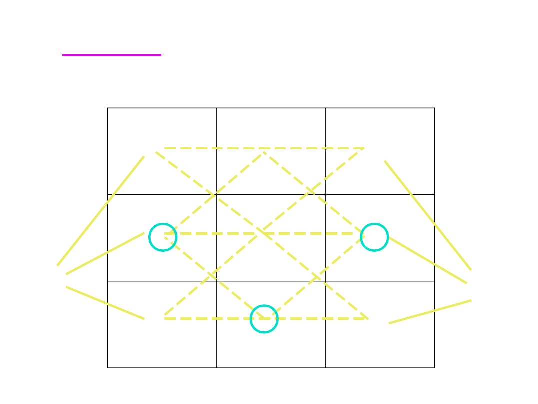
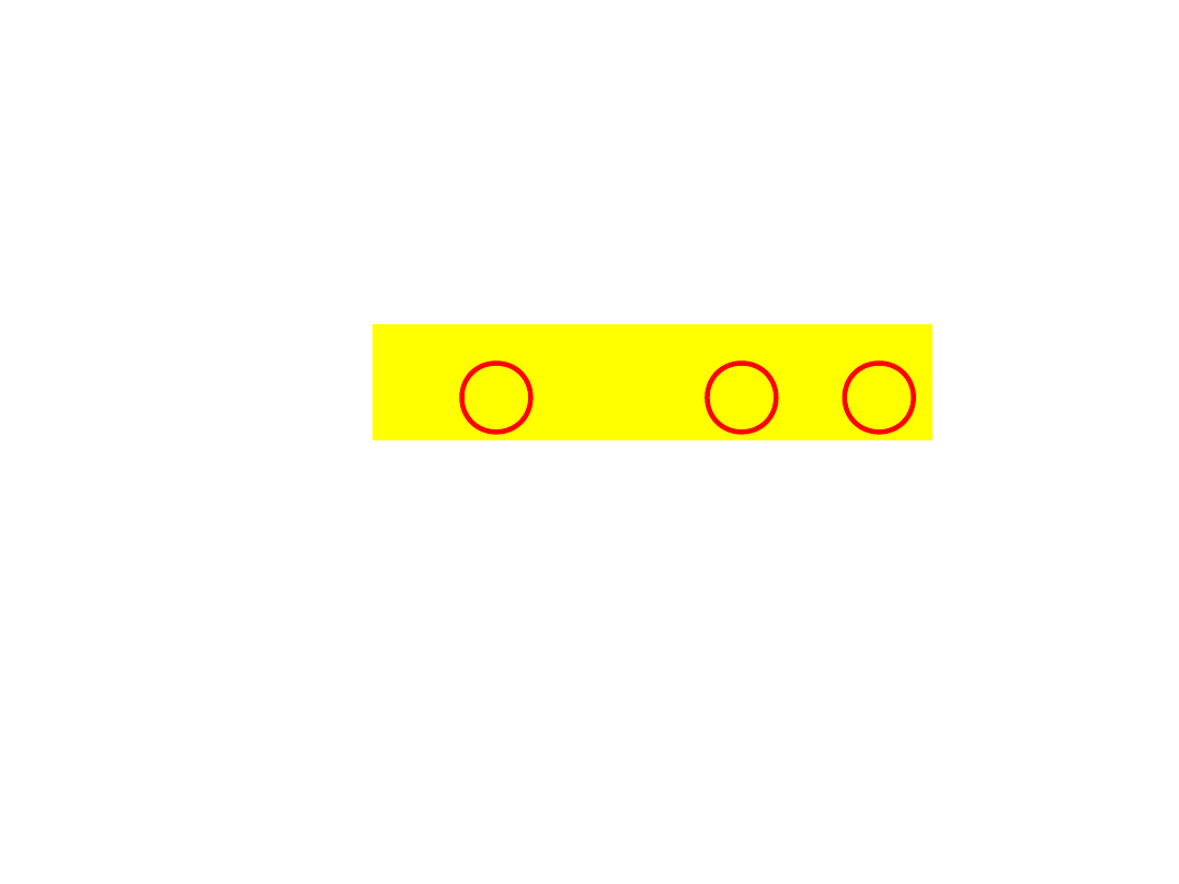
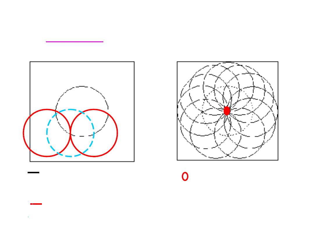
Demo:

Hough Transform

Original Circle

●

●

●

●

point on circle

circles passing through

point

loci of centers of circles passing through
point

Intersection of circles

specifies center of

original circle

●

point on circle

circles passing through

point

Computer Vision

Segmentation

45

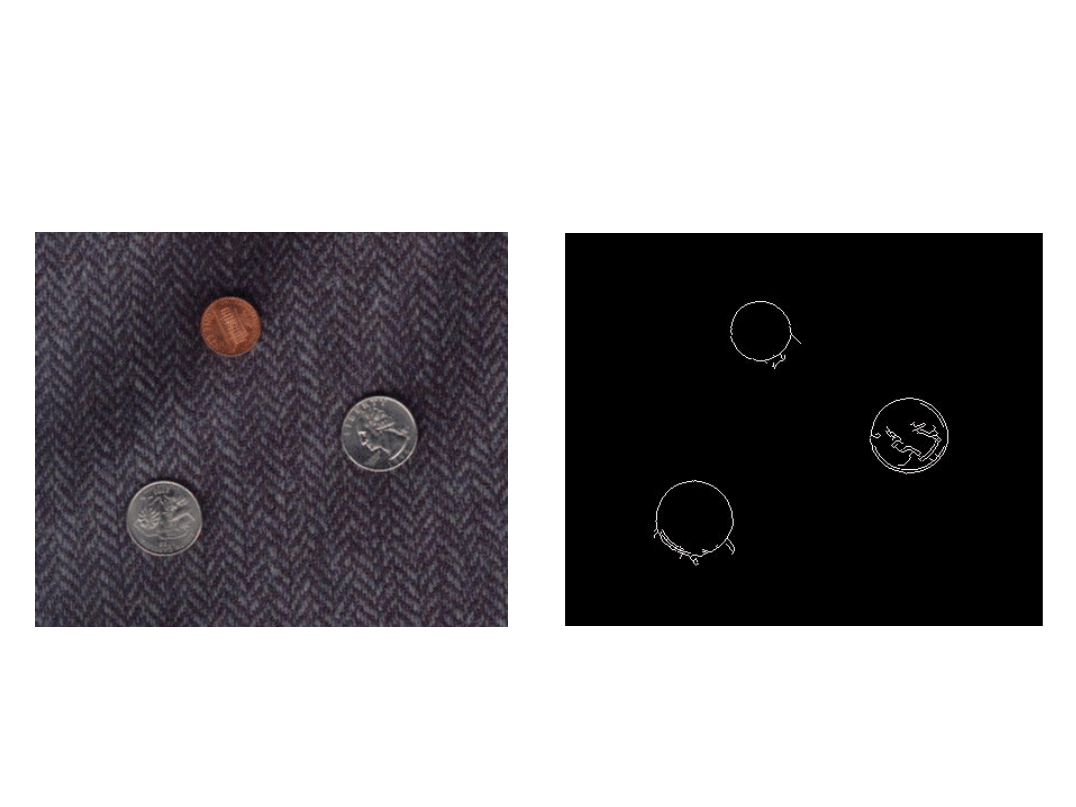
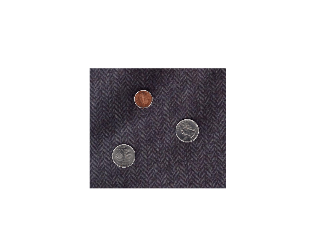
Hough Transform Example

Original Image

Edge Image

Computer Vision

Segmentation

46

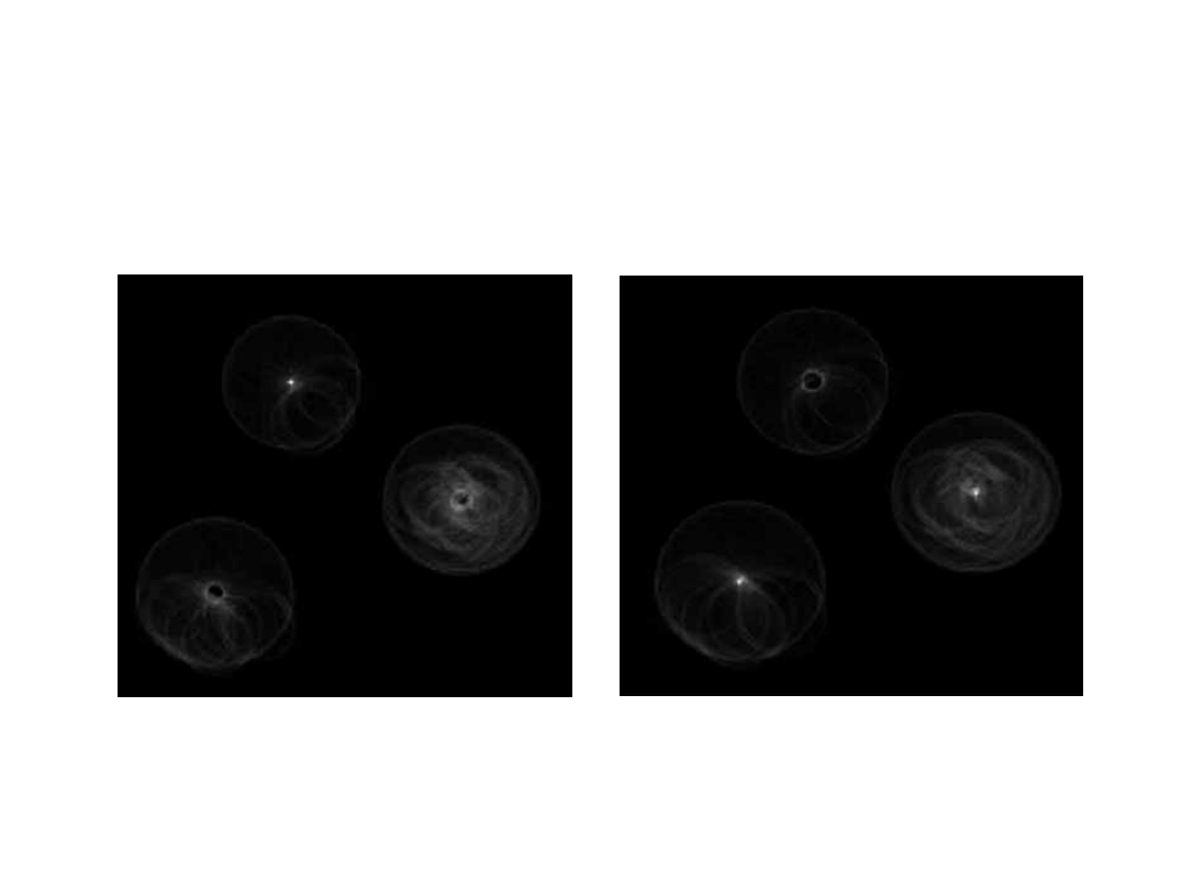
HoughTransfor

m for Penny

HoughTransfor

m for Quarters

Hough Transform Example

Computer Vision

Segmentation

47

Detected Coins

Hough Transform Example