
Technical Report Documentation Page
1. Report No.
FHWA/TX-09/0-5530-1
2. Government Accession No.
3. Recipient's Catalog No.
4. Title and Subtitle
PREDICTION OF EMBANKMENT SETTLEMENT OVER SOFT
SOILS
5. Report Date
December 2008
Published: June 2009
6. Performing Organization Code
7. Author(s)
Vipulanandan, C., Bilgin, Ö., Y Jeannot Ahossin Guezo, Vembu, K.
and Erten, M. B.
8. Performing Organization Report No.
Report 0-5530-1
9. Performing Organization Name and Address
University of Houston
Department of Civil and Environmental Engineering
Houston, Texas 77204-4003
10. Work Unit No. (TRAIS)
11. Contract or Grant No.
Project 0-5530
12. Sponsoring Agency Name and Address
Texas Department of Transportation
Research and Technology Implementation Office
P. O. Box 5080
Austin, Texas 78763-5080
13. Type of Report and Period Covered
Technical Report:
September 2005 - October 2008
14. Sponsoring Agency Code
15. Supplementary Notes
Research performed in cooperation with the Texas Department of Transportation and the Federal Highway
Administration.
Research Project Title: Prediction of Embankment Settlement Over Soft Soils
URL: http://tti
.tamu.edu/documents/0-5530-1.pdf
16. Abstract
The objective of this project was to review and verify the current design procedures used by TxDOT
to estimate the total and rate of consolidation settlement in embankments constructed on soft soils. Methods
to improve the settlement predictions were identified and verified by monitoring the settlements in two
highway embankments over a period of 20 months. Over 40 consolidation tests were performed to quantify
the parameters that influenced the consolidation properties of the soft clay soils. Since there is a hysteresis
loop during the unloading and reloading of the soft CH clays during the consolidation test, three
recompression indices (C
r1
, C
r2
, C
r3
) have been identified with a recommendation to use the recompression
index C
r1
(based on stress level) to determine the settlement up to the preconsolidation pressure. Based on the
laboratory tests and analyses of the results, the consolidation parameters for soft soils were all stress
dependent. Hence, when selecting representative parameters for determining the total and rate of settlement,
expected stress increases in the ground should be considered. Also the 1-D consolidation theory predicted
continuous consolidation settlement in both of the embankments investigated. The predicted consolidation
settlements were comparable to the consolidation settlement measured in the field. Constant Rate of Strain
test can be used to determine the consolidation parameters of the soft clay soils. The effect of Active Zone
must be considered in designing the edges of the embankments and the retaining walls.
17. Key Words
Active Zone, Consolidation, Embankment, Field
Tests, Recompression Indices, Settlement, Soft Soils
18. Distribution Statement
No restrictions. This document is available to the
public through NTIS:
National Technical Information Service
5285 Port Royal Road
Springfield, Virginia 22161
19. Security Classif.(of this report)
Unclassified
20. Security Classif.(of this page)
Unclassified
21. No. of Pages
210
22. Price
Form DOT F 1700.7
(8-72) Reproduction of completed page authorized


Prediction of Embankment Settlement Over Soft Soils
Project Report No. TxDOT 0-5530-1
Final Report
by
C. Vipulanandan Ph.D., P.E.
Ö. Bilgin, Ph.D., P.E.
Y. Jeannot Ahossin Guezo
Kalaiarasi Vembu
and
Mustafa Bahadir Erten
I G M A T
C
1994
Performed in cooperation with the
Texas Department of Transportation
and the
Federal Highway Administration
June 2009
Center for Innovative Grouting Materials and Technology (CIGMAT)
Department of Civil and Environmental Engineering
University of Houston
Houston, Texas 77204-4003
Report No. CIGMAT/UH 2009-6-1


v
ENGINEERING DISCLAIMER
The contents of this report reflect the views of the authors, who are responsible
for the facts and the accuracy of the data presented herein. The contents do not
necessarily reflect the official views or policies of the Texas Department of
Transportation or the Federal Highway Administration. This report does not constitute a
standard or a regulation.
There was no art, method, process, or design that may be patentable under the
patent laws of the United States of America or any foreign country.

vi
ACKNOWLEDGMENTS
This project was conducted in cooperation with Texas Department of
Transportation (TxDOT) and Federal Highway Administration (FHWA).
The researchers thank the TxDOT for sponsoring this project. Also thanks are
extended to the Project Coordinator K. Ozuna (Houston District), Project Director S. Yin
(Houston District) and Project Committee Members R. Willammee (Fort worth District),
M. Khan (Houston District), D. Dewane (Austin District) R. Bravo (Pharr District) and P.
Chang (FHWA).

vii
PREFACE
Settlement of highway embankments over soft soils is a major problem
encountered in maintaining highway facilities. The challenges to accurately predict the
total and rate of consolidation settlements are partly due to the uncertainties in field
conditions, laboratory testing, interpretations of laboratory test data, and assumptions
made in the development of the 1-D consolidation theory. Hence, there is a need to
investigate methods to better predict the settlement of embankments on soft soils.
The objective of this project was to review and verify the current design
procedures used in TxDOT projects to estimate the total and rate of consolidation
settlements in embankments constructed on soft soils. Methods to improve the settlement
predictions were identified and verified by monitoring the settlements in two highway
embankments over a period of 20 months. Over 40 consolidation tests were performed to
quantify the parameters that influence the consolidation properties of the soft clay soils.
Based on the laboratory tests and analyses of the results, the consolidation parameters for
soft soils were all stress dependent. Hence, when selecting representative parameters for
determining the total and rate of settlement, expected stress increases in the ground
should be considered. Also the 1-D consolidation theory predicted continuous
consolidation settlement in both of the embankments investigated. The predicted
consolidation settlements were comparable to the consolidation settlement measured in
the field.
This report reviewed the current TxDOT project approach to predict the total and
rate of consolidation settlements of embankments over soft soils. Based on the laboratory
and field investigations, methods to further improve the embankment settlement
predictions have been recommended.

viii
ABSTRACT
The prediction of embankment settlement over soft soils (defined by the
undrained shear strength and/or Texas Cone Penetrometer value) has been investigated
for many decades. The challenges mainly come from the uncertainties about the geology,
subsurface conditions, extent of the soil mass affected by the new construction, soil
disturbances during sampling and laboratory testing, interpretations of laboratory test
data, and assumptions made in the development of the one-dimensional consolidation
theory. Since the soft soil shear strength is low, the structures on the soft soils are
generally designed so that the increase in the stress is relatively small and the total stress
in the ground will be close to the preconsolidation pressure. Hence there is a need to
investigate methods to better predict the settlement of embankments on soft soils.
The objective of this project was to review and verify the current design
procedures used by TxDOT to estimate the total and rate of consolidation settlement in
embankments constructed on soft soils. Methods to improve the settlement predictions
were identified and verified by monitoring the settlements in two highway embankments
over a period of 20 months. Over 40 consolidation tests were performed to quantify the
parameters that influenced the consolidation properties of the soft clay soils. Since there
is a large hysteresis loop during the unloading and reloading of the soft CH clays during
the consolidation test, three recompression indices (C
r1
, C
r2
, C
r3
) have been identified
with the recommendation to use the recompression index C
r1
(based on stress level) to
determine the settlement up to the preconsolidation pressure. Based on the laboratory
tests and analyses of the results, the consolidation parameters for soft soils were all stress
depended. Hence, when selecting representative parameters for determining the total and
rate of settlement, expected stress increases in the ground should be considered. Linear
and nonlinear relationships between compression indices of soft soils and moisture
content and unit weight of soils have been developed. Also the 1-D consolidation theory
predicted continuing consolidation settlement in both of the embankments investigated.
The predicted consolidation settlements were comparable to the consolidation settlement
measured in the field. The Constant Strain Rate test can be used to determine the

ix
consolidation parameters of the soft clay soils. The effect of Active Zone must be
considered in designing the edges of the embankments and the retaining walls.


xi
SUMMARY
The prediction of consolidation settlement magnitudes and settlement rates in soft
soils (defined by the undrained shear strength and/or Texas Cone Penetrometer value) is a
challenge and has been investigated by numerous researchers since the inception of
consolidation theory by Terzaghi in the early 1920s. The challenges mainly come from
the uncertainties about the geology, subsurface conditions, extent of the soft soil mass
affected by the new construction, soil disturbances during sampling and preparation of
samples for laboratory testing, interpretations of laboratory test data, and assumptions
made in the development of the one-dimensional consolidation theory. Since the soft soil
shear strength is low, the structures on the soft soils are generally designed such that the
increase in the stress is relatively small and the total stress in the ground will be close to
the preconsolidation pressure. Hence, there is a need to further investigate methods to
better predict the settlement of embankments on soft soils.
The objective of this project was to review and verify the current design
procedures used by TxDOT to estimate the total and rate of consolidation settlements in
embankments constructed on soft soils. The review of the design procedures indicated
that the methods used to determine the increase in in-situ stresses and the
preconsolidation pressure, and the testing method used to determine the consolidation
properties were appropriate except for the approach used for determining the rate of
settlement. Also the practice of using the recompression index was not clearly defined.
In order to verify the prediction methods, two highway embankments on soft clay
with settlement problems were selected for detailed field investigation. Soil samples
were collected from nine boreholes for laboratory testing. The embankments were
instrumented and monitored for 20 months to measure the vertical settlement, lateral
movement, and changes in the pore water pressure. Over 40 consolidation tests were
performed to investigate the important parameters that influenced the consolidation
settlements of the soft soils.
Based on this study, it was determined that the increase in in-situ stresses due to
the embankment are relatively small (generally less than the preconsolidation pressure),

xii
and hence using the proper recompression index became more important to estimate the
settlement. Since there is a large hysteresis loop during the unloading and reloading of
the soft CH clays during the consolidation test, three recompression indices (C
r1
, C
r2
, C
r3
)
have been identified and with the recommendation to use the recompression index C
r1
(based on stress level) to determine the settlement up to the preconsolidation pressure.
Based on the laboratory tests and analyses of the results, the consolidation parameters
such as compression index (C
c
), recompression indices (C
r
), and coefficient of
consolidation (C
v
) for soft soils were all stress dependent. Hence, when selecting
representative parameters for determining the total and rate of settlements, expected
stress increases in the ground should be considered. Linear and nonlinear relationships
between compression indices of soft soils and moisture content and unit weight of soils
have been developed. Also the 1-D consolidation theory predicted continuous
consolidation settlement in both the embankments investigated. The predicted
consolidation settlements were comparable to the consolidation settlement measured in
the field. The pore water pressure measurements in some cases did not indicate
consolidation because they may have been located close to the bottom drainage. In one
case excess pore water pressures were measured, indicting consolidation was in progress.
The Active Zone influenced the movements at the edge of the embankments.
Movements in the Active Zone influenced the crack movements in the retaining wall
panels. The Constant Rate of Strain (CRS) test can be used to determine the consolidation
properties of soft clay soils. The strain rate used during the test influenced the coefficient
of consolidation.

xiii
RESEARCH STATEMENT
This research project was to review the current design procedures and verify the
applicability of conventional consolidation theory to predict the total and rate of
settlements of embankments over soft clays. The study included field sampling,
laboratory testing, and monitoring the settlement of two embankments for a period of up
to 20 months. Based on this study, further improvements have been suggested to better
predict the rate and total settlements of embankment over soft clay soils.
The report will be a guidance document for TxDOT engineers on instrumenting
embankments for measuring consolidation settlement and monitoring changes in the
Active Zone. Also the Constant Rate Strain (CRS) test has been recommended as an
alternative test to determine the consolidation properties of soft soils.


TABLE OF CONTENTS
Page
LIST OF FIGURES .......................................................................................................
..xv
ii
LIST OF TABLES .........................................................................................................xxii
i
1.
INTRODUCTION ...................................................................................................... 1
1.1.
General ................................................................................................................ 1
1.2.
Objectives ........................................................................................................... 3
1.3.
Organization ........................................................................................................ 3
2.
SOFT SOILS AND HIGHWAY EMBANKMENT ................................................... 5
2.1.
General ................................................................................................................ 5
2.2.
Soft Clay Soil Definition .................................................................................... 5
2.3.
Embankment Settlement ..................................................................................... 6
2.4.
Behavior of Marine and Deltaic Soft Clays ...................................................... 23
3.
DESIGN AND ANALYSIS OF HIGHWAY EMBANKMENTS ........................... 43
3.1.
Highway Embankments .................................................................................... 43
3.2.
Summary and Discussion ................................................................................ 100
4.
LABORATORY TESTS AND ANALYSIS .......................................................... 103
4.1.
Introduction ..................................................................................................... 103
4.2.
Tests Results ................................................................................................... 104
4.3.
Soil Characterization ....................................................................................... 119
4.4.
Preconsolidation Pressure (
σ
p
) ........................................................................ 120
4.5.
Compression Index (C
c
) .................................................................................. 124
4.6.
Recompression Index (C
r
) .............................................................................. 132
4.7.
Coefficient of Consolidation (C
v
) ................................................................... 137
4.8.
Constant Rate of Strain (CRS) Test (ASTM D 4186-86) ............................... 141
xv

4.9.
Summary ......................................................................................................... 145
5.
FIELD STUDY ....................................................................................................... 147
5.1.
Introduction ..................................................................................................... 147
5.2.
Site History and Previous Site Investigation .................................................. 148
5.3.
Instrumentation ............................................................................................... 150
5.4.
NASA Road 1 Embankment Instrumentation ................................................. 154
5.5.
SH3 Embankment Instrumentation and Results ............................................. 154
5.6.
NASA Road 1 (Project 4) ............................................................................... 171
5.7.
Summary and Discussion ................................................................................ 173
6.
CONCLUSIONS AND RECOMMENDATIONS ................................................. 177
7.
REFERENCES ....................................................................................................... 181
xvi

LIST OF FIGURES
Page
Fig. 2.1. Typical Configuration of Soil Layers under an Embankment. ............................. 7
Fig. 2.2. Field Condition Simulation in Laboratory Consolidation Test. ......................... 12
Fig. 2.3. Typical e – log
σ
v
Relationship for Overconsolidated Clay. ............................ 13
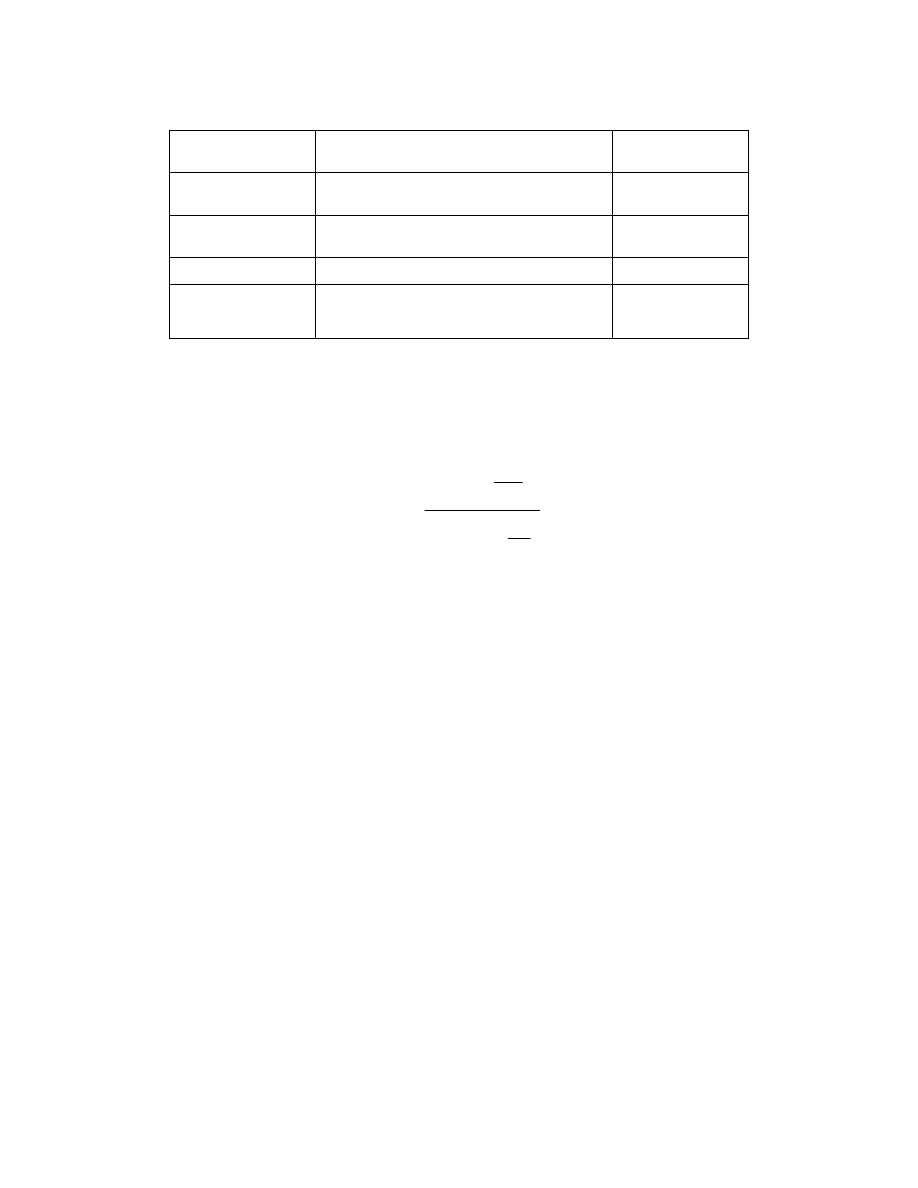
Fig. 2.4. Constant Rate of Strain (CRS) Consolidation Cell Used at the University
of Houston (GEOTAC Company 2006). .............................................................. 17
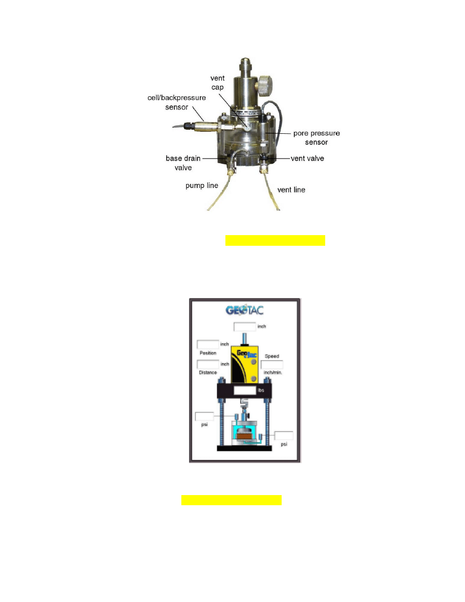
Fig. 2.5. Schematic of CRS Test Frame Used at the University of Houston
(GEOTAC Company 2006). ................................................................................. 17
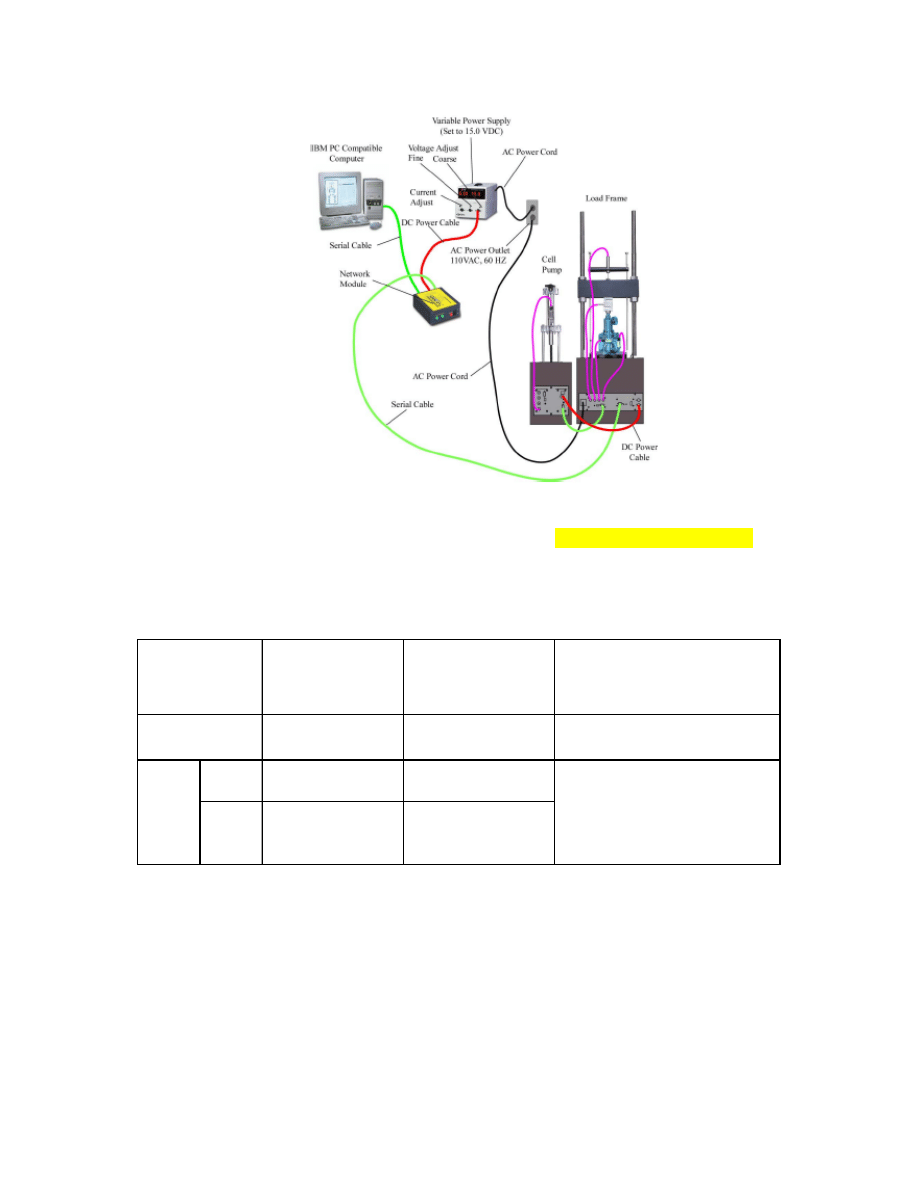
Fig. 2.6. Commercially Available CRS Test System (GEOTAC Company 2006). ......... 18
Fig. 2.7. 2:1 Method for Vertical Stress Distribution (Holtz and Kovacs 1981). ............. 20
Fig. 2.8. Vertical Stress Due to a Flexible Strip Load (Das 2006). .................................. 21
Fig. 2.9. Embankment Loading Using Osterberg’s Method (Das 2006). ......................... 22
Fig. 2.10. Locations of Soft Clay Soils Used for the Analysis. ........................................ 26
Fig. 2.11. Rate of Sedimentation of Different Types of Clay Deposits (Leroueil
1990). .................................................................................................................... 27
Fig. 2.12. Probability Distribution Function for the Undrained Shear Strength (a)
Marine Clay and (b) Deltaic Clay. ........................................................................ 34
Fig. 2.13. Liquid Limit versus Natural Water Content for the Soft Clays (a)
Marine Clay and (b) Deltaic Clay. ........................................................................ 35
Fig. 2.14. Plasticity Index chart of Deltaic (42 Data Sets) and Marine Soft Clay
Soils....................................................................................................................... 36
Fig. 2.15. Predicted and Measured Relationships for Marine and Deltaic Clays. ............ 37
Fig. 2.16. Relationship between Undrained Shear Strength (S
u
) and
Preconsolidation Pressure (
σ
p
). ............................................................................. 39
Fig. 3.1. Houston Area with the Selected Four Embankments. ........................................ 44
Fig. 3.2. Variation of TCP Blow Counts with Depth (Borehole 99-1a.). ......................... 47
Fig. 3.3. (a) Variation of Moisture Content (MC) with Depth (z) and (b) Change
of Moisture Content with Change in Depth (
ΔMC/Δz). ....................................... 48
Fig. 3.4. Variation of Undrained Shear Strength with Depth (Borehole 99-1a). .............. 49
Fig. 3.5. e – log
σ’ of the Two Consolidation Tests Performed on TxDOT Project
for 1A Embankment Design and Their Respective Compression and
Recompression Index versus log
σ’ Curves (Project 1: I-10 @ SH-99). ............. 51
Fig. 3.6. Profile of the Soil Layers for Settlement Calculation (Project 1)....................... 52
xvii

Fig. 3.7. Comparison of Stress Increase Obtained Using the Osterberg, 2:1, and
TxDOT Methods (Project 1). ................................................................................ 53
Fig. 3.8. Comparison of the Rate of Settlement by Various Methods of
Estimation. ............................................................................................................ 58
Fig. 3.9. Variation of TCP Blow Counts with Depth (Project 2). .................................... 60
Fig. 3.10. (a) Variation of Moisture Content (MC) with Depth (z) and (b) Change
of Moisture Content with Change in Depth (
ΔMC/Δz) (Project 2). ..................... 64
Fig. 3.11. Variation of Undrained Shear Strength with Depth (from the Four
Borings) (Project 2). .............................................................................................. 65
Fig. 3.12. Profile of the Soil Layers for Settlement Calculation (Project 2). .................... 66
Fig. 3.13. Comparison of Stress Increase Obtained Using Osterberg and 2:1 and
TxDOT Methods. .................................................................................................. 68
Fig. 3.14. Effect of Layering on the Rate of Settlement (Project 2). ................................ 73
Fig. 3.15. Profile of the Retaining Wall No. 2E, Not to Scale (Project 3 Drawing
22). ........................................................................................................................ 75
Fig. 3.16. Location of the Borings Used in the Field (Drawings 13 and 14). ................... 75
Fig. 3.17. Variation of TCP Blow Counts with Depth (Project 3).................................... 76
Fig. 3.18. (a) Variation of Moisture Content (MC) with Depth (z) and (b) Change
of Moisture Gradient with Depth (
ΔMC/Δz) (Project 3). ..................................... 79
Fig. 3.19. Variation of Undrained Shear Strength with Depth (Project 3). ...................... 80
Fig. 3.20. (a) e – log
σ’ Relationship for the Three Samples and (b) Variation of
Compression Index with log
σ’ (Project 3). ......................................................... 82
Fig. 3.21. Profile of the Soil Layers for Settlement Calculation (Project 3). .................... 83
Fig. 3.22. Variation of Stress Increase with Depth at the Center and at the Toe of
the Embankment Using the Osterberg Method (Project 3). .................................. 84
Fig. 3.23. Comparison of TxDOT Rate of Settlement Estimation at the Center of
the Embankment with New Estimation Using the Same Data. ............................ 87
Fig. 3.24. Comparative Graph Showing the Effect of Layering on the Rate of
Settlement at the Center of the Embankment (Project 3). .................................... 89
Fig. 3.25. Rate of Settlement at the Toe of the Embankment Using TxDOT
Method. ................................................................................................................. 91
Fig. 3.26. Comparative Graph Showing the Effect of Layering on the Rate of
Settlement at the Toe of the Embankment. ........................................................... 92
Fig. 3.27. Cross Section of the Bridge and the Embankment at Nasa Road 1 Site. ......... 95
Fig. 3.28. Approximate Borehole Locations Drilled in April 2007 (Not to Scale). ......... 95
Fig. 3.29. Variation of Stress Increase with Depth at the Center and at the Toe of
the Embankment Using the Osterberg Method (Project 4). .................................. 97
xviii

Fig. 3.30. Comparison of Rate of Settlement (Project 4). ............................................... 100
Fig. 4.1. Location of the Two Field Sites in Houston, Texas. ........................................ 103
Fig. 4.2. Variation of Moisture Content with Depth in All the Boreholes (SH3). .......... 105
Fig. 4.3. Variation of Liquid Limit with Depth (SH3).................................................... 106
Fig. 4.4. Variation of Plastic Limit with Depth in Boring B1 (SH3). ............................. 107
Fig. 4.5. Variation of S
u
with Depth in Borings B1, B2, B3, and B4 (SH3). ................. 108
Fig. 4.6. Variation of Overconsolidation Ratio with Depth in Borehole B1 (SH3). ...... 109
Fig. 4.7. Variation of Compression Index with Depth in Boring B1 (SH3). .................. 110
Fig. 4.8. Variation of Coefficient of Consolidation with Depth in Borehole B1
(SH3). .................................................................................................................. 111
Fig. 4.9. Variation of Moisture Content with Depth at NASA Rd. 1. ............................ 114
Fig. 4.10. Liquid Limit and Plastic Limit of the Soils along the Depth.......................... 115
Fig. 4.11. Shear Strength Variation with Depth at NASA Rd. 1. ................................... 116
Fig. 4.12. Variation of New and Old (a) C
c
and (b) C
r2
with Depth. .............................. 118
Fig. 4.13.Void Ratio versus Vertical Effective Stress Relationship for CH Soil
(Sample UH-2 22-24) with Multiple Loops. ....................................................... 119
Fig. 4.14. Comparing the SH3 and NASA Rd.1 Data on Casagrande Plasticity
Chart. ................................................................................................................... 120
Fig. 4.15. e – log
σ’ Curve Showing Casagrande Graphical Method (Method 1)
for
σ
p
Determination (Clay Sample from SH3 Borehole 1, Depth 18-20 ft,
CH Clay). ............................................................................................................ 121
Fig. 4.16. Direct Determination Methods for Preconsolidation Pressure. ...................... 122
Fig. 4.17. Graphical Methods of Determining the Preconsolidation Pressure. ............... 123
Fig. 4.18. Correlation of Compression Index of Houston/Beaumont Clay Soil with
In-situ Moisture Content. .................................................................................... 126
Fig. 4.19. Correlation of Compression Index of Houston/Beaumont Clay Soil with
In-situ Unit Weight. ............................................................................................ 127
Fig. 4.20. e – log
σ’ of Different Clay Samples from SH3 at Clear Creek Bridge
and Their Respective Compression and Recompression Index versus log
σ’ Curves. ........................................................................................................... 132
Fig. 4.21. e – log
σ’ Curve Showing the Three Recompression Indices (C
r1
, C
r2
,
C
r3
). Clay Sample from SH3 Borehole 1, Depth 18-20 ft, CH Clay. .................. 134
Fig. 4.22. Correlation of the Different Types of Recompression Indexes with the
Compression Index a) C
r1
vs. C
c
, b) C
r2
vs. C
c
, and c) C
r3
vs. C
c
. ...................... 136
Fig. 4.23. Comparison of the Different Recompression Indices of Houston SH3
Samples with New Orleans Clay C
r
/C
c
Range. ................................................... 137
xix

Fig. 4.24. e – log
σ’ Curve of a Houston Clay from SH3 and Their Respective C
v
–
σ’ Curve. .......................................................................................................... 140
Fig. 4.25. Deformation vs. Time at log Scale Curve of Casagrande T
50
(a) CH
Clay and (b) CL Clay. ......................................................................................... 141
Fig. 4.26. Three
ε- log σ’ of CRS Tests Performed on Three Specimens from the
Same Shelby Tube Sample at Different Strain Rates. ........................................ 142
Fig. 4.27. Comparison of CRS Test (
ε= 0.025/hr) and IL Test ε – log σ’
Relationship (Test Performed on Two Different Specimens from the Same
Shelby Tube Sample Recovered from SH3 at Clear Creek, Borehole B5 at
10 – 12 ft Depth). ................................................................................................ 143
Fig. 4.28. Three C
v
-
σ’ of CRS Tests Performed on Three Specimens (CH Clay)
from the Same Shelby Tube Sample at Different Strain Rates. .......................... 144
Fig. 4.29. (a) Comparison of CRS Test (
ε= 0.025/hr) and IL Test C
v
– σ’ Curve
(Test Performed on Two Different Specimens from the Same Shelby Tube
Sample Recovered from SH3 at Clear Creek, Borehole 5 at 10 – 12 ft
Depth); and (b) Pressure Ratio vs. Vertical Effective Stress Corresponding
to the CRS Test. .................................................................................................. 145
Fig. 5.1. Location of the Instrumented Embankment Sites. ............................................ 148
Fig. 5.2. Sampling and Instrumenting at the SH3 Site (January 2007). ......................... 149
Fig. 5.3. Cross Section of the NASA Road 1 Embankment (Project 4). ........................ 150
Fig. 5.4. Schematic of the Extensometer. ....................................................................... 151
Fig. 5.5. (a) Inclinometer Probe (Geokon Inc 2007) and (b) Inclinometer Casing. ........ 152
Fig. 5.6. Demec on the Embankment Retaining Wall (Project 3). ................................. 153
Fig. 5.7. Plan View of SH3 at Clear Creek with the New Boring Locations. ................ 155
Fig. 5.8. Schematic View of Instruments Used in SH3. ................................................. 155
Fig. 5.9. Groundwater Table Variation with Time (Reference is the Bottom of the
Casing at 30 ft Deep as Reference at Boring B1). .............................................. 156
Fig. 5.10. Inclinometer Reading at Boring B2 (SH3). .................................................... 157
Fig. 5.11. Measured Relative Displacement with Time at Boring B1. ........................... 158
Fig. 5.12. Measurement of Vertical Displacement with Time at Boring B3. ................. 158
Fig. 5.13. Pore Water Pressure Variation with Time at Boring B1 (Project 3). ............. 159
Fig. 5.14. Pore Water Pressure Variation with Time at Boring B3. ............................... 160
Fig. 5.15. Water Table Variation with Time (Bottom of the Casing at 20 ft Deep
as Reference in Boring B5) (Project 3). .............................................................. 161
Fig. 5.16. Inclinometer Reading at Boring B4 (SH3). .................................................... 162
Fig. 5.17. Measured Relative Displacement with Time at Boring B5. ........................... 163
xx

Fig. 5.18. Pore Pressure Variation with Time at Boring B5. .......................................... 164
Fig. 5.19. Change in Suction Pressure. ........................................................................... 165
Fig. 5.20. Variation in Settlement in Active Zone. ......................................................... 165
Fig. 5.21. Measured Rainfall and Temperature for the Houston
(www.weather.gov). ............................................................................................ 166
Fig. 5.22. Variation of Consolidation Settlement (Project 3). ........................................ 167
Fig. 5.23. Picture View of Demec Points on the Wall: a) for Wall Panel
Displacement Monitoring and b) Crack Opening Monitoring (Project 3). ......... 168
Fig. 5.24. Relative Displacements of the Wall Panels along the Embankment. ............. 168
Fig. 5.25. Change in the Crack Opening along the Wall. ............................................... 169
Fig. 5.26. View of L2 Rotation Monitoring Mark Line on the Retaining Wall. ............. 170
Fig. 5.27. Change in Wall Rotation Monitoring Mark Readings along the
Retaining Wall. ................................................................................................... 170
Fig. 5.28. Piezometer Readings at (a) Borehole UH-2 and (b) Borehole UH-4. ............ 172
Fig. 5.29. University of Houston’s Settlement Measurement Set-Up Readings. ........... 173
xxi


LIST OF TABLES
Page
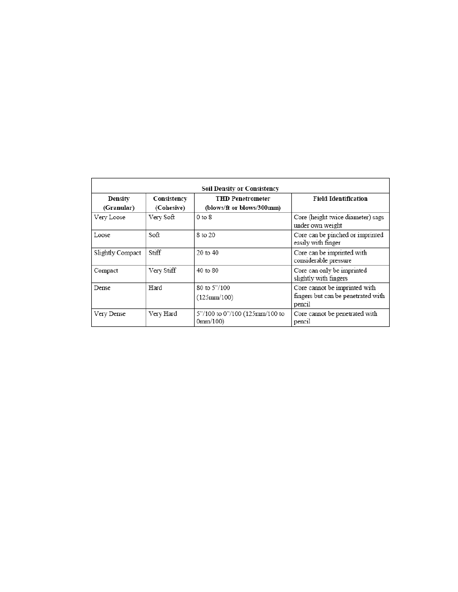
Table 2.1. TxDOT Soil Density and Bedrock Hardness Classification. ............................. 6
Table 2.2. Recommended u
h
/
σ
Values (Dobak 2003). .................................................... 16
Table 2.3. Conditions for 1-D Consolidation Tests (Dobak 2003). .................................. 18
Table 2.4. Summary of Soft Soil Data. ............................................................................. 27
Table 3.1. Summary Information on the Four Selected Embankments. ........................... 45
Table 3.2. Laboratory Test and Field Tests Results (Borehole 99-1a). ............................ 47
Table 3.3. Summary of Consolidation Parameters Used for the Settlement
Estimation. ............................................................................................................ 50
Table 3.4. Summary Table of the Stress Increase in the Soil Mass (Project 1). ............... 52
Table 3.5. Laboratory and Field Tests Results (Boring O-1) (Project 2). ........................ 60
Table 3.6. Laboratory and Field Tests Results (Boring O-4) (Project 2). ........................ 61
Table 3.7. Laboratory and Field Tests Results (Boring O-5) (Project 2). ........................ 62
Table 3.8. Laboratory and Field Tests Results (Boring O-6) (Project 2). ........................ 62
Table 3.9. Summary Table of Consolidation Parameters Used for the Settlement
Estimation (Project 2). .......................................................................................... 65
Table 3.10. Summary Table of the Stress Increase in the Soil Mass. ............................... 67
Table 3.11. Field Test Results (Borings CCB-2, CCB-1, CCR-2, CCR-4 and
CCR-3). ................................................................................................................. 77
Table 3.12. Variation of Soil Types in Five Borings (Project 3). ..................................... 78
Table 3.13. Variation of Moisture Content in the Six Borings (Project 3). ...................... 78
Table 3.14. Variation of Undrained Shear Strength with Depth in the Six Borings
(Project 3).............................................................................................................. 79
Table 3.15. Consolidation Parameters Used for the Settlement Estimation
(Project 3).............................................................................................................. 80
Table 3.16. Summary Stress Increase in the Soil Mass (Project 3). ................................. 83
Table 3.17. Summary of Stress Increase in the Soil Mass. ............................................... 96
Table 4.1. Summary of the Samples Collected. .............................................................. 104
Table 4.2. Summary of Soil Type Parameters (SH3). .................................................... 112
Table 4.3. Summary of Strength Parameters (SH3). ..................................................... 112
Table 4.4. Summary of Consolidation Parameters (SH3). .............................................. 113
xxiii

Table 4-5. Consolidation Parameters from IL Consolidation Tests for NASA
Rd. 1. ................................................................................................................... 117
Table 4-6. Soil Parameters of the Samples Used for Consolidation Tests with
Multiple Loops. ................................................................................................... 118
Table 4.7. Estimated Preconsolidation Pressure. ............................................................ 122
Table 4.8. Summary Table of Compression Indices for Various Clay Soils (Holtz
and Kovacs 1981). .............................................................................................. 125
Table 4.9. Correlations for C
c
(Azzouz et al. (1976); Holtz and Kovacs (1981)). ......... 129
Table 4.10. Summary of Compressibility Parameters for the Clay Soils (SH3
Bridge at Clear Creek). ....................................................................................... 135
xxiv

1
1. INTRODUCTION
1.1. General
Embankments are among the most ancient forms of construction but also have the
most engineering challenges in design, construction, and maintenance. Economic and
social development has brought a considerable increase in the construction of
embankments since the middle of the nineteenth century, particularly since the 1950s
(Leroueil et al. 1990). Embankments are required in the construction of roads,
motorways, and railway networks (elevated embankments, access embankments, and
embankments across valleys), in hydroelectric schemes (dams and retention dikes), in
irrigations and flood control work (regulation dams), harbor installations (seawalls and
breakwaters), and airports (runways) (Leroueil 1994).
Historically, embankments have been placed on sites of good geotechnical
properties in order to reduce the costs associated with their construction. However, during
the last two decades, the demand for expanding the civil infrastructure has forced the use
of sites with soft and compressible soils. It is often found that the regions of densest
population are in the coastal or delta regions covered with recent deposits of clays, mud,
and compressible silts. Therefore, in the past several decades, embankments have been
constructed on compressible soils resulting in a number of problems.
The estimation of total and rate of settlement of an embankment with good
serviceability is the main design concern of embankments on soft soils. The Terzaghi

2
(1925) 1-D classical method is widely used to estimate the total and rate of settlement,
but it has limitations. Several two- and three-dimensional numerical methods have been
developed to predict embankment behavior on soft soils based on the drainage conditions
of the soft soils. All the design methods require laboratory testing and/or field testing to
determine the parameters to be used. Each parameter can be determined using different
tests, resulting in different values for the consolidation parameters (Wissa et al. 1971).
The issues along the Texas Gulf coast are even more complicated by the deltaic nature of
the soft soils and large variability of properties (Vipulanandan et al. 2007 and 2008).
Overestimation of settlement on overconsolidated soft clays may require ground
improvement before construction with added delay and cost to a project. Since the soft
soil shear strength is low, the structures on the soft soils are generally designed so that the
increase in the stress is relatively small and the total stress in the ground will be close to
the preconsolidation pressure. Hence there is a need to investigate methods to better
predict the settlement of embankments on soft soils. Therefore, the recompression index
determined from a consolidation test has more importance in estimating the settlement.
Although the recompression index has been quantified in the literature, its determination
is not clearly defined, especially when there is a hysteretic unloading loop for the soft
clay soil. Also the influence of the unloading stress level on the recompression index is
not clearly quantified.
Instrumenting the embankment with displacement sensors and piezometers to
monitor the field behavior of an embankment on soft soil and comparing the results with
the predicted behavior is the way to validate the accuracy and reliability of settlement and

3
rate of settlement estimation methods or models (Ladd et al. 1994; Vipulanandan et al.
2008).
1.2. Objectives
The overall goal of this study was to review and verify the applicability of
conventional methods used to predict the total amount of and rate of settlement of
embankments on soft clay soils. The specific objectives were as follows:
1) Investigate the methods used by the Texas Department of Transportation
(TxDOT) to estimate the total and rate of settlements of embankments on soft
soils.
2) Verify the predicted settlements with field studies by instrumenting selected
embankments on soft soils. Critically review the selection of the consolidation
parameter to predict the settlement.
3) Analyze the field measurements to verify the applicability of the classical
consolidation theory and recommend methods to further improve the predictions.
1.3. Organization
Chapter 2 summarizes the background information on total and rate of settlement
estimations of embankment on soft clay soils. It also describes the behavior of the soft
soil in the Houston and Galveston areas. Chapter 3 investigates the Texas Department of
Transportation (TxDOT) approaches to predict the total and rate of settlement in
embankments on soft soils. A total of four projects were reviewed and analyzed.
Chapter 4 summarizes the laboratory tests performed and investigates the selection of the

4
settlement parameters to predict the total and rate of settlement. In Chapter 5, field
studies on two instrumented embankments on soft soil are analyzed. Conclusions and
recommendations are given in Chapter 6.

5
2.
SOFT SOILS AND HIGHWAY EMBANKMENT
2.1. General
The decades-long challenge of estimating settlement of embankments on soft clay
soil using laboratory test data and simple consolidation theory has led to either over
predicting or under predicting the total rate of settlement of embankments on soft soils
(Leroueil et al. 1990). Terzaghi (1925) introduced the first known complete solution of
soft clay soil consolidation. His 1-D consolidation theory for settlement calculation and
incremental load (IL) consolidation test (ASTM D 2435) have been widely used because
of their simplicity in predicting the total and rate of settlement of embankments on soft
clay soils. However, due to the time factor imposed by the IL consolidation test
procedure, other consolidation tests such as the constant rate of strain (CRS)
consolidation test (ASTM D 4186), and the constant rate of loading (CRL) test, which are
much faster, were introduced later (Wissa et al. 1971).
2.2.
Soft Clay Soil Definition
As defined by the Unified Soil Classification System (USCS), clays are fine-
grained soils, meaning they have more than 50% passing the No. 200 sieve, and they are
different from the silt soils based on their liquid limit and plasticity index (Holtz and
Kovacs 1981).
Terzaghi and Peck (1967) established that the consistency of a clay can be
described by its compressive strength (q
u
) or by its undrained shear strength S
u
(= q
u
/2)
6
and is regarded as very soft if unconfined compressive strength is less than 3.5 psi
(25 kPa) and as soft soil when the strength is in the range of 3.5 to 7 psi (25 to 50 kPa).
TxDOT identifies a clay soil as soft when the number of Texas Cone
Penetrometer (TCP) blow count is less than or equal to 20 for 1-ft penetration (N
TCP
≤ 20)
(Table 2.1).
Table 2.1. TxDOT Soil Density and Bedrock Hardness Classification.
2.3.
Embankment Settlement
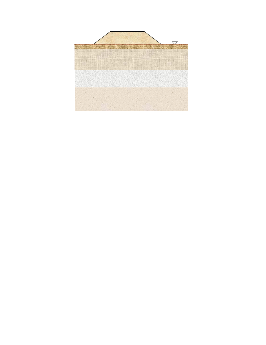
An embankment increases the stress in the soil layers underneath (Fig. 2.1), and
the saturated soft clay soils, being a highly compressible soil, will consolidate (settle).
7
GL
saturated soft clay
sand layer
saturated soft clay
crust
Embankment
GL
saturated soft clay
sand layer
saturated soft clay
crust
Embankment
Fig. 2.1. Typical Configuration of Soil Layers under an Embankment.
2.3.1. Terzaghi Classical 1-D consolidation model
Terzaghi’s complete solution for one-dimensional consolidation is stated as
follows (Leroueil et al. 1990):
Hypotheses:
(1) The strains in the clay layer are 1-D and remain small (
ε
z
is small).
(2) The soil is homogeneous and saturated.
(3) The particles of the soil and the pore fluid are incompressible.
(4) The flow of the pore fluid is 1-D and obeys Darcy’s law.
(5) The permeability is constant (k = constant).
(6) A linear relation exists between the effective vertical stress (
σ’
v
) and the void
ratio
de = -a
v
d
σ’
v
. 2-1
(7) The soil has no structural viscosity.

8
The use of the first hypothesis permits the fundamental equation of consolidation
to be written in the form
(
)
2
2
w
o
z
u
e
1
k
t
e
∂
∂
+
=
∂
∂
γ
2-2
where e is void ratio, e
o
is initial void ratio, k is coefficient of permeability,
γ
w
is unit
weight of water, t is time, u is pore water pressure, and z is drainage path
.
This equation expresses the fact that the rate of change in void ratio (and, as a
result, the rate of deformation) at a given instant depends on the permeability and the
form of the excess pore pressure isochrones, but not on the compressibility of the
material.
Using hypotheses (6) and (7), Equation 2-2 can be written
(
)
2
2
1
z
u
a
e
k
t
t
u
v
w
o
v
∂
∂
+
=
∂
∂
−
∂
∂
γ
σ
. 2-3
When the applied stress
'
v
σ is constant (
0
=
∂
∂
t
v
σ
), Equation 2-3 takes the classical form
of the Terzaghi equation
(
)
2
2
v
w
o
z
u
a
e
1
k
t
u
∂
∂
+
=
∂
∂
γ
. 2-4
The function
(
)
w
w
o
a
/
e
1
k
γ
+
in this differential equation has been called the
coefficient of consolidation (
v
c ) and is given by

9
v
w
o
v
w
v
m
k
e
a
k
c
γ
γ
=
⎟⎟
⎠
⎞
⎜⎜
⎝
⎛
+
=
1
2-5
and
2
2
z
u
c
t
u
v
∂
∂
=
∂
∂
. 2-6
This equation can also be written in terms of excess pore pressures (Schlosser et
al. 1985)
2
2
)
(
)
(
z
u
c
t
u
v
∂
Δ
∂
=
∂
Δ
∂
. 2-7
Equation 2-6 is the basic differential equation of Terzaghi’s consolidation theory
and is solved with the following boundary conditions:
0
,
0
0
,
2
0
,
0
u
u
t
u
H
z
u
z
dr
=
=
=
=
=
=
giving the time factor T
v
as follows
2
dr
v
v
H
t
c
T
=
. 2-8
For the given load increment on a specimen, Casagrande and Fadum (1940)
developed the graphical logarithm-of-time method to determine c
v
at 50% average degree
of consolidation with T
50
= 0.197. Taylor (1942) developed the square-root-of-time
graphical method giving c
v
at 90% average of consolidation with T
90
= 0.848. These two
graphical methods, Equations 2-9 and 2-10, are commonly used to determine the
coefficient of consolidation and are described in ASTM D 2435 – 96.

10
Using the Casagrande method,
50
2
197
.
0
t
H
c
dr
v
=
2-9
and using the Taylor method,
90
2
848
.
0
t
H
c
dr
v
=
2-10
where H
dr
is the maximum drainage path.
The primary consolidation settlement (S
p
) of the clay is represented as follows:
For normally consolidated clay
⎟
⎟
⎠
⎞
⎜
⎜
⎝
⎛
+
+
=
'
0
'
'
0
0
c
p
log
e
1
H
C
S
σ
σ
Δ
σ
2-11
and for overconsolidated clay
⎟
⎟
⎠
⎞
⎜
⎜
⎝
⎛
+
+
+
⎟
⎟
⎠
⎞
⎜
⎜
⎝
⎛
+
=
p
'
'
0
0
c
'
0
p
0
r
p
log
e
1
H
C
log
e
1
H
C
S
σ
σ
Δ
σ
σ
σ
2-12
where
C
c
= compression
index
C
r
= recompression
index
e
o
= initial void ratio
H
= soil layer height
Δσ
'
σ
'
o
= in-situ vertical effective stress at rest
σ
p
= preconsolidation
pressure
Δσ
'
= stress increase in the soil mass due to embankment loading.

11
(1)
The time rate of consolidation
From the incremental load (IL) test
t
H
T
c
H
t
c
T
2
dr
v
v
2
dr
v
v
=
→
=
2-13
and from the Constant rate of strain (CRS) test (Wissa et al. 1971)
⎥
⎦
⎤
⎢
⎣
⎡
−
⎥
⎦
⎤
⎢
⎣
⎡
−
=
v
h
1
v
2
v
2
v
u
1
log
t
2
log
H
c
σ
Δ
σ
σ
2-14
where
c
v
=
coefficient of consolidation
H
dr
=
longest drainage path
H
=
average specimen height between t
1
and t
2
T
v
=
time factor
u
h
=
average excess pore pressure between t
2
and t
1
Δ
t
=
elapsed time between t
1
and t
2
σ
v1
=
applied axial stress at time t
1
σ
v2
=
applied axial stress at time t
2.
The following are the standard definitions and methods of determination for all
the parameters used in Equations 2-11, 2-12, 2-13, and 2-14.
12
2.3.2. Incremental Load (IL) test (ASTM D 2435)
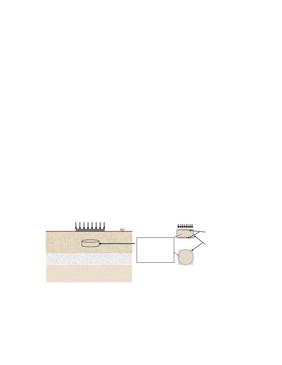
The one-dimensional consolidation test procedure, a simulation of the field
condition in the laboratory (Fig. 2.2) first suggested by Terzaghi to determine the
compressibility parameters and rate of settlement of clayey soils, is performed in a
consolidometer, also called the oedometer. Following the standard test method for 1-D
consolidation (American Society of Testing and Material (ASTM) D 2435 – 96), the soil
specimen is placed inside a metal ring with two porous stones, one at the top of the
specimen and another at the bottom (Fig. 2.2) to comply with the plain strain condition.
Load increment ratios of unity are applied, and each increment is left on for 24 hours to
obtain characteristic time-settlement relationships, from which consolidation parameters
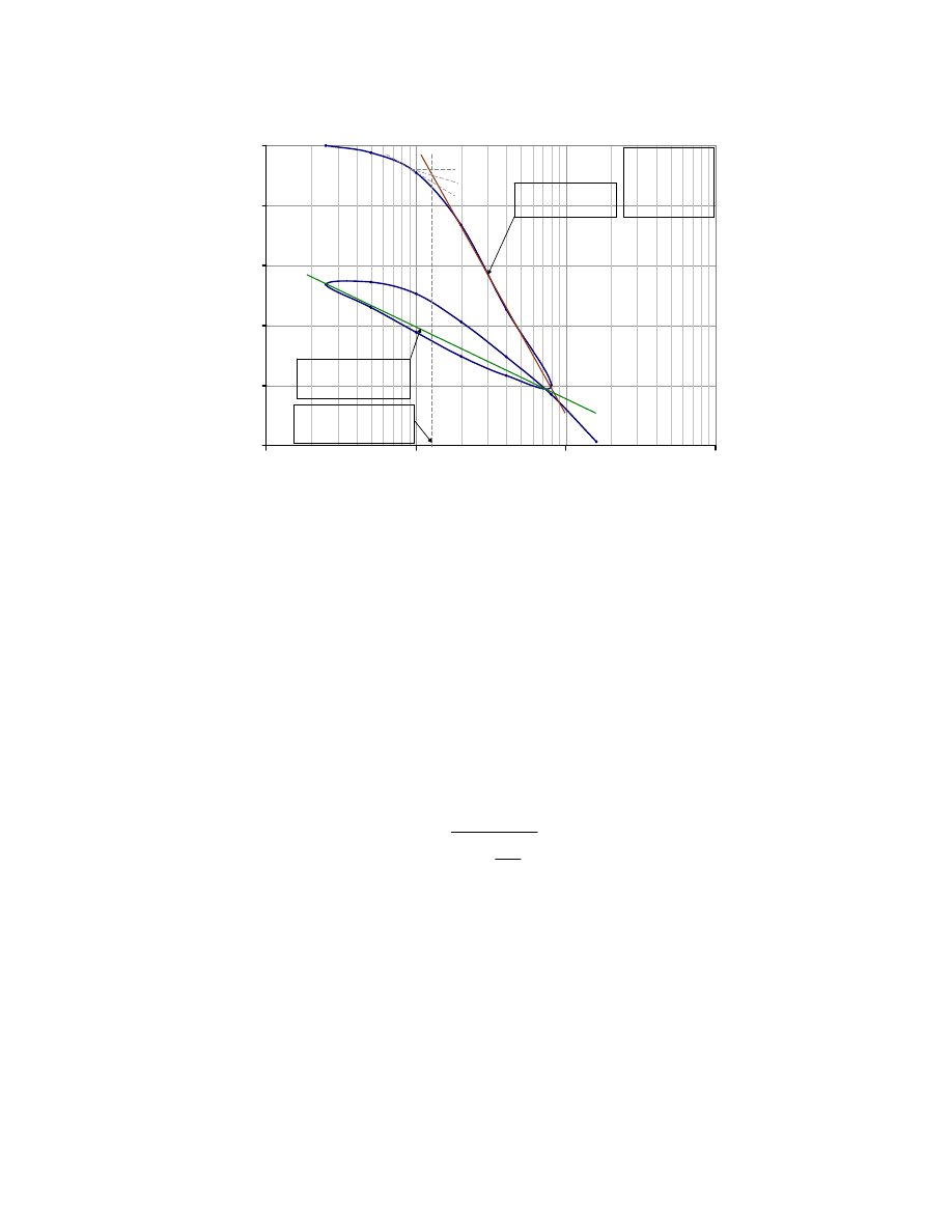
are obtained. From the void ratio (e) versus logarithm of vertical stress (log
σ
v,
)
(Fig. 2.3)
relationship, the preconsolidation pressure
σ
p
, the compression index C
c
, and
recompression index C
r
are determined. The specimen is kept under water during the test.
The test takes several days (typically from 5 to 15 days or more).
Fig. 2.2. Field Condition Simulation in Laboratory Consolidation Test.
Lab
Field
metal ring
(consolidometer)
Porous stone
Applied load
saturated soft
clay
saturated soft clay
GL
Soil Specimen
Φ = 2.5 in.
H = 0.71 in.–1 in.
External load
sand layer
13
0.60
0.70
0.80
0.90
1.00
1.10
0.1
1.0
10.0
100.0
Vertical effective stress
σ'
(tsf)
Vo
id
r
at
io
e
e
o
= 1.10
σ
p
= 1.36 tsf
C
c
= 0.443
Cr = 0.117
1
5
3
2
6
4
σ
p
:
the preconsolidation
pressure
Slope of this line is
C
c
the compression index
Slope of this line is
C
r
the recompression index
Fig. 2.3. Typical e – log
σ
v
Relationship for Overconsolidated Clay.
The preconsolidation pressure,
σ
p
, is the highest stress the clay soil ever felt in its
history. There are several methods to determine
σ
p
, which are discussed in Chapter 4, but
the Casagrande graphical method was used in Fig. 2.3.
The compression index, C
c
, is the slope of the virgin compression section of the
curve (Section 3 – 4 in Fig. 2.3)
3
4
3
4
c
log
)
e
e
(
C
σ
σ
−
−
=
. 2-15
The recompression index C
r
is the average slope of the hysteretic loop, as shown
in Fig. 2.3, and it is assumed to be independent of the stress.

14
2.3.3. Constant rate of strain test
In 1969, after about 40 years of use of the IL test without major modification for
clay soil compressibility and rate of settlement parameter determination, two new
methods of performing a consolidation test were introduced:
- the Controlled Gradient test (CG test) by Lowe et al. (1969), and
- the Constant Rate of Strain test (CRS test) by Smith and Wahls (1969).
These tests were used to overcome some of the limitations of the conventional test
(IL test) in real-time monitoring of pore water pressure (u vs. t) and the total time needed
to complete a test.
The Constant Rate of Strain (CRS) 1-D consolidation, also specified as
Controlled-Strain Loading by ASTM D 4186-86, is the technique in which a saturated
clay sample is consolidated at constant volume under a back pressure and loaded, with no
lateral strain, by incremental load, at a constant rate of strain (Wissa et al. 1971).
Terzaghi’s complete solution for 1-D consolidation and its hypotheses are valid and
applied.
The features of the CRS consolidation test are as follows:
- contrary to the oedometer cell, the sample is provided only one drainage
surface, the top porous stone; the bottom drainage surface is locked and used
to measure the excess pore water pressure at the sample base (u
h
) (Fig. 2.4),
- fully computerized because of the need for constant rate of strain (dέ = 0),
which requires a control and update of the stress applied at all times (t)
(Fig 2.5 and Fig. 2.6),

15
- faster compared to the IL test. The CRS test can be completed in less than
24 hours.
The parameters governing the CRS consolidation test (Wissa et al. 1971) and
ASTM D 4186-86, are as follows:
- consolidation test results are strain rate (
ε
&
) dependent,
- selection of strain rate is based on the criteria developed by Wissa et al.
(1971). The strain rate (
ε
&
) does not affect as much the e – log
v
σ
curve as
the coefficient of consolidation c
v
. Consequently, the optimum rate of strain
for a given soil is a trade-off between the speeds best suited for determining
the e – log
v
σ
curve and the coefficient of consolidation c
v
(
v
σ
is the average effective stress), and
- because field strain rates cannot be accurately determined or predicted, it is
not feasible to relate the laboratory-test strain rates to the field strain rates.
However, it may be feasible to relate field pore pressure ratios (u
h
/
σ
v
) to
laboratory pore pressure ratios. After Wissa et al. (1971), all parameters can
be accurately determined with the strain rate giving u
h
/
σ
v
values of 2% to 5%,
but the ASTM D 4186-86 established a preferable ranging from 3% to 30%.
As summarized by the compiled data of Dobak (2003) (Table 2.2), the range of
pore pressure ratios for a representative test providing reliable coefficient of
consolidation (c
v
) depends on the type of the soil.
16
Table 2.2. Recommended u
h
/
σ
Values (Dobak 2003).
Recommended
u
h
/σ values
Soil type
Reference
0.5 Kaolinites,
Ca-montmorillonites, Messena clay
Smith and
Wahls (1969)
0.05 Boston
blue
clay
(artificially sedimented)
Wissa et al.
(1971)
0.1-0.15
Bakebol clay
Sällfors (1975)
0.3-0.5
(u
hmin
= 7 kPa)
Silts and clays from the coal field of
Mississippi Plains (Kentucky)
Gorman et al.
(1978)
Note: In the table u
hmin
is u
h
- the coefficient of consolidation, the only parameter differently determined
from the IL parameters, is given by the following relationship:
⎥
⎦
⎤
⎢
⎣
⎡
−
Δ
⎥
⎦
⎤
⎢
⎣
⎡
−
=
v
h
v
v
v
u
t
H
c
σ
σ
σ
1
log
2
log
1
2
2
2-16
where
σ
v1
= applied axial stress at time t
1
σ
v2
= applied axial stress at time t
2
H = average specimen height between t
1
and t
2
Δt = elapsed time between t
1
and t
2
u
h
= average excess pore pressure between t
2
and t
1
σ
v
= average total applied axial stress between t
2
and t
1
.
17
Fig. 2.4. Constant Rate of Strain (CRS) Consolidation Cell Used at the
University of Houston (GEOTAC Company 2006).
Fig. 2.5. Schematic of CRS Test Frame Used at the University of Houston
(GEOTAC Company 2006).
18
Fig. 2.6. Commercially Available CRS Test System (GEOTAC Company 2006).
Table 2.3. Conditions for 1-D Consolidation Tests (Dobak 2003).
Conditions of loading
Exponential model of
stress changes
σ
= a . t
n
Governing physical processes
σ = const
n = 0
- creep of soil skeleton
- seepage
CRL
Δσ/Δt = const
n = 1
CRS
CG
Δσ/Δt increasing
n > 1
IL
- character and changes in stress
increase
- seepage
- creep of soil skeleton
CL
Types of tests
CRL is the Constant Rate of Loading test.
CG is the Constant Gradient test, meaning that the pore water pressure at the base of the specimen is kept
constant throughout the test.

19
2.3.4. Two-dimensional consolidation
Consolidation under an embankment is actually two- or three-dimensional.
Several theoretical solutions for the two-dimensional consolidation problem were
developed as early as 1978 (Leroueil et al. 1990); these have certain deficiencies in their
hypotheses upon which they are based:
(1) Isotropic behavior of the clay skeleton.
(2) Constant coefficient of consolidation.
(3) Determination of consolidation parameters in the horizontal direction.
The effect of the second dimension is only important when the width of the base
(W) of the embankment is less than twice the thickness (W < 2d) of the clay layer
(Leroueil et al. 1990).
The use of these 2-D consolidation models was uncommon until the recent
development and popularization of finite element (FE) and finite difference (FD)
computer programs. In fact, the need to combine stability analysis with settlement
analysis resulted in 2-D and 3-D numerical modeling of the problem (FE and FD).
To truly understand and predict soils’ behavior, it is necessary to have a complete
knowledge of stresses and strains at all compatible loading levels right up to failure.
Constitutive relations or stress-strain laws embrace information on both shear stresses
and deformations at all stages of loading, from pre-failure states to failure (Nagaraj and
Miura 2001).
Consequently, several 2-D constitutive models for soft clay soil behavior have
been developed and implemented in FE and FD programs. For example, linearly elastic,
perfectly plastic, hyperbolic, and several other academic models were implemented in the
20
existing numerical frames (Plaxis, FLAC). Most of the models are isotropic, but soft clay
soil is an anisotropic material. Models such as MIT-E3 (Whittle and Kavvadas 1994) and
the multi-laminate model (Cudny 2003) are two of the advanced models that considered
the anisotropic behavior of soft clay soil. All these models require several parameters,
leading to more laboratory testing.
2.3.5.
Stress increase in the soil mass due to embankment loading (
Δσ)
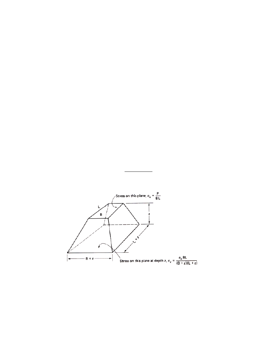
• 2:1 Method
The 2:1 method is the simplest method to calculate the stress increase with depth,
due to embankment loading, in the soil mass. It is an empirical method (Holtz and
Kovacs 1981) based on the assumption that the area over which the load acts increases in
a systematic way with depth, Fig. 2.7.
(
)(
)
z
L
z
B
BL
o
z
+
+
=
σ
σ
Δ
2-17
Fig. 2.7. 2:1 Method for Vertical Stress Distribution (Holtz and Kovacs 1981).
21
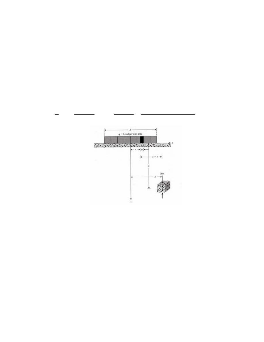
• Modified Boussinessq method
The vertical stress caused by a vertical strip load (finite width and infinite length)
(Fig. 2.8) is given by Equation 2-18, which is derived from the Boussinessq (1883)
solution of stresses produced at any point in a homogeneous, elastic, and isotropic
medium as the result of a point load applied on the surface of an infinitely large half-
space.
(
)
[
]
[
]
⎪⎭
⎪
⎬
⎫
⎪⎩
⎪
⎨
⎧
+
−
+
−
−
−
⎥
⎦
⎤
⎢
⎣
⎡
+
−
⎥
⎦
⎤
⎢
⎣
⎡
−
=
Δ
−
−
2
2
2
2
2
2
2
2
1
1
)
4
/
(
)
4
/
(
2
/
tan
)
2
/
(
tan
z
B
B
z
x
B
z
x
Bz
B
x
z
B
x
z
q
z
π
σ
2-18
Fig. 2.8. Vertical Stress Due to a Flexible Strip Load (Das 2006).
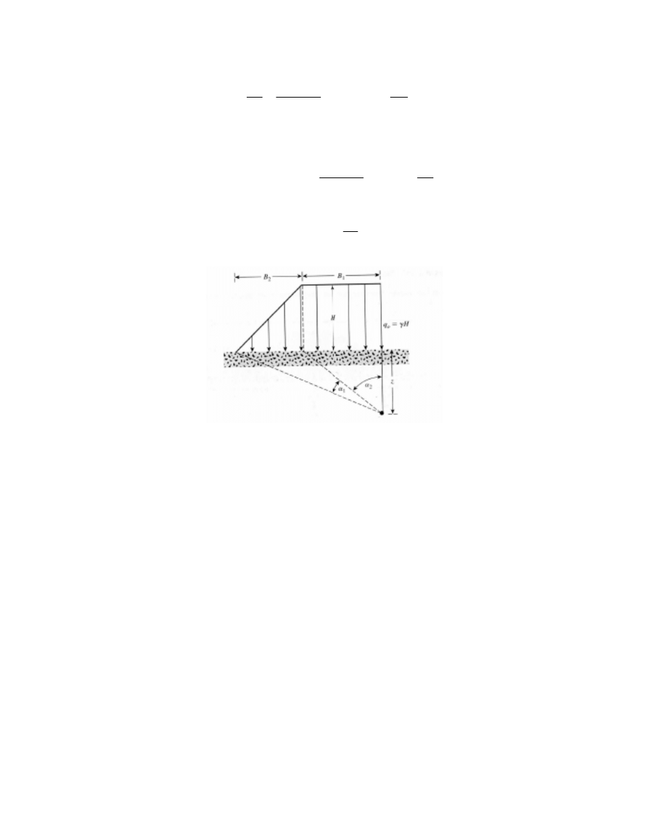
• Osterberg method
Based on Boussinessq’s expression, Osterberg derived the vertical stress increase
in a soil mass due to an embankment loading, considering its real geometry (crest)
(Fig. 2.9), which is given by the following equations:
22
(
)
( )
⎥
⎦
⎤
⎢
⎣
⎡
−
+
⎟⎟
⎠
⎞
⎜⎜
⎝
⎛
+
=
2
2
1
2
1
2
2
1
o
z
B
B
B
B
B
q
α
α
α
π
σ
Δ
2-19
where
H
q
γ
=
0
⎟
⎠
⎞
⎜
⎝
⎛
−
⎟
⎠
⎞
⎜
⎝
⎛
+
=
−
−
z
B
tan
z
B
B
tan
)
radian
(
1
1
2
1
1
1
α
2-20
⎟
⎠
⎞
⎜
⎝
⎛
=
−
z
B
tan
1
1
2
α
. 2-21
Fig. 2.9. Embankment Loading Using Osterberg’s Method (Das 2006).
2.3.6. Summary and discussion
Terzaghi’s (1925) 1-D consolidation theory is the basis for consolidation
settlement estimation tests. CRS, CRL, and CG tests have been created to account for
some of the limitations of the IL test.
2-D and 3-D consolidation models have been developed based on the real
behavior of soft soil under embankments. This has resulted in more advanced settlement
calculation and avoidance of the oversimplification of the settlement problem.

23
Settlement issues such as effective stress increase, estimation of soil properties,
drainage conditions, and soil layering are considered as critical for more accurate
prediction of the total amount of and rate of settlement.
2.4.
Behavior of Marine and Deltaic Soft Clays
More and more construction projects are encountering soft clays, and hence, there
is a need to better quantify the properties of soft clays. In this study, data from many parts
of the world are used to characterize the soft clays based on the type of deposits.
Physical, index, and strength properties for marine and deltaic soft clays were determined
and investigated using the soft soil database developed from the published data in the
literature. Data were analyzed using statistical methods (mean, standard deviation,
variance, and probability density function), and the undrained shear strength (S
u
) versus
preconsolidation (
σ
p
) was verified. A new strength relationship between undrained shear
strength (S
u
) and in-situ vertical stress (
σ
v
) has been developed for the soft clays. Also,
constitutive models used for soft soil behavior prediction have been reviewed.
Soft clays are found in marine, lacustrine, deltaic, and coastal regions or as a
combination of deposits around the world. They are of relatively recent geological origin,
having been formed since the last phase of the Pleistocene, during the past 20,000 years.
In addition to the geological factors, salinity, temperature, and the type of clay have a
direct effect on the lithology of the soft clays. The behavior of soft soils has been studied
for well over four decades, and there are several property relationships in the literature on
soft clays.

24
Bjerrum (1974) evaluated methods to determine the undrained shear strength of
soft clay soils. Based on the study, it was concluded that the laboratory triaxial tests on
undisturbed samples consolidated to in-situ effective stress better represented the strength
of the soft soil in different directions. It was also noted that the field vane test is the best
possible practical approach for determining the undrained strength for stability analysis.
A number of studies after Bjerrum (1974) have attempted to relate the undrained shear
strength of soil to the preconsolidation pressure (
σ
p
), in-situ vertical stress (
σ
v
), time-to-
failure, and plasticity index (PI). Since the early 1970s, a number of investigators have
studied the behavior of soft soils and their properties have been documented in the
literature.
2.4.1. Soil correlations
Comprehensive characterization of soft soil at a particular site would require an
elaborate and costly testing program generally limited by funding and time. Instead, the
design engineer must rely upon more limited soil information and that is when
correlations become most useful. However, caution must always be exercised when using
broad, generalized correlations of index parameters or in-situ test results with soft soil
properties. The source, extent, and limitations of each correlation should be examined
carefully before use to ensure that extrapolation is not being done beyond the original
boundary conditions. In general, local calibrations, where available, are to be preferred
over broad, generalized correlations. In this study, information reported from various
locations around the world was used to develop statistical geotechnical properties and
correlations. In addition, some of the common correlations in the literature will be

25
verified with the data available. The correlations in the literature will be helpful in
identifying the important variable and in eliminating the others.
Soft soil is a complex engineering material that has been formed by a combination
of various geologic, environmental, and chemical processes. Because of these natural
processes, all soil properties in-situ will vary vertically and horizontally. Recovering
undisturbed soil samples is considered a challenge and various methods are being
adopted around the world. Even under the most controlled laboratory test conditions, soil
properties will exhibit variability. The property variability is notable in samples
recovered from shallow depths considered being in the Active Zone. Although property
in-situ condition correlations are important to a better understanding of the factors
influencing the behavior of soft clays, adequate precautions must be taken to verify the
relationships for more specific applications.
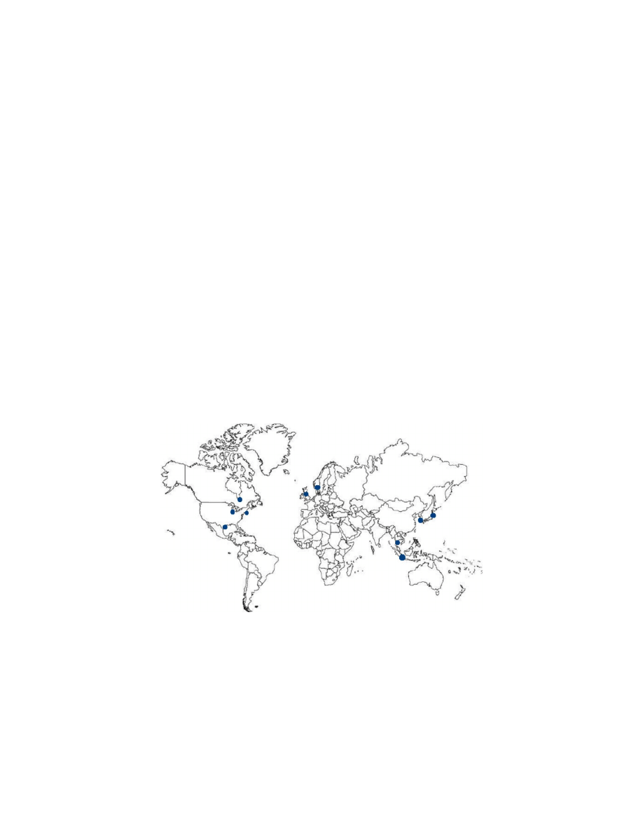
2.4.2. Database on soft soils
Soft clays are encountered around the world (Fig. 2.10), and the information in
the literature can be characterized based on the type of deposits. In general, the properties
of the soft soils will be influenced by the geology, mineralogy, geochemistry, and the
lithology (composition and soil texture) of the deposits. Although a number of physical
and chemical factors enter into the classifications of deposits, in the geotechnical
literature, classification is made according to the marine, lacustrine, coastal, or deltaic
depositional environments. Marine clays are the most investigated group of soft clays and
are generally characterized as homogenous deposits with flocculation of particles due to
salinity resulting in highly sensitive clays. Soft clay soils data from Japan (Ariake clay),
South Korea (Pusan clay), Norway (Drammen, Skoger Spare, Konnerud, and Scheitlies
26
clays), Canada (Eastern Canada clay), and the USA (Boston blue clay) are classified as
marine deposits. Properties of the soft soils collected from the literature are summarized
in Table 2.4. A total of 52 data sets were collected on marine clays from around the
world. The rate of deposition varied from 30 to 1600 cm/1,000 years and is compared to
other deposits in Fig. 2.11.
The soft soils from the Houston-Galveston area in Texas, U.S.A., are
characterized as deltaic deposits. The deltas of large rivers form a very active and very
complex sedimentation environment. Deltaic deposits are generally stratified in a random
manner with the interbedded coarse materials, organic debris, and shells. The
combination of a significant amount of solid material, topography, and current, along
with the interaction between fresh river water and salt seawater, led to high rates of
deltaic deposits (Fig. 2.11).
Fig. 2.10. Locations of Soft Clay Soils Used for the Analysis.
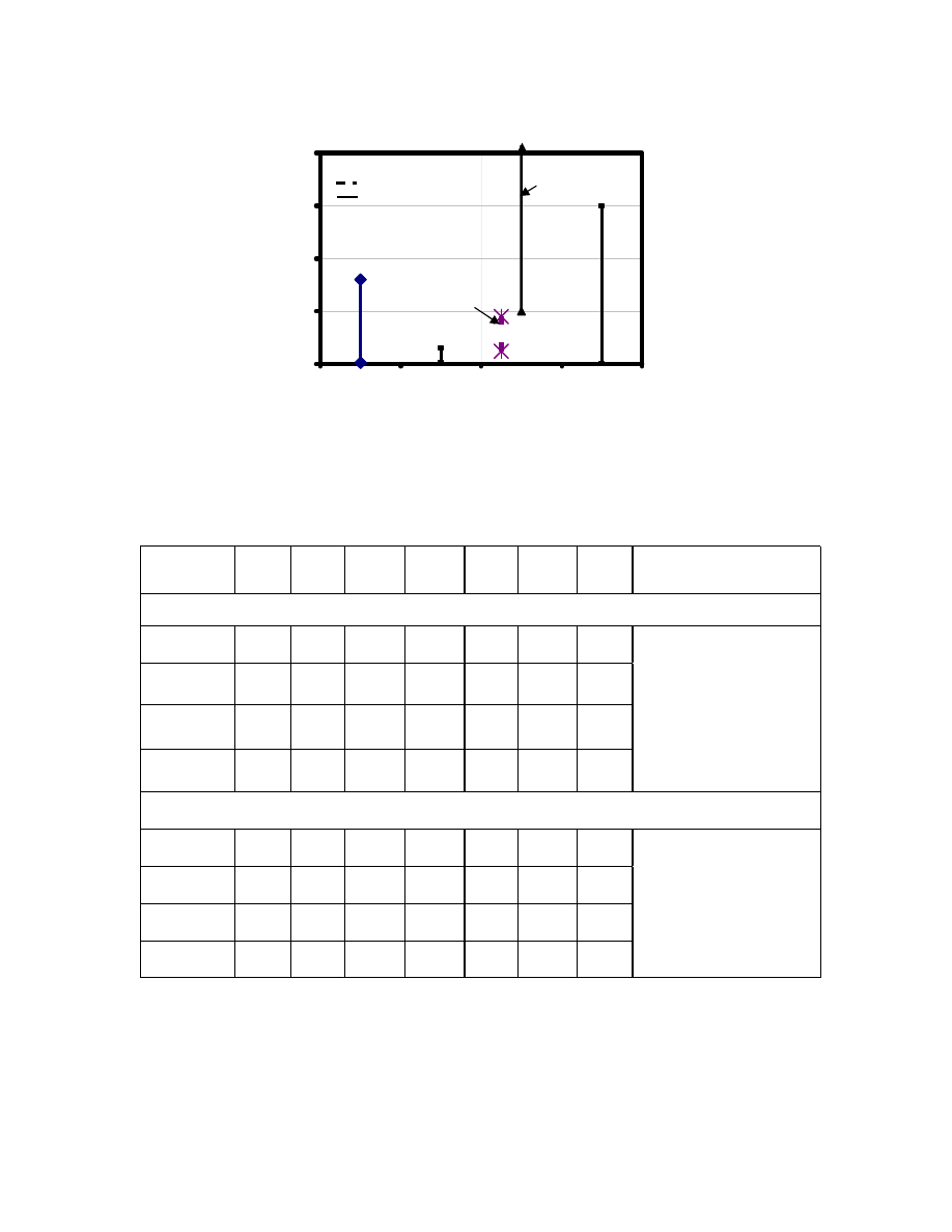
27
0
1000
2000
3000
4000
0
1
2
3
4
TYPE OF CLAY
D
epos
it
ion rat
e (
cm
/ 1000
years
)
MARINE
COASTAL
LACUSTRINE
DELTAIC
the deltaic deposition
rate ends at 30000
Houston &
Galveston
Vipulanandan et al. 2007
Leroueil et al. 1990
Fig. 2.11. Rate of Sedimentation of Different Types of Clay Deposits
(Leroueil 1990).
Table 2.4. Summary of Soft Soil Data.
W
n
(%)
W
L
(%)
PL
(%)
PI
(%)
S
u
(kPa)
σ
p
(kPa)
e
o
(%)
References
30 - 133 32 -121 19.4 - 33 12 - 50.5 1.8 - 25 7.5 - 248 80 -352
73.6
64.2
24.3
35.2
17.5
74.5
195.2
22.3
22.2
3.4
11.7
6.6
41.8
58.9
30.3
34.6
13.8
33.2
37.9
56.1
30.2
13 - 59
24 - 93
8 - 35
8 - 61
7 - 25
-
34 - 156
28.9
53.6
21.8
32.4
19.5
-
76.7
9.5
22.7
6.9
16.9
5.1
-
25.1
32.8
42.4
31.6
52.2
26.2
-
32.7
ANALYSIS
Nagaraj & Miura (2001); Chung et al.(2002);
Shibuya & Tamrakar (1999);
Nash, Sills, Davison, Powell & Lloyd (1992)
Vipulanandan et al (2006)
RANGE
DELTAIC CLAY : Houston_Galveston (Number of data sets = 97)
MARINE CLAY (Number of data = 51)
RANGE
COV (%)
COV (%)
MEAN
STANDARD
DEVIATION
MEAN
STANDARD
DEVIATION

28
Houston and Galveston, Texas, are on two Pleistocene terrace formations found
along the Gulf Coast, west of the Mississippi River and north of the Rio Grande River,
exposed at the surface to about 100 km inland from the present coastline. The lower
formation, termed the upper Lissie formation or the Montgomery formation (the latter
designation will be used here), was deposited on a gentle slope on an older Pleistocene
formation during the Sangamon Interglacial Stage by streams and rivers near the existing
coast where numerous large and small rivers deltas developed. After deposition, the
nearby sea level was lowered during the first Wisconsin Glacial Stage, producing
desiccation and consolidation of the Montgomery soils, which consisted primarily of
clays and silts. At the beginning of the Peorian Interglacial Stage as the glaciers were
retreating, the sea level returned to its previous level, producing a preconsolidation effect
within the Montgomery formation. At the same time, rivers and streams produced
sedimentary deposits on top of the slightly seaward-sloping Montgomery formation from
the existing coastline to about 60 km inland. The resulting new formation, primarily a
fresh-water deposit sloping toward the Gulf of Mexico, has characteristics typical of
deltaic environments, including point bar, natural levee, backswamp, and pro-delta
deposits within, beside, and at the termination of distributary channels. This formation is
known as the Beaumont formation in Texas. After deposition, the nearby Gulf of Mexico
receded by about 125 m once more during the late Wisconsin Glacial Stage, inducing
desiccation in the Beaumont and redesiccating the underlying Montgomery. Finally, with
the recession of the late Wisconsin glaciers, the sea level returned to its present level,
leaving both formations preconsolidated through desiccation. The rate of deposit was

29
estimated to be between 250-900 cm/1,000 years (Vipulanandan et al. 2007). A total of
97 data sets have been collected from Houston and Galveston area deltaic soil, and the
range of values is summarized in Table 2.4.
2.4.3. Statistical Properties
(a) Marine Clay
(i) Natural Moisture Content (W
n
): The moisture content varied from 30% to 133%
with a mean of 73.6%, standard deviation of 22.3%, and coefficient of variation of
30.3%. This coefficient of variation was the second lowest observed for the marine clay
properties being investigated in this study. This COV was in the typical range of values
observed for other marine clay properties. Of the probability distribution functions
considered (Beta, Erlang, Exponential, Gamma, Lognormal, Normal, Triangular,
Uniform, and Weibull), the Beta distribution has the least error based on the 51 data sets.
(ii) Liquid Limit (LL): The liquid limit varied from 32% to 121% with a mean of 64.2%,
standard deviation of 22.2%, and coefficient of variation of 34.6%. The variability
observed in the LL, based on the COV, was similar to the moisture content. Of the
probability distribution functions considered (Beta, Erlang, Exponential, Gamma,
Lognormal, Normal, Triangular, Uniform, and Weibull), the Triangular distribution has
the least error, based on the 51 data sets.
(iii) Plasticity Limit (PL): The plastic limit varied from 19.4% to 33% with a mean of
24.3%, standard deviation of 3.4% and coefficient of variation of 13.8%. The variability
observed in the PL, based on the COV, was the lowest, indicating that it had the lowest
variability of all the other marine clay properties being investigated in this study. Of the

30
probability distribution functions considered (Beta, Erlang, Exponential, Gamma,
Lognormal, Normal, Triangular, Uniform, and Weibull), the Normal distribution has the
least error based on the 13 data sets.
(iv) Plasticity Index (PI): The plasticity index varied from 12% to 50.5%, with a mean
of 35.2%, a standard deviation of 11.7%, and a coefficient of variation of 33.2%. Of the
probability distribution functions considered (Beta, Erlang, Exponential, Gamma,
Lognormal, Normal, Triangular, Uniform, and Weibull), the Beta distribution has the
least error, based on the 13 data sets.
(v) Undrained Shear Strength (S
u
): The undrained shear strength varied from 1.8 kPa
to 25 kPa, with a mean of 17.5 kPa, a standard deviation of 6.6 kPa, and a coefficient of
variation of 37.9%. The COV was in the same range as the LL, typical for the marine
clay. Of the probability distribution functions considered (Beta, Erlang, Exponential,
Gamma, Lognormal, Normal, Triangular, Uniform, and Weibull), the Beta distribution
(Fig. 2.12) has the least error, based on the 51 data sets.
(vi) Undrained Shear Strength-to-In situ Stress Ratio (S
u
/
σ
v
): The undrained shear
strength-to-in situ stress ratio varied from 0.08 to 1.39, with a mean of 0.52, a standard
deviation of 0.27, and a coefficient of variation of 51.9%. Of the probability distribution
functions considered (Beta, Erlang, Exponential, Gamma, Lognormal, Normal,
Triangular, Uniform, and Weibull), lognormal distribution has the least error, based on
the 49 data sets.
(vii) Preconsolidation Pressure (
σ
p
): The preconsolidaton pressure varied from 7.5 kPa
to 248 kPa with a mean of 74.5 kPa, a standard deviation of 41.8 kPa, and a coefficient of
variation of 56.1 kPa. Of the probability distribution functions considered (Beta, Erlang,

31
Exponential, Gamma, Lognormal, Normal, Triangular, Uniform, and Weibull), the
Weibull distribution has the least error, based on the 51 data sets.
(viii) Undrained Shear Strength-to-Preconsolidation Pressure Ratio (S
u
/
σ
p
): The
Undrained Shear Strength-to-Preconsolidation Pressure Ratio varied from 0.06 to 0.47,
with a mean of 0.26, a standard deviation of 0.08, and a coefficient of variation of 30.8.
Of the probability distribution functions considered (Beta, Erlang, Exponential, Gamma,
Lognormal, Normal, Triangular, Uniform, and Weibull), the Beta distribution has the
least error, based on the 51 data sets.
(ix) Overconsolidation Ratio (OCR): The overconsolidation ratio varied from 1 to 4,
with a mean of 2.01, a standard deviation of 0.89, and a coefficient of variation of 44.3.
Of the probability distribution functions considered (Beta, Erlang, Exponential, Gamma,
Lognormal, Normal, Triangular, Uniform, and Weibull), the Beta distribution has the
least error, based on the 49 data sets.
(x) Void ratio (e
o
): The void ratio varied from 80% to 352%, with a mean of 195.2%, a
standard deviation of 58.9%, and a coefficient of variation of 30.2%. The COV was in the
same range of several other parameters for the marine clay. Of the probability distribution
functions considered (Beta, Erlang, Exponential, Gamma, Lognormal, Normal,
Triangular, Uniform, and Weibull), the Normal distribution has the least error, based on
the 51 data sets.
(xi) Undrained Shear Strength-to-Void ratio (S
u
/e
o
): Undrained shear strength-to-void
ratio varied from 0.68 to 24.51, with a mean of 10.10, a standard deviation of 5.20, and a
coefficient of variation of 51.5. Of the probability distribution functions considered (Beta,

32
Erlang, Exponential, Gamma, Lognormal, Normal, Triangular, Uniform, and Weibull),
the Normal distribution has the least error based on the 51 data sets.
(b) Deltaic Clay
(i) Natural Moisture Content (W
n
). The moisture content varied from 13% to 59%,
with a mean of 28.9%, a standard deviation of 9.5%, and a coefficient of variation of
32.8%. The probability distribution function was normal based on 97 data. Based on the
mean and range of moisture contents, the moisture content in the deltaic soils were less
than half that of marine clays. Based on variance, the marine clay had a more than 600%
higher variance than did deltaic clay. This large variance could partly be due to the fact
that the marine clay data was gathered from three continents, as compared to the deltaic,
which was from one location. Of the probability distribution functions considered (Beta,
Erlang, Exponential, Gamma, Lognormal, Normal, Triangular, Uniform, and Weibull),
Beta distribution has the least error, based on 97 data.
(ii) Liquid Limit (LL). The liquid limit varied from 24% to 93%, with a mean of 53.6%,
a standard deviation of 22.7%, and a coefficient of variation of 2.36%. Of the probability
distribution functions considered, (Beta, Erlang, Exponential, Gamma, Lognormal,
Normal, Triangular, Uniform, and Weibull), Beta distribution has the least error based on
97 data.
(iii) Plastic Limit (PL). The plastic limit varied from 8 to 35, with a mean of 21.8, a
standard deviation of 6.9, and a coefficient of variation of 31.6%. Of the probability
distribution functions considered (Beta, Erlang, Exponential, Gamma, Lognormal,

33
Normal, Triangular, Uniform, and Weibull), Weibull distribution has the least error,
based on 97 data.
(iv) Plasticity Index (PI). The plasticity index varied from 8 to 61, with a mean of 32.4,
a standard deviation of 16.9, and a coefficient of variation of 52.2%. Of the probability
distribution functions considered (Beta, Erlang, Exponential, Gamma, Lognormal,
Normal, Triangular, Uniform, and Weibull), Beta distribution has the least error, based
on 97 data.
(v) Undrained Shear Strength (S
u
). The undrained shear strength varied from 7 kPa to
25 kPa, with a mean of 19.5, a standard deviation of 5.1, and a coefficient of variation of
326.2%. Of the probability distribution functions considered (Beta, Erlang, Exponential,
Gamma, Lognormal, Normal, Triangular, Uniform, and Weibull), Beta distribution
(Fig. 2.12) has the least error, based on 97 data.
(vi) Undrained Shear Strength-to-In situ Stress Ratio (S
u
/
σ
v
): The Undrained Shear
Strength-to-In situ Stress Ratio varied from 0.05 to 3.12, with a mean of 0.42, a standard
deviation of 0.65, and a coefficient of variation of 154.8%. Of the probability distribution
functions considered, (Beta, Erlang, Exponential, Gamma, Lognormal, Normal,
Triangular, Uniform, and Weibull). Beta distribution has the least error, based on 97 data.
(vii) Void ratio (e
o
): The moisture content varied from 34% to 156%, with a mean of
76.7, a standard deviation of 25.1, and a coefficient of variation of 32.7%. Of the
probability distribution functions considered (Beta, Erlang, Exponential, Gamma,
Lognormal, Normal, Triangular, Uniform, and Weibull), Beta distribution has the least
error, based on 97 data.

34
(viii) Undrained Shear Strength-to-Void ratio (S
u
/e
o
): The Undrained Shear Strength-
to-Void ratio varied from 4.41 to 56.91, with a mean of 28.63, a standard deviation of
11.80, and a coefficient of variation of 41.2%. Of the probability distribution functions
considered (Beta, Erlang, Exponential, Gamma, Lognormal, Normal, Triangular,
Uniform, and Weibull), Beta distribution has the least error, based on 97 data.
Based on the variance, marine clay showed greater variation in natural moisture
content (w
n
), undrained shear strength (S
u
), and void ratio (e
o
), compared to the deltaic
deposit. Similarly, deltaic deposit showed greater variation in plasticity limit and
plasticity index, compared to the marine clay.
Based on COV, the deltaic clay properties had higher values than marine clay,
except for the undrained shear strength. It is of interest to note that the natural moisture
content and void ratio had similar values for marine and deltaic deposits.
a.) Marine: Beta distribution
b.) Deltaic: Beta distribution
Fig. 2.12. Probability Distribution Function for the Undrained Shear Strength
(a) Marine Clay and (b) Deltaic Clay.
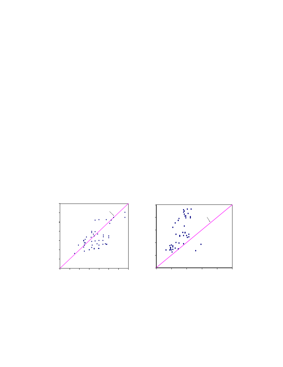
35
2.4.4.
Property Correlations (from Table 2.4)
(i) LL versus Natural Moisture Content
Marine Clay: For 52.9% of the marine clays, the natural moisture content was higher
than the liquid limit indicating the sensitive nature of the clay (Fig. 2.13 (a)). The mean
of the moisture content was 73.6% compared to the mean of the liquid limit of 64.2%.
The coefficient of variations for the moisture content and liquid limits was 30.3% and
34.6%, respectively, indicating similar variability in the two measured parameters.
Deltaic Clay: For 97.9% of the deltaic clays, the natural moisture content was lower than
the liquid limit, opposite of what was observed for the marine clay (Fig. 2.13 (b)). The
mean of the moisture content was 28.9%, compared to the mean of the liquid limit of
53.6%. The coefficient of variations for the moisture content and liquid limits was 32.8%
and 42.4%, respectively. Based on the COV and the standard deviation, the variability in
the liquid limit was higher than the moisture content.
0
20
40
60
80
100
120
140
0
20
40
60
80
100
120
140
Natural water content W
n
(%)
L
iqui
d L
im
it
(
%
)
N = 51
Wn = LL
0
20
40
60
80
100
0
20
40
60
80
100
Natural water content W
n
(%)
Li
qu
id
L
im
it (%
)
Wn = LL
N = 97
(a) Marine clay
(b) Deltaic clay
Fig. 2.13. Liquid Limit versus Natural Water Content for the Soft Clays
(a) Marine Clay and (b) Deltaic Clay.
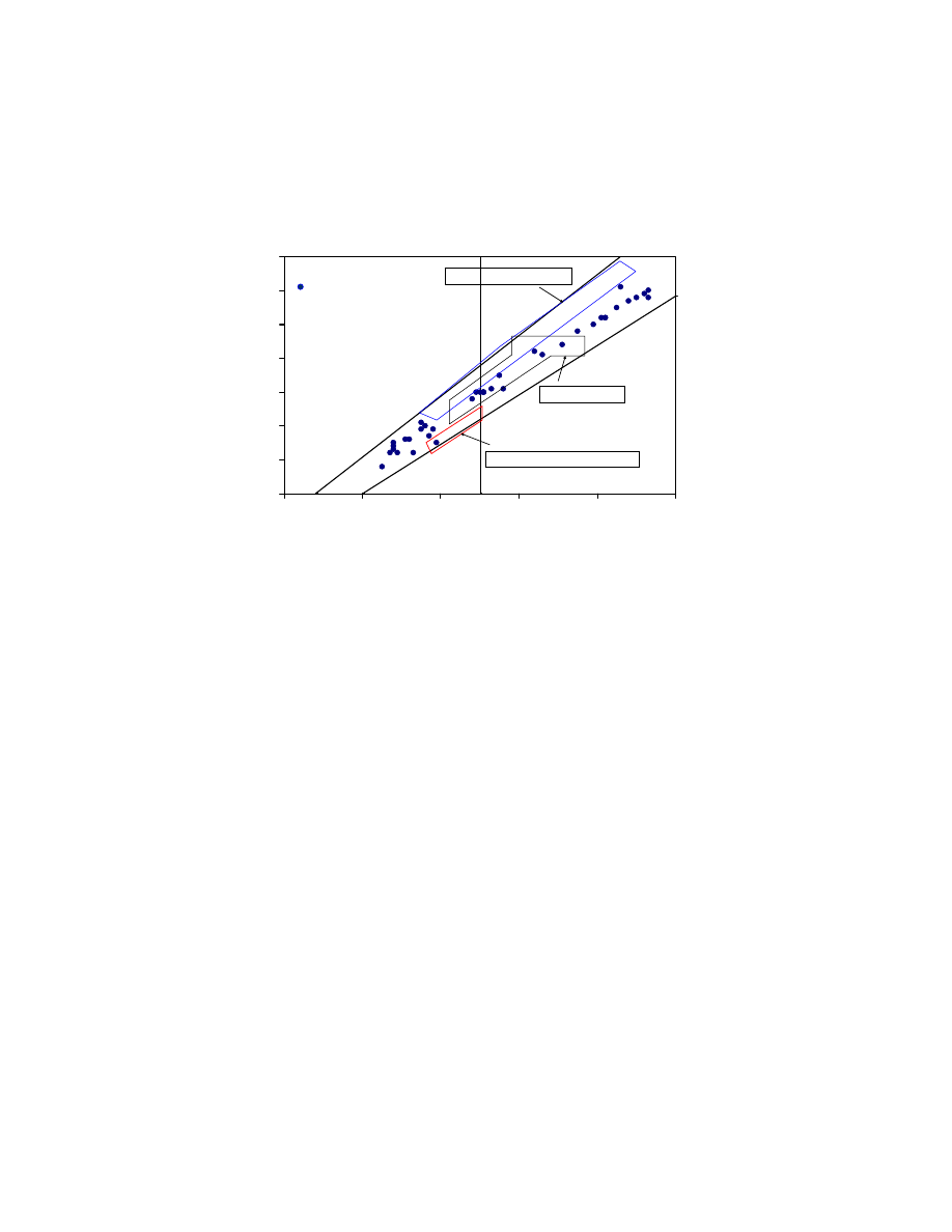
36
(ii) Plasticity Index Chart
0
10
20
30
40
50
60
70
0
20
40
60
80
100
Liquid Limit (%)
P
la
sti
ci
ty
I
n
dex
(%
)
South Korea (Pusan at Gaduko)
Bothkennar (UK)
Bangkok (Sutthisan station)
Houston - Galveston
Fig. 2.14. Plasticity Index chart of Deltaic (42 Data Sets) and Marine Soft Clay Soils.
Marine Clay: The Bangkok and Bothkennar (UK) clays were predominantly CH soils, as
shown in Fig. 2.14. The Bangkok clay showed greater variation in the index properties
than the Bothkennar (UK) clay. The South Korean clay was CL.
Deltaic Clay: Both CH and CL clays are present in the deltaic deposits in the Houston-
Galveston area. Compared to the marine clay, the deltaic clays showed the greatest
variation in the index properties.
(iii) Undrained Shear Strength versus In-situ Stress
Based on the inspection of the undrained shear strength (S
u
) and in-situ vertical
stress (
σ
v
) relationships for the marine clays and deltaic clays (Fig. 2.15 a and b), the
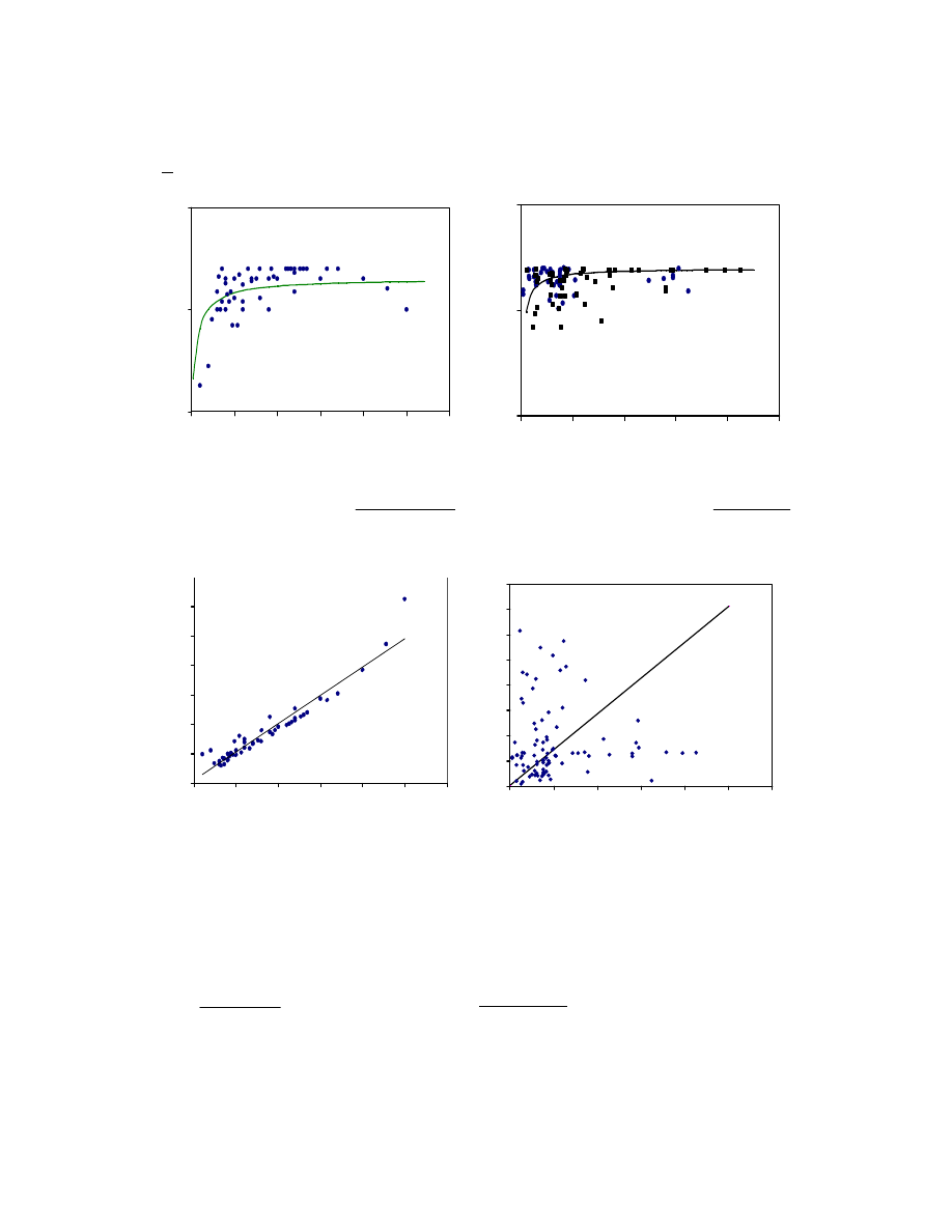
37
following conditions must be satisfied in developing the mathematical relationship. When
σ
v
> 0
1
10
100
0
25
50
75
100
125
150
Vertical pressure
σ
v
(kPa)
U
ndr
ai
ne
d s
he
ar
s
tr
en
gt
h S
u
(
kP
a)
N = 49
1
10
100
0
100
200
300
400
500
Vertical pressure
σ
v
(kPa)
U
n
d
ra
in
ed
s
h
ea
r
st
re
n
gt
h
, S
u
(k
P
a)
N = 95
(a) Marine clay
v
v
u
S
σ
σ
7677
.
0
293
.
2
log
+
=
(b) Deltaic clay
v
v
u
S
σ
σ
7153
.
0
2
log
+
=
y = 0.7677x + 2.293
R
2
= 0.9199
0
20
40
60
80
100
120
140
0
25
50
75
100
125
150
Vertical pressure
σ
v
(kPa)
σ
v
/ lo
g
S
u
N = 49
0
50
100
150
200
250
300
350
400
0
100
200
300
400
500
600
Vertical pressure
σ
v
(kPa)
σ
v
/
lo
g S
u
N = 95
(c) Marine clay
(d) Deltaic clay
Fig. 2.15. Predicted and Measured Relationships for Marine and Deltaic Clays.
0
d
S
log
d
v
u
>
σ
2-22a
0
d
S
log
d
2
v
u
2
<
σ
. 2-22b

38
In this study, the soft clay undrained shear strength was limited to 25 kPa even if the
vertical stress increased indefinitely.
When
∞
⎯→
⎯
v
σ
,
0
d
S
log
d
v
u
=
σ
. 2-23
Also, when
∞
⎯→
⎯
v
σ
,
kPa
25
S
u
⎯→
⎯
.
One mathematical relationship that will satisfy these conditions is the two-parameter
hyperbolic equation, which can be represented as follows
v
B
A
v
u
S
log
σ
σ
+
=
.
2-24
When the vertical overburden stress (
σ
v
) tends to infinity, the undrained shear stress
reaches its theoretical maximum (logS
u
ult
), and it will be related to parameter B as
follows:
logS
u ult
= 1/B with S
u
ult
= 25 kPa.
One way to verify the applicability of Equation 3-4 to the log S
u
-vertical stress (
σ
v
) data
is to rearrange the equation to represent a linear relationship as follows:
σ
v
/ logS
u
= A + B
σ
v
.
2-25
If the data can be represented by a linear relationship (Equation 2-25) within an
acceptable limit (high coefficient of correlation), then it can be stated that the load-
displacement relationship is hyperbolic. Parameters A and B can be obtained from the
linear relationship. Fig. 2-15 (c) and (d) show the typical plot of
σ
v
/ logS
u
versus
σ
v
for
the marine and deltaic clays.
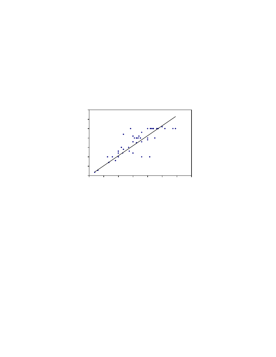
39
Marine Clay: Of the two types of deposits investigated, the hyperbolic relationship
better represented the marine clay. The parameters A
M
and B
M
for the marine clay were
2.293 and 0.7677, respectively, with a coefficient of correlation (R
2
) of 0.9199.
Deltaic Clay: The parameters A
D
and B
D
for the deltaic clay were 2 and 0.7153,
respectively.
(iii) Undrained Shear Strength versus Preconsolidation pressure (
σ
p
)
0
5
10
15
20
25
30
35
0
20
40
60
80
100
120
140
Preconsolidation pressure
σ
p
(kPa)
Undr
ai
ne
d s
he
ar
s
tr
eng
th S
u
(k
P
a)
N = 47
Fig. 2.16. Relationship between Undrained Shear Strength (S
u
) and Preconsolidation
Pressure (
σ
p
).
Marine Clay: Based on over 50 data sets collected from the literature, the relation
between S
u
and
σ
p
was linear, as presented in the literature. The S
u
/
σ
p
ratio was 0.27,
with a coefficient of correlation (R) of 0.82. The S
u
/
σ
p
ratio proposed by Mesri (1988)
was 0.22.

40
2.4.5. Summary and discussion
Based on the literature review and data available in the literature on soft marine
and deltaic clays, properties and correlations were investigated. Houston-Galveston area
soils are deltaic deposits. Based on the review and analyses of the data collected, the
following conclusions can be advanced:
(1) Several analytical methods are available to determine the increase in the in-situ
stresses due to the construction of an embankment. In most cases, 1-D
consolidation theory was used to predict the total and rate of settlement.
(2) Several test methods are available to determine the consolidation properties of soft
clays.
(3) Several mean properties of the marine and deltaic clays have been quantified. The
mean physical (moisture content, void ratio) and geotechnical properties (liquid
limit, plastic limit) of marine clays were higher than those of the deltaic clays. The
mean undrained shear strength of the two deposits was comparable. The natural
moisture content of over 52% in the marine clays was higher than the liquid limit,
but the trend was reversed for the deltaic clays.
(4) Based on the COV, the marine clay showed greater variation in the natural
moisture content (w
n
), undrained shear strength (S
u
), and void ratio (e
o
), compared
to the deltaic clay deposit. Similarly, deltaic clay showed greater variation in
plasticity limit and plasticity index (limited data), compared to the marine clay.
(5) Based on the COV, the deltaic clay properties had higher values than the marine
clay properties, except for the undrained shear strength. It is of interest to note that
the natural moisture content and void ratio had similar values for marine and

41
deltaic deposits. Variation in the properties of the deltaic clays was higher than the
marine clays. Also, the probability distribution functions (pdf) for the various
properties have been determined. The pdf for the marine and deltaic clays were
similar.


43
3. DESIGN AND ANALYSIS OF HIGHWAY EMBANKMENTS
3.1. Highway
Embankments
In the greater Houston area, embankments are used by TxDOT in road
construction. As a coastal city, the Houston-Galveston soil formation is deltaic (O’Neill
and Yoon 1995): an alternation of clay, silty clay (very soft, soft, medium, and stiff), silt,
and sand layers in the top 100 ft, leading to a big scatter in the soil parameters with depth
(Vipulanandan et al. 2007). The soft soil below the ground water is considered to be the
cause of settlement of heavy structures. Hence four embankments on soft soils were
selected for detailed analyses.
Current practice used to estimate the consolidation settlement magnitudes and
settlement rates in TxDOT Projects are as follows:
- subsurface investigations to recover undisturbed samples using Shelby tubes
- incremental load (IL) consolidation test in the laboratory
- estimation of the settlements using 1-D consolidation theory, using the soil
parameters from the IL consolidation tests.
3.1.1. Locations and clay soil types
All four highway embankments were located in the Houston area, with its deltaic
soil formation (Fig. 3.1 and Table 3.1).

44
1
3
4
2
1
3
4
2
Fig. 3.1. Houston Area with the Selected Four Embankments.
45
Table 3.1. Summary In
formation on the Four Selected Embankmen
ts.
Sl
No
Refere
nce
Status
Location
Aver
age
so
ft
cl
ay l
ayer
th
ickness (f
t)
S
u
(psi
)
Emban
kmen
t
Siz
e HxB
(f
tx
ft
)
Instrumentation Settleme
nt
estimation
(in)
1A
Tx
DOT
Pr
oj
ec
t
N
o. 0
508
-02
-10
1
(200
2)
New
IH
10
at
S
H
99
Eastside Borings
99
-1
a & 99
-8
a
20
to
35
2.
85
to
15
.15
12
x 120
N
on
e
3.
19
1B
Tx
DOT
Pr
oj
ec
t
N
o. 0
508
-02
-10
1
(200
2)
New
IH
10
at
S
H
99
Westside B
ori
ng
99
-1a
35
6.
15
to
9.
05
9 to 24
x
12
0
N
on
e
5.
27
to
8.
99
2 TxD
O
T
Proj
ect
N
o. 0
028
-02
-08
1
(200
6)
New
US 9
0
at Oates
Rd
47.5
to 58.
25
-
27.5
to 28 x
22
0 t
o
23
4
No
ne
7.
37
to
9.
42
3 TxD
O
T
Proj
ect
N
o. 0
051
-03
-06
9
(199
3)
Co
m
pleted
in
199
3
SH3
Clear Creek
30
3
to
13
.8
10
.5 x 108
Pr
opo
sed
in
st
rum
ent
at
ion:
dem
ec
poi
nt
s, i
ncl
in
om
et
er,
pi
ezo
m
eter, ten
sio
m
eter
and exte
ns
om
et
er
8.
50
4 TxD
O
T
Proj
ect
N
o. 0
981
-01
-10
4
(200
0)
Co
m
pleted
in
200
0
NA
SA
Rd
1:
fr
om
Anna
pol
is
to Taylor La
ke
65
2
to
14
.5
20
x 60
Pr
opo
sed
in
st
rum
ent
at
ion:
piezom
eter and
extens
om
eter
37
.87

46
3.1.2. Objective and analysis
The objective was to review the approaches used in Texas Department of
Transportation (TxDOT) projects for embankment settlements and rate of settlement
estimation.
3.1.3. Project No 1A (I-10 @ SH99)
At the time of review of the data (August 2006), the project was still not under
construction. The designed embankment height was 12 ft, and the base width (W) was
120 ft. The ratio
W
H was 0.10. Several borings were done on site to collect the
geotechnical information. Two soil samples from one boring (99-1a) were used for the
consolidation tests.
• Field tests
The Texas Cone Penetrometer (TCP) test was performed at several locations, and
the information was used to determine the consistency of the soils. Since TCP tests are
performed at 5-ft intervals, the soil consistency thickness can be determined to an
accuracy of 5 ft. The variation of blow counts in Boring 99-1a up to 55 ft is shown in Fig.
3.2. Based on Boring 99-1a, the soft clay (CH) layer thickness was about 35 ft deep (N
TCP
≤ 20). The water table was at a depth of 6.5 ft.
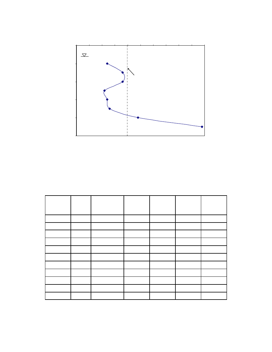
47
Fig. 3.2. Variation of TCP Blow Counts with Depth (Borehole 99-1a.).
Table 3.2. Laboratory Test and Field Tests Results (Borehole 99-1a).
Depth
(ft)
TCP
Soil type
S
u
(psi)
LL (%)
PI (%)
MC (%)
5
CH
7.65
53
36
20
10
12
CH
6.15
58
38
25
15
18
CH
3.75
78
54
29
20
18
82
28
25
11
CH
5.35
71
50
27
30
12
9.05
76
26
35
13
CH
63
39
31
40
24
29
25
45
49
CL
44
26
25
50
11.7
54
21
55
21
0
10
20
30
40
50
0
5
10
15
20
25
30
35
40
45
50
Blow counts/foot
D
epth (
ft
)
Soft Clay
(N
TCP
≤20)
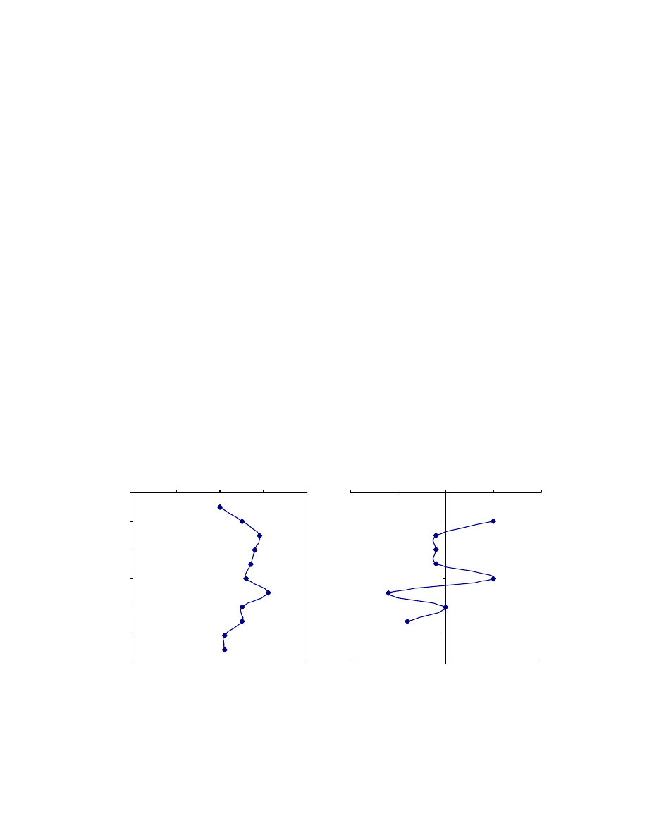
48
• Laboratory tests (Project 1)
Consolidation (IL), moisture content, Atterberg’s limits, and triaxial unconfined
compression tests were performed with the soil samples from Boring 99-1a. The test
results are summarized in Table 3.2 and Table 3.3.
Soil type: Based on the index property tests (Table 3.2) up to 35 ft was CH clay
soil, and below it was CL soil. Also, the moisture content varied from 20% to 30%, as
shown in Fig. 3.3(a). The largest change in moisture content was observed at a depth of
35 ft. The change of moisture content with change in depth (
ΔMC/Δz) versus depth (z) is
shown in Fig. 3.3(b), and the values varied from -1.2 to 1. The highest change was
observed between 35 and 40 ft (representing a change in moisture content of 6%), and
also represented the transition from soft CH to CL clay soil.
The undrained shear strength obtained from the unconfined compression test
varied between 3.75 and 9.05 psi in the top 30 ft of soft CH clay, as shown in Fig. 3.4.
a.) Variation of Moisture Content
b.) Change of Moisture Content
Fig. 3.3. (a) Variation of Moisture Content (MC) with Depth (z) and (b) Change of
Moisture Content with Change in Depth (
ΔMC/Δz).
0
10
20
30
40
50
60
0
10
20
30
40
Moisture Content (%)
D
ep
th
(ft
)
0
10
20
30
40
50
60
-2
-1
0
1
2
∆MC/∆z (%/ft)
D
ep
th
(ft)
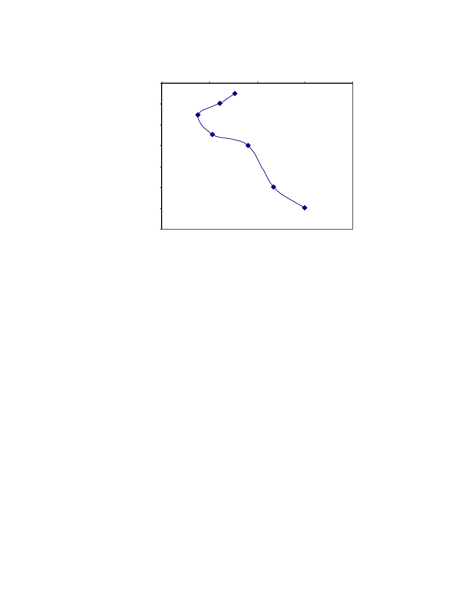
49
Fig. 3.4. Variation of Undrained Shear Strength with Depth (Borehole 99-1a).
• Consolidation properties (Project 1)
The consolidation parameters, summarized in Table 3.3, were obtained from the
standard incremental load consolidation test using samples from Boring 99-1a. Two
consolidation tests were done on samples collected from depths of 5 ft and 25 ft.
Consolidation data obtained from a sample collected at 5 ft depth was used to represent
soil to a depth of 19 ft. The data obtained from a sample collected at the 25 ft depth was
used to represent soil to a depth of 37 ft.
0
10
20
30
40
50
60
70
0
5
10
15
20
S
u
(psi)
De
p
th
(
ft
)
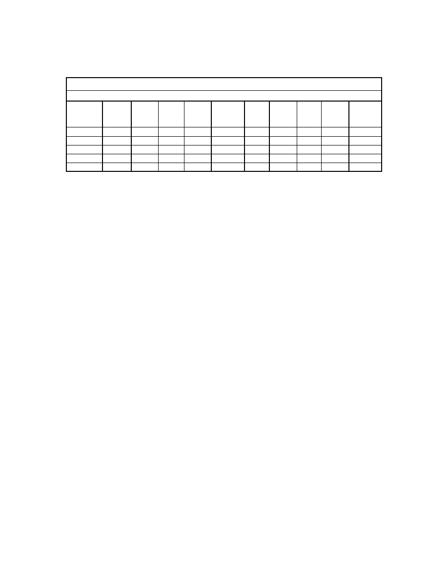
50
Table 3.3. Summary of Consolidation Parameters Used for the Settlement
Estimation.
Depth
(ft)
Layers
height
(ft)
C
c
C
r
e
o
C
v Av
( in
2
/day)
σ
p
(psf)
σ
o
(psf)
OCR
Δσ
(psf)
σ
o
+
Δσ
(psf)
1.50
3
0.174
0.06
0.57
1.06
3800
200
19.0
1672
1872
6.50
7
0.174
0.06
0.57
1.06
3800
607
6.3
1650
2257
14.50
9
0.174
0.06
0.57
1.02
3800
1107
3.4
1613
2720
23.50
9
0.180
0.04
0.70
1.02
5000
1671
3.0
1562
3233
32.50
9
0.180
0.04
0.70
1.02
5000
2234
2.2
1597
3831
Settlement parameters
TxDOT
• Stress Dependency of Consolidation Parameters (C
c
, C
r
)
The stress dependency of the compression and recompression indices was
investigated based on the data available. The samples were loaded to 16 tsf and unloaded
to 0.25 tsf. The slope (-de /dlog
σ
’) was determined for each load increment (Fig. 3.5).
For the sample collected at 5 ft (above the ground water table), the compression
index, along the loading path, varied from 0.010 to 0.083 when the applied load was
increased from 0.25 tsf to 2 tsf and from 0.083 to 0.166 when the applied stress was
increased from 2 tsf to 16 tsf. When unloading, the recompression index (C
r
) varied from
0.048 to 0.058 when the applied load varied from 4 tsf to 0.25 tsf. The C
r
increased with
the reduction of the stress (Fig. 3.5(a)). Hence, C
c
and C
r
are stress dependent parameters.
For the sample collected at 25 ft (below the ground water table), the compression
index, along the loading path, varied from 0.0233 to 0.075 when the applied load was
increased from 0.25 tsf to 2.5 tsf and from 0.075 to 0.179 when the applied stress was
increased from 2.5 tsf to 16 tsf. When unloading, the recompression index (C
r
) varied
from 0.0068 to 0.045 when the applied load varied from 4 tsf to 0.25 tsf. The C
r
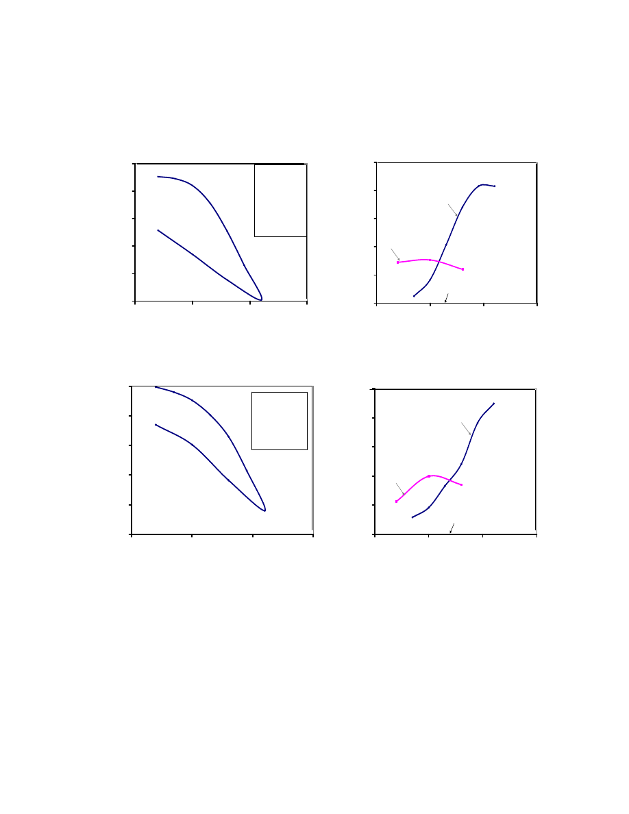
51
decreased with the reduction of the stress after reaching a peak value of 0.08 (Fig. 3.5(a)).
Hence, C
c
and C
r
are stress dependent parameters.
0.38
0.42
0.46
0.50
0.54
0.58
0.1
1.0
10.0
100.0
Vertical effective stress
σ' (tsf)
Void
ratio
e
e
o
= 0.57
σ
p
= 1.9 tsf
C
c
= 0.174
C
r
= 0.058
C
r
/C
c
= 0.333
0.00
0.04
0.08
0.12
0.16
0.20
0.1
1.0
10.0
100.0
Vertical effective stress
σ (tsf)
C
c
&
C
r
C
r
C
c
σ
p
a.) IH10 at SH99 Boring 99-1a at 5ft
0.5
0.54
0.58
0.62
0.66
0.7
0.1
1.0
10.0
100.0
Vertical effective stress
σ' (tsf)
Vo
id
r
at
io
e
e
o
= .694
σ
p
= 2.5 tsf
C
c
= 0.180
C
r
= 0.043
C
r
/C
c
= 0.239
0.00
0.04
0.08
0.12
0.16
0.20
0.1
1.0
10.0
100.0
Vertical effective stress
σ' (tsf)
C
c
&
C
r
C
r
C
c
σ
p
d.) IH10 at SH99 Boring 99-1a at 25ft
Fig. 3.5. e – log
σ’ of the Two Consolidation Tests Performed on TxDOT Project for
1A Embankment Design and Their Respective Compression and Recompression
Index versus log
σ’ Curves (Project 1: I-10 @ SH-99).
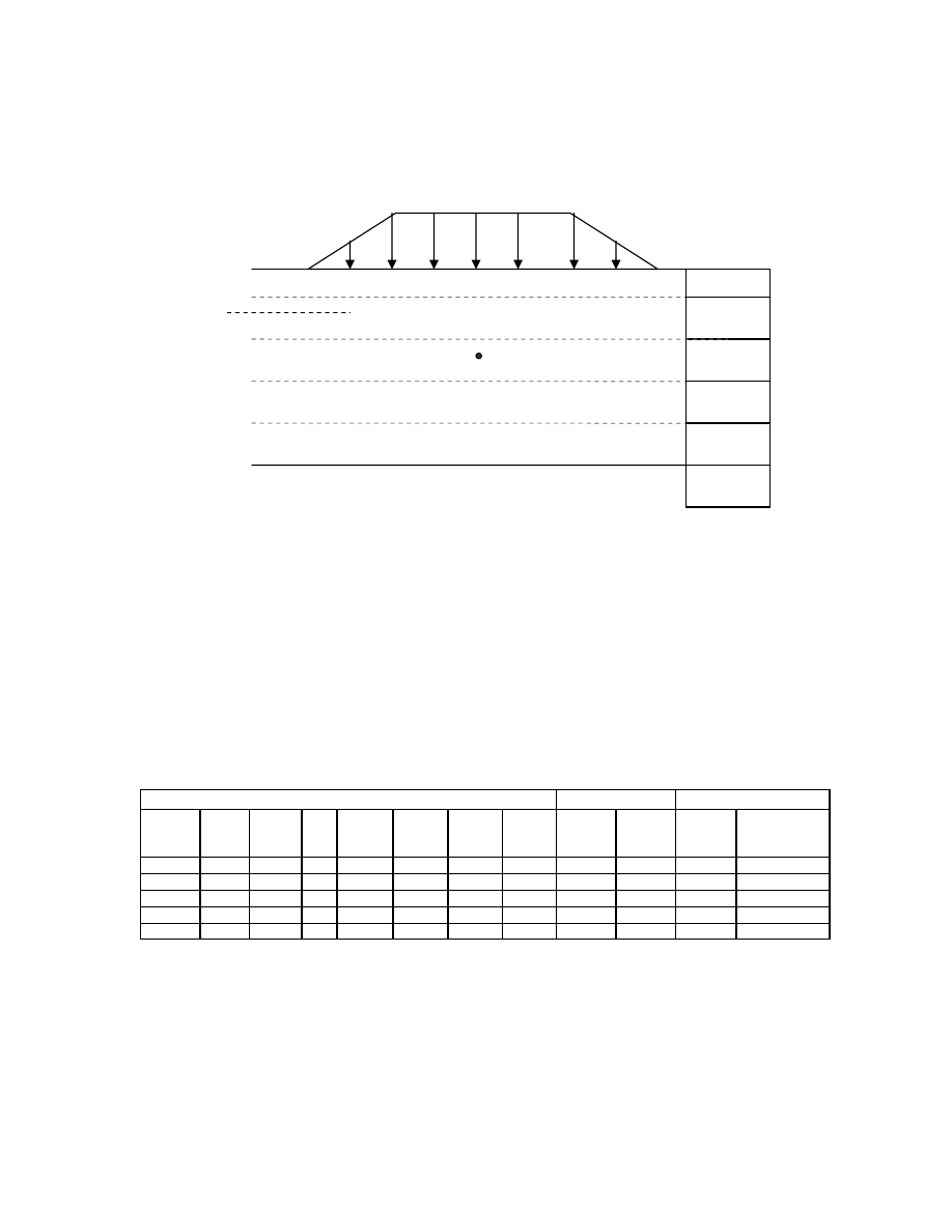
52
• Stress Increase due to embankment loading
Fig. 3.6. Profile of the Soil Layers for Settlement Calculation (Project 1).
The stress increase in the soil mass due to the embankment loading (
Δσ),
(Fig. 3.6), calculated in the TxDOT project, is compared with values obtained using the
Osterberg method and 2:1 method, in Table 3.4 and Fig. 3.7.
Table 3.4. Summary Table of the Stress Increase in the Soil Mass (Project 1).
Depth
(ft)
Depth
(ft)
Layers
height (ft)
σ
p
(psf)
σ
o
(psf)
OCR
Δσ
(psf)
σ
o
+
Δσ
(psf)
Δσ
(psf)
σ
o
+
Δσ
(psf)
Δσ
(psf)
σ
o
+
Δσ (psf)
1.50
1.50
3
3800
200
19.0
1672
1872
1680
1880
1659
1859
6.50
6.50
7
3800
607
6.3
1650
2257
1680
2287
1594
2201
14.50
14.50
9
3800
1107
3.4
1613
2720
1667
2774
1499
2606
23.50
23.50
9
5000
1671
3.0
1562
3233
1631
3302
1405
3076
32.50
32.50
9
5000
2234
2.2
1597
3831
1573
3807
1322
3556
TxDOT
2 : 1 method
Osterberg method
As shown in Fig. 3.7, the stress increase ratio based on TxDOT project approach
to the Osterberg method ranged from 1 to 0.96. But the ratio obtained using the 2:1
method ranged from 1.01 to 1.21. The method used in the TxDOT project, which was
H (ft)
Δσ
W.T. 6.5 ft
CH 3
CH 7
CH 9
CH 9
CH 9
CL
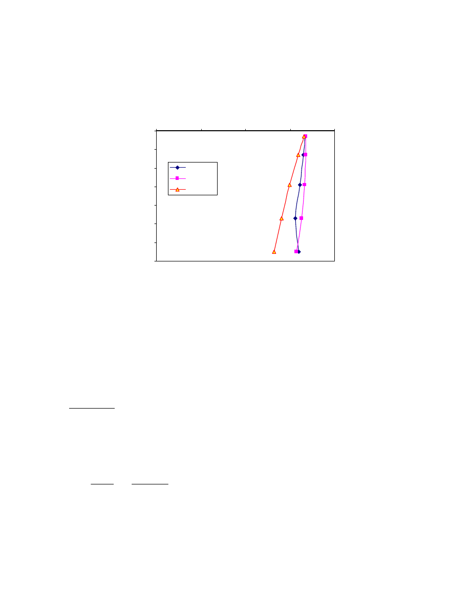
53
specified as Modified Boussinessq method, was very similar to the Osterberg stress
increase calculation method.
0
5
10
15
20
25
30
35
0
500
1000
1500
2000
Stress increase ∆σ (psf)
D
e
p
th
(ft)
TxDOT
Osterberg
2:1
Fig. 3.7. Comparison of Stress Increase Obtained Using the Osterberg, 2:1, and
TxDOT Methods (Project 1).
• Total settlement (Project 1)
Based on the information provided, the settlement estimation by the TxDOT
project approach was 6.10 in. for the total primary settlement.
UH Check: In all the layers, the total stress (
Δσ’ + σ’
o
) was less than the
preconsolidation pressure (
σ
p
). Therefore, the recompression index (C
r
) was the
governing parameter for the total primary settlement S
p
:
⎟
⎟
⎠
⎞
⎜
⎜
⎝
⎛
+
+
=
0
'
'
0
0
p
log
e
1
CrH
S
σ
σ
Δ
σ
.

54
Using Osterberg’s stress increase results (Table 3.4), the following result was obtained:
Layer 1:
ft
1116
.
0
200
1880
log
57
.
0
1
3
x
06
.
0
S
p
=
⎟
⎠
⎞
⎜
⎝
⎛
+
=
Layer
2:
ft
1541
.
0
607
2287
log
57
.
0
1
7
x
06
.
0
S
p
=
⎟
⎠
⎞
⎜
⎝
⎛
+
=
Layer
3:
ft
1372
.
0
1107
2774
log
57
.
0
1
9
x
06
.
0
S
p
=
⎟
⎠
⎞
⎜
⎝
⎛
+
=
Layer
4:
ft
0626
.
0
1671
3302
log
70
.
0
1
9
x
04
.
0
S
p
=
⎟
⎠
⎞
⎜
⎝
⎛
+
=
Layer
5:
ft
0490
.
0
2234
3807
log
70
.
0
1
9
x
04
.
0
S
p
=
⎟
⎠
⎞
⎜
⎝
⎛
+
=
.
Hence the total primary settlement was
Sp = 0.1116 + 0.1541+ 0.1372 + 0.0626 + 0.0490 = 0.5145 ft = 6.17 in.
The difference between the UH and TxDOT project estimations was 0.07 in. It
must be noted that for the consolidation parameters defined in Chapter 4 (C
r1
, C
r2
, and
C
r3
), C
r3
was used in the calculation instead of C
r1
since no other data were available.
• Rate of settlement (Project 1)
TxDOT Project Approach
The TxDOT rate of settlement estimation in the TxDOT project, using C
v
values
in Table 3.3, predicted a settlement of 4.24 in. after 48 months, which represented
69.47% of the total primary settlement (6.10 in.). This result was obtained by considering
the following drainage condition for each layer:
- Layer 1 had two drainage surfaces: top and bottom boundaries
- Layer 2 had two drainage surfaces: top and bottom boundaries

55
- Layer 3 had one drainage surface: top or bottom boundaries
- Layer 4 had one drainage surface: top or bottom boundaries
- Layer 5 had two drainage surfaces: top and bottom boundaries.
The rate of settlement was then calculated for each layer, and for a specific time
(48 months in this case) the total settlement was the sum of the settlements of all layers.
(a) Calculations
48 months = 48 x 30 days
The time factor as defined in Chapter 2 is given by
2
dr
v
v
H
t
c
T
=
.
2-13
The average degree of consolidation is given by the following equation
(Das 2006)
(
)
(
)
[
]
179
.
0
8
.
2
v
5
.
0
v
/
T
4
1
/
T
4
100
%
U
π
π
+
=
. 3-1
Hence if T
v
is determined, the degree of consolidation (U%) can be calculated using
Equation (3-1)
Layer
1;
(
)
(
)
⎯→
⎯
=
=
71
.
4
12
x
5
.
1
30
x
48
06
.
1
T
2
v
U% = 99.67
Layer
2;
(
)
(
)
⎯→
⎯
=
=
865
.
0
12
x
5
.
3
30
x
48
06
.
1
T
2
v
U% = 90.34
Layer
3;
(
)
(
)
⎯→
⎯
=
=
126
.
0
12
x
9
30
x
48
02
.
1
T
2
v
U% = 40.01

56
Layer
4;
(
)
(
)
⎯→
⎯
=
=
126
.
0
12
x
9
30
x
48
02
.
1
T
2
v
U% = 40.01
Layer
5;
(
)
(
)
⎯→
⎯
=
=
504
.
0
12
x
5
.
4
30
x
48
02
.
1
T
2
v
U% = 76.55
Consequently the total settlement S
p48
after 48 months was
S
p48
= (0.9967 x 0.1116) + (0.9034 x 0.1541) + (0.1372 x 0.4001) + (0.0626 x 0.4001) +
(0.0490 x 0.7655)
= 0.3677 ft
= 4.41 in.
The difference of 0.17 in. as compared to the TxDOT result (4.24 in.) could be
due to the approximation of the average degree of consolidation (U%).
One layer consideration
Method 1
Considering two drainages surfaces (top and bottom), the primary settlement
reached after 48 months was calculated using the following procedure:
Weighted average of the coefficient of consolidation
(
) (
)
day
/
in
031
.
1
37
x
12
02
.
1
x
27
x
12
06
.
1
x
10
x
12
H
H
C
C
2
i
i
vi
v
=
+
=
∑
∑
=
(
)
(
)
58
.
19
%
U
0301
.
0
12
x
5
.
18
30
x
48
031
.
1
H
t
c
T
2
2
dr
v
v
=
⎯→
⎯
=
=
=
.
S
p48
= 0.1958 x 6.17 = 1.21 in.
Based on this approach, the settlement after 48 months will be 1.21 in.,
representing 20% of the total primary settlement.

57
Method 2
Considering two drainages surfaces (top and bottom), the necessary time to reach
69.47% of primary settlement was calculated using the following procedure.
Weighted average of the coefficient of consolidation
(
) (
)
day
/
in
031
.
1
37
x
12
02
.
1
x
27
x
12
06
.
1
x
10
x
12
H
H
C
C
2
i
i
vi
v
=
+
=
=
∑
∑
(
)(
)
(
)
[
]
357
.
0
6
.
5
2
v
100
/
%
U
1
100
/
%
U
4
/
T
−
=
π
3-2
With U% = 69.47%, Tv = 0.398
(
)
day
025
,
19
031
.
1
12
x
5
.
18
398
.
0
C
H
T
t
2
v
2
dr
v
=
=
=
= 634 months = 53 years.
Hence the time taken for consolidation of 69.47% was 634 months, which was
more than 13 times the 48 months estimated by the TxDOT project approach and the
results are compared in Fig. 3.8.
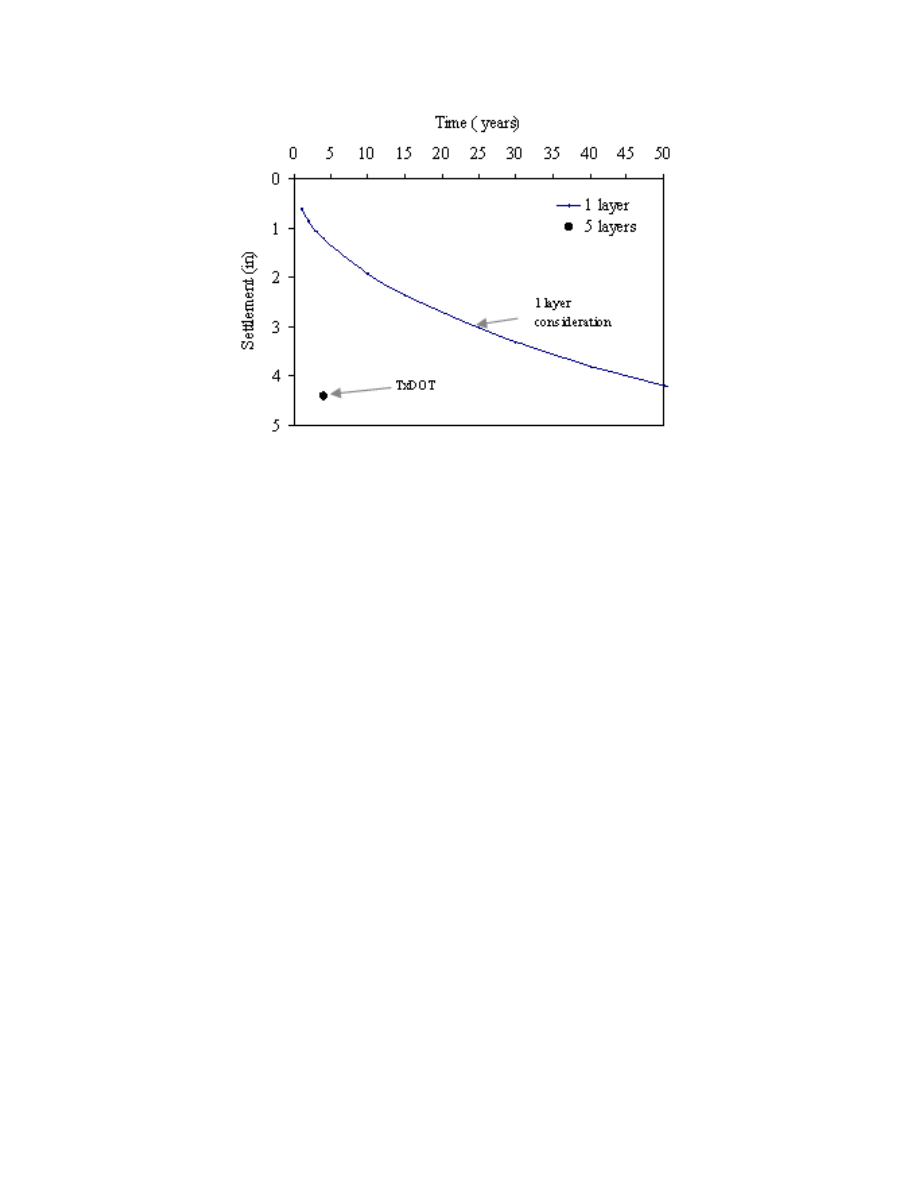
58
Fig. 3.8. Comparison of the Rate of Settlement by Various Methods of Estimation.
Comments on the settlement prediction (Project 1)
- All the predictions are based on two consolidation tests. These two tests are
representing 37 ft of soil. The number of tests is not representative of the
variability in deltaic soil deposits. At least one consolidation test should be
done every 6 ft of depth to better estimate the consolidation properties.
- The method used to estimate the stress increase was similar to the Osterberg
method.
- Since the applied load on the soft soil was less than the preconsolidation
pressure, the slope of the unloading section of the e –log
σ’ curve (C
r
) was
used for estimating the settlement. It must be noted that the recompression
index varied with the applied stress.
- The method used in the TxDOT project had layers of soft soils to estimate the
time of settlement. This approach underestimated the time of settlement and is

59
not correct (based on theory) because of the assumed drainage condition for
each layer.
3.1.4.
Project No 2 (US 90 @ Oates Road)
At the time of review of the data (August 2006), the project was still not under
construction. The designed embankment height (H) was 22.7 ft and the base width (W)
was 220 ft. The ratio W
H
was 0.125. Four borings were taken up to a depth of 80 ft to
collect the geotechnical information. Four samples were used for the consolidation tests.
• Field tests (Project 2)
The Texas Cone Penetrometer (TCP) test was performed at several locations to
determine the soil layers’ strength and to identify the soft soil (Tables 3.5 through 3.8).
TCP tests were performed at 5-ft intervals; consequently, the soil consistency thickness
was determined to an accuracy of 5 ft. The variations of blow counts in these borings
(O-1, O-4, O-5 and O-6) are shown in Fig. 3.9. Based on the TCP blow count, the soft
clay layer thickness was about 30 ft deep (TCP ≤ 20). The water table was located at a
depth of 15 ft (Fig. 3.9).
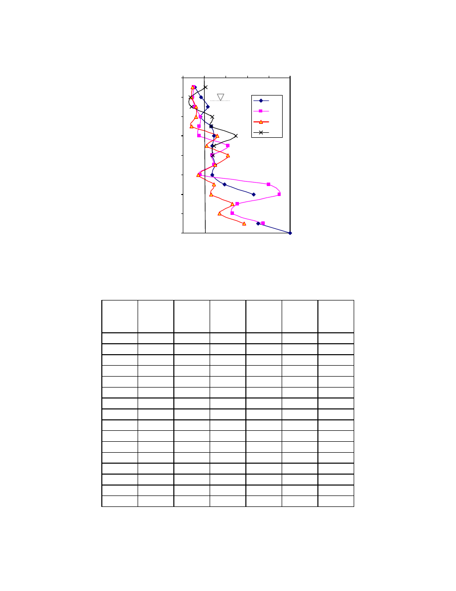
60
Fig. 3.9. Variation of TCP Blow Counts with Depth (Project 2).
Table 3.5. Laboratory and Field Tests Results (Boring O-1) (Project 2).
Depth
(ft)
TCP
Type
S
u
(psi)
LL (%)
PI (%)
MC (%)
5
11
CH
12.30
60
42
18
10
17
CL
6.15
21
15
23
CL
3.75
32
22
20
16
CL
14.88
23
25
26
CL
18.95
45
31
17
30
29
CH
10.90
67
42
28
35
27
CH
12.30
26
40
27
CH
17.05
27
45
30
CH
9.75
35
50
27
CH
83
34
55
39
CL
11.00
33
21
60
66
CL
16
65
CL
34.10
16
70
SAND
75
70
SAND
80
100
0
10
20
30
40
50
60
70
80
0
20
40
60
80
100
Blow counts / foot
D
ep
th (ft)
O-1
O-4
O-5
O-6

61
Table 3.6. Laboratory and Field Tests Results (Boring O-4) (Project 2).
Depth
(ft)
TCP
Type
S
u
(psi)
LL (%)
PI (%)
MC (%)
5
10
CH
6.90
69
51
20
10
9
CL
2.90
15
11
CL
27
19
20
16
CL
8.35
19
25
15
CL
8.20
27
17
30
15
CH
19.85
17
35
42
CH
14.75
25
40
27
CH
10.65
70
47
29
45
29
CH
27
50
16
CL
8.90
33
19
55
80
SC
21
60
90
CL
27.95
45
30
18
65
51
CL
22.90
38
17
70
46
CL
22
19
75
75
CL
19
22
80
62
Table 3.7. Laboratory and Field Tests Results (Boring O-5) (Project 2).
Depth
(ft)
TCP
Type
S
u
(psi)
LL (%)
PI (%)
MC (%)
0
CL
5
9
CH
7.00
22
10
8
CH
4.10
26
15
12
CL
5.63
45
23
20
12
CL
6.65
19
25
8
CL
9.25
23
19
30
32
CL
14
35
22
CL
11.73
22
40
42
CH
25.70
18
45
30
CH
23.33
75
49
26
50
14
CH
81
31
55
29
CH
14.45
80
31
60
26
CH
18.85
81
54
33
65
46
SC
22
7
21
70
34
SC
18
75
57
CH
60
25
80
Table 3.8. Laboratory and Field Tests Results (Boring O-6) (Project 2).
Depth
(ft)
TCP
Type
S
u
(psi)
LL (%)
PI (%)
MC (%)
5
21
CH
7.50
64
23
10
7
CH
2.85
28
15
8
CH
4.65
52
29
20
27
CL
13.30
39
24
24
25
26
CL
12.65
25
28
30
39
CL
40
26
21
35
29
CL
11.00
37
17
40
28
CH
13.30
64
23

63
• Laboratory tests
Incremental load consolidation, moisture content, Atterberg’s limits, and triaxial
unconfined compression tests were performed with the samples from the four borings.
The results are summarized in (Tables 3.5 through 3.9).
Soil type: Based on the index property tests, the top 5 to 25 ft was mainly CL clay
over a 25 ft-deep layer of CH clay. Also, the moisture content variation shown in
Fig. 3.10(a) fluctuated between 15 and 35%. The largest change in moisture content was
observed at a depth of 55 ft in Boring O-1. The change in moisture content with change
in depth (
ΔMC/Δz) versus depth (z), (Fig. 3.10(b)) values ranged from -2.7 to 2.1, with
the highest change between 50 and 55 ft in Boring O-1, representing a change in moisture
content of -13%, and was the transition from CH to CL clay soil.
The undrained shear strength obtained from the unconfined compression test
varied between 2.90 and 25.70 psi in the top 50 ft of clay soil, as shown in Fig. 3.11.
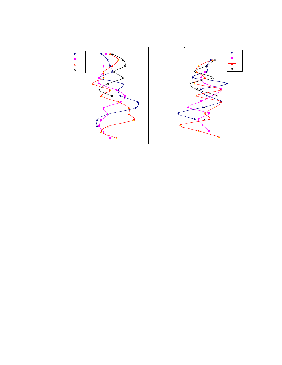
64
a.) Variation of Moisture Content
b.) Change of Moisture Content
Fig. 3.10. (a) Variation of Moisture Content (MC) with Depth (z) and (b) Change of
Moisture Content with Change in Depth (
ΔMC/Δz) (Project 2).
0
10
20
30
40
50
60
70
80
0
10
20
30
40
Moisture Content (%)
D
ept
h (
ft
)
O-1
O-4
O-5
O-6
0
10
20
30
40
50
60
70
80
-4
-2
0
2
4
ΔMC/ΔZ (%/ft)
D
ept
h (
ft)
O-1
O-4
O-5
O-6
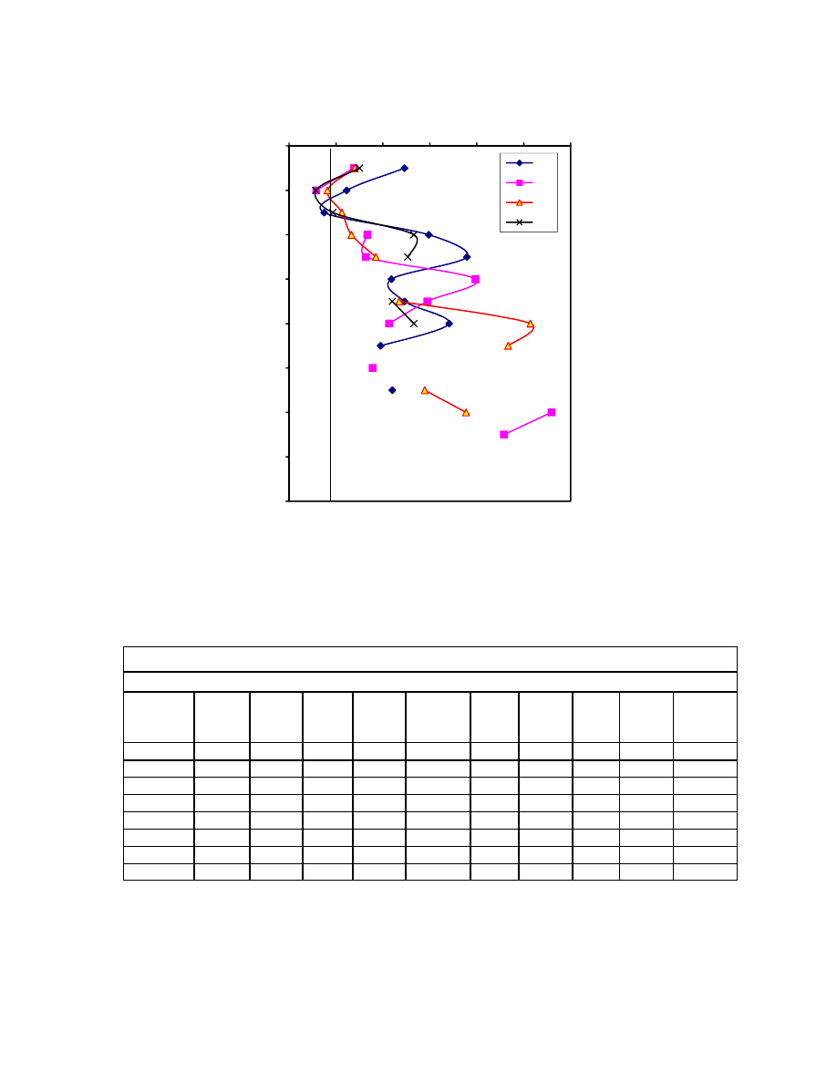
65
0
10
20
30
40
50
60
70
80
0
5
10
15
20
25
30
D
epth (ft)
S
u
(psi)
O-1
O-4
O-5
O-6
Fig. 3.11. Variation of Undrained Shear Strength with Depth (from the Four
Borings) (Project 2).
Table 3.9. Summary Table of Consolidation Parameters Used for the Settlement
Estimation (Project 2).
Depth
(ft)
Layers
height
(ft)
C
c
C
r
e
o
C
v Av
( in
2
/day)
σ
p
(psf)
σ
o
(psf)
OCR
Δσ
(psf)
σ
o
+
Δσ
(psf)
2.5
5.0
0.279
0.021
0.75
0.5
4600
313
14.7
3540
3853
7.5
5.0
0.202
0.021
0.68
1.6
3400
938
3.6
3540
4478
12.5
5.0
0.202
0.021
0.68
1.6
3400
1407
2.4
3538
4945
18.8
7.5
0.138
0.008
0.69
1.0
4400
1798
2.4
3533
5331
26.3
7.5
0.138
0.008
0.69
1.0
4400
2267
1.9
3521
5788
33.5
7.0
0.155
0.036
0.56
0.7
6600
2721
2.4
3502
6223
40.5
7.0
0.155
0.036
0.56
0.7
6600
3159
2.1
3476
6635
47.5
7.0
0.155
0.036
0.56
0.7
6600
3598
1.8
3442
7040
Settlement parameters
TxDOT
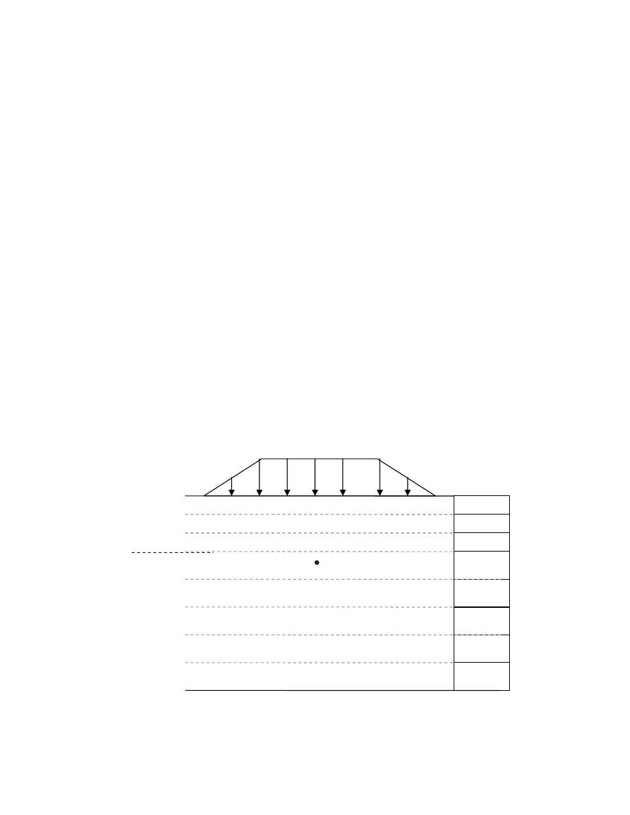
66
• Consolidation properties (Project 2)
The consolidation parameters, summarized in Table 3.9, were determined from
the standard incremental load consolidation test using the samples from the borings. A
total of four IL consolidation tests were performed.
• Stress Dependency Phenomena (C
c
, C
r
)
The e – log
σ’ of the four consolidation tests were not available to study the stress
dependency of compression (C
c
) and recompression (C
r
) indices.
• Stress Increase due to embankment loading (Project 2)
The stress increase in the soil mass due to the embankment loading (
Δσ),
calculated by TxDOT project approach, (Fig. 3.12), is compared with values obtained
using the Osterberg and 2:1 methods, as shown in Table 3.10 and Fig. 3.13.
Fig. 3.12. Profile of the Soil Layers for Settlement Calculation (Project 2).
H (ft)
W.T. 15 ft
Δσ
CH 5
CH 7.5
CH 7.5
CH 7.5
CL 7
CL 7
CH 5
CH 5
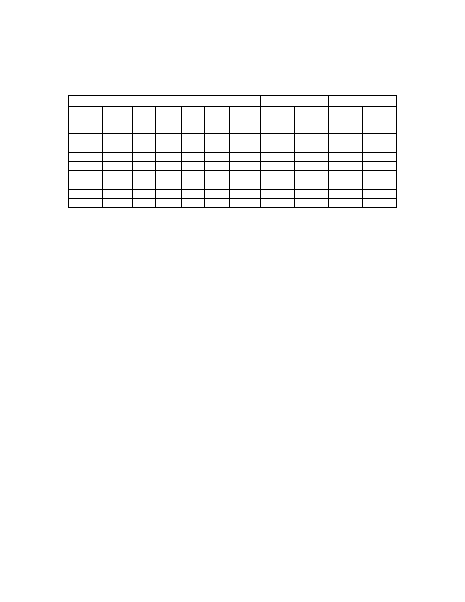
67
Table 3.10. Summary Table of the Stress Increase in the Soil Mass.
Depth
(ft)
Layers
height (ft)
σ
p
(psf)
σ
o
(psf)
OCR
Δσ
(psf)
σ
o
+
Δσ
(psf)
Δσ
(psf)
σ
o
+
Δσ
(psf)
Δσ
(psf)
σ
o
+
Δσ
(psf)
2.5
5.0
4600
313
14.7
3540
3853
3540
3853
3500
3813
7.5
5.0
3400
938
3.6
3540
4478
3538
4476
3423
4361
12.5
5.0
3400
1407
2.4
3538
4945
3526
4933
3350
4757
18.8
7.5
4400
1798
2.4
3533
5331
3493
5291
3262
5060
26.3
7.5
4400
2267
1.9
3521
5788
3429
5696
3163
5430
33.5
7.0
6600
2721
2.4
3502
6223
3347
6068
3072
5793
40.5
7.0
6600
3159
2.1
3476
6635
3256
6415
2990
6149
47.5
7.0
6600
3598
1.8
3442
7040
3162
6760
2911
6509
TxDOT
Osterberg method
2 to 1 method
As observed in Fig. 3.13, the TxDOT project approach stress increase values were
higher than the Osterberg and 2:1 methods. The ratio of the TxDOT project approach
values to the Osterberg’s values ranged from 1 to 1.09, and the ratio obtained with the 2:1
method ranged from 1.01 to 1.18. The TxDOT project approach, which was specified as
the Modified Boussinessq method, was closer to the Osterberg stress increase calculation
method.
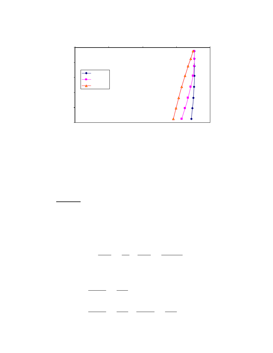
68
0
10
20
30
40
50
0
1000
2000
3000
4000
Stress increase (psf)
D
ep
th (ft)
TxDOT
Osterberg
2:1
Fig. 3.13. Comparison of Stress Increase Obtained Using Osterberg and 2:1 and
TxDOT Methods.
• Total settlement (Project 2)
Based on the TxDOT project approach settlement estimation was 7.13 in. for the
total primary settlement.
UH Check: In five layers out of eight, the total effective stress (
Δσ’ + σ’
o
) was
higher than the preconsolidation pressure (Table 3.10). Therefore, the compression (C
c
)
and recompression index (C
r
) were both the governing parameters of the total primary
settlement S
p,
⎟
⎟
⎠
⎞
⎜
⎜
⎝
⎛
+
+
+
⎟
⎟
⎠
⎞
⎜
⎜
⎝
⎛
+
=
p
'
'
0
0
c
'
0
p
0
r
p
log
e
1
H
C
log
e
1
H
C
S
σ
σ
Δ
σ
σ
σ
.
Using Osterberg’s stress increase results (Table 3.10), we obtained the following results:
Layer 1:
ft
0654
.
0
313
3853
log
75
.
0
1
5
x
021
.
0
S
p
=
⎟
⎠
⎞
⎜
⎝
⎛
+
=
Layer
2:
ft
1067
.
0
3400
4476
log
68
.
0
1
5
x
202
.
0
938
3400
log
68
.
0
1
5
x
021
.
0
S
p
=
⎟
⎠
⎞
⎜
⎝
⎛
+
+
⎟
⎠
⎞
⎜
⎝
⎛
+
=

69
Layer
3:
ft
1211
.
0
3400
4933
log
68
.
0
1
5
x
202
.
0
1407
3400
log
68
.
0
1
5
x
021
.
0
S
p
=
⎟
⎠
⎞
⎜
⎝
⎛
+
+
⎟
⎠
⎞
⎜
⎝
⎛
+
=
Layer
4:
ft
0628
.
0
4400
5291
log
69
.
0
1
5
.
7
x
138
.
0
1798
4400
log
69
.
0
1
5
.
7
x
008
.
0
S
p
=
⎟
⎠
⎞
⎜
⎝
⎛
+
+
⎟
⎠
⎞
⎜
⎝
⎛
+
=
Layer 5:
ft
0789
.
0
4400
5696
log
69
.
0
1
5
.
7
x
138
.
0
2267
4400
log
69
.
0
1
5
.
7
x
008
.
0
S
p
=
⎟
⎠
⎞
⎜
⎝
⎛
+
+
⎟
⎠
⎞
⎜
⎝
⎛
+
=
Layer 6:
ft
0563
.
0
2721
6068
log
56
.
0
1
7
x
036
.
0
S
p
=
⎟
⎠
⎞
⎜
⎝
⎛
+
=
Layer 7:
ft
0497
.
0
3159
6415
log
56
.
0
1
7
x
036
.
0
S
p
=
⎟
⎠
⎞
⎜
⎝
⎛
+
=
Layer
8:
ft
x
x
S
p
0498
.
0
6600
6760
log
56
.
0
1
7
155
.
0
3598
6600
log
56
.
0
1
7
036
.
0
=
⎟
⎠
⎞
⎜
⎝
⎛
+
+
⎟
⎠
⎞
⎜
⎝
⎛
+
=
.
Hence the total primary settlement was
Sp = 0.0654 + 0.1067 + 0.1211 + 0.0628 + 0.0789 + 0.0563 + 0.0497 + 0.0498
= 0.5907 ft = 7.09 in.
The difference between the UH and TxDOT project approach estimations was
0.04 in. It must be noted that since the e – log
σ’ of the consolidation tests were not
available, the types of recompression indices (C
r1
, C
r2
, C
r3
) (Refer Section 4.6.1) used
were not known.
• Rate of settlement (Project 2)
TxDOT Project Approach
TxDOT project approach rate of settlement estimation, using the C
v
values in
Table 3.9, predicted a settlement of 6.63 in. after 120 months which represented over

70
90% of the total primary settlement (7.13 in.). This result was obtained by considering
two drainage surfaces (top and bottom) for each layer.
The rate of settlement was then calculated for each layer, and for a specific time
(120 months in this case) the total settlement was the sum of the settlements of all layers.
(a) Calculation
120 months = 120 x 30 = 3600 days
2
dr
v
v
H
t
c
T
=
2-13
(
)
(
)
[
]
179
.
0
8
.
2
v
5
.
0
v
/
T
4
1
/
T
4
100
%
U
π
π
+
=
3-1
Layer
1
(
)
(
)
⎯→
⎯
=
=
000
.
2
12
x
5
.
2
3600
5
.
0
T
2
v
U% = 98.64
Layer
2
(
)
(
)
⎯→
⎯
=
=
400
.
6
12
x
5
.
2
3600
6
.
1
T
2
v
U% = 99.70
Layer
3
(
)
(
)
⎯→
⎯
=
=
400
.
6
12
x
5
.
2
3600
6
.
1
T
2
v
U% = 99.70
Layer
4
(
)
(
)
⎯→
⎯
=
=
778
.
1
12
x
75
.
3
3600
0
.
1
T
2
v
U% = 98.19
Layer
5
(
)
(
)
⎯→
⎯
=
=
778
.
1
12
x
75
.
3
3600
0
.
1
T
2
v
U% = 98.19
Layer
6
(
)
(
)
⎯→
⎯
=
=
429
.
1
12
x
5
.
3
3600
7
.
0
T
2
v
U% = 96.90
Layer
7
(
)
(
)
⎯→
⎯
=
=
429
.
1
12
x
5
.
3
3600
7
.
0
T
2
v
U% = 96.90

71
Layer
8
(
)
(
)
⎯→
⎯
=
=
429
.
1
12
x
5
.
3
3600
7
.
0
T
2
v
U% = 96.90.
Consequently the total settlement S
p120
after 120 months was
S
p120
= (0.9864 x 0.0654) + (0.997 x 0.1067) + (0.997 x 0.1211) + (0.9819 x
0.0628) + (0.9819 x 0.0789) + (0.969 x 0.0563) + (0.969 x 0.0497) + (0.969
x 0.0498) = 0.5817 ft = 6.98 in.
There is a difference of 0.35 in. with the TxDOT result of 6.63 in., which could be
partly due to the noted difference in the stress increase and to the approximation of the
average degree of consolidation U%.
One layer consideration
Method 1
Considering two drainage surfaces (top and bottom), the settlement primary
settlement reached after 120 months can be calculated using the following procedure:
Weighted average of the coefficient of consolidation
(
) (
) (
) (
)
day
/
in
943
.
0
5
.
51
7
.
0
x
5
.
21
1
x
15
6
.
1
x
10
5
.
0
x
5
H
H
C
C
2
i
i
vi
v
=
+
+
+
=
=
∑
∑
(
)
(
)
28
.
21
%
U
0355
.
0
12
x
75
.
25
3600
953
.
0
H
t
c
T
2
2
dr
v
v
=
⎯→
⎯
=
=
=
S
p120
= 0.2128 x 7.09 = 1.51 in.
Based on this approach, the settlement after 120 months will be 1.51 in.,
representing about 21% of the total primary settlement.

72
Method 2
Considering two drainage surfaces (top and bottom), the necessary time to reach
90% of primary settlement can be calculated using the following procedure:
Weighted average of the coefficient of consolidation
day
/
in
943
.
0
C
2
v
=
(
)(
)
(
)
[
]
357
.
0
6
.
5
2
v
100
/
%
U
1
100
/
%
U
4
/
T
−
=
π
With U% = 90 %, T
v
= 0.848
(
)
day
85862
943
.
0
12
x
75
.
25
848
.
0
C
H
T
t
2
v
2
dr
v
=
=
=
= 2862 months = 238 years.
This result of 2,862 months was about 24 times more than the TxDOT prediction
of 120 months to reach 90% of the primary settlement (Fig. 3.14).
Comment on the settlement prediction (Project 2)
- All the predictions were based on four consolidation tests. These four tests are
representing 51 ft of soil. The number of tests is not representative of the
variability in deltaic soil deposits. At least one consolidation test should be
done every 6 ft of depth to better estimate the consolidation properties.
- The method used to estimate the stress increase was closer to the Osterberg
method. The soft clay soil was overconsolidated and in five layers out of eight
the total effective stress was higher than the preconsolidation pressure.
Therefore, both the compression and recompression indices are governing
parameters of the total primary settlement. The e –log
σ’ curves of the four
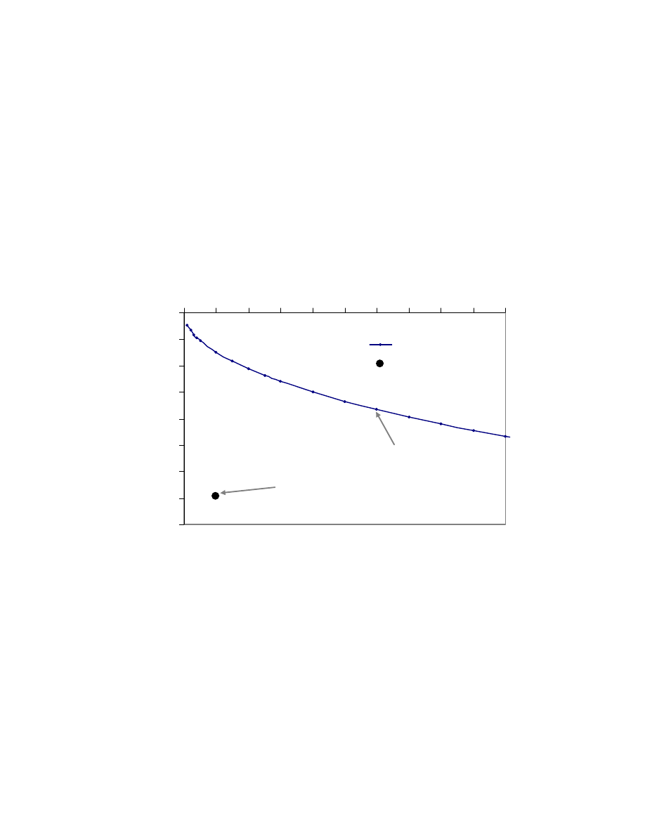
73
consolidation tests were not available. Consequently, the type of the three
recompression indexes used was not known.
- The TxDOT project approach used layers of soft soils to estimate the time of
settlement. This approach underestimated the time of settlement and is not
correct because of the assumed drainage condition for each layer.
0
1
2
3
4
5
6
7
8
0
10
20 30
40 50 60
70 80
90 100
Time ( years)
S
ettle
m
en
t (
in
)
1 layer
8 layers
TxDOT
1 layer
consideration
Fig. 3.14. Effect of Layering on the Rate of Settlement (Project 2).

74
3.1.5. Project No 3 (SH3 @ Clear Creek)
At the time of review of the data (2007), the highway embankment had been in
service for 14 years. The designed embankment height varied from 7.81 to 8.92 ft, and
the base width (W) was 108 ft (Fig. 3.15). The ratio W
H
varied then from 0.07 to 0.08.
About 20 borings were taken on site to collect the geotechnical information from 1965
through 1991 for construction, widening, and modification of the road as follows:
- Through September and October 1965, seven borings (M-1, M-2, M-3, R-1,
R-2, M-12, and R-13) were completed to a 100 ft depth to widen the roadway
and to construct the bridges over Clear Creek and Clear Creek Relief. The
construction work was completed in 1971.
- During February, March, and September of 1984, seven new borings (CCB-1,
CCB-2, CCB-3, CCR-1, CCR-2, CCR-3 and CCR-4) were completed to a
60 ft depth to widen and elevate the North Bridge (NB) roadway, to remove
and replace the NB bridges over Clear Creek and Clear Creek Relief, and to
construct the retaining walls at NB roadway and bridge approaches.
- One boring (CCR-5) was completed to a 75 ft depth in November 1991 for the
removal and replacement of the South Bridge (SB) and construction of
retaining walls at SB Clear Creek Relief bridge approaches. The construction
work was completed in December 1993 (Fig. 3.16).
- Finally, in January 2007, five borings (B1, B2, B3, B4 and B5) were drilled to
a depth of 20 to 30 ft by the University of Houston to assess the embankment
settlement and the retaining wall movement.
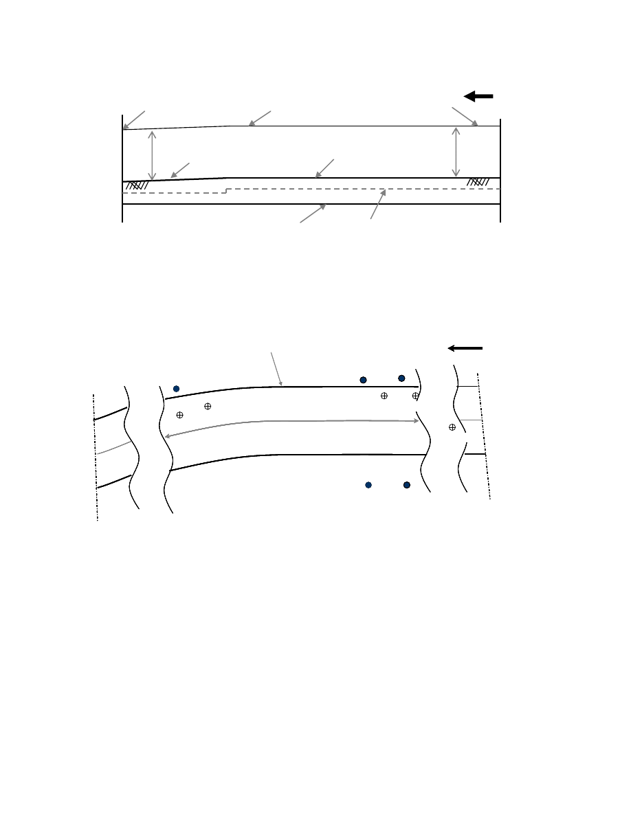
75
Sta. 18 + 60.93
Bridge start
N
Sta. 10+ 12.55
Bridge end
RETAINING WALL No. 2E
Finish grade. Elev. 9.00’
Finish grade. Elev. 8.50’
Elev. 16.31’
Top of the wall.
Elev. 17.92’
Project station
Wall
bottom.
Elev.7.50’
8.
92
’
7.
81
’
Fig. 3.15. Profile of the Retaining Wall No. 2E, Not to Scale (Project 3 Drawing 22).
N
840 ft
N
Retaining wall No. 2E
B1
B2
B4
B3
Clea
r c
reek
Clear c
reek re
lief
840 ft
B5
CCR-2
CCR-4
CCR-3
CCB-1
CCB-2
N
840 ft
N
Retaining wall No. 2E
B1
B2
B4
B3
Clea
r c
reek
Clear c
reek re
lief
840 ft
B5
CCR-2
CCR-4
CCR-3
CCB-1
CCB-2
Fig. 3.16. Location of the Borings Used in the Field (Drawings 13 and 14).
• Field tests (Project 3)
The Texas Cone Penetrometer (TCP) test was performed at 15 locations, and the
information was used to determine the consistency of the soil. Only the Borings CCB-1,
CCB-2, CCR-2, CCR-3, and CCR-4 (Fig. 3.16) data were used for the design of the
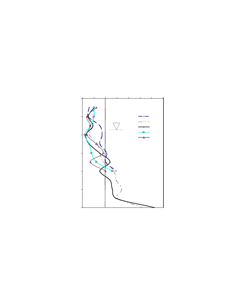
76
embankment. Since the TCP tests are performed at 5-ft intervals (Table 3-11), the soil
consistency thickness can be determined to an accuracy of 5 ft. The variation of blow
counts in the four borings up 40 and 60 ft is shown in Fig. 3.17. Based on the borings, the
soft soil layer thickness was about 45 ft deep (N
TCP
≤ 20). In 2007, the average water
table was at 6.5 ft below the ground and was fluctuating based on the weather.
Fig. 3.17. Variation of TCP Blow Counts with Depth (Project 3).
0
10
20
30
40
50
60
0
10
20
30
40
50
60
70
Blow counts / foot
D
ep
th
(f
t)
CCB-2
CCB-1
CCR-2
CCR-4
CCR-3
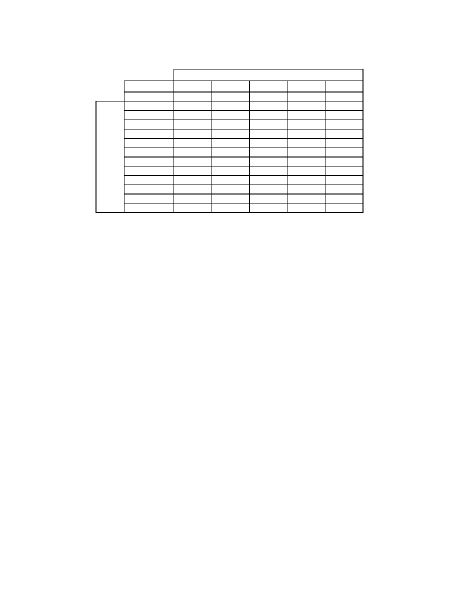
77
Table 3.11. Field Test Results (Borings CCB-2, CCB-1, CCR-2, CCR-4 and CCR-3).
Elevation (ft)
12.3
12.2
12.7
11.9
11.8
Borings
CCB-2
CCB-1
CCR-2
CCR-4
CCR-3
5
6
10
10
10
12
10
5
9
5
10
4
15
15
9
9
7
7
20
17
6
3
2
4
25
15
13
6
6
12
30
21
15
15
8
18
35
20
18
24
12
7
40
29
27
15
26
20
45
29
24
50
34
26
55
30
29
60
52
62
TCP blow count
Bor
ing de
pt
h
(ft
)
• Laboratory tests (Project 3)
The Consolidation (IL) tests were performed on three samples from Boring
CCR-3 in 1984. The moisture content, Atterberg limits, and triaxial unconfined
compression tests were performed with the soil samples from five borings.
Soil type: Based on the index property tests (Table 3.12), the top 5 to 25 ft was
CH clay soil and below it was CL soil. Also, the moisture content varied between 18%
and 44%, as shown in Fig. 3.18(a). The largest change in moisture content was observed
at a depth of 25 ft. The change of moisture content per unit depth (
ΔMC/Δz) versus
depth (z) is shown in Fig. 3.18(b), and the values varied from -11.5 to 6%/ft. The highest
change was observed between 25 and 30 ft in boring CCR-4 (representing a total change
in moisture content of 23%) and was in the very soft (TCP < 8) CH to CL clay soils.
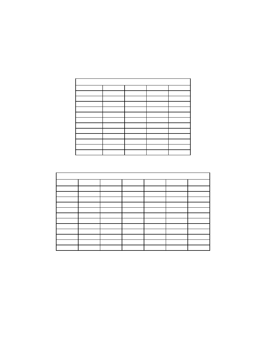
78
The undrained shear strength obtained from the unconfined compression test
varied between 2 and 6.5 psi in the top 35 ft soft CH clay as shown in Table 3.14 and
Fig. 3.19.
Table 3.12. Variation of Soil Types in Five Borings (Project 3).
Depth (ft)
CCR-1
CCR-2
CCR-3
CCR-4
5
CH
10
CH
15
CH
CH
CH
20
CL
CH
CH
25
CH
30
CL
CL
CH
35
CL
40
CH
CH
SC
45
CH
CL
50
55
60
CH
Soil type
Table 3.13. Variation of Moisture Content in the Six Borings (Project 3).
Depth (ft) CCB-2
CCB-1
CCR-1
CCR-2
CCR-3
CCR-4
5
22
22
27
25
32
10
27
28
27
30
33
15
29
28.5
28
27
34
33
20
27
20
37
44
33
25
20
23
32
30
23
44
30
21
19
30
24
21
21
35
18
21.5
25
20
22
22
40
29
20
20
32
45
20
22
23
50
19
28
23
55
22.3
18
25
60
22
24
Moisture content
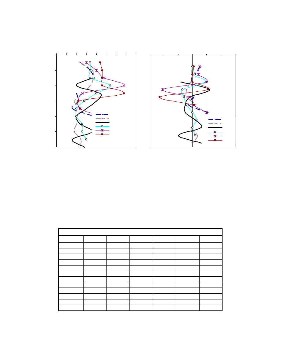
79
a.) Variation of Moisture Content
b.) Change of Moisture gradient
Fig. 3.18. (a) Variation of Moisture Content (MC) with Depth (z) and (b) Change of
Moisture Gradient with Depth (
ΔMC/Δz) (Project 3).
Table 3.14. Variation of Undrained Shear Strength with Depth in the Six Borings
(Project 3).
Depth (ft)
CCB-1
CCB-2
CCR-1
CCR-2
CCR-3
CCR-4
5
7
8.5
10
8.5
2
5
15
5.8
2.5
7.5
9
5
20
7
7
6
5
25
7.5
3
4
30
7.7
7.5
3
7
3
35
5.5
6.5
5
40
17.5
12
12
3
45
6.5
15
10
50
18
55
60
17
Undrained shear strength S
u
(psi)
0
10
20
30
40
50
60
10
15
20
25
30
35
40
45
50
Moisture Content (%)
D
ep
th
(ft)
CCB-2
CCB-1
CCR-1
CCR-2
CCR-3
CCR-4
0
10
20
30
40
50
60
-15
-10
-5
0
5
10
15
ΔMC / Δ z (%/ft)
D
ept
h (
ft
)
CCB-2
CCB-1
CCR-1
CCR-2
CCR-3
CCR-4
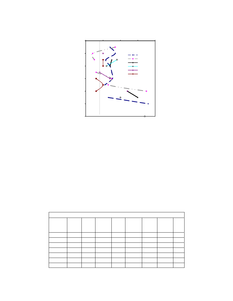
80
0
10
20
30
40
50
60
0
5
10
15
20
De
pth (f
t)
S
u
(psi)
CCB-1
CCB-2
CCR-1
CCR-2
CCR-3
CCR-4
Fig. 3.19. Variation of Undrained Shear Strength with Depth (Project 3).
• Consolidation properties (Project 3)
The consolidation parameters, summarized in Table 3.15, were obtained from the
standard incremental load consolidation test using samples from Boring CCR-3. Three
consolidation tests were performed on samples collected from depth of 14 - 15 ft, 18 -
19 ft, and 23 - 24 ft.
Table 3.15. Consolidation Parameters Used for the Settlement Estimation
(Project 3).
Settlement parameters
Depth
(ft)
Layers
height
(ft)
C
c
C
r
e
o
C
v Av
( in
2
/day)
σ
p
(psf)
σ
o
(psf)
OCR
2.5 5.0
0.199
0.050
0.66
1.128
1500
300
5.0
7.5 5.0
0.199
0.050
0.66
1.128
1500
875
1.7
12.5 5.0
0.199
0.050
0.66
1.128
1500
1188
1.3
18.5 7.0
0.377
0.038
1.06
0.522
2600
1564
1.7
26.0 8.0
0.149
0.012
0.59
1.404
2200
2033
1.1
34.0 8.0
0.149
0.012
0.59
1.404
2200
2534
0.9
42.0 8.0
0.149
0.012
0.59
1.404
2200
3035
0.7

81
The soil sample from the 14 - 15 ft depth had a void ratio (e
0
) of 0.66 and an
average compression (C
c
) and recompression indices (C
r
) of 0.199 and 0.050,
respectively, with a preconsolidation pressure of 1500 psf and an average coefficient of
consolidation of 1.128 in
2
/day. These parameters were used for the top 15 ft, divided into
three layers of 5 ft each (Table 3.15).
The soil sample at the 18 – 19 ft depth had a void ratio (e
0
) of 1.06 and average
compression and recompression indices of 0.377 and 0.038, respectively. The
preconsolidation pressure was 2,600 psf and an average coefficient of consolidation of
0.522 in
2
/day. Its settlement parameters were used for the 7-ft layer underlying the top
15 ft (Table 3.15).
Finally, the soil sample at the 23 – 24 ft depth had a void ratio of 0.59 and average
compression and recompression indices of 0.149 and 0.012, respectively, with an average
coefficient of consolidation of 1.404 in
2
/day. Its settlement parameters were used for the
bottom 24 ft divided into three layers of 8 ft each (Table 3.15).
• Stress Dependency Phenomena (C
c
)
The stress dependency of the compression index was investigated based on the
available data. The samples were loaded from 0.25 tsf to 12 tsf. The slope -de / dlog
σ
’
was determined for each load increment (Fig. 3.20(b)). The three samples showed similar
stress dependent patterns. The incremental compression index (C’
c
) increased with the
increasing stress from 0.25 tsf to 2.50 tsf, then decreased despite the increased stress to
5.50 tsf, and then increased with the increased stress up to 12 tsf. The conventional
compression index C
c
was determined and used in the settlement calculation
(Table 3.16).
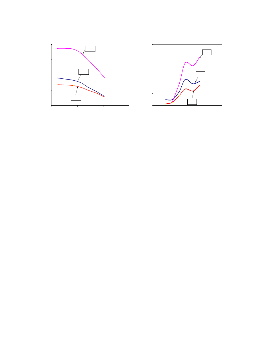
82
0.30
0.50
0.70
0.90
1.10
0.1
1
10
100
Vertical effective stress σ' (tsf)
Vo
id
r
at
io
e
23'-24'
14'-15'
18'-19'
`
0.00
0.10
0.20
0.30
0.40
0.50
0.1
1
10
100
Vertical effective stress σ' (tsf)
In
crem
en
ta
l C
c
23'-24'
14'-15'
18'-19'
a) b)
Fig. 3.20. (a) e – log
σ’ Relationship for the Three Samples and (b) Variation of
Compression Index with log
σ’ (Project 3).
• Stress Increase due to the embankment loading (Project 3)
The stress increase in the soil mass due to the embankment loading (
Δσ) was
calculated at the center and the toe of the embankment using the Osterberg method. A
surcharge of 240 psf was added to the total stress induced by the embankment, complying
with the TxDOT design method (Table 3.16). The average height of the embankment was
taken to be 9 ft.
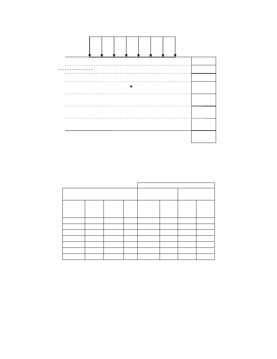
83
Fig. 3.21. Profile of the Soil Layers for Settlement Calculation (Project 3).
Table 3.16. Summary Stress Increase in the Soil Mass (Project 3).
Stress increase
Soil parameters
Center of the
embankment
Edge of the
embankment
Depth
(ft)
σ
p
(psf)
σ
o
(psf)
OCR
Center
Δσ
(psf)
σ
o
+
Δσ
(psf)
Εdge
Δσ
(psf)
σ
o
+
Δσ
(psf)
2.5 1500 300
5.0
1320 1620 0 300
7.5 1500 875 1.7 1319 2194 166 1041
12.5 1500 1188 1.3 1313 2501 292 1480
18.5 2600 1564 1.7 1297 2861 417 1981
26.0 2200 2033 1.1 1265 3298 475 2508
34.0 2200 2534 0.9 1216 3750 511 3045
42.0 2200 3035 0.7 1159 4194 531 3566
The variation of the stress increase with depth is shown in Fig. 3.22. The ratio of
the stress increase at the center to stress increase at the toe varied from infinite at the top
to 2.66 at the 26 ft depth.
W.T. 6.5 ft
CH
H (ft)
Δσ
CH 5
CH 7
CL 8
CH 5
CH 5
CH 7
CH 8
CL 7
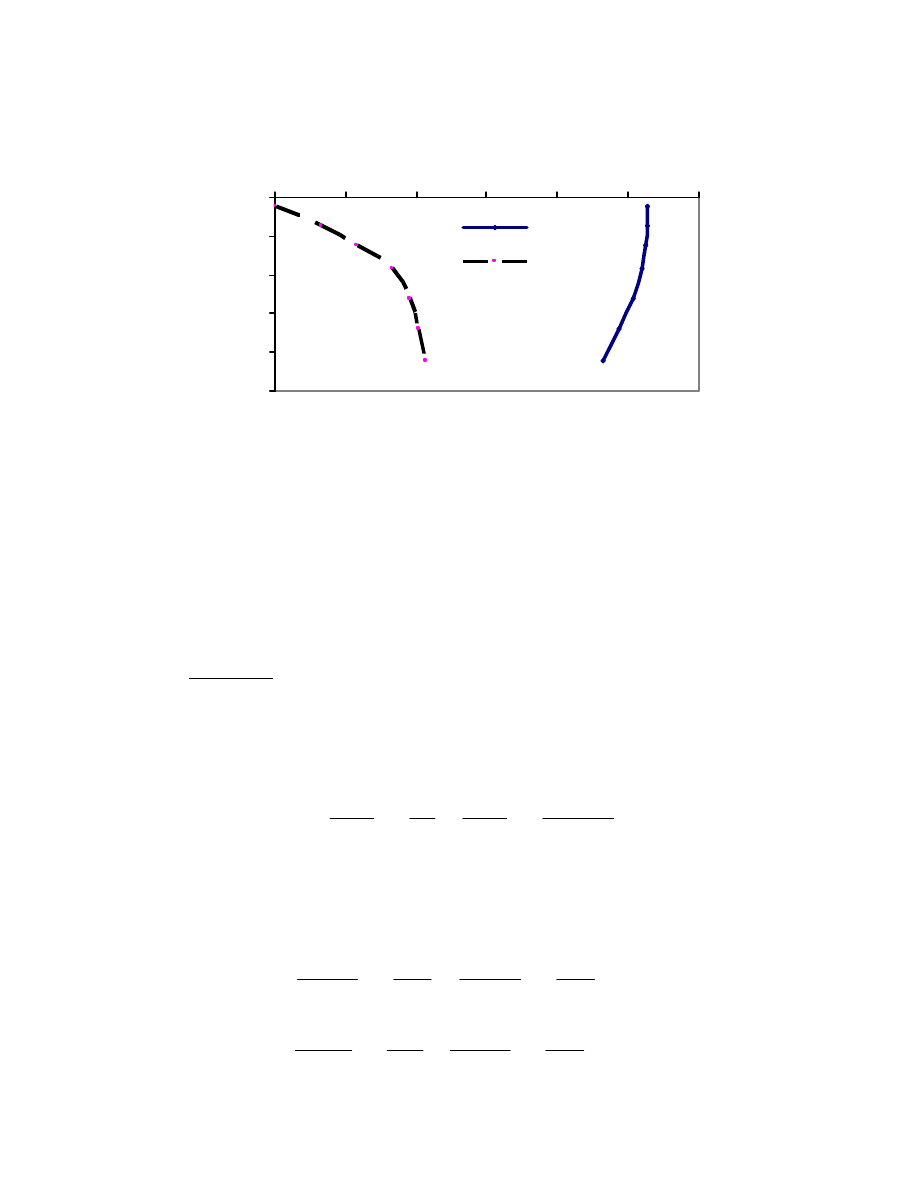
84
0
10
20
30
40
50
0
250
500
750
1000
1250
1500
Stress increase
Δσ (psf)
D
ept
h (ft
)
Center
Edge
Fig. 3.22. Variation of Stress Increase with Depth at the Center and at the Toe of the
Embankment Using the Osterberg Method (Project 3).
• Total settlement at the center (Project 3)
Based on the information provided by TxDOT, the total primary settlement was
8.50 in.
UH Check
: In all the layers, the total stress (
Δσ’ + σ’
o
) was higher than the
preconsolidation pressure (
σ
p
). Therefore, both the compression and recompression
indices were the governing parameters for the total primary settlement S
p
,
⎟
⎟
⎠
⎞
⎜
⎜
⎝
⎛
+
+
+
⎟
⎟
⎠
⎞
⎜
⎜
⎝
⎛
+
=
p
'
'
0
0
c
'
0
p
0
r
p
log
e
1
H
C
log
e
1
H
C
S
σ
σ
Δ
σ
σ
σ
. 2-12
Using the Osterberg method, the stress increase results at the center of the
embankment (Table 3.16), and the following results were obtained for 45 ft of soil:
Layer
1:
ft
1253
.
0
1500
1620
log
66
.
0
1
5
x
199
.
0
300
1500
log
66
.
0
1
5
x
05
.
0
S
p
=
⎟
⎠
⎞
⎜
⎝
⎛
+
+
⎟
⎠
⎞
⎜
⎝
⎛
+
=
Layer
2:
ft
x
x
S
p
1342
.
0
1500
2194
log
66
.
0
1
5
199
.
0
875
1500
log
66
.
0
1
5
05
.
0
=
⎟
⎠
⎞
⎜
⎝
⎛
+
+
⎟
⎠
⎞
⎜
⎝
⎛
+
=

85
Layer
3:
ft
1483
.
0
1500
2501
log
66
.
0
1
5
x
199
.
0
1188
1500
log
66
.
0
1
5
x
05
.
0
S
p
=
⎟
⎠
⎞
⎜
⎝
⎛
+
+
⎟
⎠
⎞
⎜
⎝
⎛
+
=
Layer
4:
ft
0817
.
0
2600
2861
log
06
.
1
1
7
x
377
.
0
1564
2600
log
06
.
1
1
7
x
038
.
0
S
p
=
⎟
⎠
⎞
⎜
⎝
⎛
+
+
⎟
⎠
⎞
⎜
⎝
⎛
+
=
Layer
5:
ft
1339
.
0
2200
3298
log
59
.
0
1
8
x
149
.
0
2033
2200
log
59
.
0
1
8
x
012
.
0
S
p
=
⎟
⎠
⎞
⎜
⎝
⎛
+
+
⎟
⎠
⎞
⎜
⎝
⎛
+
=
Layer
6:
ft
1276
.
0
2534
3750
log
59
.
0
1
8
x
149
.
0
S
p
=
⎟
⎠
⎞
⎜
⎝
⎛
+
=
Layer
7:
ft
0921
.
0
3035
4194
log
59
.
0
1
7
x
149
.
0
S
p
=
⎟
⎠
⎞
⎜
⎝
⎛
+
=
.
Hence the total primary settlement at the center of the embankment was
Sp = 0.1253 + 0.1342 + 0.1483 + .0817 + 0.1339 + 0.1276 + 0.1053 = 0.8431 ft
= 10.11 in.
The difference between the UH check result (10.11 in.) and the TxDOT
estimation (8.50 in.) was due to the thickness of soft soil considered for the settlement
estimation (Fig. 3.23). It was noted that if only the top 30 ft of soft soil was considered,
the total settlement would be 7.48 in.
• Rate of settlement at the center (Project 3)
TxDOT
The TxDOT rate of settlement estimation, using C
v
values in Table 3.15,
predicted a settlement of 5.10 in. after 1 year which represents 60% of the total primary
settlement (8.50 in.).

86
UH Check
: Using the TxDOT method, as described in Project 1A and 2, it was
considered that each clay layer had two drainage surfaces (top and bottom); the total
settlement reached in 2007, 14 years after construction, was determined as follows.
(a) Calculation
14 years = 168 months =14 x 365 = 5110 days
2
dr
v
v
H
t
c
T
=
2-13
(
)
(
)
[
]
179
.
0
8
.
2
v
5
.
0
v
/
T
4
1
/
T
4
100
%
U
π
π
+
=
(Das 2006).
3-1
Layer 1 to 3
(
)
(
)
⎯→
⎯
=
=
405
.
6
12
x
5
.
2
5110
128
.
1
T
2
v
U% = 99.7
Layer
4
(
)
(
)
⎯→
⎯
=
=
512
.
1
12
x
5
.
3
5110
522
.
0
T
2
v
U% = 97.31
Layer 5 to 7
(
)
(
)
⎯→
⎯
=
=
114
.
3
12
x
4
5110
404
.
1
T
2
v
U% = 99.46.
Consequently, the total settlement S
p168
after 14 years was
S
p168
= (0.997 x 0.1253) + (0.997 x 0.1342) + (0.997 x 0.1483) + (0.973 x 0.0817)
+ (0.994 x 0.1339) + (0.994 x 0.1276) + (0.994 x 0.0921)
= 0.8376 ft
= 10.05 in.
When considering the top 30 ft of soft clay layers,
S
p168
= 7.43 in.
Using the same calculation procedure, Fig. 3.23 was obtained.
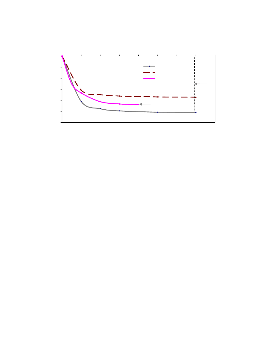
87
0
2
4
6
8
10
12
0
2
4
6
8
10
12
14
16
Settlem
ent (in)
Time ( years)
Soft soil :45 ft
Soft soil : 30 ft
TxDOT
TxDOT
2007
Fig. 3.23. Comparison of TxDOT Rate of Settlement Estimation at the Center of the
Embankment with New Estimation Using the Same Data.
Based on this procedure, more than 90% of the total settlement was completed in
1999, six years after construction in all three cases at the center of the embankment.
Consequently, the settlement of the embankment can be complete in 2007, 14 years later.
One-layer consideration
Method 1
Considering two drainage surfaces (top and bottom), the primary settlement
reached after 14 years (168 months), in 2007, was calculated using the following
procedure:
Weighted average of the coefficient of consolidation
(
) (
) (
)
day
/
in
175
.
1
45
404
.
1
x
23
522
.
0
x
7
128
.
1
x
15
H
H
C
C
2
i
i
vi
v
=
+
+
=
∑
∑
=

88
(
)
(
)
37
.
32
%
U
12
x
5
.
22
5110
175
.
1
H
t
c
T
2
2
dr
v
v
=
⎯→
⎯
=
=
=
S
p168
= 10.11 x 0.3237 = 3.27 in.
Based on this approach, the settlement reached in 2007 would be 3.27 in.,
representing about 32% of the total primary settlement at the center of the embankment.
When 30 ft of soft soil layers was considered, the total settlement 14 years later
was 48% (U= 0.484190) of the primary settlement and S
p168
= 3.58 in. After 15 years, the
50% total settlement (U=0.50093) will be S
p180
= 3.72 in. After 16 years the 51.7% total
settlement (U=0.51698) will be S
p180
= 3.84 in. Hence the expected consolidation
settlement under the center of the embankment in one year and two years after 14 years
will be 0.14 in. and 0.26 in., respectively.
Method 2
Considering two drainage surfaces (top and bottom), the necessary time to reach
90% of primary settlement can be calculated using the following procedure:
Weighted average of the coefficient of consolidation
day
/
in
175
.
1
C
2
v
=
.
With U% = 90%, T
v
= 0.848 and the time necessary time t is given by
(
)
day
52612
175
.
1
12
x
5
.
22
848
.
0
C
H
T
t
2
v
2
dr
v
=
=
=
= 144 years.
This result of 144 years was about 24 times what was predicted by the TxDOT
project approach (6 years) to reach 90% of the primary settlement at the center of the
embankment (Fig. 3.24).
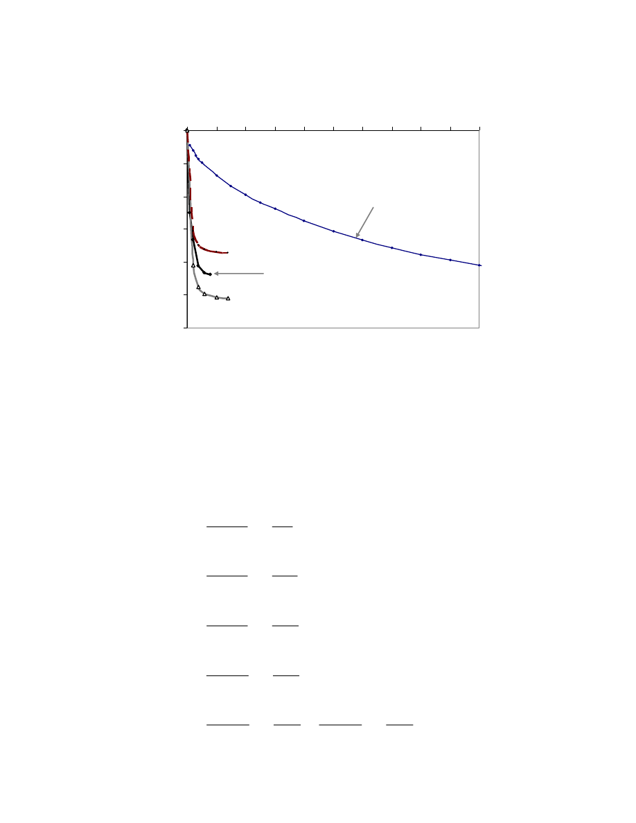
89
0
2
4
6
8
10
12
0
10
20
30
40
50
60
70
80
90
100
Time ( years)
S
ettle
me
nt
(in
)
T xDOT
1 layer
consideration
Fig. 3.24. Comparative Graph Showing the Effect of Layering on the Rate of
Settlement at the Center of the Embankment (Project 3).
• Total settlement at the toe (Project 3)
Using the Osterberg method, stress increase results at the toe of the embankment
(Table 3.16) and considering 45 ft of soft soil layers, the following results were obtained:
Layer
1:
ft
0
300
300
log
66
.
0
1
5
x
05
.
0
S
p
=
⎟
⎠
⎞
⎜
⎝
⎛
+
=
Layer
2:
ft
0114
.
0
875
1041
log
66
.
0
1
5
x
05
.
0
S
p
=
⎟
⎠
⎞
⎜
⎝
⎛
+
=
Layer
3:
ft
0144
.
0
.
0
1188
1480
log
66
.
0
1
5
x
05
.
0
S
p
=
⎟
⎠
⎞
⎜
⎝
⎛
+
=
Layer
4:
ft
0133
.
0
1564
1981
log
06
.
1
1
7
x
038
.
0
S
p
=
⎟
⎠
⎞
⎜
⎝
⎛
+
=
Layer
5:
ft
0447
.
0
2200
2508
log
59
.
0
1
8
x
149
.
0
2033
2200
log
59
.
0
1
8
x
012
.
0
S
p
=
⎟
⎠
⎞
⎜
⎝
⎛
+
+
⎟
⎠
⎞
⎜
⎝
⎛
+
=

90
Layer
6:
ft
0598
.
0
2534
3045
log
59
.
0
1
8
x
149
.
0
S
p
=
⎟
⎠
⎞
⎜
⎝
⎛
+
=
Layer
6:
ft
0459
.
0
3035
3566
log
59
.
0
1
7
x
149
.
0
S
p
=
⎟
⎠
⎞
⎜
⎝
⎛
+
=
.
Hence the total primary settlement at the toe of the embankment was
Sp = 0 + 0.0114 + 0.0144 + 0.0133 + 0.0477 + 0.0598 + 0.0459 = 0.1895 ft
= 2.27 in.
Hence the total settlement 14 years later was 32% (U= 0.3237) of the primary settlement
and S
p168
= 0.73 in. After 15 years, the 33.5% total settlement (U=0.3351) will be S
p180
=
0.76 in. After 16 years, the 34.6% total settlement (U=0.3460) will be S
p180
= 0.79 in.
Hence the expected consolidation settlement in the edge of the embankment in one year
and two years after 14 years will be 0.03 in. and 0.06 in., respectively.
Considering 30 ft of soft clay layer, S
p (toe)
= 1.01 in. The total settlement 14 years
later was 48% (U= 0.484190) of the primary settlement occurs and S
p168
= 0.48 in. After
15 years, the 50% total settlement (U=0.50093) will be S
p180
= 0.50 in. After 16 years, the
51.7% total settlement (U=0.51698) will be S
p180
= 0.52 in. Hence the expected
consolidation settlement in the edge of the embankment in one year and two years after
14 years will be 0.02 in. and 0.04 in., respectively.
• Rate of settlement at the toe (Project 3)
Using the same procedure used to calculate the rate of settlement at the center of
the embankment, Fig. 3. 25 and Fig. 3.26 were obtained. Ninety percent of the total
settlement (2.04 in.) was reached at the toe of the embankment four years after
construction using the TxDOT method. After 14 years in 2007, 99.6% (2.26 in.) of the
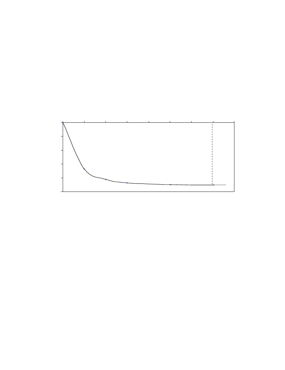
91
total settlement was reached. Therefore, based on this method, the primary settlement is
considered over (Fig. 3.26).
When one layer was assumed for the soft soil, the resulting rate of settlement
predicted 32.3% of the total settlement at the toe (0.73 in.), which was reached in 2007. It
was three times less than the one obtained by using the TxDOT method (Fig. 3.26).
Fig. 3.25. Rate of Settlement at the Toe of the Embankment Using TxDOT Method.
Soft soil :45 ft
0.0
0.5
1.0
1.5
2.0
2.5
0
2
4
6
8
10
12
14
16
Time ( year)
Se
ttl
em
en
t (i
n)
2007
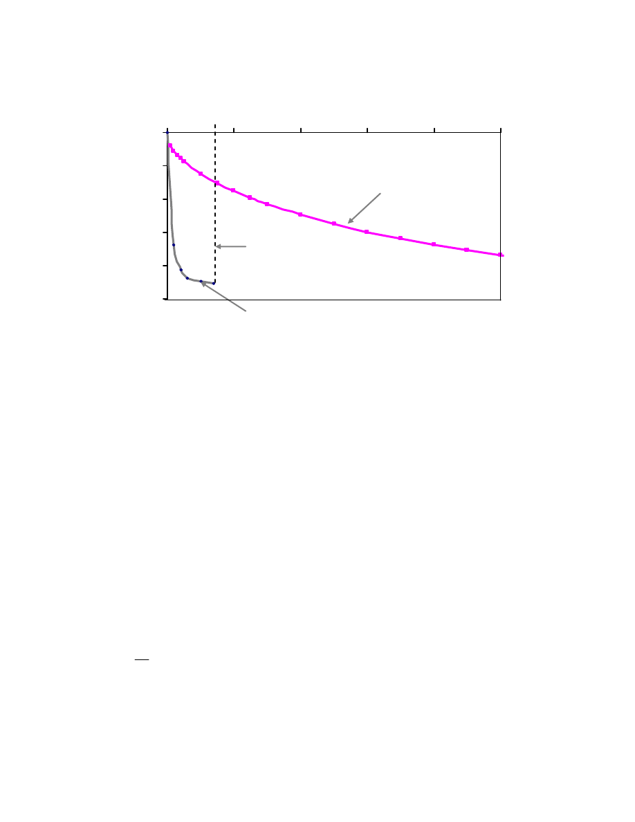
92
0.0
0.5
1.0
1.5
2.0
2.5
0
20
40
60
80
100
Time ( year)
Se
ttle
m
en
t (
in
)
2007
1 layer
consideration
TxDOT method
Fig. 3.26. Comparative Graph Showing the Effect of Layering on the Rate of
Settlement at the Toe of the Embankment.
• Excess Pore Water Pressure
Considering the 14 years of the embankment in place, we have the following
consideration:
u
o
= initial excess pore water pressure at the construction of the embankment in 1993
u
i
= excess pore water pressure at a specific time t.
In Section 3.2.6, by considering one layer of soft soil and two drainage surfaces
and the consolidation parameters of 1991, it was ascertained that 32.37% of the
consolidation (total thickness of 45 ft) was completed in 2007.
o
i
o
i
u
676
.
0
u
324
.
0
u
u
1
U
=
⎯→
⎯
=
−
=
.
Assuming that u
o
=
Δσ
’
,
the remaining excess pore water pressure u
i
is given by
u
i
= 0.676u
o
= 0.676
Δσ
’

93
Using the increase in stress due to the embankment at the 26 ft depth below the
toe of the embankment the pore water pressure is 475 psf (Table 3.16). Hence the excess
pore water pressure will be 2.23 psi.
If the total thickness was 30 ft, then the pore water pressure will be 0.516
Δσ
’.
Hence the excess pore water pressure will be 1.70 psi.
Comment on the settlement prediction (Project 3)
- All the predictions were based on three consolidation tests. These three tests
were representing 45 ft of soil. The number of tests is not representative of the
variability in deltaic soil deposits. At least one consolidation test should be
done every 6 ft of depth to better estimate the consolidation properties.
- The method used to estimate the stress increase was closer to the Osterberg
method. The soft clay soil was overconsolidated, and in all six layers the total
effective stress was higher than the preconsolidation pressure. Therefore, both
compression and recompression indices are governing parameters of the total
primary settlement. The type of the recompression index used for the
calculation was not clear.
- The TxDOT project approach used layers of soft soils to estimate the time of
settlement. This approach underestimated the time of settlement and is not
correct based on theory because of the assumed drainage condition for each
layer.

94
3.1.6.
Project No 4 (NASA Road 1 @ Taylor Lake)
At the time of review of the data in 2007, the highway embankment had been in
service for seven years. The designed embankment height varied from 10 to 15 ft, and the
base width (W) was 60 ft (Fig. 3.27). The ratio W
H
varied then from 0.17 to 0.25. About
11 borings were taken on site to collect the geotechnical information from 1994 through
2007 for construction, and monitoring of the road as follow:
- Three borings (TB-1, TB-2, and TB-3) were drilled in March 1994.
TCP (Texas Cone Penetrometer) tests were conducted during the drilling and
soil samples were taken for laboratory testing. The embankment and the
bridge were both constructed in September 2000.
- In April 2005, due to the observed embankment settlements four more borings
were drilled for further investigation (AT-1, AT-2, AT-3, and AT-4). Prior to
asphalt patching in 2006, 1 to 2.5 inches of elevation difference was measured
between bridge and embankment sides.
- In April 2007, four boreholes (UH-1, UH-2, UH-3, and UH-4) located along
the embankment, were drilled on the roadway (Fig 3.28). During drilling, the
TCP blow counts were recorded to determine the consistency of the soil along
the depth.
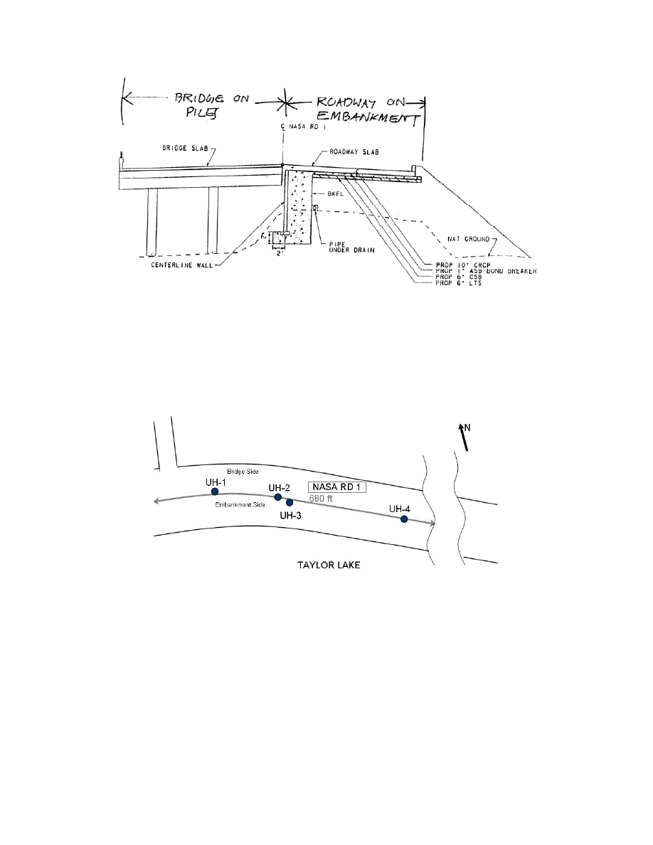
95
Fig. 3.27. Cross Section of the Bridge and the Embankment at Nasa Road 1 Site.
Fig. 3.28. Approximate Borehole Locations Drilled in April 2007 (Not to Scale).
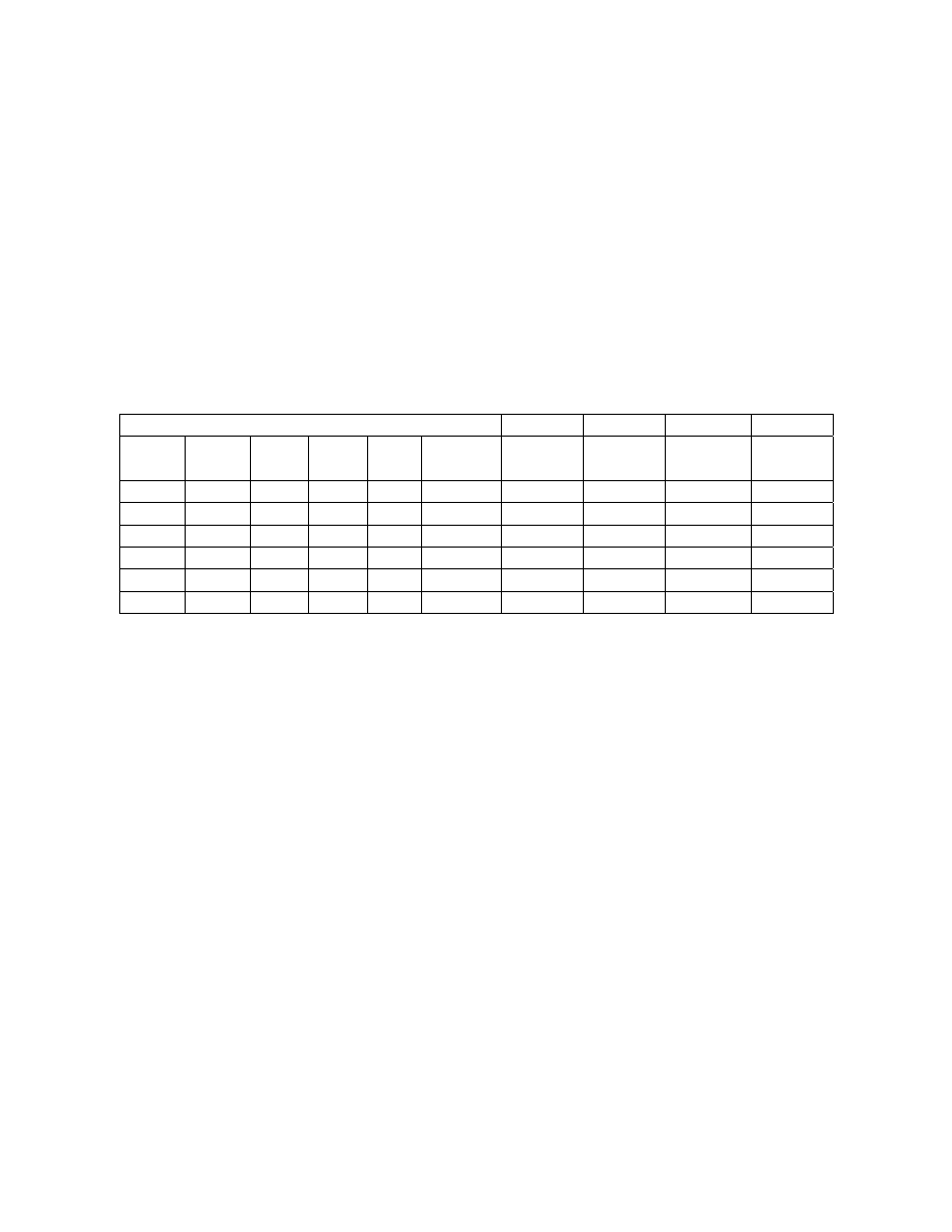
96
• Stress Increase due to the embankment loading (Project 4)
The stress increase in the soil mass due to the embankment loading (
Δσ) was
calculated at the center and the toe of the embankment using the Osterberg method. A
surcharge of 240 psf was added to the total stress induced by the embankment, complying
with the TxDOT design method (Table 3.17). The average height of the embankment was
taken to be 20 ft.
Table 3.17. Summary of Stress Increase in the Soil Mass.
Soil Parameters
Center
Edge
Center
Edge
Depth e
o
Cc Cr
σ
p
(psf)
σ
o
(psf)
Δσ
(psf)
Δσ
(psf)
σ
o
+Δσ
(psf)
σ
o
+Δσ
(psf)
1.5 0.618 0.2 0.04
4800
93.6 2741 108 2834 202.
6.5 0.618 0.2 0.04
4800
405.6 2725 433 3131 838
12.5 0.618 0.2 0.04 4800
780 2648
702
3428 1482
17.5 1.329 0.26 0.01 3400
1092 2531
844
3623 1936
30 0.656 0.126 0.062 4000
1872
2143
1067
4015.
2939
52.5 0.85 0.241 0.061 3800
3276
1536
1129
4812
4405
The variation of the stress increase with depth is shown in Fig. 3.29. The ratio of
the stress increase at the center to stress increase at the toe varied from 25.3 near the top
to 1.36 at the 52.5 ft depth.
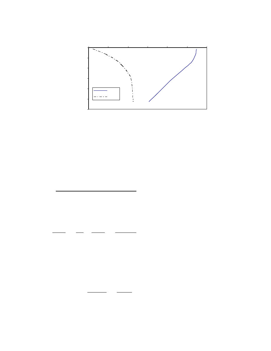
97
0
10
20
30
40
50
60
0
500
1000
1500
2000
2500
3000
Stress increase Δσ (psf)
D
ep
th (ft)
Center
Edge
Fig. 3.29. Variation of Stress Increase with Depth at the Center and at the Toe of the
Embankment Using the Osterberg Method (Project 4).
• Total settlement at the center (Project 4)
Based on the information provided by TxDOT, the total primary settlement was
37.87 in.
UH Check (total thickness of 65 ft)
: In three layers, the total stress (
Δσ’ + σ’
o
)
was higher than the preconsolidation pressure (
σ
p
). Therefore, both the compression and
recompression indices were the governing parameters for the total primary settlement S
p
,
⎟
⎟
⎠
⎞
⎜
⎜
⎝
⎛
+
+
+
⎟
⎟
⎠
⎞
⎜
⎜
⎝
⎛
+
=
p
'
'
0
0
c
'
0
p
0
r
p
log
e
1
H
C
log
e
1
H
C
S
σ
σ
Δ
σ
σ
σ
Using the Osterberg method, the stress increase results at the center of the
embankment (Table 3.17), and the total primary settlement at the center of the
embankment was calculated as follows
Layer
1:
.
32
.
1
6
.
93
8
.
2834
log
618
.
0
1
3
04
.
0
in
x
S
p
=
⎟
⎠
⎞
⎜
⎝
⎛
+
=

98
Layer
2:
.
84
.
1
6
.
405
5
.
3131
log
618
.
0
1
7
04
.
0
in
x
S
p
=
⎟
⎠
⎞
⎜
⎝
⎛
+
=
Layer
3:
.
95
.
0
780
4
.
3428
log
618
.
0
1
5
04
.
0
in
x
S
p
=
⎟
⎠
⎞
⎜
⎝
⎛
+
=
Layer
4:
.
31
.
0
3400
5
.
3623
log
329
.
1
1
5
26
.
0
1092
3400
log
329
.
1
1
5
01
.
0
in
x
x
S
p
=
⎟
⎠
⎞
⎜
⎝
⎛
+
+
⎟
⎠
⎞
⎜
⎝
⎛
+
=
Layer
5:
.
99
.
2
4000
2
.
4015
log
656
.
0
1
20
126
.
0
1872
4000
log
656
.
0
1
20
062
.
0
in
x
x
S
p
=
⎟
⎠
⎞
⎜
⎝
⎛
+
+
⎟
⎠
⎞
⎜
⎝
⎛
+
=
Layer
6:
.
65
.
4
3800
9
.
4812
log
85
.
0
1
25
241
.
0
3276
3800
log
85
.
0
1
25
061
.
0
in
x
x
S
p
=
⎟
⎠
⎞
⎜
⎝
⎛
+
+
⎟
⎠
⎞
⎜
⎝
⎛
+
=
S
p
=1.32 in. + 1.84 in. + 0.95 in. + 0.31 in. + 2.99 in. + 4.65 in. = 12.06 in.
The difference between the UH check result (12.06 in.) and the TxDOT
estimation (37.86 in.) was due to the fact that overconsolidation of the layers were taken
into account in the UH approach in addition to the recompression index, C
r
, for the
settlement estimation. If only the top 10 ft thickness of the soft soil was considered, the
total primary settlement at the center of the embankment would be 4.1 in. The
consolidation settlement for the top 20 ft thickness of soft soil would be 4.43 in. It must
be noted that these depths were analyzed because the embankment was instrumented to
these two depths.
Rate of Settlement (Project 4)
One-layer consideration
Considering two drainages surfaces (top and bottom), the primary settlement
reached after 7 years (84 months), in 2007, was calculated using the following procedure:
Weighted average of the coefficient of consolidation

99
sec
/
10
97
.
1
2
4
in
x
C
v
−
=
(
)
(
)
72
.
59
%
12
5
.
32
10
21
.
2
10
97
.
1
2
8
4
2
=
⎯→
⎯
=
=
=
−
U
x
x
x
H
t
c
T
dr
v
v
S
p84
= 4.43 x 0.5972 = 2.64 in.
Based on this approach, the settlement reached in 2007 (after 7 years) for 20 ft
thickness of the soil would be 2.64 in., representing about 59.7% of the total primary
settlement at the center of the embankment. After 8 years, U =0.6356 and total settlement
was 63.5% with the settlement being S
p96
= 2.81 in. Hence, the expected consolidation
settlement in the center of the embankment in one year (between 7 and 8 years) would be
0.17 in. in the 20-ft thick layer.
The settlement reached in 2007 (U=0.5972) in the top 10-ft thickness of the soft
soil would be 2.49 in. After 8 years the settlement will be 63.5% of the total settlement
(U=0.6356) and would be S
p96
= 2.01 in. Hence the expected consolidation settlement in
the 10-ft thick top layer center of the embankment in one year will be 0.12 in.
In Fig. 3.30 the rate of settlement predicted by TxDOT and UH approaches are
compared. The time required for 99% of the consolidation as predicted by UH was
43.6 years. Based on the TxDOT calculations the time required for 99% of the
consolidation was 38.4 years.
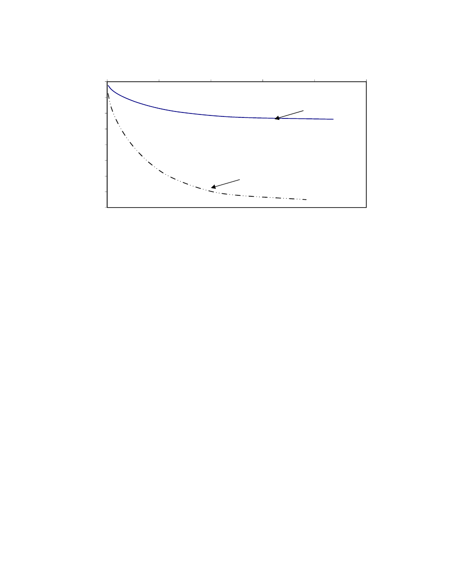
100
0
5
10
15
20
25
30
35
40
0
10
20
30
40
50
Settl
emen
t (i
n
)
Time (Years)
UH
TxDOT
Fig. 3.30. Comparison of Rate of Settlement (Project 4).
3.2.
Summary and Discussion
A total of four TxDOT projects were reviewed to ascertain the procedures used by
TxDOT to predict the settlement of embankments on soft soils. Based on the review of
the design and analyses the following observations can be advanced:
(1) The method currently used in TxDOT projects to determine the increase in in-situ
stress is comparable to the Osterberg method and is acceptable. The approach
used in TxDOT projects to determine the preconsolidation pressure is acceptable
(Casagrande Method).
(2) The total settlement has been estimated in TxDOT projects based on very limited
consolidation tests. Since the increase in in-situ stresses due to the embankment
are relatively small (generally less than the preconsolidation pressure), using the
proper recompression index is import. Reviewing of the TxDOT project

101
approaches indicates that there is no standard procedure to select the
recompression index.
(3) The procedure used in TxDOT projects to determine the rate of settlement is not
acceptable. In determining the rate of settlement, the thickness of the entire soil
mass must be used with the average soil properties and not the layering method.
The layered approach will not satisfy the drainage conditions needed to use in the
time factor formula and determine the appropriate coefficient of consolidation.
(4) The consolidation index (C
c
) was stress dependent. Hence, when selecting
representative parameters for determining the total settlement, expected stress
increases in the ground should be considered.
(5) The number of consolidation tests used to determine the consolidation properties
of the soils in each project must be increased. Due to the variability in properties
of deltaic deposited clay soils, it is recommended to use one consolidation test for
each 6 ft depth of soil used for settlement analyses.

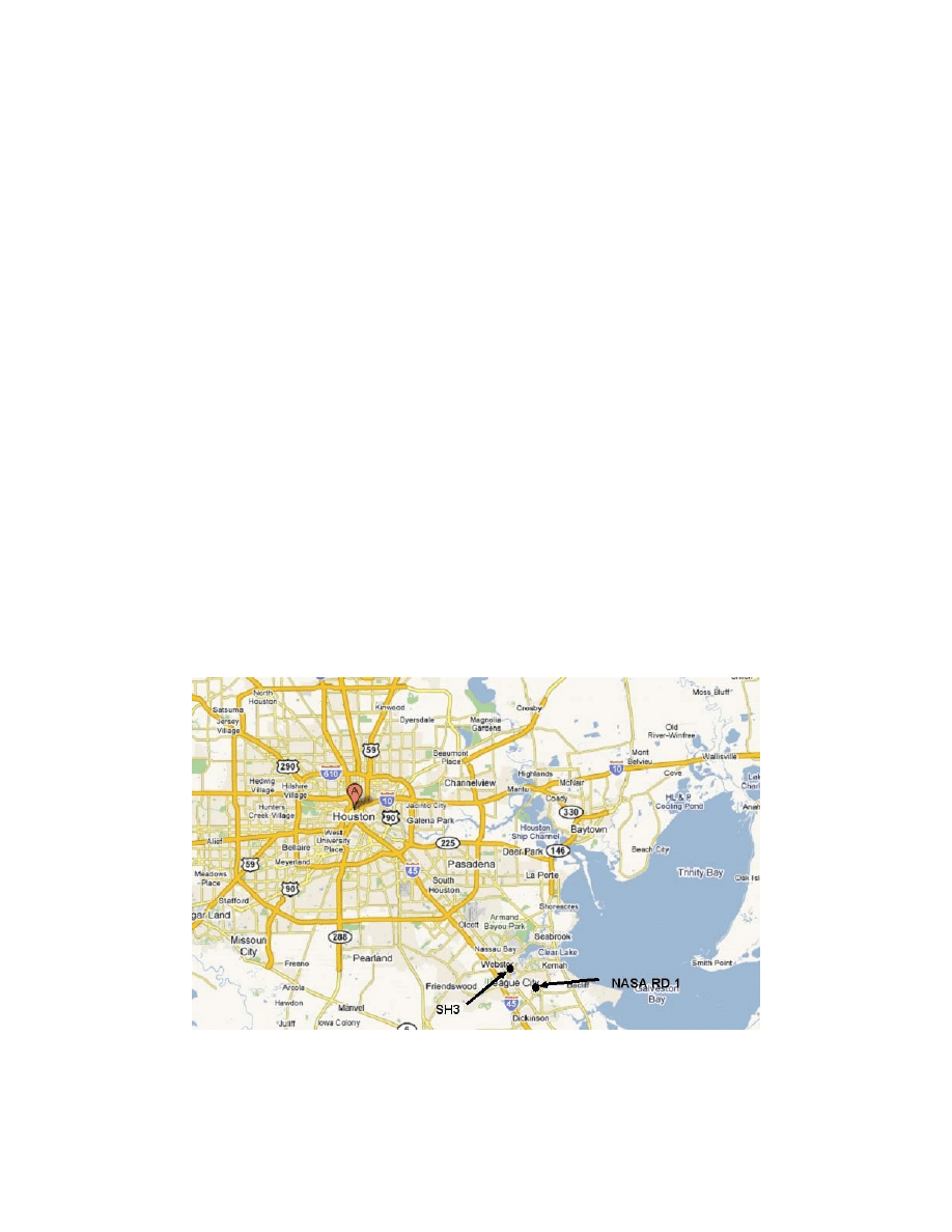
103
4. LABORATORY
TESTS AND ANALYSIS
4.1. Introduction
Soil samples were collected from SH3 at Clear Creek (CSJ 0051-03-069) and
NASA Road 1 at Taylor Lake (CSJ 0981-01-104) (Fig. 4.1) for laboratory study. Shelby
tubes, 3 inches in diameter and 30 in. in length, with an average area ratio of 9.5% were
used to collect the soil samples. While some samples were extruded, wrapped in
aluminum foil, put in transparent plastic bags and stored in 3’’ by 6’’ or 3’’ by 12’’
containers for index tests, others remained in the Shelby tubes for use in consolidation
and strength tests. Samples were stored vertically in plastic buckets and transported to the
University of Houston’s Geotechnical Laboratory for testing. Information on the
collected samples is summarized in Table 4.1. In addition to performing standard
geotechnical tests, soil samples were used to perform a limited amount of constant rate of
strain (CRS) tests to determine the consolidation parameters.
Fig. 4.1. Location of the Two Field Sites in Houston, Texas.
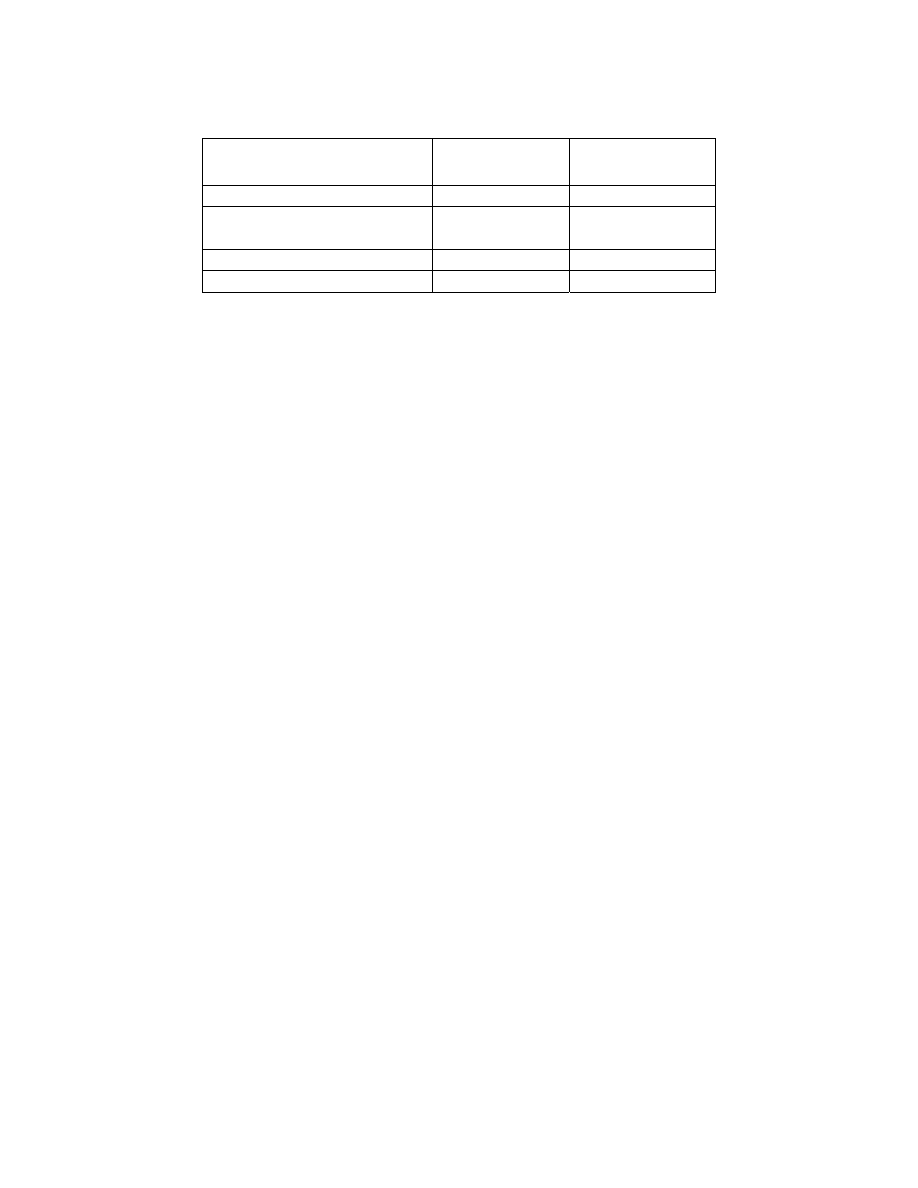
104
Table 4.1. Summary of the Samples Collected.
Details SH3
NASA
Rd.
1
Depth of Samples (ft)
20 to 30
30 to 50
Number of Samples
Collected
56 20
Total Number of Boreholes
5
4
Total Length of Samples (in)
876
282
4.2. Tests
Results
A series of soil tests included index properties, consolidation, and unconfined
compressive strength.
4.2.1.
SH3 at Clear Creek site
• Natural moisture content: A total of 50 moisture content (MC) tests were
performed to determine the variation of MC with depth in all five borings
(Fig. 4.2). The highest MC was 60.8% in the CH soil at a depth of 17 ft in
Borehole B4. The lowest MC was 18.7% in the CH soil at a depth of 3 ft in
Borehole B2. The highest change was observed between 10 and 20 ft
(representing a change in moisture content of 25%) and it was also represented by
the transition from the CH to the CL clay soil. The minimum and maximum MCs
reported by TxDOT based on the tests done in early 1990s and before were 18%
and 44%, respectively. The maximum MC of 44% was in the CH soil at a depth
of 20 to 25 ft. This is also an indication of the variability that can be expected in a
deltaic deposit (Vipulanandan et al. 2007).
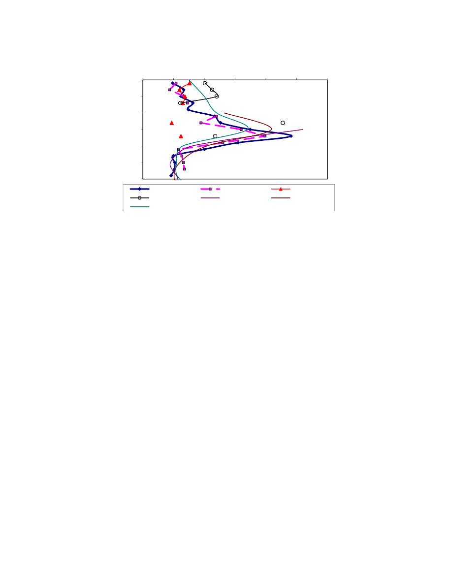
105
0
5
10
15
20
25
30
10
20
30
40
50
60
70
De
pth (
ft)
Moisture Content (%)
B1
B2
B3
B4
Old data M1
Old data R2
Old Data CCR-3
Fig. 4.2. Variation of Moisture Content with Depth in All the Boreholes (SH3).
• Liquid limit: A total of 27 liquid limit (LL) tests were performed to determine
the type of clay soil and its variation with depth (Fig. 4.3). The highest LL was
91% in the CH soil at a depth of 15 ft. The lowest LL was 27.4% in the CL soil
at a depth of 11 ft. Previous study based on 97 data sets on soft deltaic clay soils
in this region showed that the LL varied from 24% to 93% with a mean of
53.6%, standard deviation of 22.7%, and coefficient of variation of 2.36%
(Vipulanandan et al. 2007). Hence the data from the four boreholes were within
the range reported in the literature.
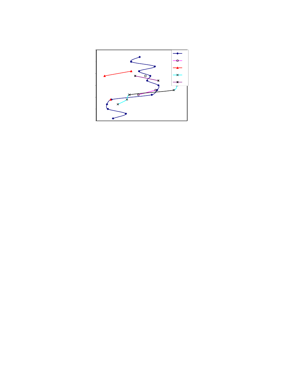
106
0
5
10
15
20
25
30
20
40
60
80
100
De
pth (
ft)
Liquid Limit (%)
B1
B2
B3
B4
B5
Fig. 4.3. Variation of Liquid Limit with Depth (SH3).
• Plastic limit: A total of 27 plastic limit (PL) tests were performed to determine
the type of clay soil and its variation with depth in boreholes (Fig 4.4). The
highest PL was 24.6% in the CH soil at a depth of 13 ft. The lowest PL was
15.3% in the CL soil at a depth of 27 ft. Previous study based on 97 data sets on
soft deltaic clay soils in this region showed that the LL varied from 8 to 35%
with a mean of 21.8%, a standard deviation of 6.9%, and coefficient of variation
of 31.6% (Vipulanandan et al. 2007). Hence the data from the four boreholes
were within the range reported in the literature.
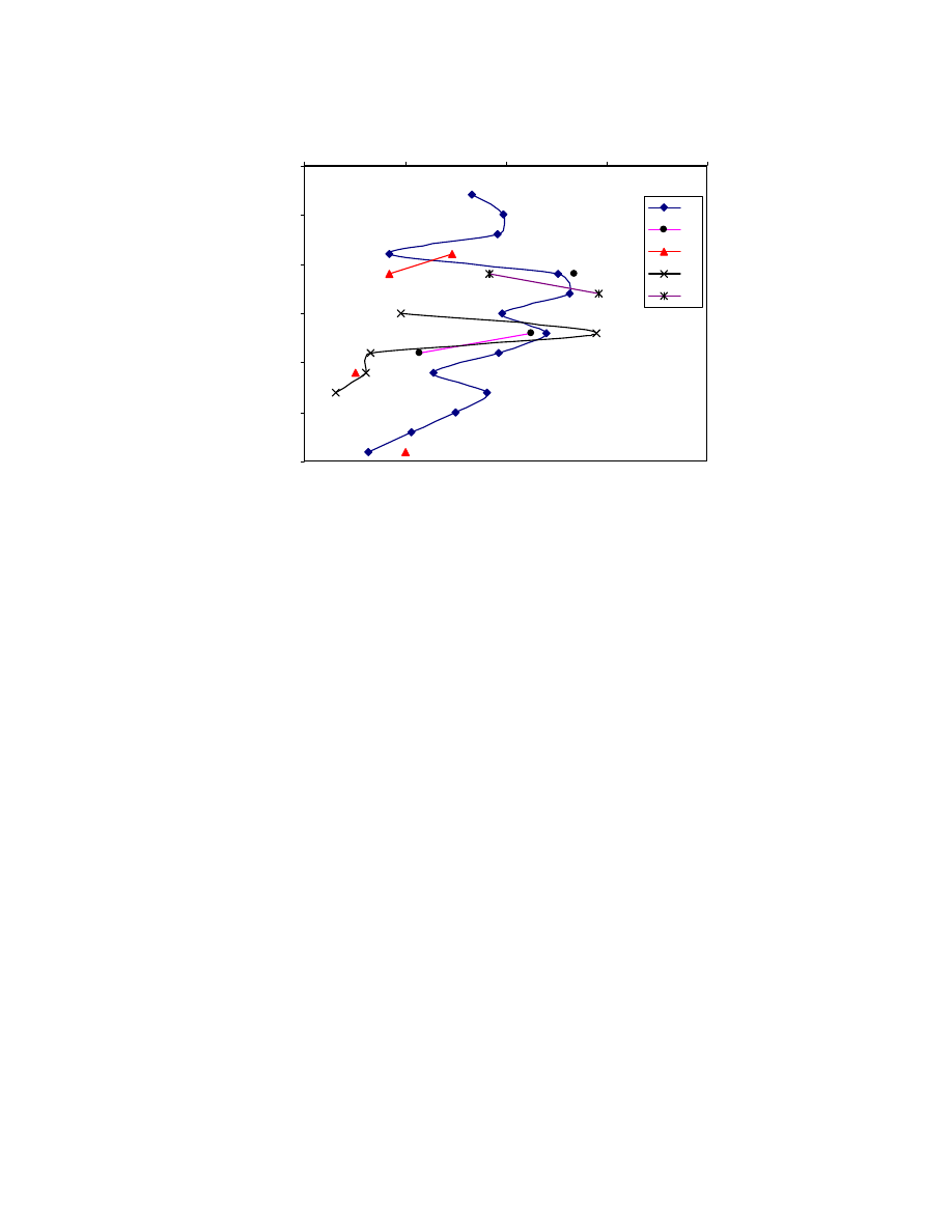
107
0
5
10
15
20
25
30
10
15
20
25
30
Plastic Limit (%)
D
ep
th
(ft)
B1
B2
B3
B4
B5
Fig. 4.4. Variation of Plastic Limit with Depth in Boring B1 (SH3).
• Undrained shear strength (S
u
): A total of 26 undrained shear strength tests were
performed to determine the strength of the soil and its variation with depth in four
the four boreholes (Table 4.3 and Fig. 4.5). The highest S
u
was 17.7 psi in the CH
soil at a depth of 7 ft in Boring B3. The lowest S
u
was 2.14 psi in the CH soil at a
depth of 17 ft in Boring B4. The undrained shear strength from previous testing at
this location varied from 2 psi to 18 psi (Table 3.14). The variation in the strength
results is comparable.
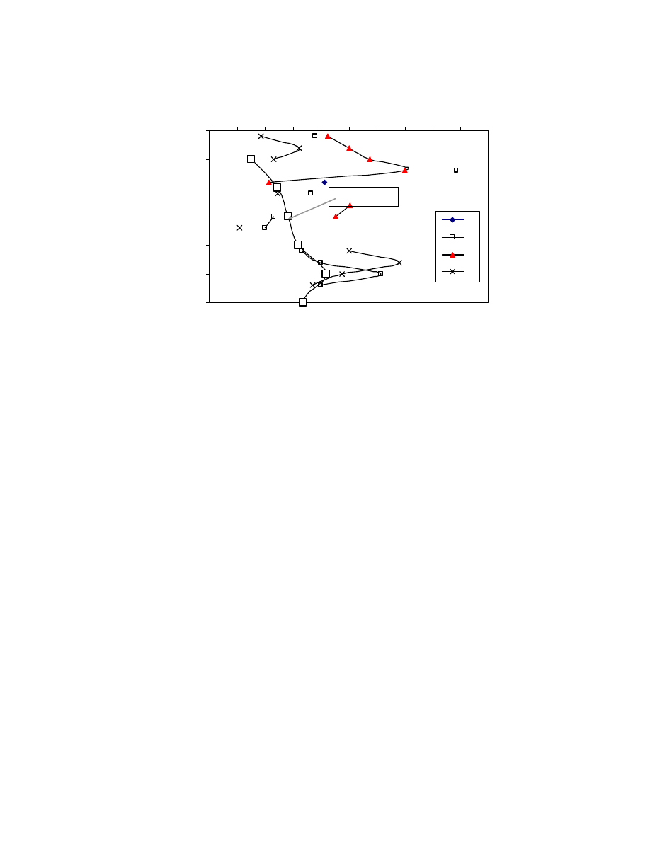
108
0
5
10
15
20
25
30
0
2
4
6
8
10
12
14
16
18
20
SH3 Undrained shear strength (psi)
De
p
th
(ft
)
B1
B2
B3
B4
1984 data
Fig. 4.5. Variation of S
u
with Depth in Borings B1, B2, B3, and B4 (SH3).
• Overconsolidation ratio (OCR): A total of 27 incremental load (IL)
consolidation tests were performed, and the overconsolidation ratio variation with
depth in Borehole B1 is summarized in Table 4.4 and plotted in Fig. 4.6. The
highest OCR was 9.6 in the CH soil at a depth of 3 ft in boring. The lowest OCR
was 1 in the CL soil at a depth of 25 and 29 ft. The clay soil was overconsolidated
(OCR > 1) up to 23 ft in CH clay soil. The OCR from previous testing at this
location varied from 1 to 5 (Table 3.15). Although the magnitudes were somewhat
different, the variation in the OCR with depth was comparable.
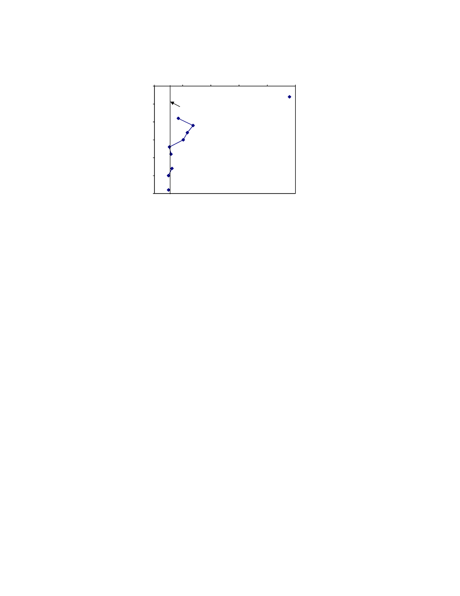
109
0
5
10
15
20
25
30
0
2
4
6
8
10
D
ep
th
(ft)
OCR
OCR=1
Fig. 4.6. Variation of Overconsolidation Ratio with Depth in Borehole B1 (SH3).
• Compression index (C
c
): A total of 10 compression indices were determined
from 10 IL consolidation tests on samples from Boring B1 (Table 4.4), and their
variation with depth is shown in Fig. 4.7. The highest C
c
was 0.446 in the CH soil
at a depth of 17 ft. The lowest C
c
was 0.086 in the CL soil at a depth of 23. The
minimum and maximum C
c
reported by TxDOT based on the tests done in the
early 1990s and before were 0.149 and 0.377, respectively (based on three
consolidation tests). There was an 18% difference in the maximum C
c
.
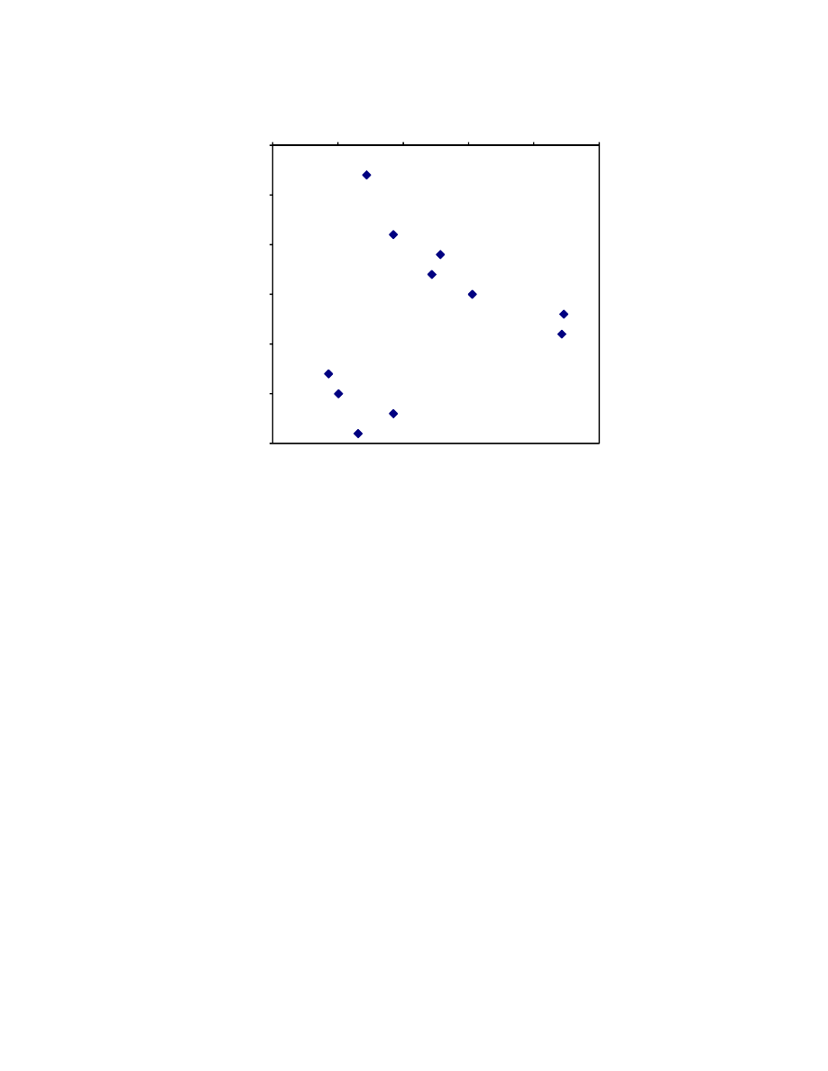
110
0
5
10
15
20
25
30
0.0
0.1
0.2
0.3
0.4
0.5
De
pth (f
t)
Compression Index Cc
Fig. 4.7. Variation of Compression Index with Depth in Boring B1 (SH3).
• Recompression index (C
r
): A total of 28 recompression indices of three types
(C
r1
, C
r2
, and C
r3
) were determined from 10 IL consolidation tests on samples
from Borehole B1 (Table 4.4). The different types of recompression indices were
introduced and discussed in Section 4.6.1. The minimum and maximum C
r
reported by TxDOT based on the tests done in the early 1990s and before were
0.012 and 0.050, respectively, and were comparable to the C
r1
of the current
study.
• Coefficient of consolidation (C
v
): A total of seven coefficients of consolidation
were determined from seven IL consolidation tests on samples from Borehole B1
(Table 4.4), and their variation with depth is shown in Fig. 4.8. The highest C
v
was 24.90 in
2
/day in the CL soil at a depth of 29 ft. The lowest C
v
was
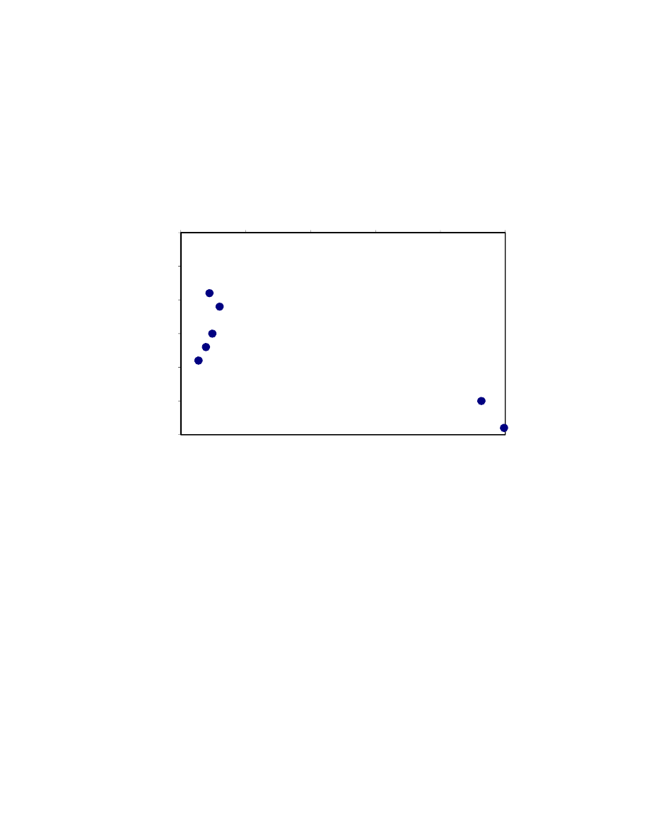
111
1.37 in
2
/day in the CH soil at a depth of 19 ft. The minimum and maximum C
v
reported by TxDOT based on the tests done in the early 1990s and before were
0.522 in
2
/day and 1.404 in
2
/day, respectively (Table 3.15). The difference in C
v
will affect the rate and total time for consolidation.
0
5
10
15
20
25
30
0
5
10
15
20
25
De
pth (f
t)
Coefficient of consolidation (Cv) (in2/day)
Fig. 4.8. Variation of Coefficient of Consolidation with Depth in Borehole B1 (SH3).
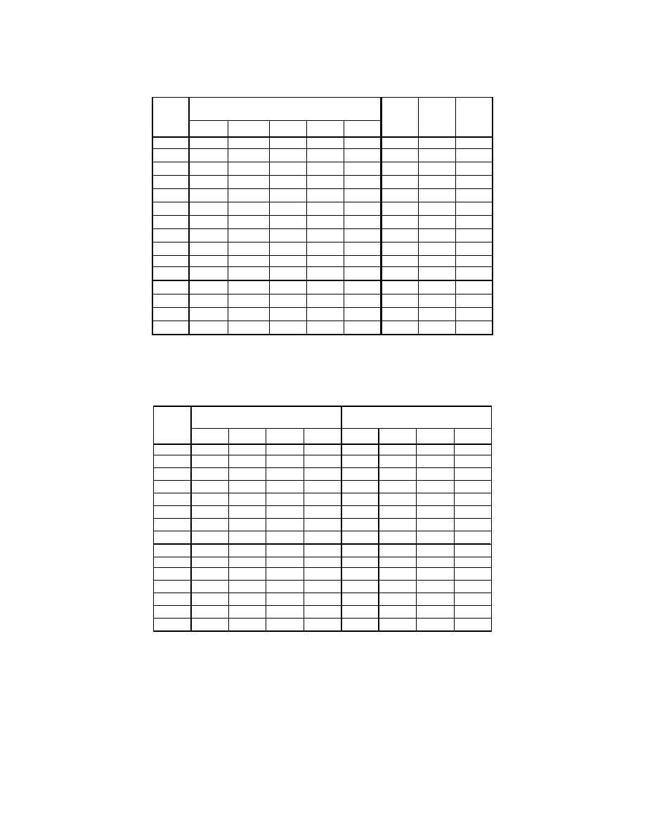
112
Table 4.2. Summary of Soil Type Parameters (SH3).
B1
B2
B3
B4
B5
1
19.7
20.8
25.2
34.6
30.2
3
23.3
18.7
21.9
29.7
32.5
58.2
18.3
CH
5
22.4
23.4
23.7
31.8
34.0
50.7
19.9
CH
7
26.3
24.5
23.0
27.0
22.2
71.5
19.6
CH
9
24.8
11
33.3
33.9
35.7
67.5
22.6
CH
13
35.3
28.9
19.4
52.9
55.5
64.8
23.2
CH
15
44.9
42.0
75
19.8
CH
17
58.2
49.7
22.4
60.8
33.5
73.5
22
CH
19
36.0
21
30.0
21.6
22.3
33.5
16.4
CL
23
19.9
22.7
29.5
19.1
CL
25
20.4
23.2
21.5
30.3
17.5
CL
27
20.3
23.5
23.3
46.1
15.3
CL
29
19.2
TYPE
Depth
(ft)
MC (%)
LL (%)
B1
PL (%)
B1
Table 4.3. Summary of Strength Parameters (SH3).
B1
B2
B3
B4
B1
B2
B3
B4
1
131.0
127.2
125.0
114.8
7.60
8.50
3.70
3
128.7
125.1
126.1
121.1
10.00
6.45
5
132.6
133.7
133.4
115.4
11.50
4.63
7
126.4
134.7
131.6
17.70
14.00
9
123.0
128.7
116.0
8.25
4.30
11
120.5
122.7
121.9
7.32
4.89
13
116.8
124.4
138.8
10.08
15
116.0
115.0
151.8
4.60
9.04
17
106.3
110.1
100.7
4.00
2.14
19
119.0
112.7
21
131.7
127.7
130.6
6.60
10.03
23
129.8
125.8
132.6
8.00
13.61
25
134.8
129.3
131.6
12.30
9.52
27
128.4
132.2
128.6
8.00
7.42
29
132.2
Unit weight (pcf)
Undrained Shear strength (psi)
Depth
(ft)
113
Table 4.4. Summary of Consolidation Parameters (SH3).
B1
B2
B3
B4
B5
Cc
C
r1
C
r2
C
r3
1
0.52
0.55
0.67
0.92
0.80
131
3
0.62
0.50
0.58
0.79
0.86
388
3720
9.6
0.144
0.018
0.049
0.062
5
0.59
0.62
0.63
0.84
0.90
654
7
0.70
0.65
0.61
0.72
0.59
906
9
0.66
1028
1950
1.9
0.185
0.018
0.057
0.068
2.21
11
0.88
0.90
0.95
1144
3820
3.3
0.257
0.032
0.081
0.099
2.99
13
2.672
0.94
0.77
0.51
1.40
1.47
1253
3800
3.0
0.244
0.022
0.065
0.080
15
1.19
1.11
1360
3800
2.8
0.306
0.041
0.099
0.111
2.43
17
1.54
1.32
0.59
1.61
0.89
1448
2720
1.9
0.446
0.025
0.162
0.190
1.94
19
1.10
0.95
1561
2720
1.7
0.443
0.026
0.117
0.136
1.37
21
0.80
0.57
0.59
1699
23
2.693
0.53
0.60
1834
1934
1.1
0.086
0.014
0.018
0.016
25
2.679
0.54
0.61
0.57
1979
1979
1.0
0.101
-
0.015
0.017
23.15
27
0.54
0.62
0.62
2111
0.185
29
0.51
2243
2243
1.0
0.131
-
0.024
0.017
24.90
OCR
Depth
(ft)
σ
'
v
(psf)
(B1)
IL TEST
G
s
(B1)
C
v
in
2
/day
Void ratio
σ
p
(psf)
(B1)
Compressibility parameters of B1
4.2.2
NASA Road 1
Moisture Content
Test results showed that the soil moisture content was gradually increasing with
depth (Fig. 4.9). The moisture content was approximately 15% at shallow depths less
than 5 ft and reached to 38.5% at the 38 ft depth. The maximum moisture content at this
location was much lower than what was observed at the SH3 site.
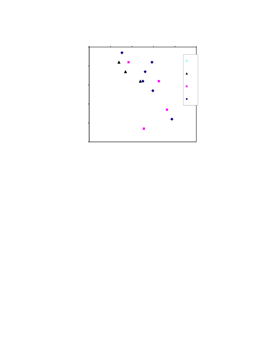
114
0
10
20
30
40
50
0
10
20
30
40
50
Dep
th
(ft)
Moisture Content (%)
UH 1
UH 2
UH 3
UH 4
Fig. 4.9. Variation of Moisture Content with Depth at NASA Rd. 1.
Liquid Limit and Plastic Limit Tests
Liquid limit and plastic limit tests were conducted on eight soil samples. Since the
top 20 ft of the soil was embankment, tests were conducted on samples below the
embankment. Both liquid limit and plastic limit were relatively high around the 23 ft
depth. The liquid limit was in the range of 60% and 70% while the plastic limit was in the
range of 15% and 25% as shown in Fig. 4.10.
As the depth increased, the liquid limit decreased to 34% (except for one datum
point (Fig. 4.10)) and the plastic limit to 7%. Data in the TxDOT report on NASA Rd. 1
indicted that the liquid limit varied from 56 to 80% and it increased with depth. Still, the
LL at NASA Rd.1 was within the range of LL measured at the SH3 site.
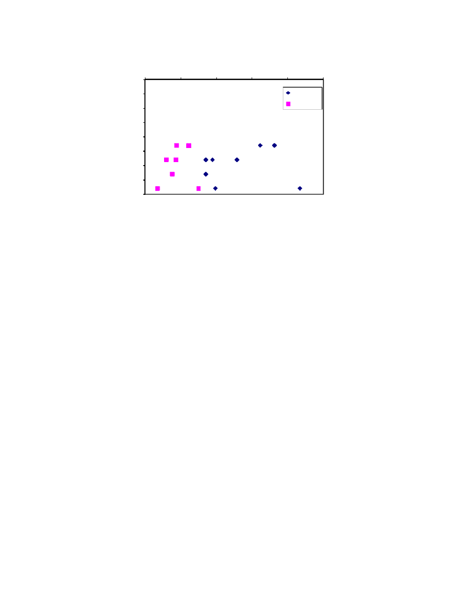
115
0
5
10
15
20
25
30
35
40
0
20
40
60
80
100
Atterberg Limits (%)
Liquid limit
Plastic limit
Fig. 4.10. Liquid Limit and Plastic Limit of the Soils along the Depth.
Unconfined Compressive Strength Tests
Nine strength tests were conducted on the soil samples collected. The depth of the
samples ranged from 18 ft to 40 ft. The shear strength of the soil ranged between 3 psi
and 6 psi up to the 38 ft depth (Fig 4.11). Much higher soil strength was observed near
the 39 ft depth and it was 14.5 psi. The shear strength at the SH3 site varied from 2 psi to
18 psi. So the soil at the SH3 site had comparable strength to the NASA Rd.1 site.
Incremental Load (IL) Consolidation Tests
Seven traditional consolidation tests were conducted on the samples collected
from the depths between 20 and 40 ft below the ground surface. For all the consolidation
tests, pre-consolidation pressure, compression index, and three recompression indices
were obtained. The parameters obtained from consolidation tests are summarized in
Table 4-5.
Dept
h (
ft)
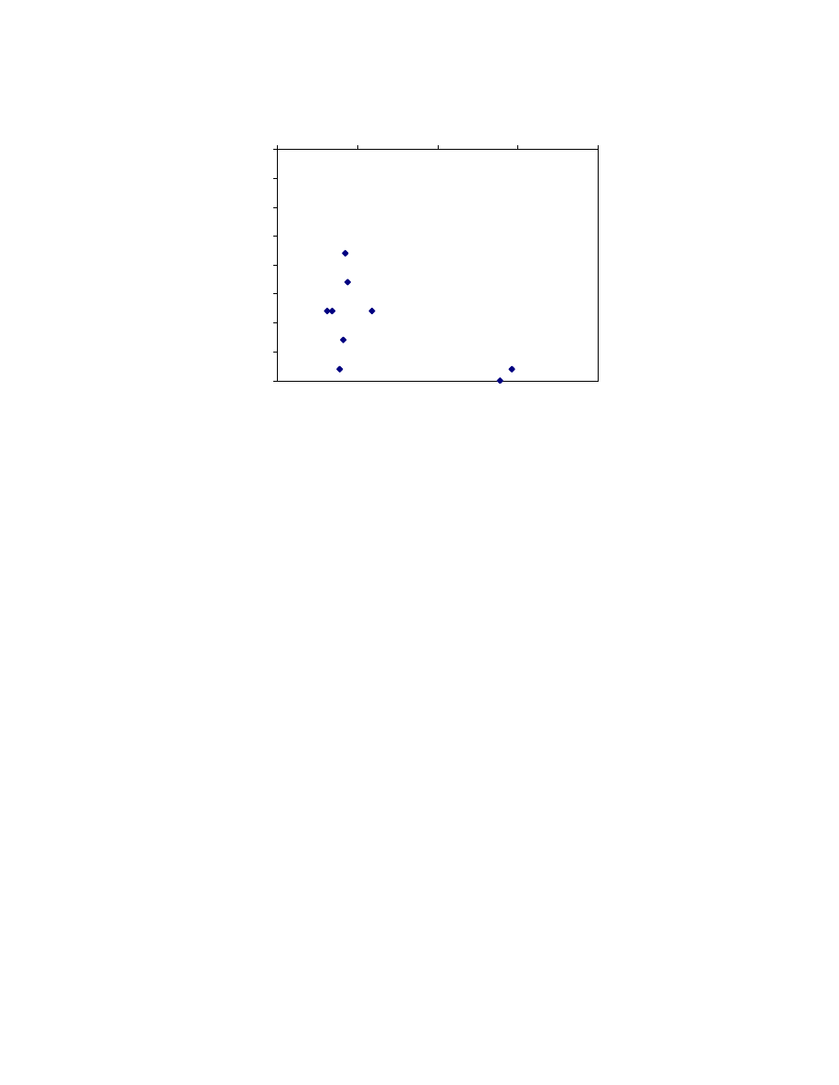
116
0
5
10
15
20
25
30
35
40
0
5
10
15
20
Shear Strength Su (psi)
D
ept
h (
ft
)
Fig. 4.11. Shear Strength Variation with Depth at NASA Rd. 1.
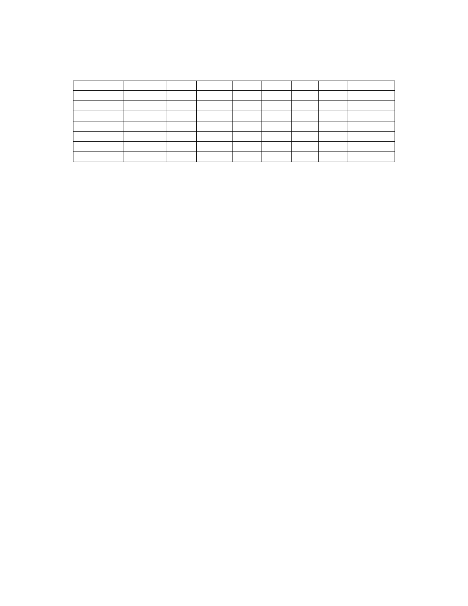
117
Table 4-5. Consolidation Parameters from IL Consolidation Tests for NASA Rd. 1.
In Fig. 4.12, the C
c
and C
r
values obtained during this study are compared with
data from earlier investigations performed in 1994 and 2005. As seen in Fig. 4.12, the
compression index values compare well with the new data. The recompression index
values (C
r2
) were also in good agreement except for the two data points from the 2005
consolidation tests. These two recompression indices were comparable to the C
r1
from the
current study.
Sample Depth
(ft) e
0
σ
p
(psf)
C
c
C
r1
C
r2
C
r3
Comment
UH-1 27-29
28 1.065 2144 0.546
0.069 0.119 0.127
Soft
*
UH-1 37-39
38 0.830 2406 0.173
0.030 0.076 0.081
Soft
**
UH-2 22-24
23 0.972 2094 0.375
0.019 0.079 0.077 Very
Soft
**
UH-3 22-24
23 0.736 3820 0.333
0.037 0.067 0.070 Very
Soft
**
UH-3 27-29
28 0.900 2352 0.296
0.028 0.041 0.047
Soft
*
UH-3 32-34
33 0.735 3820 0.284 --- 0.040
0.044 Very
Soft
**
UH-3 37-39
38 1.041 3032 0.298
0.028 0.047 0.052 Very
Soft
**
*
Based on the unconfined compressive strength test results for S
u
≤ 3.63 psi
(Terzaghi and Peck 1967)
**
Based on the TCP values (TxDOT Geotechnical Manual 2006)
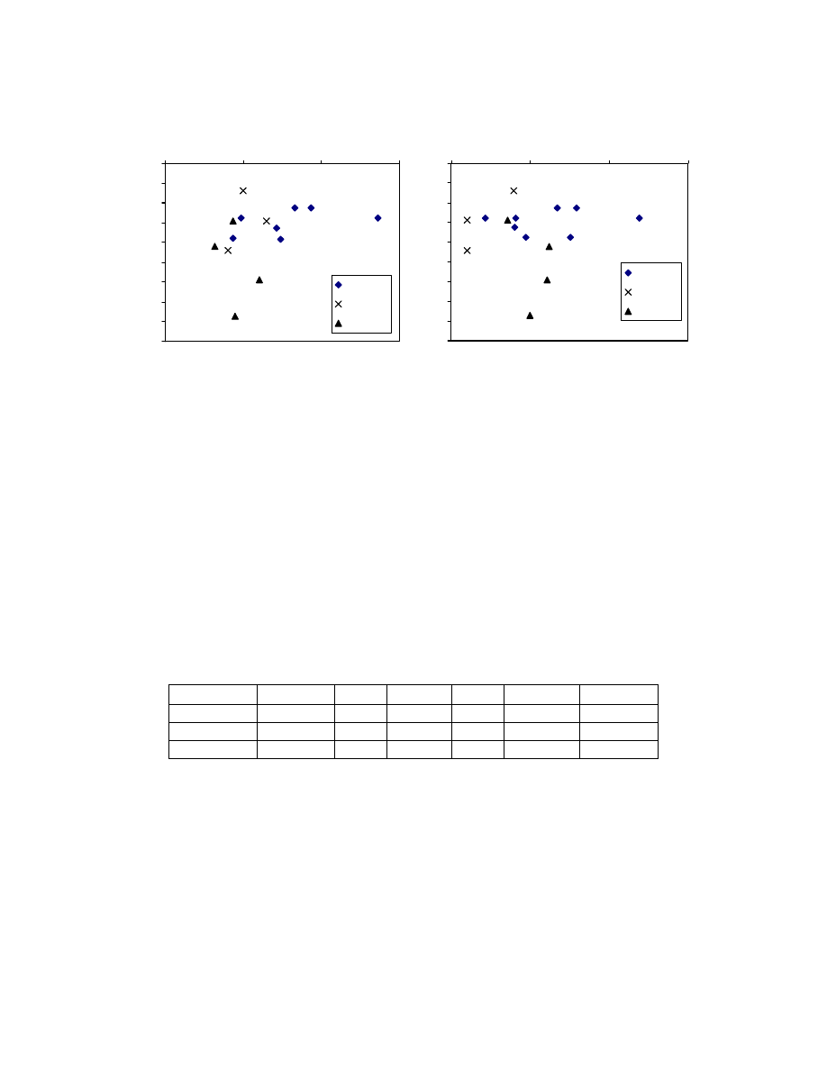
118
(a) C
c
(b)
C
r2
Fig. 4.12. Variation of New and Old (a) C
c
and (b) C
r2
with Depth.
Incremental Load Consolidation Test with Multiple Unloading–Reloading
To investigate the effect of the unloading stress level on the recompression index,
three consolidation tests were conducted with multiple unloading–reloading cycles.
General properties of the soil samples are given in Table 4.6. Two of the soil samples
were high plasticity clay, CH, while one of them was low plasticity clay, CL.
Table 4-6. Soil Parameters of the Samples Used for Consolidation Tests with
Multiple Loops.
Sample Depth
(ft) e
0
LL
(%) PI Soil
Type
Comment
UH-2 22-24
23 1.057 72.67 55.02 CH Very
Soft
*
UH-2 27-29
28 0.682 34.10 16.85 CL Very
Soft
*
UH-3 22-24
23 0.736 64.65 40.16 CH Very
Soft
*
*
Based on the TCP values (TxDOT Geotechnical Manual 2006)
Typical vertical effective stress versus void ratio relationships for a soil sample
(UH-2-22-24) is shown in Fig. 4.13. Similarly the consolidation tests for UH-3 22-24 had
four loops, while soil sample UH-2 27-29 had six loops. It can be observed that the slope
of the unloading–reloading curves increased while vertical effective stress was increased.
0
10
20
30
40
50
60
70
80
90
0
0.2
0.4
0.6
Compression Index (Cc)
D
epth
(ft)
UH-2007
AT-2005
TB-1994
0
10
20
30
40
50
60
70
80
90
0
0.05
0.1
0.15
Recompression Index (Cr)
D
ep
th (ft)
UH-2007
AT-2005
TB-1994
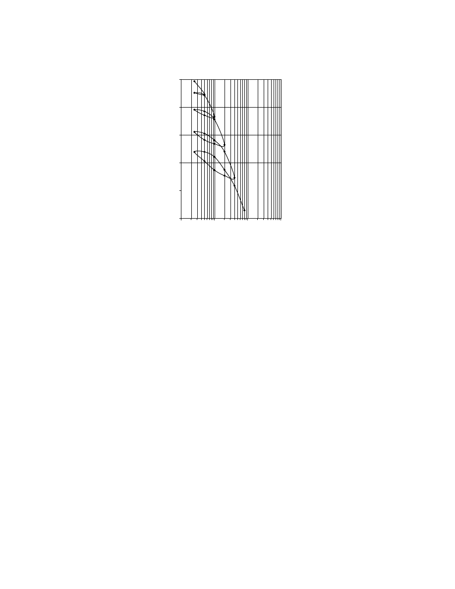
119
0.80
0.85
0.90
0.95
1.00
1.05
0.1
1
10
100
()
Fig. 4.13.Void Ratio versus Vertical Effective Stress Relationship for CH Soil
(Sample UH-2 22-24) with Multiple Loops.
4.3. Soil
Characterization
- The data from SH3 and NASA Rd. 1 are compared to the other published
data in the literature (Vipulanandan et al. 2007) on deltaic clays using the
Casagrande plasticity chart (Fig. 4.14). The results are comparable and
within the A and U-lines on the plasticity chart.
Void
R
ati
o e
Vertical effective stress (tsf)
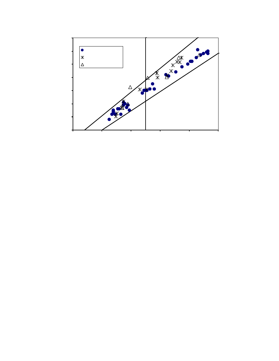
120
0
10
20
30
40
50
60
70
0
20
40
60
80
100
Liquid Limit (%)
P
las
ti
ci
ty I
nd
ex
(%
)
Houston - Galveston
SH3
NASA RD 1
Fig. 4.14. Comparing the SH3 and NASA Rd.1 Data on Casagrande Plasticity
Chart.
4.4.
Preconsolidation Pressure (
σ
p
)
The preconsolidation pressure of a clay soil is defined as the highest stress the clay
soil ever felt in its history. It is also defined as the yield stress of the soil. Several
methods were developed to determine the preconsolidation pressure,
σ
p
, and they are as
follows (Şenol
and Sağlamer 2000):
1. Casagrande method (e - log
σ’)
2. Schmertmann method (e - log
σ’)
3. Janbu methods (
Δ
H/H -
σ’ and M
c
-
σ’)
4. Butterfield method (ln(1 + e) – log P’)
5. Tavenas method (
Δ
H/H -
σ’)
6. Old method (
Δ
H/H – log
σ’)
7. Van Zelst method (
Δ
H/H – log
σ’).
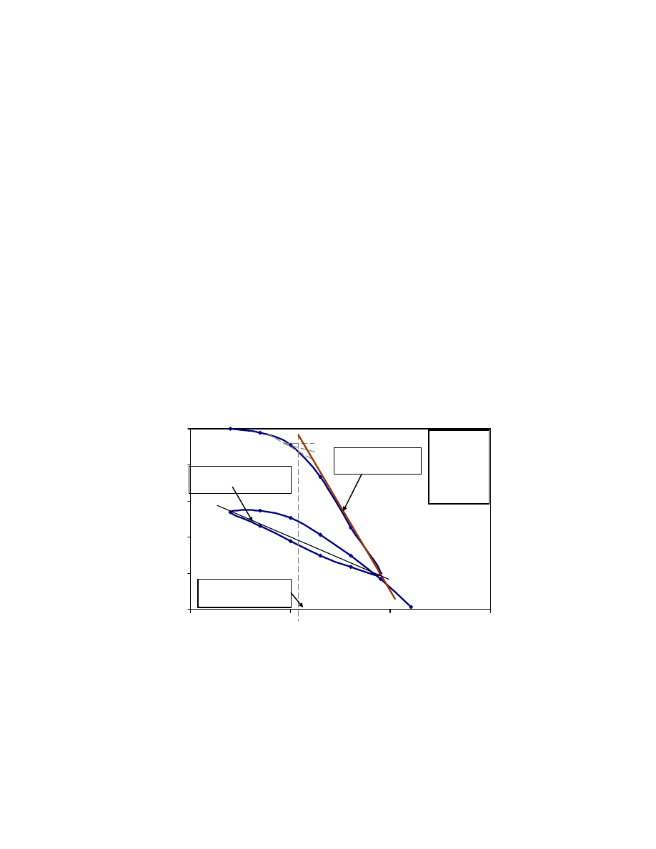
121
They are classified into two main groups:
- the direct determination methods: Janbu and Tavenas methods (Fig. 4.16)
- the graphical methods: the five remaining methods (Figs. 4.15 and 4.17.).
The Casagrande graphical method (e - log
σ’) is the most widely used and the one
used by TxDOT (Fig. 4.15).
Data obtained from the standard incremental load consolidation performed on a
clay sample obtained from SH3 Borehole B1 at a depth of 18-20 ft were used to
determine the preconsolidation pressure using the different existing methods. It was a
high plasticity clay with LL = 73.5% and PI = 51.5% and classified as CH clay according
to the USCS system.
0.60
0.70
0.80
0.90
1.00
1.10
0.1
1.0
10.0
100.0
Vertical applied stress at log scale
σ
v
(tsf)
Vo
id
Ra
ti
o
e
e
o
= 1.10
σ'
0
= 0.78tsf
σ
p
= 1.36 tsf
C
c
= 0.443
Cr =0.114
1
5
3
2
6
4
σ
p
:
t he
prec o ns o lida tio n pre s s ure
S lo pe o f this line is
C
c
the c o m pre s s io n inde x
S lo pe o f this line is C
r
the
re co m pres s io n index
Fig. 4.15. e – log
σ’ Curve Showing Casagrande Graphical Method (Method 1) for
σ
p
Determination (Clay Sample from SH3 Borehole 1, Depth 18-20 ft, CH Clay).
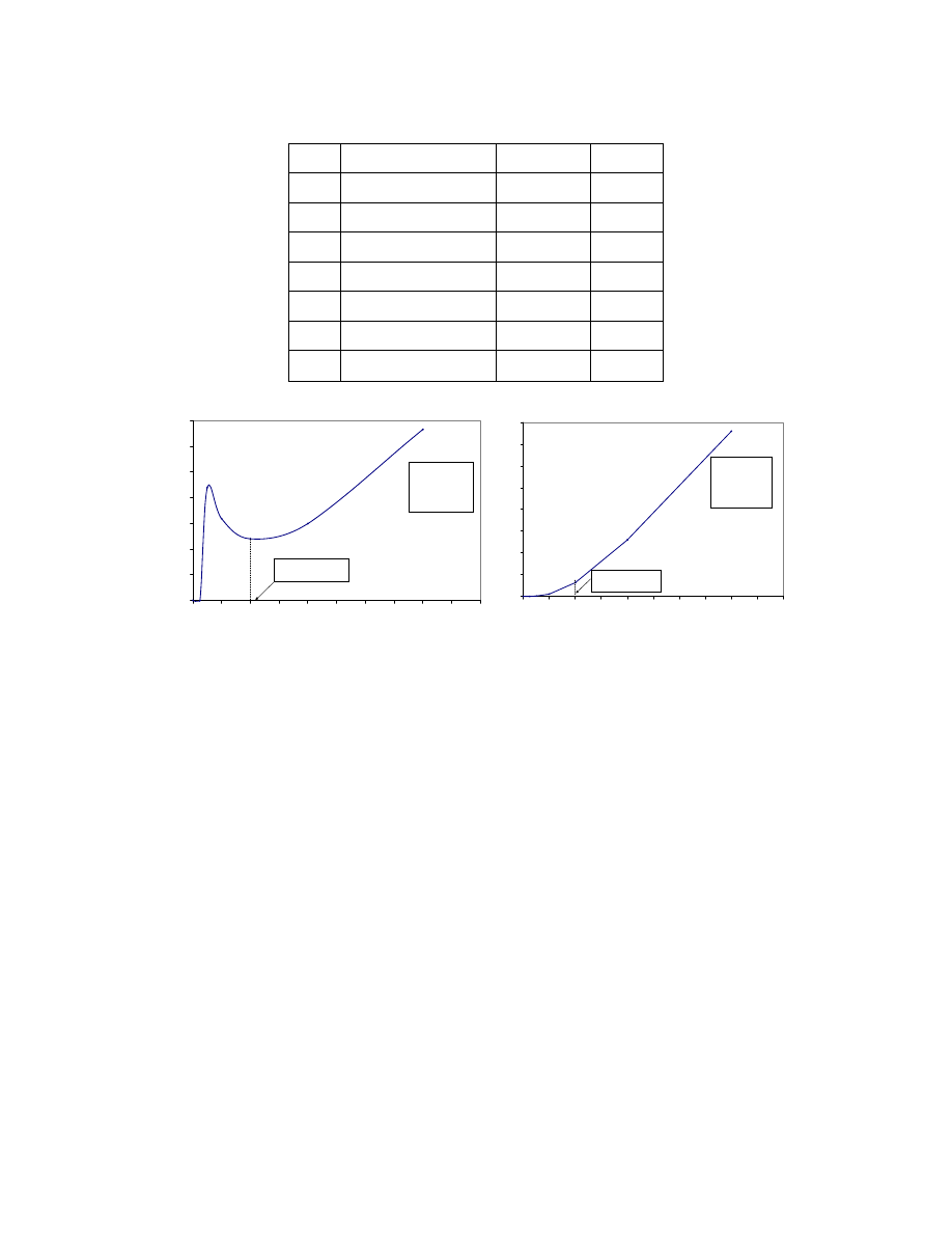
122
Table 4.7. Estimated Preconsolidation Pressure.
No Methods
σ
p
(tsf) OCR
1 Casagrande
1.36 1.74
2 Janbu
2.00 2.56
3 Tavenas
2.00 2.56
4 Schmertmann 1.15 1.47
5 Butterfield
1.40 1.79
6 Old
1.00 1.28
7 Van
Zelst
1.76 2.26
0
10
20
30
40
50
60
70
0
1
2
3
4
5
6
7
8
9
10
Vertical effective stress σ' (tsf)
dσ
'/
d
ε
(ts
f)
e
o
= 1.10
σ
p
= 2 tsf
C
c
= 0.443
σ
p
: the preconsolidation
pressure
0.00
0.20
0.40
0.60
0.80
1.00
1.20
1.40
1.60
0
1
2
3
4
5
6
7
8
9
10
Vertical applied stress
σ'
(tsf)
σ
'
d
ε
(t
sf)
σ
p
:
the preconsolidation
pressure
e
o
= 1.10
σ
p
= 2 tsf
C
c
= 0.443
Janbu method
Tavenas method
Fig. 4.16. Direct Determination Methods for Preconsolidation Pressure.
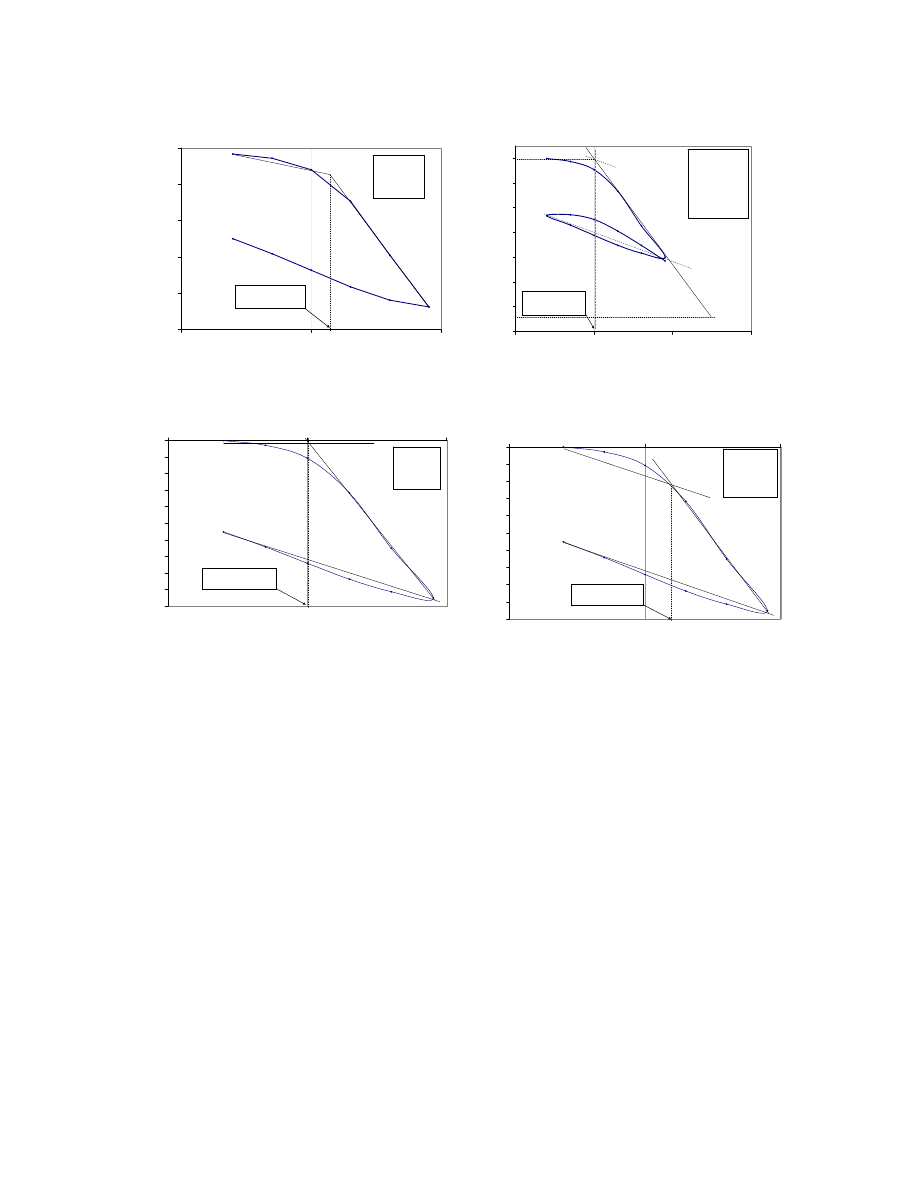
123
0.50
0.55
0.60
0.65
0.70
0.75
0.1
1.0
10.0
Vertical effective stress
σ'
(tsf)
ln
(1
+
e)
e
o
= 1.10
σ
p
= 1.4 tsf
Cc = 0.443
σ
p
:
the preconsolidation
pressure
0.40
0.50
0.60
0.70
0.80
0.90
1.00
1.10
0.1
1.0
10.0
100.0
Vertical effective stress
σ' (tsf)
Vo
id
Ra
ti
o
e
e
o
= 1.10
σ
p
= 1.15tsf
C
c
= 0.443
σ
p
:
the preconsolidation
pressure
σ
o
=1.15 tsf
Butterfield method
Schmertmann method
0
2
4
6
8
10
12
14
16
18
20
0.1
1.0
10.0
Vertical effective stress
σ
' (tsf)
St
rai
n
ε
(%
)
e
o
= 1.10
σ
p
= 1. sf
C
c
= 0.443
σ
p
:
the preconsolidation
pressure
0
2
4
6
8
10
12
14
16
18
20
0.1
1.0
10.0
Vertical effective stress
σ'
(tsf)
St
rain
ε
(%
)
e
o
= 1.10
σ
p
= 1.76 tsf
C
c
= 0.443
σ
p
: the preconsolidation
pressure
Old method
Van Zelst method
Fig. 4.17. Graphical Methods of Determining the Preconsolidation Pressure.
The direct determination methods give the highest preconsolidation pressure of
2 tsf; it was noted that their accuracies depended on the load increment, and hence, the
error is higher with higher value of preconsolidation pressure. For the record, the Tavenas
method is the strain energy method.
Using the graphical methods, preconsolidation pressure varied from 1 tsf using
the Old method to 1.76 tsf using the Van Zelst method. The preconsolidation pressure
being the yield stress of the clay soil, and assuming the reliability of the consolidation

124
test, the Casagrande method, which consists of determining the yield point on the
consolidation curve, was a relatively easy method and the results were reproducable. The
remainder of the graphical methods, Schmertmann, Butterfield, Old, and Van Zelst
methods, are all based on approximate linearization of the real consolidation curve. In
particular, the Butterfield method is based on critical state theory. It is useful in cases of
considerable disturbance of the clay soil sample. Consequently, the Casagrande method is
the most widely used and is the one used in this study.
4.5.
Compression Index (C
c
)
The compression index (C
c
) is the slope of the virgin compression part of the
e – log
σ
’ curve and is defined as follows:
1
2
c
log
e
C
σ
σ
Δ
=
4-1
This represents the slope of section 3-4 in Fig. 4.15 and is represented as
3
4
3
4
c
log
)
e
e
(
C
σ
σ
−
−
=
4-2
The compression index (C
c
) for various soils are summarized in Table 4.8. At the
SH3 site, C
c
for the CH clay varies from 0.14 to 0.45, which was in the range of medium
sensitive clay, Chicago clay and Boston Blue clay (Table 4.8). At the NASA Rd.1 site,
the C
c
varied from 0.28 to 0.55, closer to the Boston Blue clay.

125
Table 4.8. Summary Table of Compression Indices for Various Clay Soils (Holtz
and Kovacs 1981).
Deposition
type
C
c
-
0.2 to 0.5
glacial
0.15 to 0.3
marine
0.3 to 0.5
-
0.5 to 0.6
marine
1 to 3
marine
1 to 4
volcanic
7 to 10
-
4 and up
-
10 to 15
-
1.5 to 4.0
-
0.4 to 1.2
-
0.7 to 0.9
marine
0.4
San Francisco Old Bay clays (CH)
Bangkok clay (CH)
Organic clays (OH)
Peats (Pt)
Organic silt and clayey silts (ML-MH)
San Francisco Bay Mud (CL)
Vicksburg Buckshot clay (CH)
Swedish medium sensitive clays (CL-CH)
Canadian Leda clays (MH)
Mexico City clay (MH)
Soil
Normally consolidated medium sensitive clays
Chicago silty clay (CL)
Boston blue clay (CH)
4.5.1. Compression index correlation
Several correlations have been developed to determine the compression index
from the natural moisture content (W
n
) or liquid limit (LL) for some specific clay soils
(Table 4.9).
Ganstine (1971) proposed several linear correlations for the Beaumont clay in the
Houston area. Based on the data collected by Ganstine (1971) and using the data from the
current study, it is being proposed to relate the C
c
to the moisture content and unit weight
of the soil (Fig. 4.18 and Fig. 4.19).
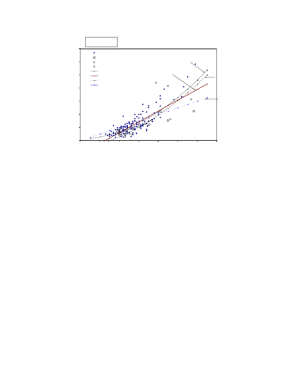
126
0.0
0.2
0.4
0.6
0.8
1.0
1.2
1.4
0
10
20
30
40
50
60
70
Moisture content (%)
C
om
pr
esssi
on
in
de
x
Ganstine (1971)
SH3 (2007)
SH 146 (2006)
Riverside (2006)
Polynomial fit
Linear fit
Chicago clay polyno. fit
Chicago clay linear fit
193 data points
Chicago
Clay soil
Linear fit
(Houston)
Polynomial fit
(Houston)
Chicago
Clay soil
Fig. 4.18. Correlation of Compression Index of Houston/Beaumont Clay Soil with
In-situ Moisture Content.
One hundred ninety-three compression indices of the Houston clay, obtained from
the standard incremental load consolidation test, were used to develop the correlations.
• C
c
versus moisture content
The second order polynomial relationship is as follows:
2
n
3
2
n
4
c
10
.
756
.
1
W
10
.
297
.
1
W
10
.
298
.
2
C
−
−
−
+
+
=
4-3
with a coefficient of correlation (R) = 0.83.
The linear relationship is as follows:
2108
.
0
W
10
.
65
.
1
C
n
2
c
−
=
−
4-4
with R = 0.81.
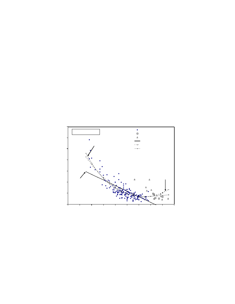
127
Based on Fig. 4.18, it is recommended using the linear fitting correlation equation
for natural moisture content within the range of 20% and 40% for a good estimation of
the recompression index. The second order polynomial relationship is the better one and
can be used for any value of in-situ moisture content. These correlations were established
independently of the type of clay (CL or CH) and are quite useful for estimating the
compression index, knowing only the in-situ moisture content and without performing
any consolidation or even an Atterberg’s limit tests.
Houston clay soil has higher compressibility compared to Chicago clay soils
(Fig. 4.18). Chicago clay soil correlations are summarized in Table 4.9.
0.0
0.2
0.4
0.6
0.8
1.0
1.2
1.4
50
60
70
80
90
100
110
120
130
140
C
om
pr
es
ss
io
n in
de
x
Ganstine (1971)
SH146 (2006)
SH3 (2007)
linear fit
2nd order polynomial fit
3rd order polynomial fit
180 data points
Linear fit
Third order
polynomial fit
Second order
polynomial fit
Unit weight (pcf)
Fig. 4.19. Correlation of Compression Index of Houston/Beaumont Clay Soil with
In-situ Unit Weight.

128
• C
c
Versus Unit weight of Soils
The linear relationship is as follows:
245
.
1
W
10
.
01
.
1
C
n
2
c
+
−
=
−
4-5
with R
= 0.7
The second order polynomial relationship is as follows:
0458
.
4
10
.
87
.
6
10
.
3
C
2
2
4
c
+
−
=
−
−
γ
γ
4-6
with R
= 0.8.
The third order polynomial relationship is as follows:
0264
.
7
1626
.
0
10
.
3
.
1
10
.
3
C
2
3
3
6
c
+
−
+
−
=
−
−
γ
γ
γ
4-7
with R
= 0.81.
Based on prediction error, it is recommended to use the linear relationship to
estimate the C
c
when the unit weight is in the range of 80 and 110 pcf. The second order
polynomial relationship is as good as the third order up to a unit weight of 120 pcf. Over
120 pcf, it is better to use the third order polynomial relationship for estimating the
recompression index.

129
Table 4.9. Correlations for C
c
(Azzouz et al. (1976); Holtz and Kovacs (1981)).
Regions of Applicability
C
c
=
Remolded clays
C
c
=
Chicago clays
C
c
=
Chicago clays
C
c
=
All clays
C
c
=
Inorganic, cohesive soil; silt, some clay;
silty clay;clay
C
c
=
Organic soils-meadow mats, peats, and
organic silt and clay
C
c
=
Soils of very low plasticity
C
c
=
All clays
C
c
=
Chicago clays
1.15(e
o
- 0.35)
0.3(e
o
- 0.27)
1.15x10
-2
w
n
0.75(e
o
- 0.50)
Equations
17.66x10
-5
w
n
2
+ 5.93x10
-3
w
n
- 0.135
0.007(LL - 7)
0.208e
o
+ 0.0083
0.156e
o
+ 0.0107
0.01w
n
4.5.2. Stress dependency of incremental compression index (C’
c
)
The stress dependency of the compression index was mentioned by Leroueil et al.
(1990), in which a representative value of the field condition is to be chosen for
settlement calculation and that the current practice usually takes the slope of the secant
drawn across the experimental curve from
vi
'
0
v
'
p
to
σ
Δ
σ
σ
+
(Fig. 4.15). In this study,
incremental load consolidation test results from SH3 samples were used for more detail
analyses. The incremental compression index (de/d(logσ) was determined from the
primary consolidation relationships. From laboratory consolidation tests on the Houston
clay soil, it was noticed that the recompression index, in fact, is stress dependent as can
be seen in Fig. 4.20(a, b, c, d, e, f, g, and h). The C
c
was stress dependent and this
observation was true for both CL and CH clays.
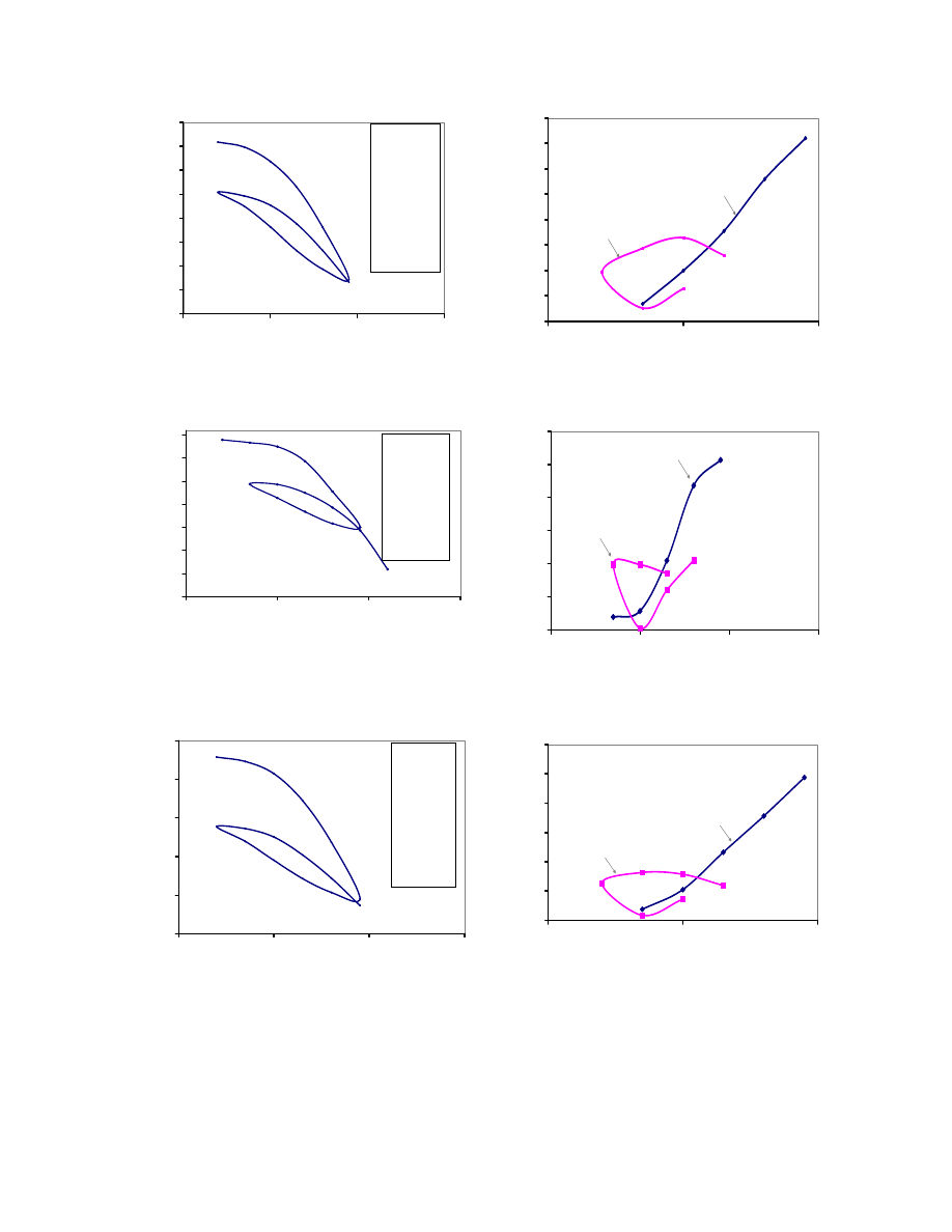
130
0.42
0.44
0.46
0.48
0.50
0.52
0.54
0.56
0.58
0.1
1.0
10.0
100.0
Vertical effective stress
σ'
(tsf)
Vo
id
r
at
io
e
e
o
= 0.55
σ
p
= 1.86 tsf
C
c
= 0.144
C
r1
= 0.018
C
r2
= 0.049
C
r3
= 0.062
C
r1
/C
c
= 0.125
Cr
2
/C
c
= 0.340
Cr
3
/C
c
= 0.431
LL = 58.2 %
PL = 18.3 %
0.00
0.02
0.04
0.06
0.08
0.10
0.12
0.14
0.16
0
1
10
Vertical effective stress σ' (tsf)
C'
&
C
r
C
r
C'
a) SH3 B1_2 – 4 ft (CH)
0.50
0.55
0.60
0.65
0.70
0.75
0.80
0.85
0.1
1.0
10.0
100.0
Vertical effective stress
σ
' (tsf)
Vo
id
r
at
io
e
e
o
= 0.84
σ
p
= 1.91 tsf
C
c
= 0.257
C
r1
= 0.032
C
r2
= 0.081
C
r3
= 0.099
C
r1
/C
c
=0.125
C
r2
/C
c
=0.315
C
r3
/C
c
=0.385
LL = 67.5 %
PL = 22.6 %
0.00
0.05
0.10
0.15
0.20
0.25
0.30
0
1
10
100
Vertical effective stress
σ' (tsf)
C'
& C
r
C
r
C'
b) SH3 B1_10 – 12 ft (CH)
0.50
0.55
0.60
0.65
0.70
0.75
0.1
1.0
10.0
100.0
Vertical effective stress
σ'
(tsf)
Vo
id
r
at
io
e
e
o
= 0.73
σ
p
= 1.9 tsf
C
c
= 0.244
C
r1
= 0.022
C
r2
= 0.065
C
r3
= 0.080
C
r1
/C
c
= 0.090
C
r2
/C
c
= 0.266
C
r3
/C
c
= 0.328
LL = 64.8 %
PL = 23.2 %
0.00
0.05
0.10
0.15
0.20
0.25
0.30
0
1
10
Vertical effective stress
σ'
(tsf)
C'
&
C
r
C
r
C'
c) SH3 B1_12 – 14 ft (CH)
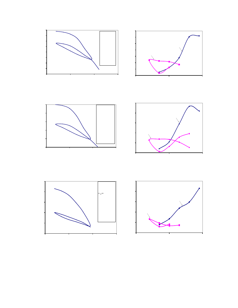
131
0.45
0.50
0.55
0.60
0.65
0.70
0.75
0.80
0.85
0.1
1.0
10.0
100.0
Vertical effective stress
σ'
(tsf)
Vo
id
r
at
io
e
e
o
= 0.86
σ
p
= 2 tsf
C
c
= 0.306
C
r1
= 0.0414
C
r2
= 0.099
C
r3
= 0.111
C
r1
/C
c
= 0.135
C
r2
/Cc = 0.324
C
r3
/Cc = 0.363
LL = 75 %
PL = 19.8 %
0.00
0.05
0.10
0.15
0.20
0.25
0.30
0.35
0
1
10
Vertical effective stress
σ
'
(tsf)
C'
&
C
r
C
r
C'
d) SH3 B1_14 – 16 ft (CH)
0.60
0.70
0.80
0.90
1.00
1.10
0.1
1.0
10.0
100.0
Vertical applied stress
σ
v
(tsf)
Vo
id
r
at
io
e
e
o
= 1.10
Swelling potential:
0.25tsf
σ
p
= 1.36 tsf
C
c
= 0.443
C
r1
= 0.026
C
r2
= 0.117
C
r3
= 0.136
C
r1
/C
c
= 0.059
C
r2
/C
c
= 0.264
C
r3
/C
c
= 0.307
LL = 73.5 %
PL = 22 %
0.00
0.10
0.20
0.30
0.40
0.50
0
1
10
Vertical effective stress
σ
'
(tsf)
C'
&
C
r
C
r
C'
e) SH3 B1_18 – 20 ft (CH)
0.34
0.36
0.38
0.40
0.42
0.44
0.1
1.0
10.0
100.0
Vertical effective stress
σ'
(tsf)
Vo
id
r
at
io
e
e
o
= 0.43
σ
p
= 1.76 tsf
C
c
= 0.086
C
r1
=
C
r2
= 0.018
C
r3
= 0.016
C
r2
/C
c
= 0.186
C
r3/
C
c
= 0.209
LL = 29.5 %
PL = 19.1 %
0.00
0.02
0.04
0.06
0.08
0.10
0
1
10
Vertical effective stress
σ
'(tsf)
C'
&
C
r
C
r
C'
f) SH3 B1_22 – 24 ft (CL)
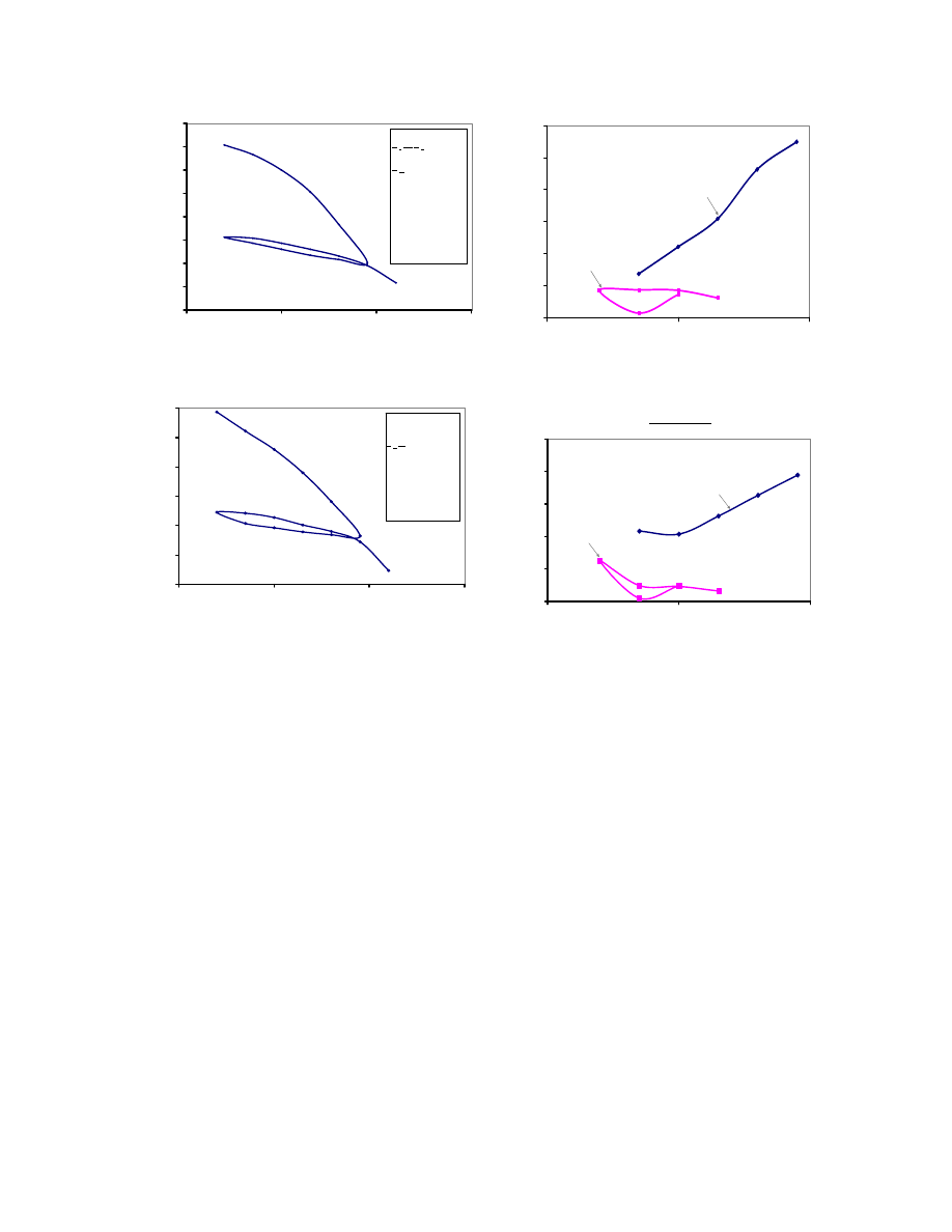
132
0.30
0.32
0.34
0.36
0.38
0.40
0.42
0.44
0.46
0.1
1.0
10.0
100.0
Vertical effective stress
σ'
(tsf)
Voi
d
r
at
io
e
e
o
= 0.47
σ
p
=
σ
o
C
c
= 0.101
C
r1
=
C
r2
= 0.015
C
r3
= 0.017
C
r2
/C
c
= 0.149
C
r2
/C
c
= 0.168
LL = 30.3 %
PL = 17.5 %
0.00
0.02
0.04
0.06
0.08
0.10
0.12
0
1
10
Vertival effective stress
σ'
(tsf)
C'
&
C
r
C
r
C'
g) SH3 B1_24 – 26 ft (CL)
0.27
0.31
0.35
0.39
0.43
0.47
0.51
0.1
1.0
10.0
100.0
Vertical effective stress
σ'
(tsf)
Vo
id
r
at
io
e
e
o
= 0.51
σ
p
=
σ
o
C
c1
= 0.131
C
c1
=
C
r2
= 0.024
C
r3
= 0.017
C
r2
/C
c
= 0.183
C
r3
/C
c
= 0.130
LL = 46.1%
PL = 15.3%
0.00
0.04
0.08
0.12
0.16
0.20
0
1
10
Vertical effective stress
σ'
(tsf)
C'
&
C
r
SH3 B1_10-12ft
C
r
C'
h) SH3 B1_28 – 30 ft (CL)
Fig. 4.20. e – log
σ’ of Different Clay Samples from SH3 at Clear Creek Bridge and
Their Respective Compression and Recompression Index versus log
σ’ Curves.
4.6.
Recompression Index (C
r
)
The recompression index (C
r
) is the compressibility of the clay soil up to the
preconsolidation pressure (
σ
p
), meaning the slope of Section 1-2 in Fig. 4.21 for an
undisturbed sample, but since there is no real undisturbed sample, the unloading and
reloading section of the consolidation curve is used to determine the recompression
index.

133
The interest in the recompression index determination is due to the fact that the
Houston clay is mostly overconsolidated, and the stress increase due to the embankment
and the retaining walls, constructed by TxDOT, is mainly around the preconsolidation
pressures. Consequently, the determination of the recompression is highly critical for
settlement estimation.
The objective of this study is to investigate the different methods used to
determine the recompression index and to quantify its variation for the Houston
overconsolidated clay.
4.6.1. Recompression
indices
There is no clear definition for determining the recompression index. A recent
observation was that the recompression index C
r
can be determined by three different
methods (Fig. 4.21) giving three different values that are named in this study by C
r1,
C
r2
,
and C
r3
(Vipulanandan et al. 2008). This fact needs to be investigated and is due to the
stress dependency of the recompression index during the unloading and reloading process
in a consolidation test (Fig. 4.21).
(1) C
r1
is the slope of the line joining the end of the unloading part (Point 5) and the
intersection of the preconsolidation line and the reloading part of the
recompression curve (Point 6) (Vipulanandan et al. 2008).
(2) C
r2
is the average slope of the hysteretic loop (all the unloading and reloading) as
shown in Fig. 4.21 (Holtz and Kovacs 1981).
(3) C
r3
is the slope of the unloading section of the recompression curve (Das 2006).
Even if the value of the recompression index is very small, the difference in the
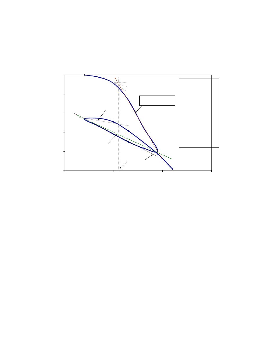
134
values can result in predicting substantially different settlement predictions in
case of overconsolidated soft clay soils (Vipulanandan et al. 2008).
0.60
0.70
0.80
0.90
1.00
1.10
0.1
1.0
10.0
100.0
Vertical effective stress
σ' (tsf)
V
oid ratio e
e
o
= 1.10
Swelling potential: 0.25tsf
σ
p
= 1.36 tsf
C
c
= 0.443
C
r1
= 0.026
C
r2
= 0.117
C
r3
= 0.136
C
r1
/C
c
= 0.056
C
r2
/C
c
= 0.264
C
r3
/C
c
= 0.307
LL = 73.5 %
PL = 22 %
1
5
3
2
6
4
σ
p
Slope of this line is C
c
the compression index
7
C
r1
C
r3
C
r2
Fig. 4.21. e – log
σ’ Curve Showing the Three Recompression Indices (C
r1
, C
r2
, C
r3
).
Clay Sample from SH3 Borehole 1, Depth 18-20 ft, CH Clay.
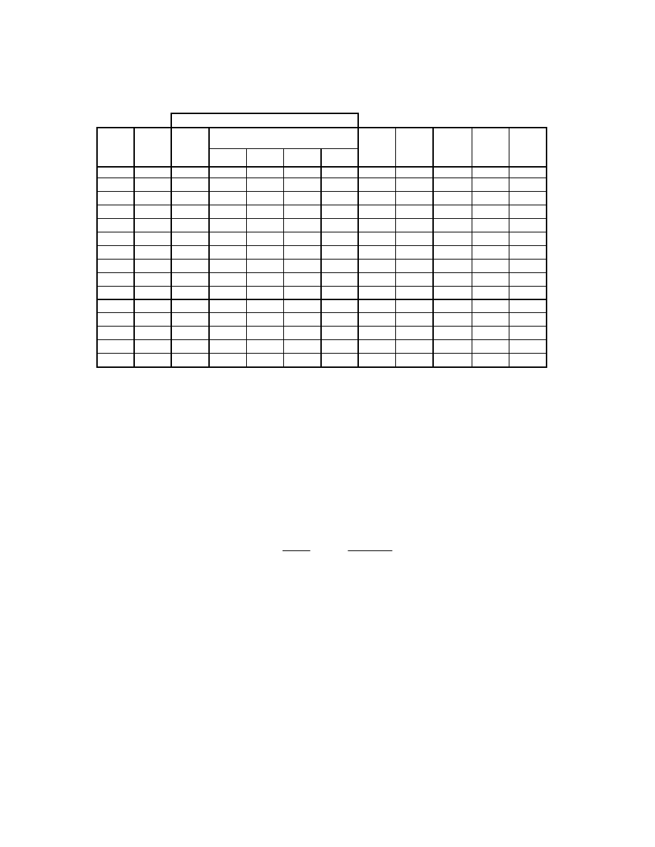
135
Table 4.10. Summary of Compressibility Parameters for the Clay Soils (SH3 Bridge
at Clear Creek).
C
c
C
r1
C
r2
C
r3
1
CH
3
CH
9.6
0.144
0.018
0.049
0.062
3.44
1.27
0.125
0.340
0.431
5
CH
7
CH
9
CH
1.9
0.185
0.018
0.057
0.068
3.78
1.19
0.097
0.308
0.368
11
CH
3.3
0.257
0.032
0.081
0.099
3.09
1.22
0.125
0.315
0.385
13
CH
3.0
0.244
0.022
0.065
0.080
3.64
1.23
0.090
0.266
0.328
15
CH
2.8
0.306
0.041
0.099
0.111
2.71
1.12
0.134
0.324
0.363
17
CH
1.9
0.446
0.025
0.162
0.190
7.60
1.17
0.056
0.363
0.426
19
CH
1.7
0.443
0.026
0.117
0.136
5.23
1.16
0.059
0.264
0.307
21
23
CL
1.1
0.086
0.014
0.018
0.016
1.14
0.89
0.163
0.210
0.187
25
CL
1.0
0.101
-
0.015
0.017
1.13
-
0.149
0.168
27
CL
29
CL
1.0
0.131
-
0.024
0.017
0.71
-
0.183
0.130
C
r3
/C
c
C
r1
/C
c
C
r2
/C
c
Type
C
r3
/C
r1
C
r3
/C
r2
IL TEST
OCR
Compressibility parameters of B1
Depth
(ft)
From Table 4.10, it was observed that for the CH clay soils, C
r3
was equal to 2.71
to 7.60 times the values of C
r1
. This variation will be the same for the magnitude of
settlement estimated using C
r1
and C
r3
, in the case of the overconsolidated clay, when the
total primary settlement S
p
is
⎟⎟
⎠
⎞
⎜⎜
⎝
⎛
Δ
+
+
=
o
o
r
p
H
e
C
S
σ
σ
σ
log
1
0
4-8
Based on the analysis of the data there was no direct correlation between C
r1
and
C’
c
. But there was a linear correlation between C
c
and other recompression indices:
C
r2
= 0.305, C’
c
and C
r3
= 0.356 C’
c
.
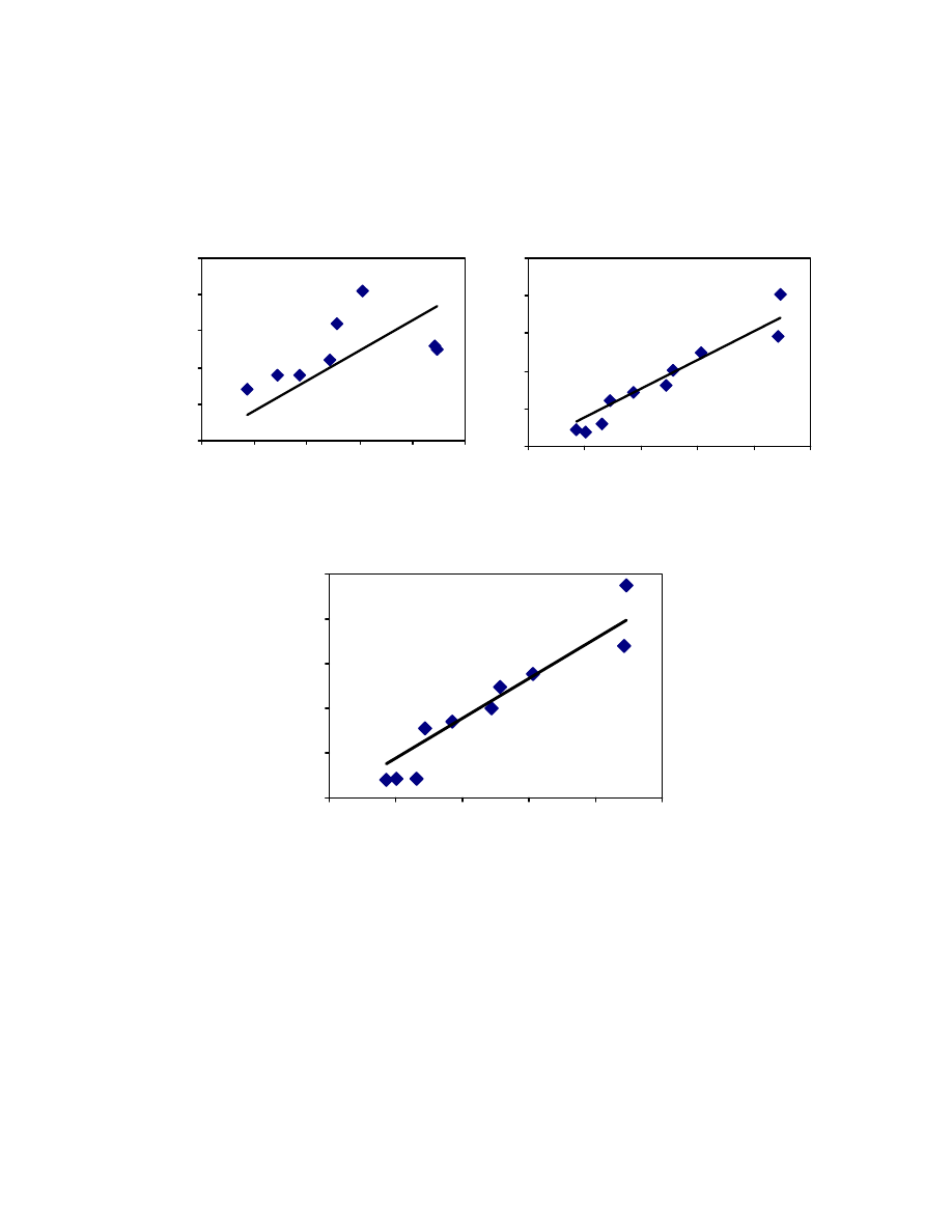
136
As shown on Fig. 4.23, the ratio of recompression indices (C
r2
and C
r3
) and the
compression of the SH3 at Clear Creek clay soil were higher than the New Orleans clay
ratios, except for C
r1
.
a) C
r1
vs C
c
b) C
r2
vs C
c
0.00
0.04
0.08
0.12
0.16
0.20
0.00
0.10
0.20
0.30
0.40
0.50
Cc
C
r3
c) C
r3
vs C
c
Fig. 4.22. Correlation of the Different Types of Recompression Indexes with the
Compression Index a) C
r1
vs. C
c
, b) C
r2
vs. C
c
, and c) C
r3
vs. C
c
.
0.00
0.01
0.02
0.03
0.04
0.05
0.00
0.10
0.20
0.30
0.40
0.50
C
c
C
r1
0.00
0.04
0.08
0.12
0.16
0.20
0.00
0.10
0.20
0.30
0.40
0.50
Cc
C
r2
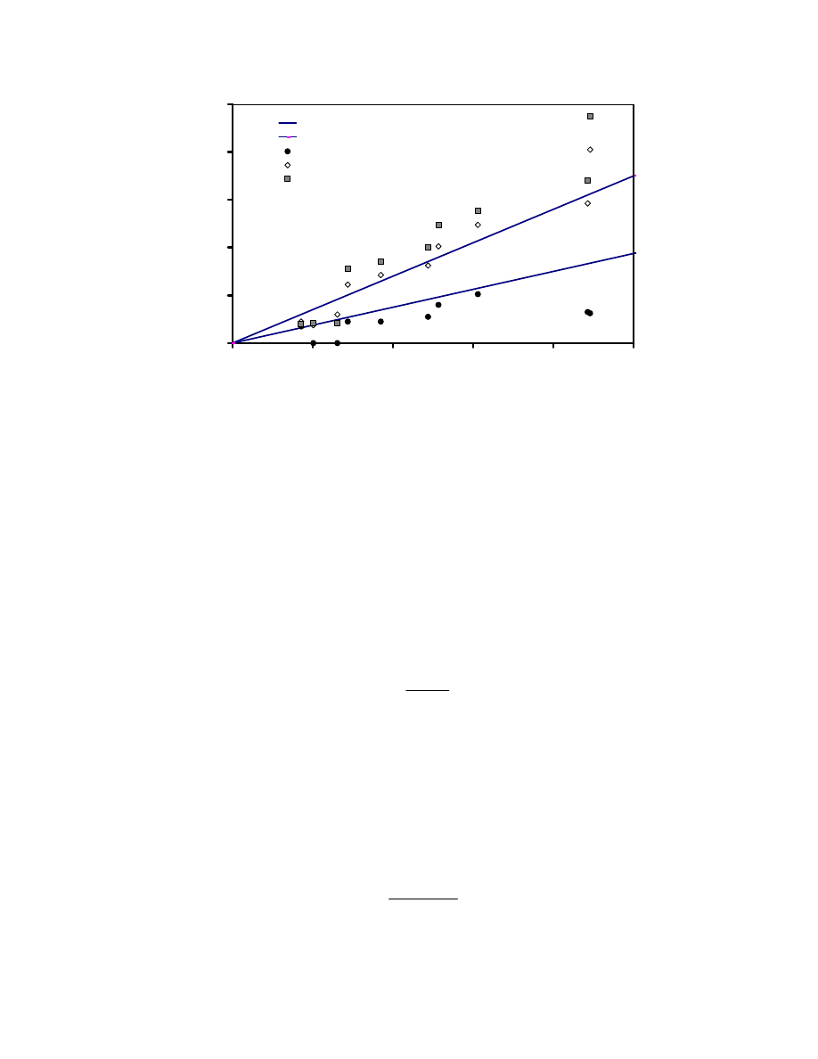
137
0.00
0.04
0.08
0.12
0.16
0.20
0.00
0.10
0.20
0.30
0.40
0.50
Compression index C
c
Recmpression i
ndex
C
r
New Orleans Boundary
New Orleans Boundary
Cr1 (Houston)
Cr2 (Houston)
Cr3 (Houston)
New Orleans clay range
after Das (2004)
Fig. 4.23. Comparison of the Different Recompression Indices of Houston SH3
Samples with New Orleans Clay C
r
/C
c
Range.
4.7.
Coefficient of Consolidation (C
v
)
The coefficient of consolidation derived from Terzaghi’s (1925) 1-D
consolidation theory is the parameter used to determine the percent of the total primary
settlement completed at any time, and is given by the following relationship:
t
H
T
c
2
dr
v
v
=
4-9
where H
dr
is the maximum drainage path.
There are two commonly used methods to calculate the coefficient of
consolidation C
v
:
- Casagrande’s log time method giving
2
50
0.197
dr
v
H
c
t
=
4-10
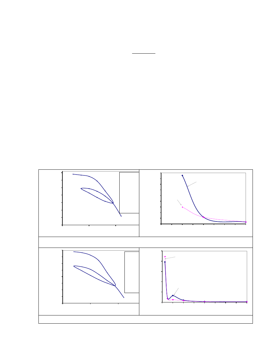
138
- Taylor’s square root of time method giving
2
90
0.848
dr
v
H
c
t
=
4-11
As reported in the literature, Taylor’s square root of time method C
v
values are
generally higher than Casagrande’s logarithm-of-time method values, as was observed in
the current study. For CH clay soils, the coefficient of consolidation was very high before
the preconsolidation pressure and then decreased rapidly thereafter (Fig. 4.24).
In the case of the CL clay soils (silty clay), the coefficient of consolidation
reduced with the stress increase. The Casagrande log-of-time method was not convenient
for the CL soils to the determination of C
v
since the standard shape of the deformation
versus log time was not obtained (Fig. 4.25).
0.50
0.55
0.60
0.65
0.70
0.75
0.80
0.85
0.1
1.0
10.0
Vertical effective stress
σ
' (tsf)
Vo
id ra
tio
e
e
o
= 0.84
σ
p
= 1.91 tsf
C
c
= 0.257
C
r1
= 0.032
C
r2
= 0.081
C
r3
= 0.099
C
r1
/C
c
=0.125
C
r2
/C
c
=0.315
C
r3
/C
c
=0.385
LL = 67.5 %
PL = 22.6 %
0
10
20
30
40
50
60
70
80
90
0.0
0.5
1.0
1.5
2.0
2.5
3.0
3.5
4.0
Vertical effective stress
σ' (tsf)
C
v
(ft
2
/y
r)
Taylor method
Casagrande method
a) SH3 B1 10 – 12 ft (CH)
0.45
0.50
0.55
0.60
0.65
0.70
0.75
0.80
0.85
0.1
1.0
10.0
Vertical effective stress
σ'
(tsf)
Vo
id
r
at
io
e
e
o
= 0.86
σ
p
= 2 tsf
C
c
= 0.306
C
r1
= 0.0414
C
r2
= 0.099
C
r3
= 0.111
C
r1
/C
c
= 0.13
C
r2
/Cc = 0.32
C
r3
/Cc = 0.36
LL = 75 %
PL = 19.8 %
0
50
100
150
200
250
0
1
2
3
4
5
6
7
8
Vertical effective stress
σ' (tsf)
C
v
(f
t
2
/y
r)
Taylor method
Casagrande method
b)
SH3 B1 14 – 16 ft (CH)
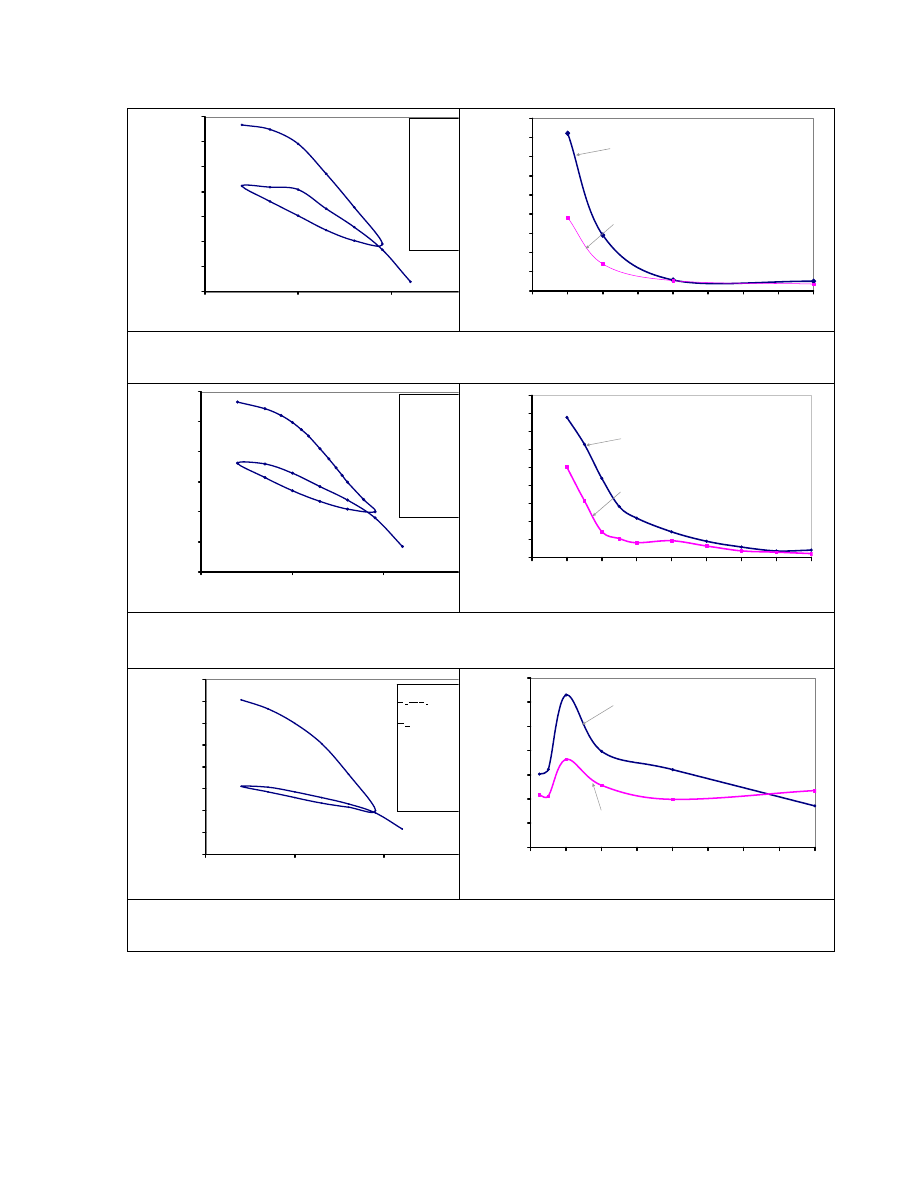
139
0.50
0.60
0.70
0.80
0.90
1.00
1.10
1.20
0.1
1.0
10.0
Vertical effective stress σ' (tsf)
Voi
d
ra
ti
o
e
e
o
= 1.22
σ
p
= 1 tsf
C
c
= 0.446
C
r1
= 0.025
C
r2
= 0.162
C
r3
= 0.190
C
r1
/C
c
= 0.05
C
r2
/C
c
= 0.36
C
r3
/C
c
= 0.42
LL = 73.5 %
PL = 22%
0
10
20
30
40
50
60
70
80
90
0.0
0.5
1.0
1.5
2.0
2.5
3.0
3.5
4.0
Vertical effective stress
σ' (tsf)
C
v
(f
t
2
/y
r)
Taylor method
Casagrande method
c) SH3 B2 16 – 18 ft (CH)
0.40
0.50
0.60
0.70
0.80
0.90
1.00
0.1
1.0
10.0
Vertical effective stress σ' (tsf)
Voi
d
ra
ti
o
e
e
o
= 0.97
σ
p
= 1.2 tsf
C
c
= 0.347
C
r1
= 0.057
C
r2
= 0.169
C
r3
= 0.153
C
r1
/C
c
= 0.164
C
r2
/C
c
= 0.487
C
r3
/C
c
= 0.441
0
2
4
6
8
10
12
14
16
18
0.0
0.5
1.0
1.5
2.0
2.5
3.0
3.5
4.0
Vertical effective stress σ' (tsf)
C
v
(f
t
2
/y
r)
Taylor method
Casagrande method
d) SH3 B2 18 – 20 ft (CH)
0.30
0.32
0.34
0.36
0.38
0.40
0.42
0.44
0.46
0.1
1.0
10.0
Vertical effective stress
σ'
(tsf)
Voi
d
r
ati
o
e
e
o
= 0.47
σ
p
=
σ
o
C
c
= 0.101
C
r1
=
C
r2
= 0.015
C
r3
= 0.017
C
r2
/C
c
= 0.149
C
r2
/C
c
= 0.168
LL = 30.3 %
PL = 17.5 %
0
20
40
60
80
100
120
140
0
1
2
3
4
5
6
7
8
Vertical effective stress
σ'
(tsf)
C
v
(f
t
2
/y
r)
Taylor method
Casagrande method
e) SH3 B1 24 – 26 ft (CL)
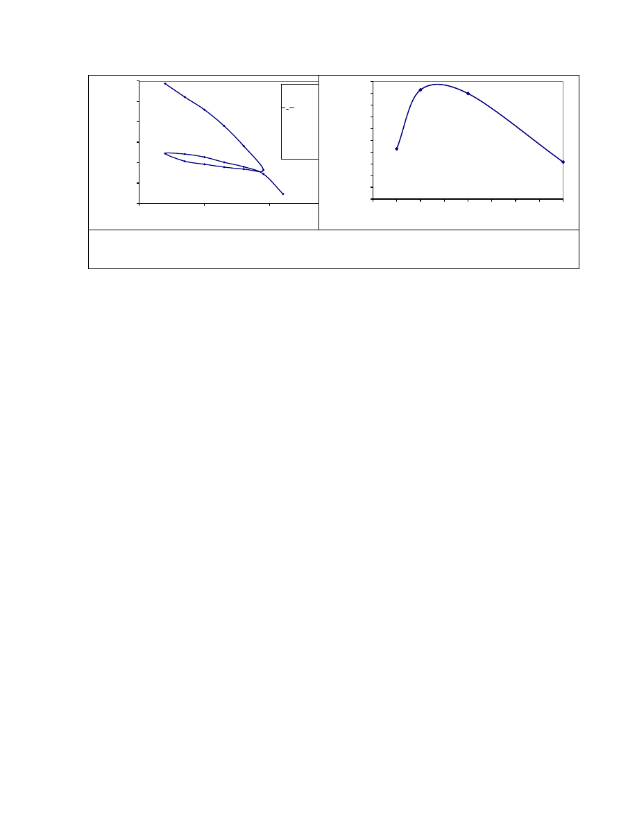
140
0.27
0.31
0.35
0.39
0.43
0.47
0.51
0.1
1.0
10.0
Vertical effective stress
σ'
(tsf)
Vo
id
r
at
io
e
e
o
= 0.51
σ
p
=
σ
o
C
c1
= 0.131
C
c1
=
C
r2
= 0.024
C
r3
= 0.017
C
r2
/C
c
= 0.183
C
r3
/C
c
= 0.130
LL = 46.1%
PL = 15.3%
0
20
40
60
80
100
120
140
160
180
200
0.0
0.5
1.0
1.5
2.0
2.5
3.0
3.5
4.0
Vertical effective stress
σ' (tsf)
C
v
(f
t
2
/y
r)
f) SH3 B1 28 – 30 ft (CL)
Fig. 4.24. e – log
σ’ Curve of a Houston Clay from SH3 and Their Respective C
v
–
σ’
Curve.
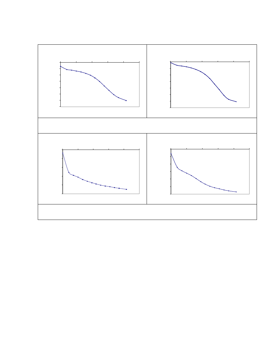
141
2 tsf_SH3 B1_16-18ft
0.05
0.06
0.07
0.08
0.09
0.10
0.11
0.12
0.1
1
10
100
1000
10000
Time (min)
Deform
at
ion
(in)
4 tsf_SH3 B1_16-18ft
0.11
0.12
0.13
0.14
0.15
0.16
0.17
0.18
0.1
1
10
100
1000
10000
Time (min)
D
efor
m
at
ion
(in
)
a) Casagrande method with CH clay
2 tsf_SH3 B1_28-30ft
0.035
0.040
0.045
0.050
0.055
0.060
0.1
1
10
100
1000
10000
Time (min)
Defor
m
ation
(in
)
4 tsf_SH3 B1_28-30 ft
0.055
0.060
0.065
0.070
0.075
0.080
0.085
0.1
1
10
100
1000
10000
Time (min)
Defo
rm
at
ion
(i
n)
b) Casagrande method with CL clay
Fig. 4.25. Deformation vs. Time at log Scale Curve of Casagrande T
50
(a) CH Clay
and (b) CL Clay.
4.8.
Constant Rate of Strain (CRS) Test (ASTM D 4186-86)
The Constant Rate of Strain (CRS) consolidation test is a faster test to determine
the consolidation properties of clay soils than the standard incremental load (IL)
consolidation test. The test can be completed, in some cases, in less than 24 hours, and it
provides very similar e - log
σ’ since it is not a function of the applied strain rate
(Wissa et al. 1971), as proven using the Houston CH clay (Fig. 4.26).
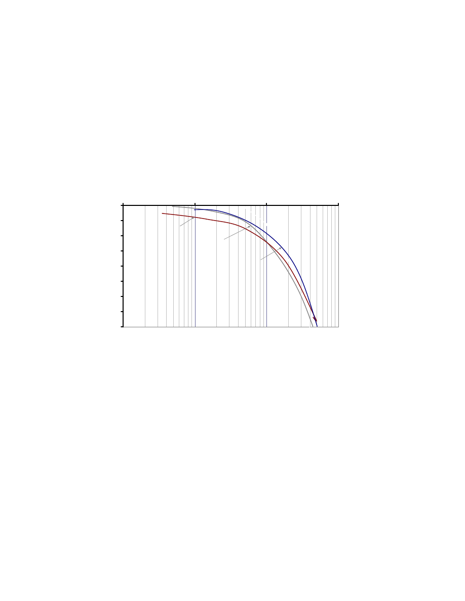
142
4.8.1. Strain rate effect on
ε- log σ’relationship
The CRS tests were performed at different strain rates (
ε) on three specimens
from the same Shelby tube sample recovered from the SH3 bridge at Clear Creek
Borehole B2 at a depth of 18 – 20 ft. The average strain rate was 0.16%/hr during the IL
test.
0
1
2
3
4
5
6
7
8
10
100
1000
10000
Vertical effective stress
σ
'
(psf)
A
xia
l stra
in
ε
(%
)
SR = 2 % / h
SR = 2 % / h
SR = 0.16 % / h
Fig. 4.26. Three
ε- log σ’ of CRS Tests Performed on Three Specimens from the
Same Shelby Tube Sample at Different Strain Rates.
The strain rate was increased from 0.16%/hr to 2%/hr (Fig. 4.26), a rate increase
of 12.5 time. The
ε- log σ’ relationships were very similar as shown in Fig. 4.26.
Consequently, the CRS test can be used for an accurate determination of the
preconsolidation pressure,
σ
p
- compression index, C
c
- recompression index, C
r
from the
obtained
ε –log σ’ or e –log σ’ curve (Fig. 4.27). At the strain rate of 0.025/ hr, the CRS
test was completed in less than 24 hrs, but the IL test was completed within 18 days.
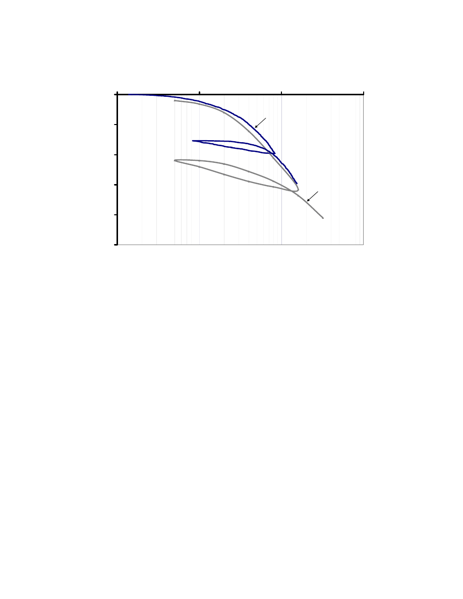
143
0
5
10
15
20
25
100
1000
10000
100000
Vertical effective stress
σ' (psf)
Axial strain
ε
(%)
IL
CRS
Fig. 4.27. Comparison of CRS Test (
ε= 0.025/hr) and IL Test ε – log σ’ Relationship
(Test Performed on Two Different Specimens from the Same Shelby Tube Sample
Recovered from SH3 at Clear Creek, Borehole B5 at 10 – 12 ft Depth).
4.8.2. Strain rate effect for C
v
The concern with the CRS consolidation test is the determination of a reliable
coefficient of consolidation C
v
since it depends on the strain rate of the test (Fig. 4.28).
The approach of Wissa et al. (1971) and of ASTM D 4186-86 is the specification of the
range of the pore water pressure ratio with the effective stress (
Δ
u/
σ
’) so that the
obtained values can comply with the ones obtained from the IL test. As was observed on
Fig. 4.29(a) even if the
ε – log σ’ curve from the CRS and IL test matched, their
respective C
v
–
σ
did not match, and the pressure ratio (Fig. 4.29(a)) did not comply with
the ASTM preferable values of 3% to 30%.
The coefficient of consolidation is defined as follows (Chapter 2)
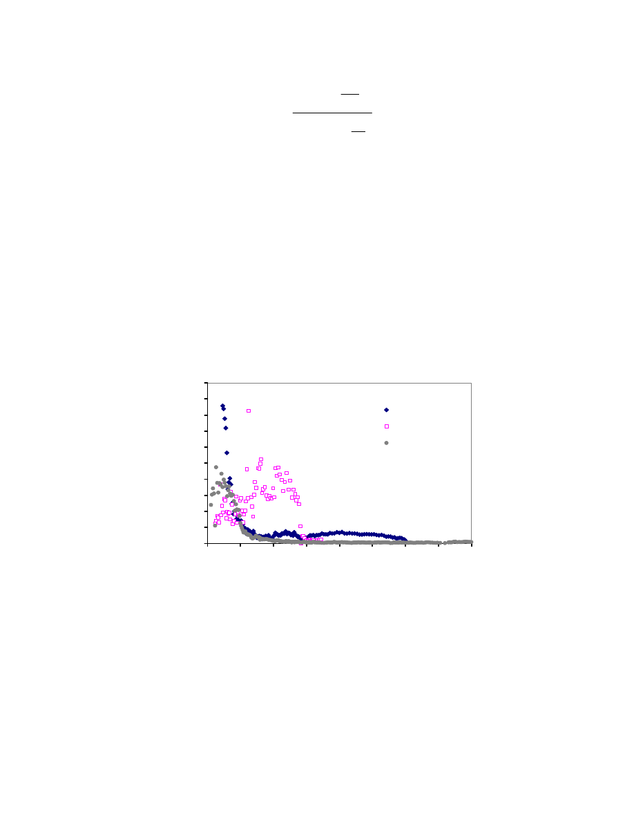
144
2
2
1
log
2 log 1
v
v
v
b
v
H
c
u
t
σ
σ
σ
⎡
⎤
⎢
⎥
⎣
⎦
= −
⎡
⎤
Δ
−
⎢
⎥
⎣
⎦
4-12
where:
σ
v1
= applied axial stress at time t
1
σ
v2
= applied axial stress at time t
2
H = average specimen height between t
1
and t
2
Δt = elapsed time between t
1
and t
2
u
b
= average excess pore pressure between t
2
and t
1
, and
σ
v
= average total applied axial stress between t
2
and t
1
.
0
200
400
600
800
1000
1200
1400
1600
1800
2000
0
2000
4000
6000
8000
10000
12000
14000
16000
Vertical effective stress
σ'
(psf)
C
v
(ft
2
/yr)
SR = 0.02/hr
SR = 0.0016/hr
SR = 0.02/hr
Fig. 4.28. Three C
v
-
σ’ of CRS Tests Performed on Three Specimens (CH Clay)
from the Same Shelby Tube Sample at Different Strain Rates.
Since the strain rate cannot be modified during the CRS consolidation test to fit
the required pressure ratio, a correlation needs to be developed for each type of soft clay
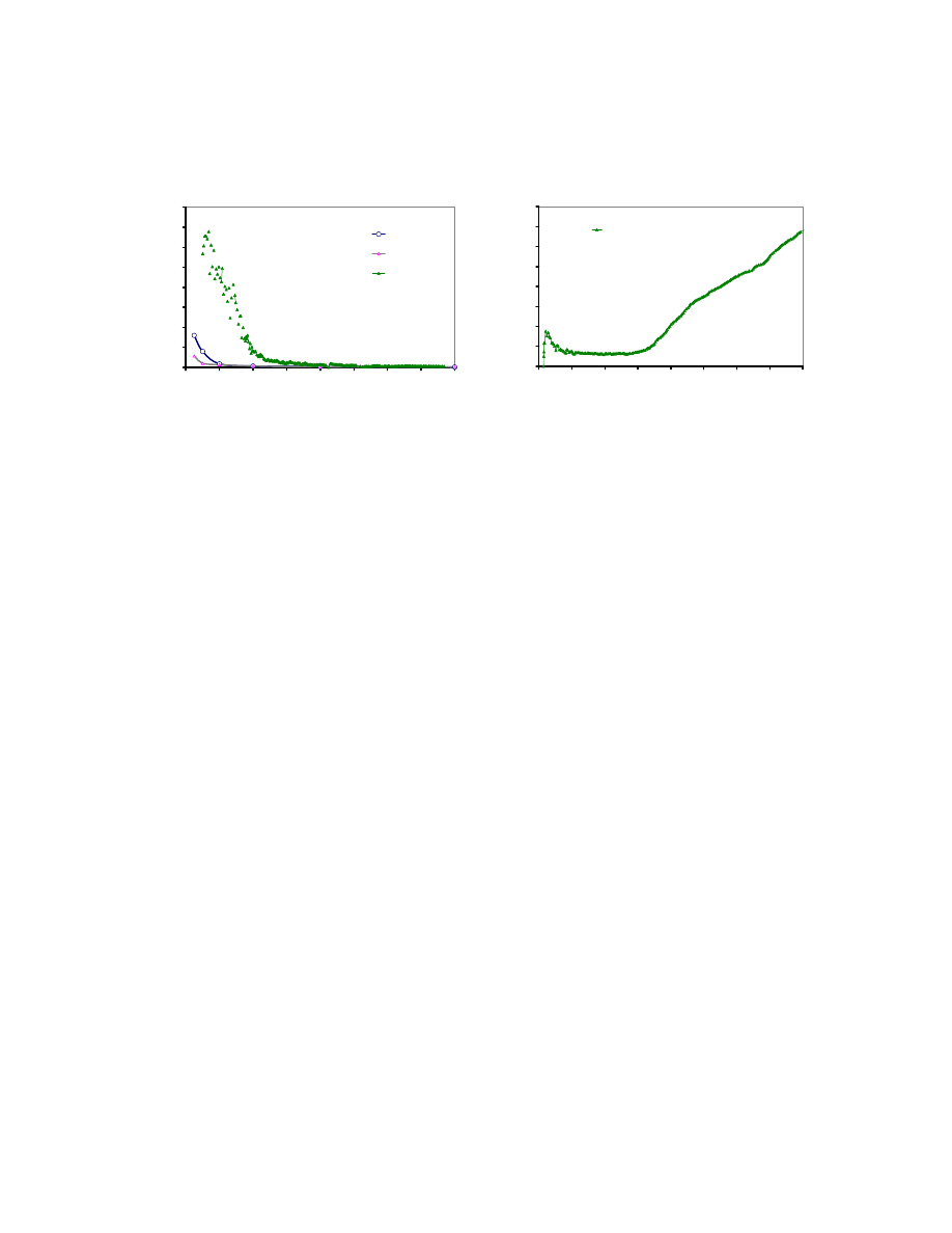
145
to define the convenient strain ε, as presented by Dobak (2003). This needs to be done for
the Houston clay.
0
200
400
600
800
1000
1200
1400
1600
0
2000
4000
6000
8000
10000
12000
14000
16000
Vertical effective stress
σ' (psf)
C
v
(ft
2
/y
r)
IL T90
IL T50
CRS (0.025/hr)
0.00
0.05
0.10
0.15
0.20
0.25
0.30
0.35
0.40
0
1000
2000
3000
4000
5000
6000
7000
8000
Vertical effective stress
σ' (psf)
P
ressu
re
ra
tio
CRS (0.025/hr)
a.)
b.)
Fig. 4.29. (a) Comparison of CRS Test (
ε= 0.025/hr) and IL Test C
v
–
σ
’ Curve (Test
Performed on Two Different Specimens from the Same Shelby Tube Sample
Recovered from SH3 at Clear Creek, Borehole 5 at 10 – 12 ft Depth); and (b)
Pressure Ratio vs. Vertical Effective Stress Corresponding to the CRS Test.
4.9. Summary
Over 40 consolidation tests and 50 unconfined compression tests were performed
to characterize the soils for SH3 and NASA Rd. 1 sites. The soil deposits are deltaic and
some properties had notable differences between the new (current study) and old data
(TxDOT reports).
Based on the laboratory study the following can be concluded:
(1) Since the increase in the in-situ stresses due to the embankment are relatively
small (generally less than the preconsolidation pressure), using the proper
recompression index is import. Since there is a large hysteresis loop during the
unloading-reloading of the soft CH clays, three recompression indices (C
r1
, C
r2
,
C
r3
) have been identified. Review of the TxDOT design indicates that there is no

146
standard procedure to select the recompression index. It is recommended to use
recompression index, C
r1
, to determine the settlement up to the preconsolidation
pressure.
(2) The consolidation parameters (C
c
, C
r
, C
v
) are all stress dependent. Hence, when
selecting representative parameters for determining the total and rate of
settlement, expected stress increases in the ground should be considered. In
estimating C
v
, the Casagrande’s T
50
gives a lower value than T
90
. C
v
is relatively
high before the preconsolidation pressure and notable reduction was observed
thereafter.
(3) The Constant Rate of Strain (CRS) test can be used to determine the consolidation
properties of clay soils. The rate used in the test influenced the coefficient of
consolidation.
(4) Linear and nonlinear relationships have been developed to represent the
compression index (C
c
) in terms of moisture content and unit weight.

147
5. FIELD STUDY
5.1. Introduction
In order to verify the applicability of the conventional 1-D consolidation theory to
predict the total and rate of settlement of embankments on soft clays, it was necessary to
monitor the settlement of embankments in the field. Based on the current condition and
accessibility, two embankments were selected. The selected locations are as follows:
(a) SH3 bridge embankment at Clear Creek (Project 3)
SH3 is a four-lane north-south highway (parallel to Interstate I45). The retaining
wall at Clear Creek on the east side showed tremendous distress with multiple cracked
panels and displaced joints. The embankment, about 14 years in service and sitting on
very soft clay, was bulging on the east side of SH3.
(b) NASA Rd. 1 at Taylor Lake (Project 4)
This is a six-lane east-west highway (perpendicular to Interstate I45) with the
three lanes supported on an embankment and the other three supported on piles across the
Taylor Lake. The pavement supported on the embankment has settled about 2.5 in. over
the years. This embankment has been in service for over seven years.
The field investigation for both sites included the following:
- site investigation
- field instrumentation and monitoring
- analyses of the data and comparing it to conventional consolidation theory.
It should be mentioned that in both locations there were no permanent reference
points to determine how much the embankments have settled over their service life.
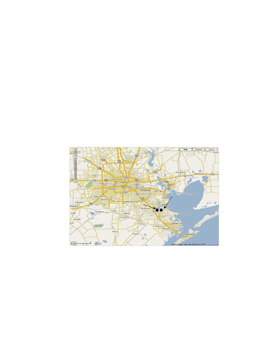
148
Hence, all the reported displacements (vertical and lateral displacements) are relative to
the new set references at the starting date of the monitoring.
As field monitoring devices, the following instruments were used:
- 30 to 40 ft long extensometers to measure vertical settlements
- inclinometer for lateral displacements
- piezometers for measuring the pore water pressure
- demec points for retaining wall movements
- retaining wall rotation monitoring marks
- tensiometer for measurement of suction pressure.
Fig. 5.1. Location of the Instrumented Embankment Sites.
5.2.
Site History and Previous Site Investigation
5.2.1. SH3 at Clear Creek Bridge and Clear Creek Relief Bridge (Project 3)
For widening the roadway and the bridges over Clear Creek and Clear Creek
Relief in 1971, seven soil borings were completed between September and October
SH3
NASA Rd. 1
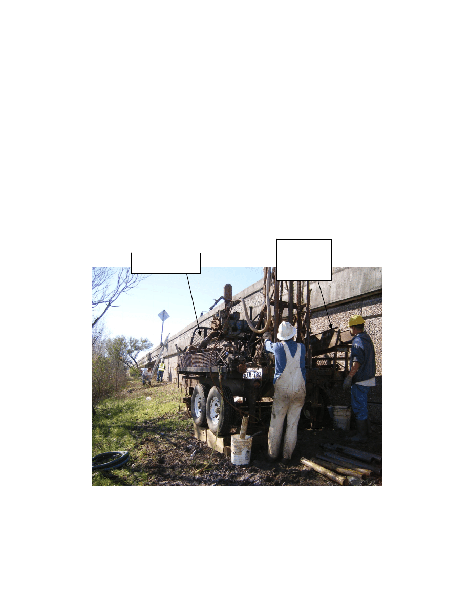
149
1965. In February, March, and September of 1984, seven new borings were
completed for the widening and elevating of the North Bridge (NB) roadway, for the
construction of retaining walls at the NB roadway and bridge approaches. Finally, one
boring was completed in November 1991 for the removal and replacement of the
South Bridge (SB) and for the construction of retaining walls at the SB Clear Creek
Relief bridge approaches in December 1993. A site visit in October 2006 showed that
the retaining wall panels have developed multiple cracks and the some of the panel
joints are misaligned indicating some form of ground movement.
Fig. 5.2. Sampling and Instrumenting at the SH3 Site (January 2007).
Retaining
Wall 2E of
Drilling machine
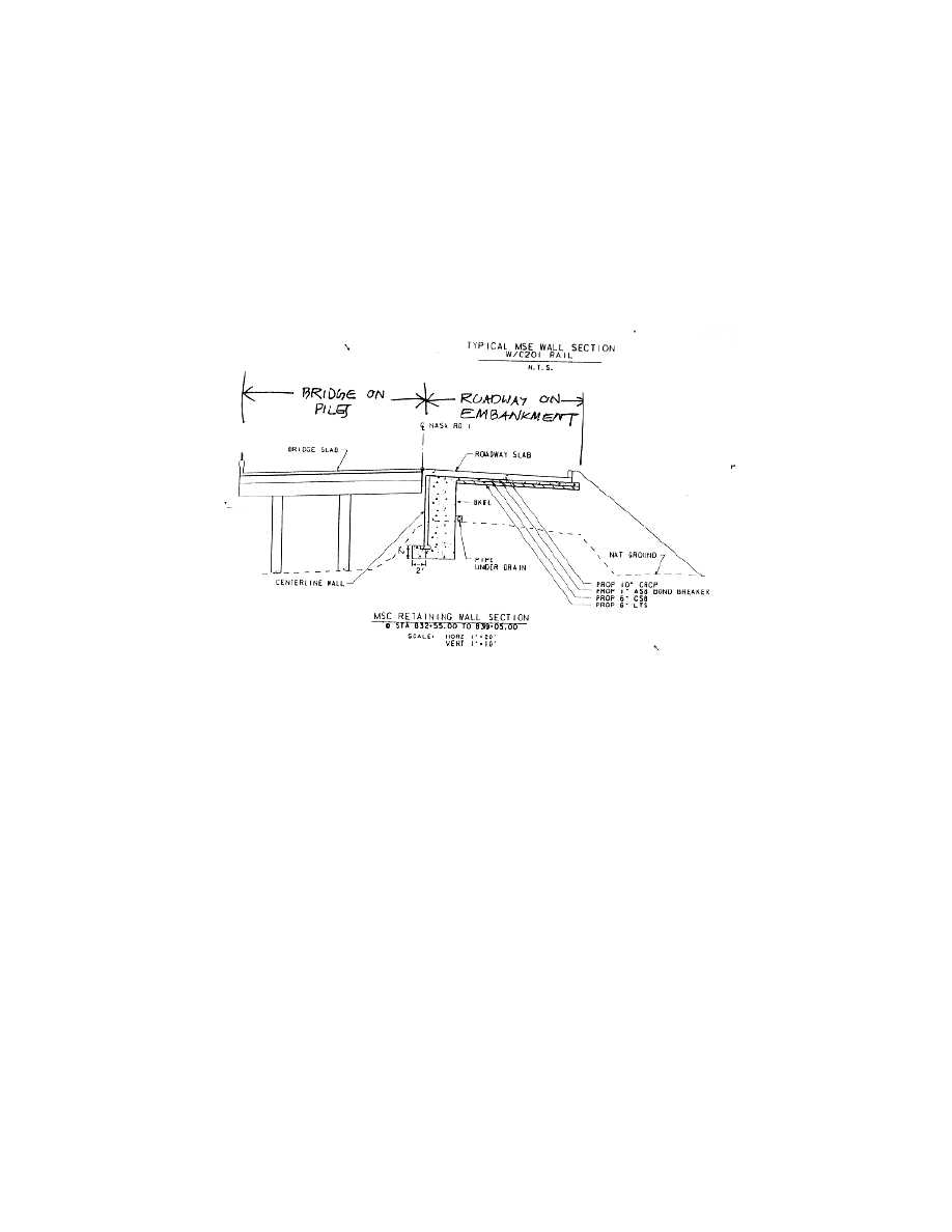
150
5.2.2. NASA Road 1 embankment at Taylor Lake
NASA Road 1 between Annapolis and Taylor Lake St. is a combination of a
bridge on piles and a roadway on an embankment (Fig. 5.3). Both the bridge and roadway
were built in 2000, and from the report of TxDOT, the roadway supported on
embankment has settled more than 2.5 in. since then.
Fig. 5.3. Cross Section of the NASA Road 1 Embankment (Project 4).
5.3. Instrumentation
5.3.1. Extensometer
The vertical settlement devices were developed and built at the University of
Houston. The devices measure the total settlement in the layer of height H (Fig.5.4).
When 0
1
1
<
−
=
Δ
initial
final
δ
δ
δ
(-) the soft soil layer is settling.
When
0
1
1
>
−
=
Δ
initial
final
δ
δ
δ
(+) the soft soil layer is expanding.
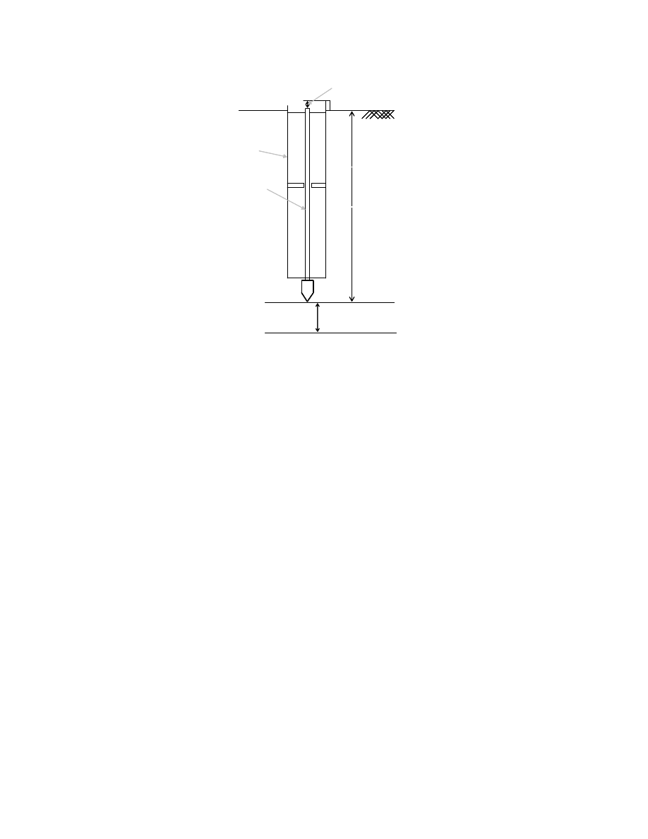
151
Fig. 5.4. Schematic of the Extensometer.
5.3.2. Operating
principles
of the inclinometer
Inclinometers are used to measure ground movement in unstable slopes and the
lateral movement of ground around ongoing excavations. Inclinometers also monitor the
stability of embankments, slurry walls, the disposition and deviation of driven piles or
drilled boreholes, and the settlement of ground in fills, embankments, and beneath
storage tanks. In this case, an inclinometer was used to monitor the lateral movement of
Boreholes B2 and B4. The movement is a reflection of the embankment stability.
An inclinometer casing was installed in the ground and grouted. The inclinometer
casing had four orthogonal grooves inside the casing (Fig 5.5(b)) designed to fit the
wheels of a portable inclinometer probe (Fig 5.5(a)). This probe, suspended on the end of
a cable connected to a readout device, was used to survey the inclination of the casing
with respect to vertical (or horizontal), and in this way to detect any changes in
inclination caused by ground movements.
Casing
Steel rod
δ
1
δ
2
Casing
Steel rod
δ
1
δ
2
Soft soil layer
of height H
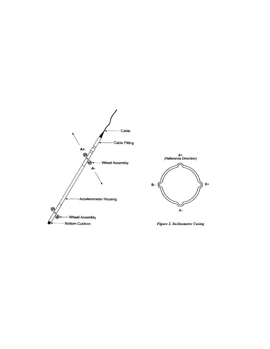
152
The inclinometer probe is composed of two accelerometers with their axes
oriented at 90°
to each other. The A axis is in line with the wheels with the B axis
orthogonal to it. Thus, during the survey, as the A+, A- readings were obtained; the
B+, B- readings were also recorded. The inclinometer probe used in this study was
manufactured by GEOKON Company. The readout box from the same company was
used to collect the data.
a)
b)
Fig. 5.5. (a) Inclinometer Probe (Geokon Inc 2007) and (b) Inclinometer Casing.
5.3.3. Principles of the demec points
Demec points are fixed metallic discs glued on any surface in different
configurations around a crack to monitor its movement (Fig. 5.6). In this study, demec
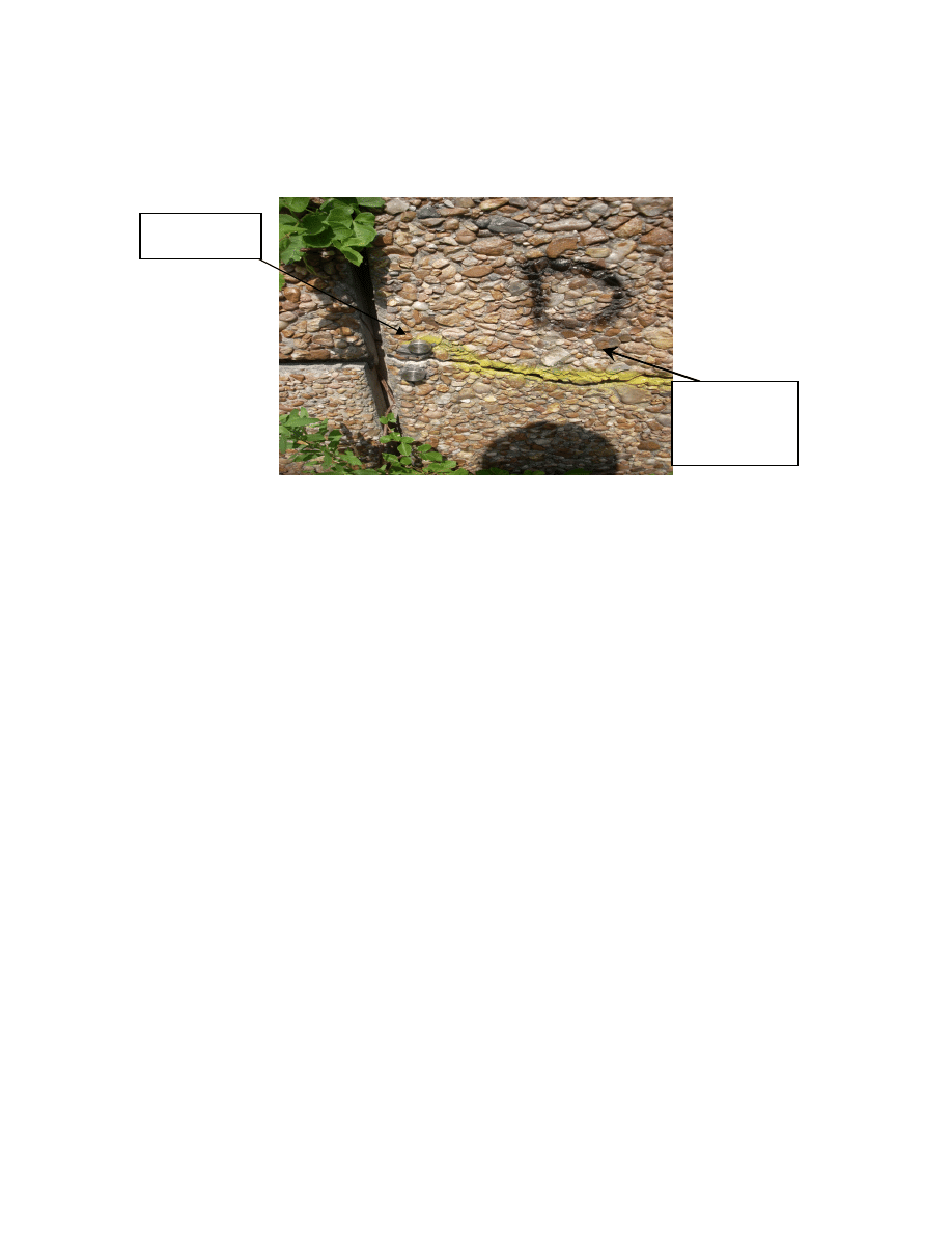
153
points were placed around the cracks on the retaining walls on SH3 to monitor their
movements.
Fig. 5.6. Demec on the Embankment Retaining Wall (Project 3).
5.3.4. Tensiometer
Direct measurement of matric suction in a borehole can be made by using a
tensiometer. A tensiometer consists of a tube with a porous ceramic tip on the bottom, a
vacuum gauge near the top and a sealing cap. When tensiometer is filled with water and
inserted into the soil, water can move into and out of the tensiometer through the
connecting pores in the tip. As the soil dries and water moves out of the tensiometer, it
creates a vacuum inside the tensiometer, which is indicated on the gauge. When the
vacuum created just equals the ‘Soil Suction,’ water stops flowing out of the tensiometer.
The dial gauge reading is then a direct measure of the force required for removing water
from the soil. If the soil dries further, additional water moves out until a higher vacuum
level is reached. Because water can move back and forth through the pores in the porous
ceramic tip, the gauge reading is always in balance with the soil suction.
Demec point
Crack on the
retaining
wall

154
5.4.
NASA Road 1 Embankment Instrumentation
The NASA Road 1 roadway between Annapolis and Taylor Lake St embankment
was instrumented in April 2007. A total of four borings were performed (UH1, UH2,
UH3, and UH4) and instrumented:
- Boreholes UH1 and UH3 were instrumented with sondex settlement devices.
- Boreholes UH2 and UH4 were each instrumented with a piezometer and an
extensometer.
5.5. SH3
Embankment
Instrumentation and Results
The SH3 embankment at Clear Creek was instrumented in January 2007 and was
been monitored for 18 months.
5.5.1. Site instrumentation
In January 2007, the field was (Fig. 5.7) instrumented as follows:
- Boreholes B2 and B4 were instrumented with inclinometer casings, up to 30 ft
deep, to monitor any lateral displacement of the embankment. Borings B2 and B4
were drilled, 5’4’’ and 5’6’’, respectively, from the embankment retaining wall.
- Boreholes B1, B3, and B5 were instrumented with extensometers made at the
University of Houston and piezometers, up to 30, 20, and 20 ft, respectively.
Boreholes B1, B3, and B5 were drilled at 5’1’’, 5’3’’, and 5’9’’, respectively,
from the retaining wall.
- Section 1 to 2 of 80 ft on the retaining wall (Fig. 5.7) had a number of cracks and
the main section was instrumented with demec points. Figure 5.8 shows the
schematic view of the instruments used.
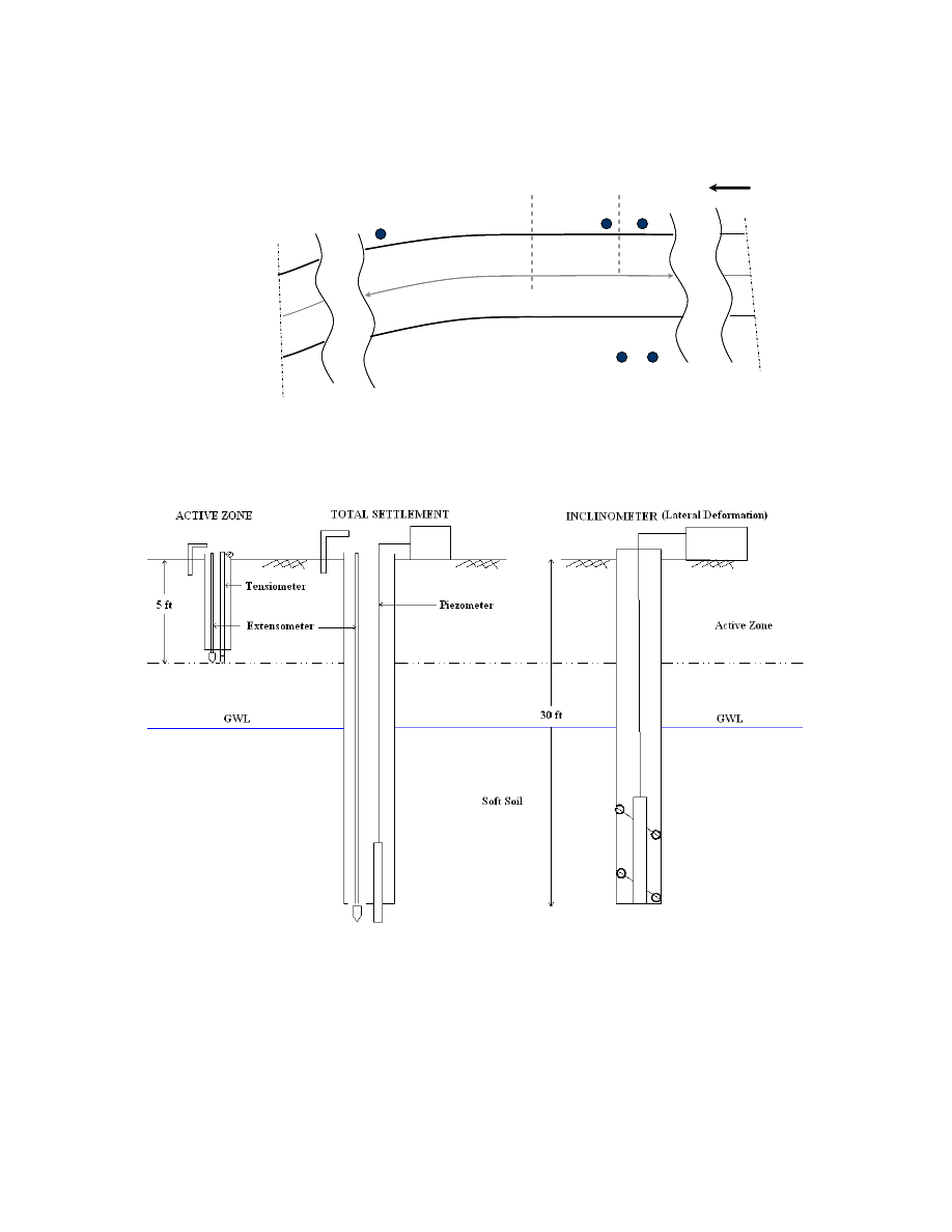
155
N
B1
B2
B4
B3
Clear
c
re
ek
Clear cre
ek reli
ef
840 ft
B5
N
B1
B2
B4
B3
Clear
c
re
ek
Clear cre
ek reli
ef
840 ft
B5
Fig. 5.7. Plan View of SH3 at Clear Creek with the New Boring Locations.
Fig. 5.8. Schematic View of Instruments Used in SH3.
80 ft
1
2
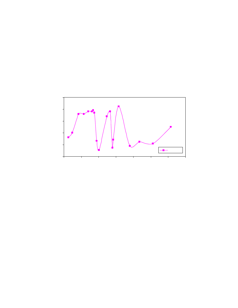
156
5.5.2. Monitoring results
East Side of SH3
• Groundwater Level
The groundwater level varied during the monitoring period as shown in Fig. 5.9. It
was influenced by the weather and the water level in Clear Creek. The ground water level
fluctuated by 20 in. (equivalent to 0.72 psi) over the monitoring period.
275
280
285
290
295
300
0
100
200
300
400
500
600
700
Days
W
at
er Head
(
in
.)
B1 GWL
Initial Day 1/26/2007
Fig. 5.9. Groundwater Table Variation with Time (Reference is the Bottom of the
Casing at 30 ft Deep as Reference at Boring B1).
• Inclinometer
In the presentation of the embankment lateral movement from the inclinometers
reading (Fig. 5.10), the Y-axis is the origin (Day 0 reading). The inclinometer reading
had accuracy of 6x10
-4
in.
From the Boring B2 reading, lateral displacement from Day 0 (installation day) to
Day 24 due to the installation and the cement grout setting time. (The cement grout
reached its optimum setting in 28 days). Inclinometer surveys were intermittently taken
for 490 days after setting of the grout. Figure 5.11 shows the lateral movement in the
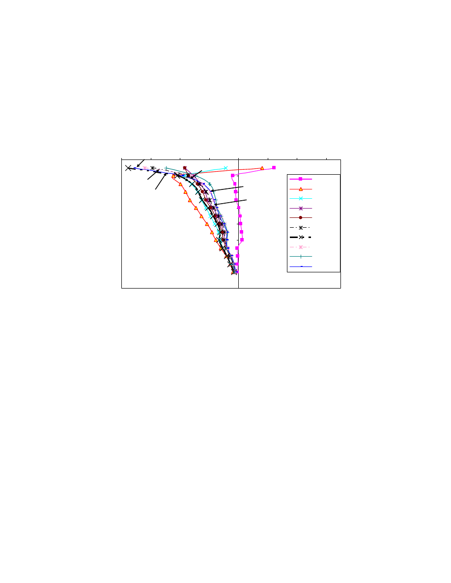
157
Borehole B2. From Fig. 5.10, it was determined that the soil moved laterally away from
the wall by about 0.4 in. in the top 5 ft and the lateral movement substantially diminished
below the 5 ft level to about 0.1 in. A displacement of 0.02 in. was recorded at a depth of
28 ft (Fig. 5.10).
6 Days
14 Days
24 Days
0
4
8
12
16
20
24
28
32
-0.4
-0.3
-0.2
-0.1
0
0.1
0.2
0.3
Change in Defelction (in)
D
ept
h (
ft
)
6 Days
14 Days
24 Days
47 Days
83 Days
161 Days
244 Days
265 Days
357 Days
490 Days
47
83
244
265
161
D
357
490
Initial Day 1/25/07
Fig. 5.10. Inclinometer Reading at Boring B2 (SH3).
• Extensometer Response
It must be noted that the extensometer will record the movement in the ground
(Active Zone and consolidation included) over a height of 30 ft. At Boring B1, the
ground initially expanded to 0.10 in. between the installation day and three months
thereafter. Then the ground settled to 1.0 in. (Fig. 5.11). After 300 days, the trend was
reversed. Over the period of measurement the extensometer readings were cyclic (heave
and settlement). A similar pattern of ground movement was measured in Borehole B3
(Fig. 5.12). The components of the settlements must be separated to better interpret the
results. The accuracy of the Vernier caliper used for the measurement was 0.004 in.
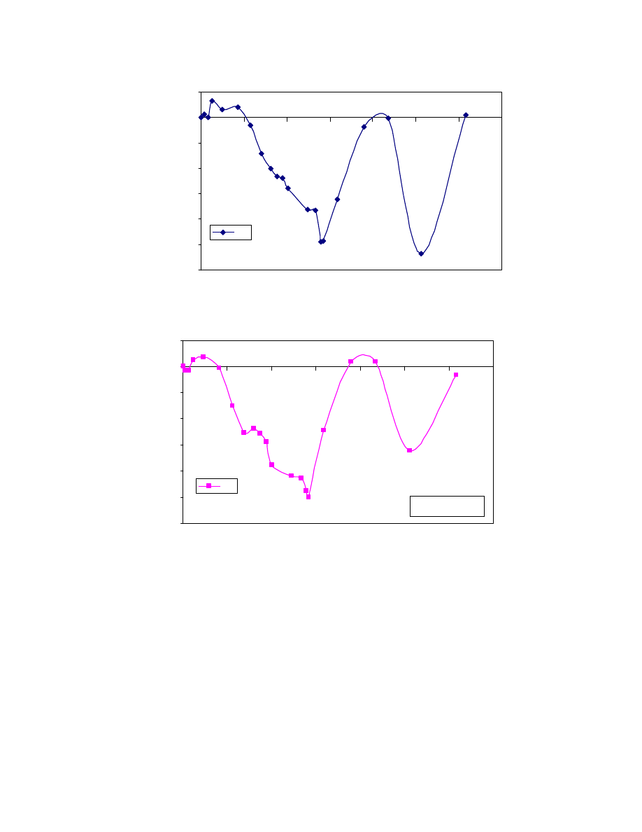
158
-1.20
-1.00
-0.80
-0.60
-0.40
-0.20
0.00
0.20
0
100
200
300
400
500
600
700
Days
Se
tt
le
m
ent
(
in)
B 1
-ve Settlement
+ve Heave
Fig. 5.11. Measured Relative Displacement with Time at Boring B1.
-1.20
-1.00
-0.80
-0.60
-0.40
-0.20
0.00
0.20
0
100
200
300
400
500
600
700
Days
Se
tt
le
m
ent
(
in
)
B 3
-ve Settlement
+ve Heave
Initial Day 1/26/07
Fig. 5.12. Measurement of Vertical Displacement with Time at Boring B3.
• Pore Water Pressure
The initial pore water pressure was 9.8 psi in Borehole B1, and it slightly
increased and decreased over 600 days of monitoring. The minimum and maximum pore
water pressures measured were 9.5 psi and 10.5 psi, respectively. It must be noted that
the hydrostatic pressure measured from the height of the water table was slightly higher
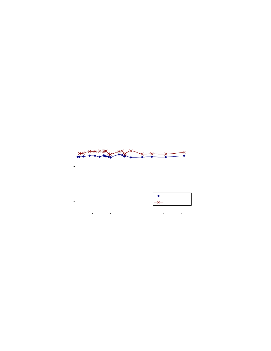
159
than the pore water pressure in the soil (Fig. 5.13). If the soil is consolidating the trend
should have been reversed.
Based on 1-D consolidation theory, the excess pore water pressure (u
i
) at a depth
of 30 ft is equal to 0.676
Δσ’ where Δσ’ is 475 psf (Table 3.16). Hence the excess pore
water pressure in the soil should be about 2.23 psi higher than the surrounding
hydrostatic pressure; but this was not the case and the pore water pressure measurement
did not indicate consolidation because the pore water pressure transducer was located in
the CL soil close to the bottom drainage. The accuracy of the piezometers was 0.002 psi.
0
2
4
6
8
10
12
0
100
200
300
400
500
600
700
Days
P
o
re
W
at
er
P
ress
u
re (
p
si)
B1
Hy. pressure B1
Initial Day 1/26/07
Fig. 5.13. Pore Water Pressure Variation with Time at Boring B1 (Project 3).
The initial pore water pressure was 6.15 psi in Borehole B3, and it slightly
increased and decreased over 600 days of monitoring. The minimum and maximum pore
water pressures measured were 5.8 psi and 6.5 psi, respectively. As measured in Borehole
B1, the hydrostatic pressure measured in Borehole B3 from the height of the water table
was slightly higher than the pore water pressure in the soil (Fig. 5.14). This may be due to
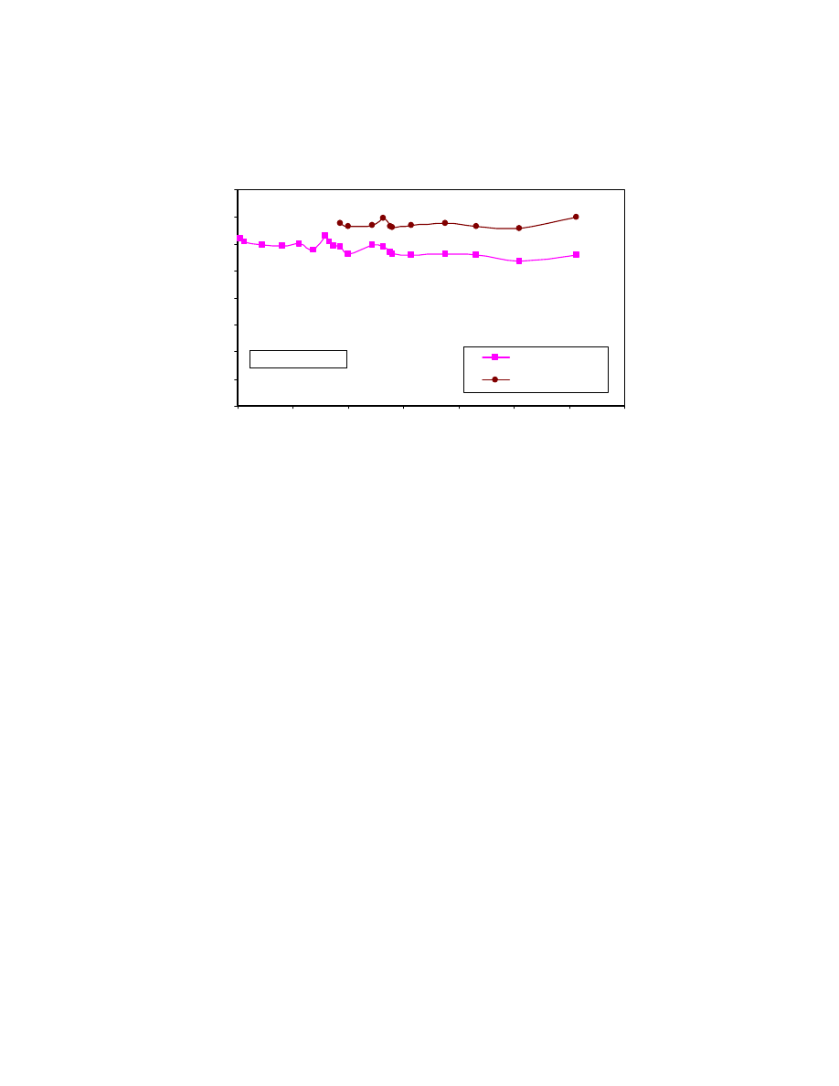
160
the fact that the pore water pressure transducer was located in the CL soil close to the
bottom drainage.
0
1
2
3
4
5
6
7
8
0
100
200
300
400
500
600
700
Days
Po
re
Wa
te
r Pre
ss
u
re
(
p
si
)
B3
Hy. Pressure B3
Initial Day 1/26/07
Fig. 5.14. Pore Water Pressure Variation with Time at Boring B3.
West Side of SH3
• Groundwater Level
The groundwater level varied during the monitoring period as shown in Fig. 5.15.
It was influenced by the weather and the water level in Clear Creek. The ground water
level fluctuated by 23 in. (equivalent to 0.83 psi) over the monitoring period.
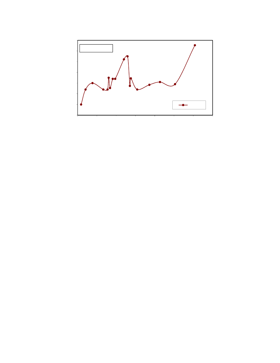
161
185
190
195
200
205
210
215
220
0
100
200
300
400
500
600
700
W
a
ter Head
(in
.)
Days
B5 GWL
Initial Day 1/31/07
Fig. 5.15. Water Table Variation with Time (Bottom of the Casing at 20 ft Deep as
Reference in Boring B5) (Project 3).
• Inclinometer
From the Boring B4 reading, the inclinometer casing had a lateral displacement
from Day 0 (installation day) to Day 23 due to the installation and the cement grout
setting time (the cement grout reaches its optimum setting in 28 days). A total lateral
displacement of 0.3 in. towards the embankment was recorded near the ground surface. A
relatively large lateral movement was observed in the top 5 ft as seen in Borehole B2.
The bottom of the casing, at 28 ft depth, can be considered static (Fig. 5.16). Very small
lateral movements in the soft soil region indicate no slope stability failure potential of the
embankment. This rules out the possibility of any failure that could also add to the
settlement of the embankment.
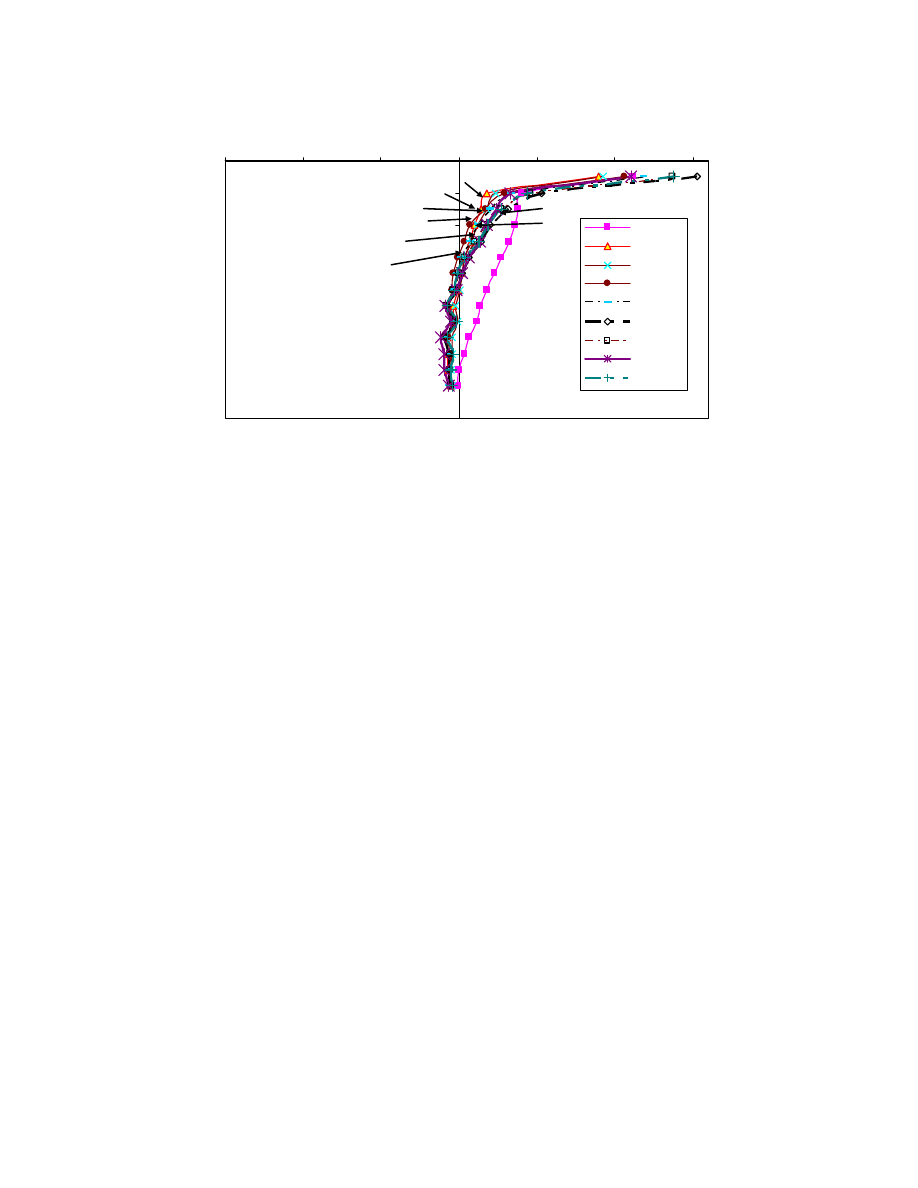
162
23 Days
89 Days
0
4
8
12
16
20
24
28
32
-0.3
-0.2
-0.1
0
0.1
0.2
0.3
Change in Deflection (in)
D
ep
th
(ft
)
23 Days
59 Days
89 Days
137 Days
177 Days
220 Days
241 Days
353 Days
486 Days
241
220
59
89
177
137
353
D
486
Fig. 5.16. Inclinometer Reading at Boring B4 (SH3).
• Extensometer Response
It must be noted that the extensometer will record the movement in the ground
(Active Zone and consolidation included) over a height of 20 ft. At Boring B5, the soil
settled 0.06 in. three months after installation (Fig. 5.17) and then expanded to less than
0.025 in. two months later. Over the period of measurement the extensometer readings
were cyclic (heave and settlement). A similar pattern of ground movement was measured
in Boreholes B1 and B3 (Fig. 5.11 and Fig. 5.12), but B5 had more fluctuation. The
components of the settlements must be separated to better interpret the results.
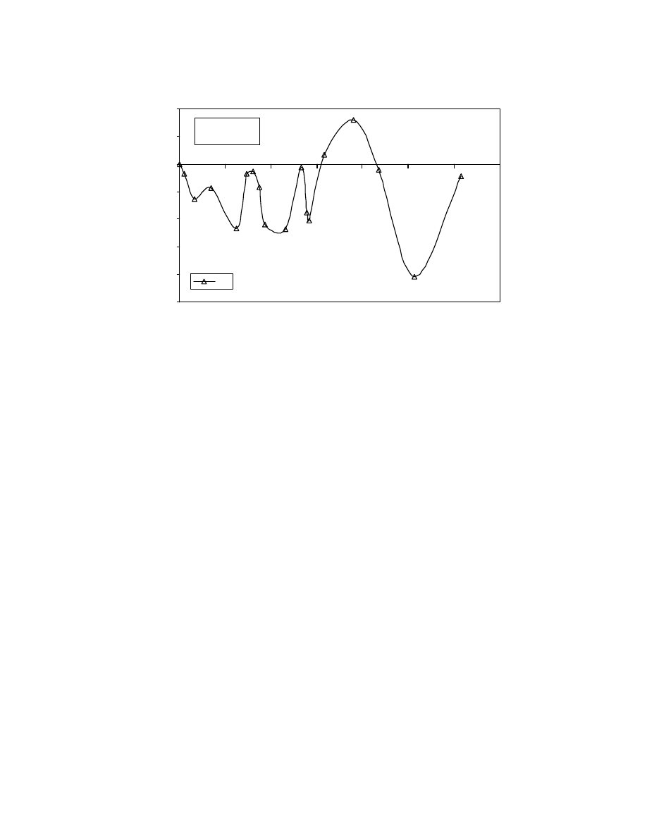
163
-0.25
-0.20
-0.15
-0.10
-0.05
0.00
0.05
0.10
0
100
200
300
400
500
600
700
Days
Se
tt
le
m
ent
(
in
)
B 5
Initial Day
2/8/2007
-ve Settlement
+ve heave
Fig. 5.17. Measured Relative Displacement with Time at Boring B5.
• Pore Water Pressure
The initial pore water pressure was 6.7 psi in Borehole B5, and it slightly
increased and decreased over 600 days of monitoring. The minimum and maximum pore
water pressures measured were 6.5 psi and 7.0 psi, respectively. It must be noted that the
hydrostatic pressure measured from the height of the water table was slightly higher than
the pore water pressure in the soil (Fig. 5.18). If the soil is consolidating, the trend should
have been reversed. This may be due to the fact that the pore water pressure transducer
would have been located close to the bottom drainage.
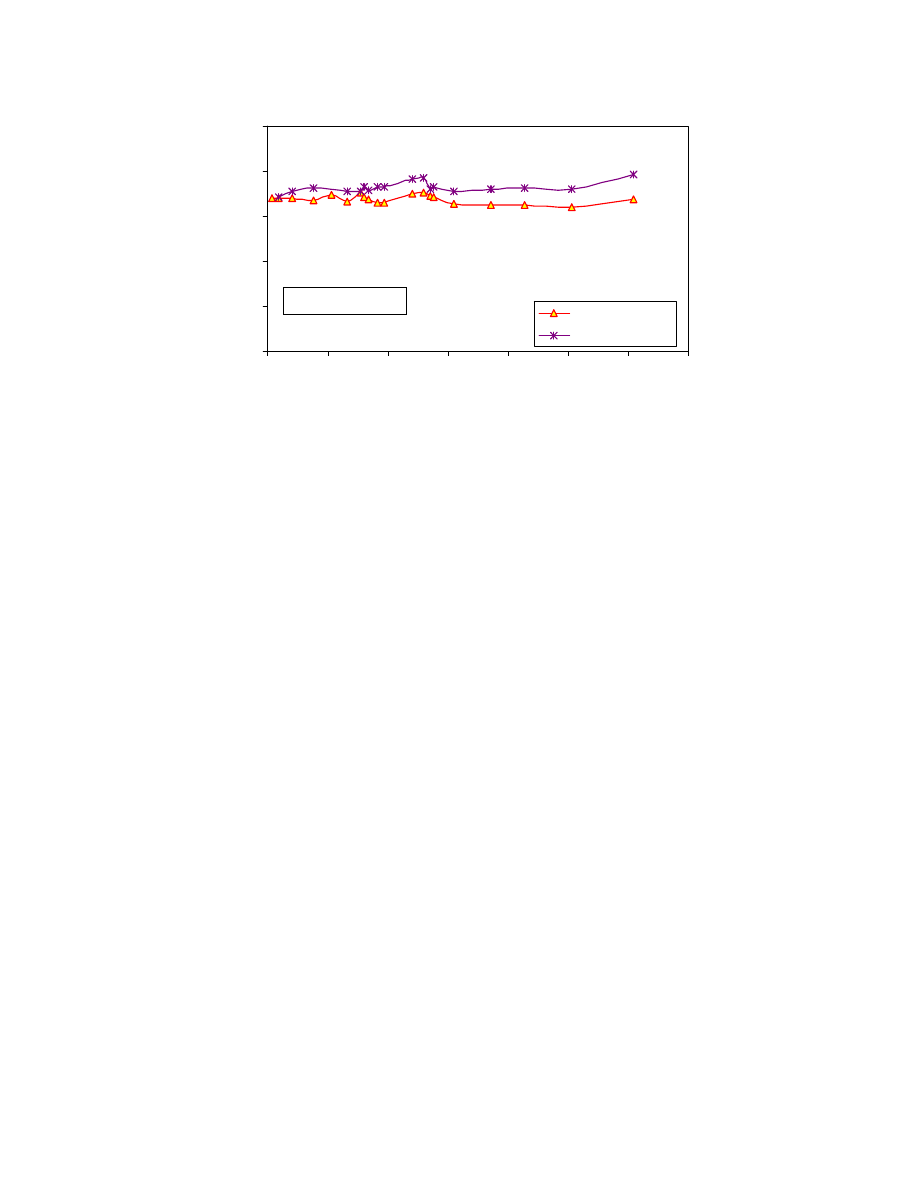
164
0
2
4
6
8
10
0
100
200
300
400
500
600
700
Days
P
o
re
W
at
er P
re
ss
u
re
(
p
si
)
B5
Hy. Pressure B5
Initial Day 1/31/07
Fig. 5.18. Pore Pressure Variation with Time at Boring B5.
• Tensiometer
Two tensiometers with extensometers were installed to a depth of 5 ft to measure
the matric suction and the settlement in the Active Zone near boreholes B2 and B3.
Fig. 5.19 shows the suction pressure measured. Fig. 5.20 shows the settlement measured
within the Active Zone.
During dry weather, the soil will shrink and the suction pressure will increase, the
ground will settle and the extensometer reading will be negative. During wet conditions,
suction pressure will decrease, the ground will swell and the extensometer reading will be
positive. The maximum suction measured during dry and wet weather conditions were
77 kPa and 10 kPa, respectively. The corresponding vertical settlement and swelling in
the soil measured by the extensometer were -0.2 in. (settlement) and 0.8 in. (ground
heave), respectively.
In order to understand the drying and wetting phenomena in the soil, the measured
data of rainfall and temperature are shown in the Fig. 5.21. The maximum average
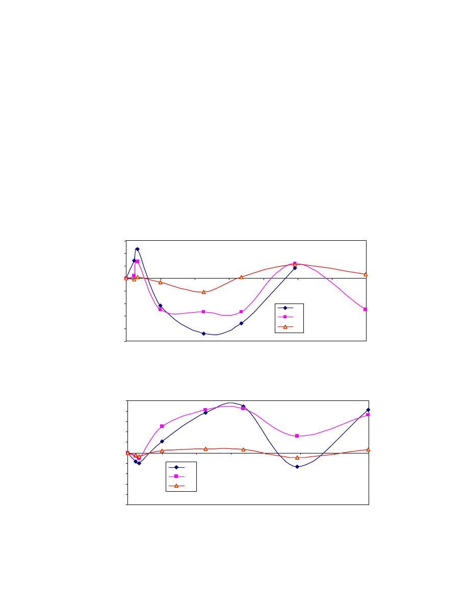
165
rainfall occurred during the months of January to March with average monthly
precipitation from 3 to 8 in. (75 mm to 200 mm). The 8-inch (200 mm) rainfall was
reported during Hurricane Ike. This was reflected in the reduced suction pressure and
swelling of the ground due to the increased moisture content. There was no extreme
effect on the suction pressure and swelling due to Hurricane Ike. The maximum
temperature was recorded during the months of May and June with temperatures of
84.7
o
F and 79.5
o
F, respectively. High temperature results in reduced ground moisture,
higher suction pressure, and settlement (Figs. 5.19 and 5.20).
-50
-40
-30
-20
-10
0
10
20
30
0
50
100
150
200
250
300
350
Days
Su
ct
io
n
Pr
es
su
re
(
kPa
)
B1
B3
B5
OCT NOV DEC FEB APR JUN SEP
Fig. 5.19. Change in Suction Pressure.
-1
-0.8
-0.6
-0.4
-0.2
0
0.2
0.4
0.6
0.8
1
0
50
100
150
200
250
300
350
Days
S
ettl
em
en
t (i
n
.)
B1
B3
B5
Fig. 5.20. Variation in Settlement in Active Zone.
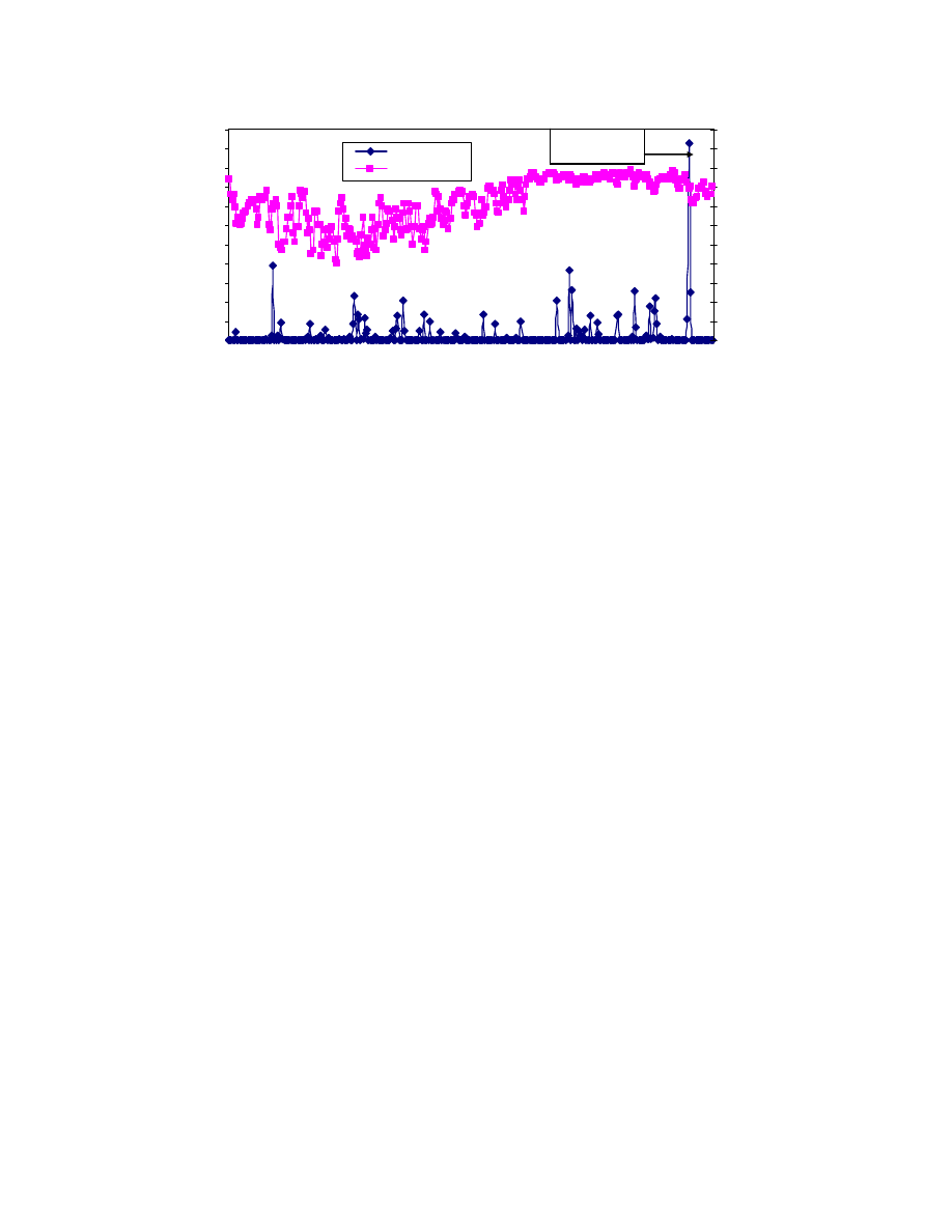
166
0
20
40
60
80
100
120
140
160
180
200
220
0
50
100
150
200
250
300
350
Days
P
re
cipit
at
ion
(
m
m
)
0
10
20
30
40
50
60
70
80
90
100
110
T
em
p
er
at
u
re (
F
)
Rainfall
Temperature
Hurricane Ike
10/132008
Fig. 5.21. Measured Rainfall and Temperature for the Houston (www.weather.gov).
• Consolidation Settlement
As mentioned before total settlements were measured using the long
extensometers in Boreholes B1, B3 and B5. The consolidation settlement was determined
by subtracting the Active Zone movement from the total settlement. Figure 5.22 shows
the measured consolidation settlement over a period of a year and the consolidation
settlement varied from 0.06 to 0.10 in.
Conventional
consolidation
theory predicted continuous consolidation settlement
at this site. This was observed at the SH3 at Clear Creek embankment. Consolidation
settlement measured over a period of 12 months at the edge of the embankment at the
Clear Creek Bridge at SH3 varied from 0.08 to 0.10 inches after making the correction
for the Active Zone. Based on the conventional consolidation theory, the settlement
between 14 and 15 years will be in the range of 0.02 in. to 0.03 in. (Chapter 3), which
was close to what was measured in the field. The difference between the measured and
predicted consolidation settlement could be partly due to the Active Zone correction.
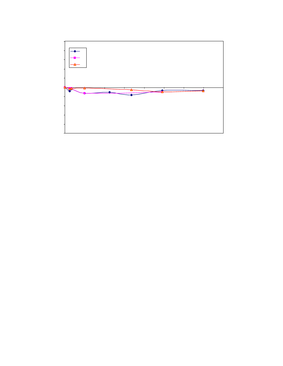
167
Fig. 5.22. Variation of Consolidation Settlement (Project 3).
• Demec points
Four of the configurations in Fig. 5.23(a) and 11 configurations 5.23(b) were
installed. Eighteen months after the installation of the demec points on the retaining wall,
particularly in Section 1-2 (Fig. 5.7), the measured changes in distance between the
cracks and the retaining wall panels were between -0.08 in. and 0.12 in. (Fig. 5.24 and
Fig. 5.25). The changes in the crack opening and closing over time can be related to the
movement in the Active Zone. Compared to the Active Zone movement, the
consolidation settlement is small and will have minimal effect on the panel cracking. The
accuracy of the Vernier caliper used for measurement was 0.001 in.
-1
-0.8
-0.6
-0.4
-0.2
0
0.2
0.4
0.6
0.8
1
0
50
100
150
200
250
300
350
400
Days
S
ett
le
m
ent (i
n.
)
B1
B3
B5
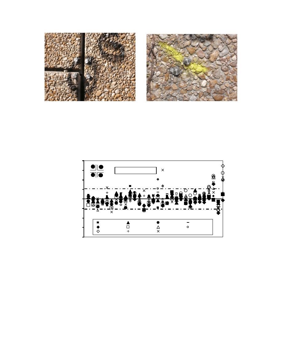
168
a)
b)
Fig. 5.23. Picture View of Demec Points on the Wall: a) for Wall Panel Displacement
Monitoring and b) Crack Opening Monitoring (Project 3).
-0.16
-0.12
-0.08
-0.04
0.00
0.04
0.08
0.12
0.16
Di
sp
la
ce
m
en
t (i
n)
3/13/2007
4/18/2007
5/18/07
6/13/07
7/5/2007
7/18/2007
8/1/2007
8/14/2007
9/26/2007
2/7/2008
6/19/2008
POINT C
POINT Q
POINT N2
POINT L
POINT G
1-2
1-3
4-1
3-4
2-3
2-
4
1-2
1-
3
4-1
3-4
2-
3
2-4 1-2
1-3
4-1
3-
4
2-
3
2-4 1-
2
1-
3
4-1
3-4
2-3
2-4
1-2
1-3
4-
1
3-4
2-3
2-4
1
4
3
2
Initial Reading: 12/10/06
Fig. 5.24. Relative Displacements of the Wall Panels along the Embankment.
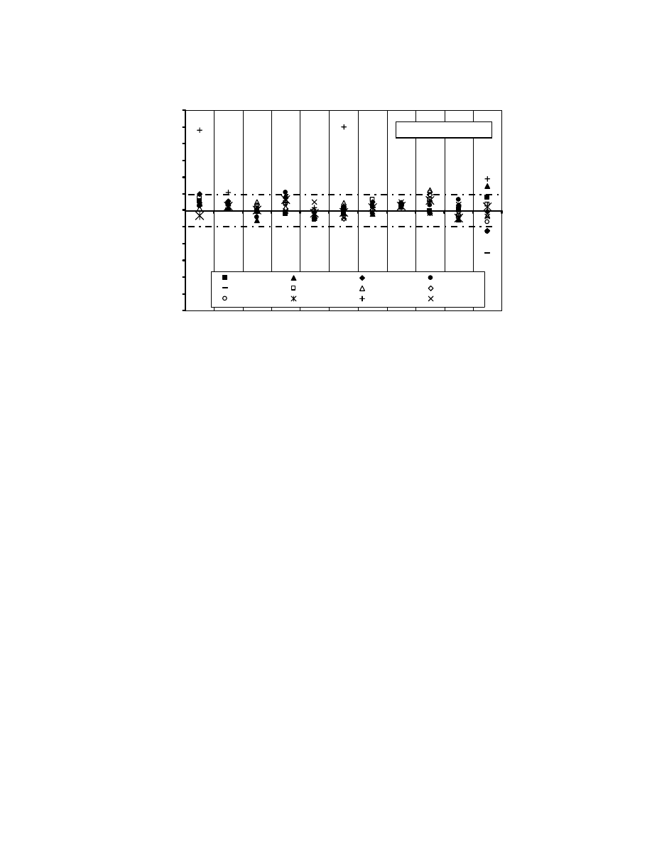
169
-0.24
-0.20
-0.16
-0.12
-0.08
-0.04
0.00
0.04
0.08
0.12
0.16
0.20
0.24
D
is
pl
ac
em
ent (
in)
1/25/2007
3/13/2007
4/18/2007
5/18/2007
6/13/2007
7/5/2007
7/18/2007
8/1/2007
8/14/2007
9/26/2007
2/7/2008
6/19/2008
POINT
A
POINT
B
POINT
A2
POINT
D
POINT
E
POINT
H
POINT
I
POINT
K
POINT
O
POINT
R
POINT
T
Initial Reading: 12/10/06
Fig. 5.25. Change in the Crack Opening along the Wall.
• Wall rotation
The wall was bulging at a few locations on the east side of SH3. The changes in
the vertical alignment (rotation angle) of the panels were measured using a digital level.
Eleven of the wall rotation monitoring marks were placed along the retaining wall
(Figs. 5.26 and 5.27). The wall rotation at all 11 marks, within 550 days of monitoring
varied between -1.0° and 1.0°, and the accuracy of the leveler was 0.1°. The wall panel
rotations could be better related to the movements in the Active Zone.
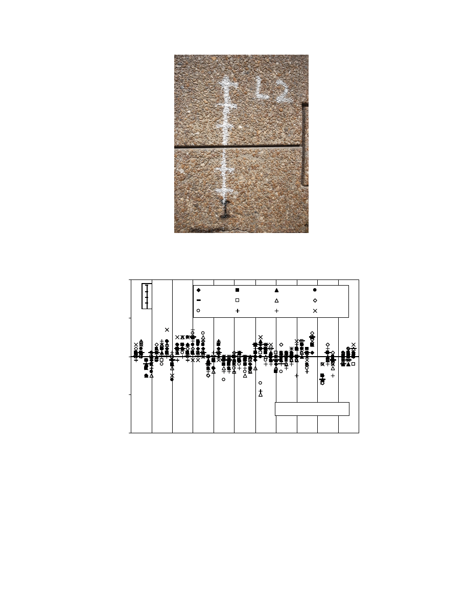
170
Fig. 5.26. View of L2 Rotation Monitoring Mark Line on the Retaining Wall.
-2
-1
0
1
2
Intervals
A
n
g
u
la
r D
isp
lacem
en
t (
°)
1/25/2007
3/13/2007
4/18/2007
5/18/2007
6/13/2007
7/5/2007
7/18/2007
8/1/2007
8/14/2007
9/26/2007
2/7/2008
6/19/2008
L1
L2
L3
L4
L5
L6
L7
L8
L9
L10
L11
Initial Reading: 12/10/06
Fig. 5.27. Change in Wall Rotation Monitoring Mark Readings along the Retaining
Wall.

171
5.6.
NASA Road 1 (Project 4)
Piezometer and Ground Water Table Level Readings
Two piezometers were installed in Boreholes UH-2 and UH-4. The depth of UH-2
was 30 ft and Borehole UH-4 was 40 ft. At these boreholes, ground water levels were
also monitored.
At Borehole UH-2, the initial pore pressure was 9.3 psi and it tended to fluctuate
slightly over the monitoring period (Fig 5.28(a)). The minimum and maximum pore
pressures measured were 8.5 and 9.5 psi, respectively. As observed before, the
hydrostatic pressure was higher than the pore water pressure in the soil. The pore water
pressure and hydrostatic trends were reversed at Borehole UH-4 (Fig 5.28(b)) and the
difference was over 1.5 psi, representing the consolidation theory prediction.
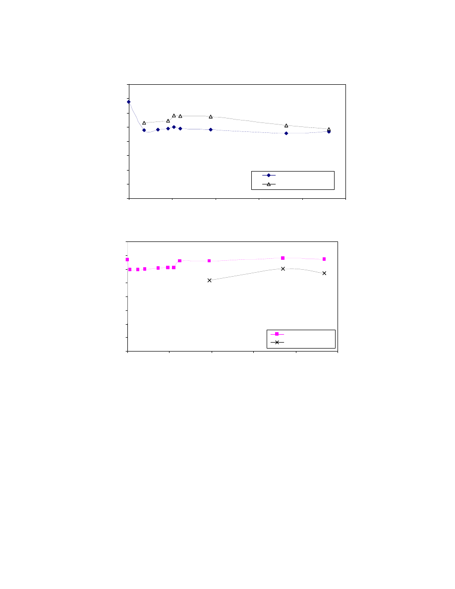
172
0
2
4
6
8
10
12
14
16
0
100
200
300
400
500
Days
P
res
su
re
(
p
si
)
UH-2
Hy. Pressure UH 2
(a)
0
2
4
6
8
10
12
14
16
0
100
200
300
400
500
Days
P
res
su
re
(
p
si
)
UH-4
Hy. Pressure UH 4
(b)
Fig. 5.28. Piezometer Readings at (a) Borehole UH-2 and (b) Borehole UH-4.
Extensometer Results
Extensometers were placed with the piezometers, at Boreholes UH-2 (20 ft
embankment + 10 ft into the ground) and Borehole UH-4 (20 ft embankment + 20 ft into
the ground). The Active Zone was not an issue as in the case of SH3 (Fig. 5.29).
According to the final readings, 0.21-in. and 0.18-in. settlements were observed at
Borehole UH-2 and Borehole UH-4, respectively.
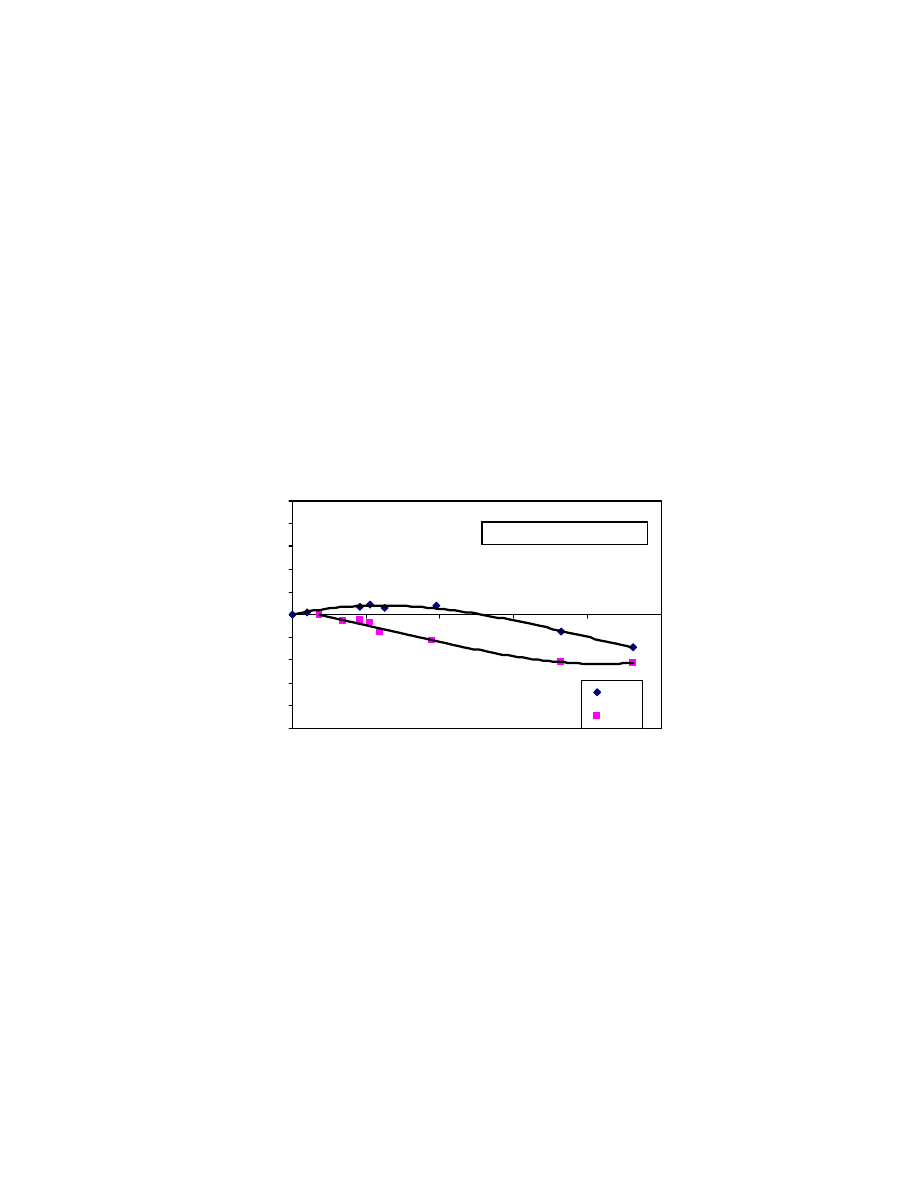
173
Conventional consolidation theory predicted continuous consolidation settlement
at this site. This was observed at this location. The consolidation settlement measured
over a period of 12 months below the embankment at the Taylor Bridge at NASA Rd. 1
for a thickness of 20 ft (Borehole UH 4) was 0.18 in., and the predicted settlement using
the 1-D consolidation theory was 0.21 in. (Chapter 3). For a thickness of 10 ft at
Borehole UH 2, the consolidation settlement was 0.21 in., while the predicted settlement
based on the consolidation theory (between 7 and 8 years) was 0.12 in. (Chapter 3). The
agreement between measured and predicted consolidation settlements was good.
Fig. 5.29. University of Houston’s Settlement Measurement Set-Up Readings.
5.7.
Summary and Discussion
Two highway embankments that are in service were instrumented and monitored
to determine the settlement due to consolidation of the soft clays supporting the
embankments. The field instrumentation included extensometers, piezometers,
inclinometers, demec points, and tensiometers. The embankments were monitored over
period of 500 days. Since both of the embankments were next to a large body of water
-0.50
-0.40
-0.30
-0.20
-0.10
0.00
0.10
0.20
0.30
0.40
0.50
0
100
200
300
400
500
Days
Se
ttl
em
en
t (i
n)
UH 4
UH 2
Initial Reading 5/17/2007
-ve Settlement
+ve Heave

174
(creek and lake), the changes in weather affected the ground water table height. During
the study period, the water table fluctuated by as much as 35 in. At SH3 at Clear Creek,
the embankment settlement was measured at the edges, and at NASA Road 1, it was
measured under the embankment. Based on the field monitoring and analyses following
conclusions are advanced:
(1) The maximum lateral movement recorded by the inclinometers was 0.4 in. near the
ground surface. The lateral movement was less than 0.1 in. below a depth of 5 ft. Lateral
measurements in the soft soils showed no sign of embankment stability failure.
(2) The largest vertical movements over time were measured in the top 5 ft of the Active
Zone at SH3 at Clear creek. Changes in the Active Zone were monitored using a
tensiometer (suction pressure) and an extensometer (vertical movements). During the
period of monitoring, a maximum swelling of 0.8 in. and settlement of 0.2 in. were
measured.
(3) Conventional consolidation theory predicted continuous consolidation settlement at
these two sites. This was observed at both of the test locations. The consolidation
settlement measured over a period of 12 months at the edge of the embankment at the
Clear Creek Bridge at SH3 was between 0.08 and 0.10 in. after making the correction for
the Active Zone. Based on the conventional consolidation theory, the settlement between
14 and 15 years will calculate to be 0.02 to 0.03 in., which was close to what was
measured in the field. The consolidation settlement measured at the NASA Rd.1 bridge

175
site for the 20 ft thickness was 0.18 in. during the 12 month period. The magnitude of the
consolidation settlement predicted for this site by the conventional theory, between 7 and
8 years, was about 0.21 in. The consolidation settlement measured at the NASA Rd.1
bridge site for the 10 ft thickness was 0.21 in. during the 12 month period. The magnitude
of consolidation settlement predicted for this site by the conventional theory, between 7
and 8 years, was about 0.12 in. The 1-D consolidation theory predicted the settlement
well.
(4) The piezometer readings, in three of the four cases, were below the surrounding
hydrostatic pressure determined from the groundwater table height. During consolidation,
piezometer readings should be higher than the surrounding hydrostatic pressure. This
could be partly due to the fluctuation in the ground watertable.


177
6. CONCLUSIONS
AND
RECOMMENDATIONS
The prediction of consolidation settlement magnitudes and settlement rates is a
challenging task, and it has been attracting the attention of numerous researchers since
the inception of consolidation theory by Terzaghi in early 1920s. The challenges mainly
come from the uncertainties about the subsurface conditions, soil disturbances during
sampling and preparations of samples for laboratory testing, interpretations of laboratory
test data, and assumptions made in the development of the 1-D consolidation theory
(Duncan 1993; Olson 1997; Holtz and Kovacs 1981). Since the soft soil shear strength is
low, the structures on the soft soils are generally designed so that the increase in the
stress is relatively small and the total stress in the ground will be close to the
preconsolidation pressure. Hence there was a need to investigate methods to better
predict the settlement of embankments on soft soils.
There are several field and laboratory test parameters that are used in the
settlement analysis and are very important in the prediction of consolidation settlement
magnitudes and settlement rates. Determining the thickness of the in-situ soil that will be
influenced by the new construction and estimating the increases in stresses are important.
The laboratory test parameters such as compression index, C
c
, recompression index
(or swell index), C
r
(or C
s
), coefficient of consolidation, C
v
, and preconsolidation
pressure and their variability within the in-situ soils are important. In addition to
engineering judgment used in determining some of these parameters, the geological
nature of the soil deposits must be considered. Since the soils in the Texas Gulf Coast
region are deltaic deposits, large variations in properties can be expected.

178
In this study, the procedure used by TxDOT to estimate the total and rate of
settlement were reviewed. In order to verify the prediction methods, two highway
embankments on soft clay with settlement problems were selected for detailed field
investigation. Soil samples were collected from 9 boreholes for laboratory testing and
over 40 consolidation tests and 50 unconfined compression tests were performed on the
clay samples. The embankments were instrumented and monitored for 20 months to
measure the vertical settlement, lateral movement, and changes in the pore water
pressure. Based on this study the following can be concluded:
(1) The method currently used by TxDOT to determine the increase in in-situ stress is
comparable to the Osterberg method and is acceptable. The approach used by the
TxDOT to determine the preconsolidation pressure is acceptable (Casagrande
Method).
(2) Total settlement has been estimated by TxDOT based on very limited
consolidation tests. Since the increase in in-situ stresses due to the embankment is
relatively small (generally less than the preconsolidation pressure), using the
proper recompression index is import. Since there is a hysteresis loop during the
unloading-reloading of the soft CH clays, three recompression indices (C
r1
, C
r2
,
and C
r3
) have been identified. Review of the TxDOT design indicates that there is
no standard procedure to select the recompression index. It is being recommended
to use recompression index C
r1
to determine the settlement up to the
preconsolidation pressure.
(3) The procedure used by TxDOT to determine the rate of settlement is not
acceptable. In determining the rate of settlement, the thickness of the entire soil

179
mass must be used with the average soil properties and not the layering method.
The layered approach will not satisfy the drainage conditions needed to use in the
time factor formula and determine the appropriate coefficient of consolidation.
(4) The consolidation parameters (C
c
, C
r
, C
v
) are all stress dependent. Hence, when
selecting representative parameters for determining the total and rate of
settlement, expected stress increases in the ground should be considered.
(5) The 1-D consolidation theory predicted continuous consolidation settlement in
both the embankments investigated. The predicted consolidation settlements were
comparable to the consolidation settlement measured in the field. The pore water
pressure measurements in some cases did not indicate consolidation because they
may have been located close to the bottom drainage. In one case, it indicated
excess pore water pressure and hence consolidation was in progress.
(6) The Active Zone influenced the movements in the edge of the embankments.
Movements in the Active Zone influenced the crack movements in the retaining
wall panels.
(7) Constant Rate of Strain (CRS) test can be used to determine the consolidation
properties of clay soils. The rate used in the test influenced the coefficient of
consolidation.
Based on this study, the following recommendations are advanced:
(1) The thickness of the soil mass that is influenced by the embankment construction
must be determined based on in-situ stress increase and the consistency of the soil
below the embankment. The TCP and undrained shear strength should be used to
determine the consistency of the soil.

180
(2) Since relatively large variations in the properties can be expected in the deltaic
deposits, soil samples must be obtained for an adequate and representative
number of boreholes to determine the consolidation properties.
(3) Determining the rate of settlement approach must be corrected.
(4) Based on only two already existing embankment settlements monitoring in the
field, 1-D consolidation theory can be used to determine the total and rate of
consolidation.
(5) Active Zone effects must be considered in designing the edge of the embankment
including retaining walls.
(6) CRS must be considered as an alternative method to determine the consolidation
properties.
(7) The number of consolidation tests used to determine the consolidation properties
of the soils in each project must be increased. Due to the variability in the
properties of deltaic deposited clay soils, it is recommended to use one
consolidation test for each 5 ft within the soft soil layers for settlement analyses.

181
7. REFERENCES
ASTM International. (2002). “Annual Book of ASTM Standards,” Edition 4, 2002,
Vol. 04.08, Soil and Rock (I).
Azzouz, A.S., Krizek, R.J., and Corotis, R.B. (1976). “Regression analysis of soil
compressibility.” Soil and Foundation, JSSMFE, Vol. 16, No. 2, pp. 19-29.
Bjerrum, L. (1974). “Problems on Soil Mechanics and Construction on Soft Clays.”
Norwegian Geotechnical Institute, Publication No. 110. Oslo.
Boussinesq, J. (1883). “Application des Potentials à L’Etude de L’Equilibre e du
Mouvement des Solides Elastiques”, Gauthier-Villars, Paris.
Casagrande, A. and Fadum, R. E. (1940). “Notes on Soil Testing for Engineering
Purposes,” Harvard University Graduate School of Engineering Publication No. 8
Chung, S.G., Giao, P.H, Nagaraj, T.S. and Kwag, J.M. (2002). “Characterization of
Estuarine Marine Clays for Coastal Reclamation in Pusan, Korea.” Marine
Georesources and Geotechnology, 2000, Vol. 20, pp. 237-254.
Cudny, M. (2003). “Simple multi-laminate model for soft soils incorporating structural
anisotropy and destructuration,” In P.A. Vermeer, H.F. Schweiger, M. Karstunen
& M. Cudny (ed.), Proc. Int. Workshop on Geotechnics of Soft Soils : Theory and
Practice, Noordwijkerhout. VGE.
Das, B.M. (2006). “Principles of Geotechnical Engineering,” Brooks/Cole Pub Co. 589 p.
Dobak, P. (2003) “Loading Velocity in Consolidation Analysis.” Geotechnical Quarterly,
2003, Vol. 47, No. 1, pp. 13-20.
Duncan, J.M. (1993). “Limitations of conventional analysis of consolidation settlement,”
Journal of Geotechnical Engineering ASCE, 119(9): 1333-1359.

182
Ganstine, D. (1971). “Statistical Correlations of the Engineering Properties of the
Beaumont
Clays.”
University of Houston, Thesis 1971.G36, 183 p.
GEOTAC (2006). “CRS – Instruction Manual.” Trautwein Soil Testing Equipment
Company, 63 p.
Gorman, C. T., Hopkins, T. C., Deen R. C., and Drnevich, V. P. (1978). ‘‘Constant Rate
of Strain and Controlled Gradient Consolidation Testing,’’ Geotechnical Testing
Journal, Vol. 1, No. 1, pp. 3–15.
Holtz, R.D. and Kovacs, W.D. (1981). “An introduction to geotechnical engineering.”
Prentice-Hall Civil Engineering and Engineering Mechanics series, Editors: N.
M. Newmark and W.J. Hall, 733 p.
Ladd, C.C., Whittle, A.J., and Legaspi, D.E. Jr. (1994). “Stress-Deformation Behavior
of an Embankment on Boston Blue Clay.” ASCE Geotechnical Special
Publication
No.
40,
Conference on Vertical and Horizontal Deformations of
Foundations and Embankments, Proc. of Settlement ‘94, College Station, Texas,
June, 1994, Vol. 2, pp. 1730-1759.
Leroueil, S., Magnan, J. and Tevenas, F. (1990). “Embankments on soft clays.” New
York, Ellis Horwood, 360 p.
Leroueil, S. and Vaughn, P. R. (1990). “The general and congruent effects of structure in
natural soils and weak rocks.” Géotechnique 40, No. 3, pp. 467-488.
Leroueil, S. (1994). “Compressibility of Clays: Fundamental and Practical Aspects.”
ASCE Geotechnical Special Publication No. 40, Conference on Vertical and
Horizontal
Deformations
of Foundations and Embankments, Proc. of Settlement
‘94, College Station, Texas, June, 1994, Vol. 1, pp. 57-76.

183
Lowe, J., Jonas, E., and Obrician, V. (1969). “Controlled Gradient Consolidation Test,”
ASCE, Journal of Soil Mechanics and Foundation Division, Vol. 95, No. 1, pp.
77–97.
Mesri, G. (1988). “A Reevaluation of S
u(mob)
=0.22σ
p
’ using Laboratory Shear Tests.”
Can. Geotech. J., Vol.26, pp.162-164.
Nagaraj, T.S. and Miura, N. (2001). “Soft Clay Behaviour Analysis and Assessment.”
A.A.
Balkema,
Rotterdam,
ISBN 9058093298.
Nash, D.F.T., Powell, J.J.M. and Lloyd, I.M. (1992). “Initial investigations of the soft
clay test site at Bothkennar.” Géotechnique 42, No. 2, pp. 163-181.
Nash, D.F.T., Sills, G.C. and Davison, L.R. (1992). “One-dimensional consolidation
testing of soft clay from Bothkennar.” Géotechnique 42, No. 2, pp. 241-256.
Olson, R, E. (1998). “Settlement of embankments on soft clays.” Journal of Geotechnical
and Geoenvironmental Engineering, ASCE, 124(8):659–669, 1998. The Thirty–
First Terzaghi Lecture.
O'Neill, M.W. and Yoon, G. (1995). “Engineering Properties of Overconsolidated
Pleistocene Soils of Texas Gulf Coast.” Transportation Research Record 1479,
TRB, National Research Council, Washington D.C., pp. 8-88.
Sallfors, G. (1975). ‘‘Preconsolidation Pressure of Soft, Highly Plastic Clays,’’ Chalmers
University of Technology, Goteburg, Sweden.
Schlosser, F., Magnan, J.P. and Holtz, R.D., (1985). “Geotechnical construction”.
General Report, Proc.11th International Conference on Soil Mechanics and
Foundation Engineering, San Francisco, Vol. 1, pp. 211-254.
Şenol, A. and Sağlamer, A. (2000). “Determination of Pre-consolidation Pressure with a

184
New, “Strain Energy-Log Stress” Method” EJGE Paper 0015.
[http://www.ejge.com/2000/Ppr0015/Ppr0015.htm].
Smith, R. E. and Wahls, H. E. (1969). ‘‘Consolidation Under Constant Rates of Strain,’’
Journal of the Soil Mechanics and Foundation Division, ASCE, Vol. 95, No.
SM2, pp. 519–539.
Shibuya, S. and Tamrakar, S.B. (1999). “In-situ and laboratory investigations into
engineering properties of Bangkok clay.” In Characterization of Soft Marine
Clays, Tsuchida & Nakase (1999) Balkema, Rotterdam, ISBN 90 5809 104 X, pp.
107-132.
Taylor, D. W. (1942). “Research on Consolidation of Clays,” Serial No. 82, Department
of Civil and Sanitary Engineering, Massachusetts Institute of Technology,
Cambridge, Mass
Terzaghi, K. and Peck, R.B. (1967). “Soil Mechanics in Engineering practice.” 2
nd
Edition, Wiley, New York, 729 p.
Terzaghi, K. (1925). “Erdbaumechanik auf Bodenphysikkalischer Grundlager.”
Deuticke, Vienna, 399 p.
Vipulanandan, C., Ahossin Guezo, Y.J., and Bilgin, Ö. (2007). “Geotechnical Properties
of Marine and Deltaic Soft Clays.” CD Proceedings, GSP 173, ASCE, Geo
Denver 2007, Denver, CO.
Vipulanandan, C., Kim, M. and Sivram, H. (2007). “Microstructure and Geotechnical
Properties of Houston-Galveston Soft Soils.” CD Proceedings, GSP 173, ASCE,
Geo Denver 2007, Denver, CO.

185
Vipulanandan, C., Ahossin Guezo, Y.J., Bilgin, Ö, Yin, S. and Khan, M. (2008).
“Recompression Index (C
r
) for Overconsolidated Soft Clays.” ASCE Proceedings,
GSP 178, Geo Congress 2008, New Orleans, LA.
Whittle A.J. and Kavvadas M. (1994). “MIT-E3 A constitutive model for
overconsolidated clays.” J Geotech Eng, ASCE, 120(1):173–98.
Wissa, A.E.Z., Christian, J.T., Davis, E.H. and Heiberg, S. (1971). “Consolidation at
Constant Rate of Strain.” Journal of the Soil Mechanics and Foundations
Division, ASCE, Vol. 97, No. SM10, Proc. Paper 8447, Oct., 1971, pp.1383-1413.

Wyszukiwarka
Podobne podstrony:
54 767 780 Numerical Models and Their Validity in the Prediction of Heat Checking in Die
57 815 828 Prediction of Fatique Life of Cold Forging Tools by FE Simulation
Prediction Of High Weight Polymers Glass Transition Temperature Using Rbf Neural Networks Qsar Qspr
Neubauer Prediction of Reverberation Time with Non Uniformly Distributed Sound Absorption
Implementation of IPv6 ToS over ATM Network
Comparing ANN Based Models with ARIMA for Prediction of FOREX
Chak, Leung Shyness and Locus of Control as Predictors of Internet Addiction and Internet Use
Longitudinal Prediction of Adolescent NSSI Examination of a Cognitive Vulnerability Stress Model
Nicol, Till Malfunction Do Us Part Predictions of Robotic Intimacy (2008)
Vlaenderen A generalisation of classical electrodynamics for the prediction of scalar field effects
Ebsco Martin Cognitive emotion regulation in the prediction of depression, anxiety, stress, and an
Application Of Multi Agent Games To The Prediction Of Financial Time Series
Ebsco Martin Cognitive emotion regulation in the prediction of depression, anxiety, stress, and an
Neural Prediction Of Weekly Stock Market Index(1)
Cohen; Predicable of in Aristotle s Categories
Elliott, Golub Video Game Genre as a Predictor of Problem Use
A unified prediction of computer virus spread in connected networks
więcej podobnych podstron