
First Edition
COSMOSM 2.
9 (2004/225)
Copyright
Structural Research and Analysis Corp. is a Dassault Systemes S.A. (Nasdaq: DASTY) company.
This software product is copyrighted and all rights are reserved by Structural Research and Analysis
Corporation. (SRAC) Copyright
©
1985 - 2004 Structural Research and Analysis Corporation. All Rights
Reserved.
The distribution and sale of this product (COSMOSM Version 2.9) is intended for the use of the origi-
nal purchaser only and for use only on the computer system specified. The software product may be used
only under the provisions of the license agreement that accompanies the product package.
COSMOSM manuals may not be copied, photocopied, reproduced, translated or reduced to any elec-
tronic medium or machine readable form in whole or part wit prior written consent from Structural
Research and Analysis Corporation. Structural Research and Analysis Corporation makes no warranty
that COSMOSM is free from errors or defects and assumes no liability for the program. Structural
Research and Analysis Corporation disclaims any express warranty or fitness for any intended use or
purpose. You are legally accountable for any violation of the License Agreement or of copyright or
trademark. You have no rights to alter the software or printed materials.
The COSMOSM program is constantly being developed, modified and checked and any known errors
should be reported to Structural Research and Analysis Corporation.
Disclaimer
The authors have taken due care in preparing this manual and the examples presented herein. In no event
shall SRAC assume any liability or responsibility to any person or company for direct or indirect dam-
age resulting from the use of the information contained herein or any discrepancies between this infor-
mation and the actual operation of the software.
Licenses & Trademarks
Use by Structural Research and Analysis Corporation of ANSYS Input Commands and Command
Structure herein is licensed under agreement with Swanson Analysis Systems, Inc. All rights reserved.
COSMOSM and COSMOS are registered trademarks of Structural Research and Analysis Corporation.
All other COSMOSM module names are trademarks of Structural Research and Analysis Corporation.
ABAQUS is the registered trademark of Hibbitt, Karlsson & Sorensen, Inc. ANSYS is a registered
trademark of Swanson Analysis Systems. AutoCAD is registered in the U.S. Patent and Trademark
Office by Autodesk, Inc. DXF and AutoSolid are the registered trademarks of Autodesk, Inc. CenBASE/
Mil5 is the registered trademark of Information Indexing, Inc. DECStation is the registered trademark of
Digital Equipment Corporation. EPSON is the registered trademark of Epson Computers. HP is the reg-
istered trademark of Hewlett-Packard. IBM is the registered trademark of International Business
Machines Corporation. MSC/NASTRAN is the registered trademark of MacNeal-Schwendler Corp.
PATRAN is the registered trademark of PDA Engineering. PostScript, Acrobat, and Acrobat Reader are
registered trademarks of Adobe Systems, Inc. SINDA/G is a registered trademark of Network Analysis
Associates, Inc. Sun is the registered trademark of Sun Microsystems, Inc. SGI is the trademark of Sili-
con Graphics, Inc. SoliWorks is a registered trademark of SolidWorks Corporation. Helix Design Sys-
tem is a trademark of MICROCADAM Inc. SDRC I-DEAS is a trademark of Structural Dynamics
Research Corporation. MicroStation Modeler is a registered trademark of Bentley Systems, Incorpo-
rated. Solid/Edge is a trademark of Intergraph Corporation. Eureka is a trademark of Cad.Lab. All other
trade names mentioned are trademarks or registered trademarks of their respective owners.
In
de
x
In
de
x

In
de
x
In
de
x

COSMOSM Advanced Modules
i
1
Introduction
Introduction . . . . . . . . . . . . . . . . . . . . . . . . . . . . . . . . . . . . . . . . . . . . . . . . . .1-1
Theory. . . . . . . . . . . . . . . . . . . . . . . . . . . . . . . . . . . . . . . . . . . . . . . . . . . . . . .1-1
Boundary Conditions . . . . . . . . . . . . . . . . . . . . . . . . . . . . . . . . . . . . . . . . . . .1-2
Specified Temperature . . . . . . . . . . . . . . . . . . . . . . . . . . . . . . . . . . . . . . . .1-2
Convection . . . . . . . . . . . . . . . . . . . . . . . . . . . . . . . . . . . . . . . . . . . . . . . . .1-2
Radiation . . . . . . . . . . . . . . . . . . . . . . . . . . . . . . . . . . . . . . . . . . . . . . . . . .1-2
Applied Heat Flux . . . . . . . . . . . . . . . . . . . . . . . . . . . . . . . . . . . . . . . . . . .1-3
Analysis
Introduction . . . . . . . . . . . . . . . . . . . . . . . . . . . . . . . . . . . . . . . . . . . . . . . . . .2-1
Steady State Analysis . . . . . . . . . . . . . . . . . . . . . . . . . . . . . . . . . . . . . . . . . . .2-1
Transient Analysis . . . . . . . . . . . . . . . . . . . . . . . . . . . . . . . . . . . . . . . . . . . . .2-1
Radiation View Factor Calculation . . . . . . . . . . . . . . . . . . . . . . . . . . . . . . . .2-2
Thermo-Electric Coupling . . . . . . . . . . . . . . . . . . . . . . . . . . . . . . . . . . . . . . .2-2
Loads and Boundary Conditions . . . . . . . . . . . . . . . . . . . . . . . . . . . . . . . . . .2-3
Time and Temperature Curves . . . . . . . . . . . . . . . . . . . . . . . . . . . . . . . . . . . .2-3
Thermal Stress Analysis . . . . . . . . . . . . . . . . . . . . . . . . . . . . . . . . . . . . . . . . .2-4
Bonding of Meshes with Noncompatible Elements . . . . . . . . . . . . . . . . . . . .2-5
In
de
x
In
de
x

Contents
ii
COSMOSM Advanced Modules
Examples of Bond Connections . . . . . . . . . . . . . . . . . . . . . . . . . . . . . . . . .2-6
Guidelines for Using the Bond Capability . . . . . . . . . . . . . . . . . . . . . . . . . . .2-7
Phase Change . . . . . . . . . . . . . . . . . . . . . . . . . . . . . . . . . . . . . . . . . . . . . . . .2-10
Thermostat . . . . . . . . . . . . . . . . . . . . . . . . . . . . . . . . . . . . . . . . . . . . . . . . . .2-10
Description of Elements
Brief Description of Commands
Material Properties . . . . . . . . . . . . . . . . . . . . . . . . . . . . . . . . . . . . . . . . . . .4-1
Loads and Boundary Conditions . . . . . . . . . . . . . . . . . . . . . . . . . . . . . . . .4-1
Time and Temperature Curves . . . . . . . . . . . . . . . . . . . . . . . . . . . . . . . . .4-2
Thermal Stress Analysis . . . . . . . . . . . . . . . . . . . . . . . . . . . . . . . . . . . . . .4-3
Thermal Bonding . . . . . . . . . . . . . . . . . . . . . . . . . . . . . . . . . . . . . . . . . . . .4-3
Thermal Analysis Options . . . . . . . . . . . . . . . . . . . . . . . . . . . . . . . . . . . . .4-4
Postprocessing . . . . . . . . . . . . . . . . . . . . . . . . . . . . . . . . . . . . . . . . . . . . . .4-4
Commands Likely to be Used for a Given Analysis . . . . . . . . . . . . . . . . . . .4-4
Steady State Analysis . . . . . . . . . . . . . . . . . . . . . . . . . . . . . . . . . . . . . . . . .4-5
Transient Analysis . . . . . . . . . . . . . . . . . . . . . . . . . . . . . . . . . . . . . . . . . . .4-6
Detailed Examples
Given . . . . . . . . . . . . . . . . . . . . . . . . . . . . . . . . . . . . . . . . . . . . . . . . . . . . .5-2
GEOSTAR Input . . . . . . . . . . . . . . . . . . . . . . . . . . . . . . . . . . . . . . . . . . . .5-2
Results . . . . . . . . . . . . . . . . . . . . . . . . . . . . . . . . . . . . . . . . . . . . . . . . . . . .5-5
An Example of Thermal Bonding . . . . . . . . . . . . . . . . . . . . . . . . . . . . . . . . .5-5
Given . . . . . . . . . . . . . . . . . . . . . . . . . . . . . . . . . . . . . . . . . . . . . . . . . . . . .5-5
GEOSTAR Input . . . . . . . . . . . . . . . . . . . . . . . . . . . . . . . . . . . . . . . . . . . .5-6
Results . . . . . . . . . . . . . . . . . . . . . . . . . . . . . . . . . . . . . . . . . . . . . . . . . . . .5-9
Listing of Session File . . . . . . . . . . . . . . . . . . . . . . . . . . . . . . . . . . . . . . . .5-9
In
de
x
In
de
x

COSMOSM Advanced Modules
iii
Part 1 HSTAR Heat Transfer Analysis
Verification Problems
In
de
x
In
de
x

Contents
iv
COSMOSM Advanced Modules
In
de
x
In
de
x
COSMOSM Advanced Modules
1-1
1
Introduction
Introduction
The transport of heat can occur through the following modes.
•
Conduction: Thermal energy is transported from one point in a medium to
another point through the interaction between the atoms or molecules of the
matter. No bulk motion of the matter is involved.
•
Convection: Thermal energy is transported by the moving fluid. Fluid particles
act as carriers of thermal energy.
•
Radiation: Thermal energy is transported by electromagnetic waves. No
medium is necessary for this type of heat transfer.
Our main interest is to consider the conduction heat transfer with the effects of
convection and radiation appearing as boundary conditions.
Theory
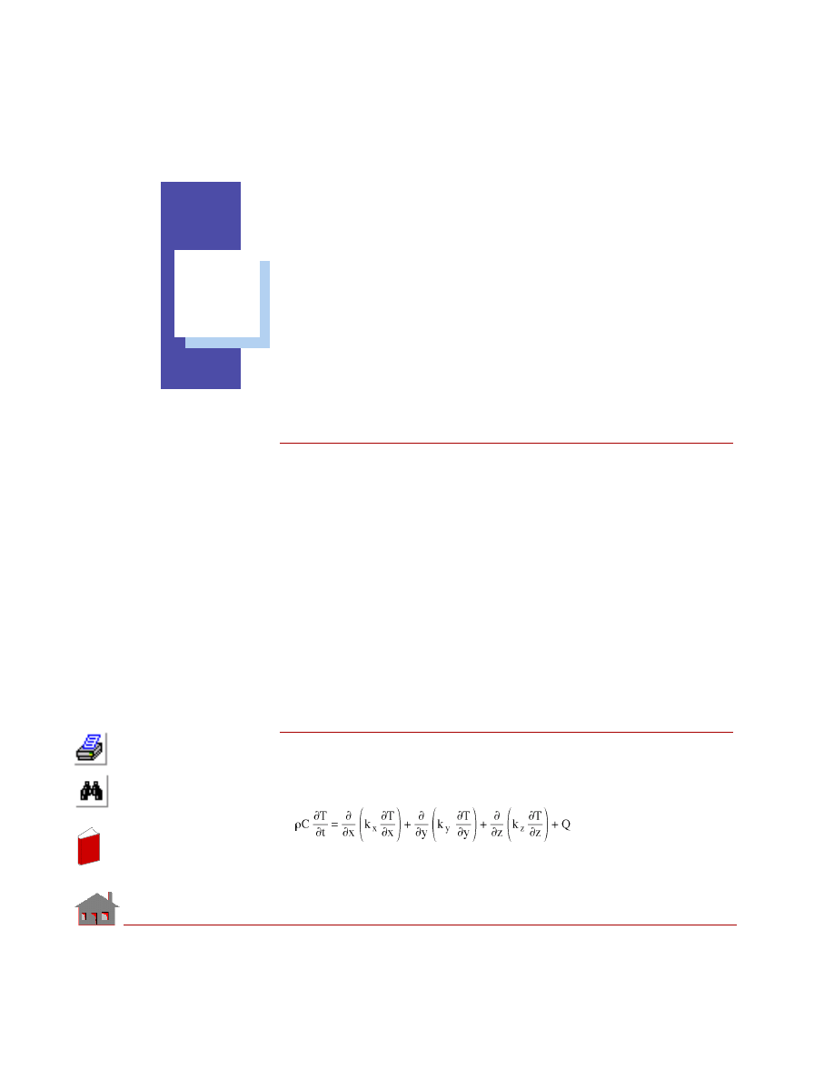
The governing equation for conduction heat transfer is as follows.
(EQ 1-1)
In
de
x
In
de
x

Chapter 1 Introduction
1-2
COSMOSM Advanced Modules
where,
T
= Temperature
t =
Time
ρ
= Density
C
= Specific heat
Q
= Volumetric heat generation rate
k
x
, k
y
, k
z
= Thermal conductivities in global X, Y and Z directions,
respectively
Boundary Conditions
Following boundary conditions can be associated with the heat conduction
equation.
Specified Temperature
Temperature can be prescribed on a part of, or on the whole, boundary of the finite
element domain.
Convection
Heat flux = q = h
c
(T - T
∞
)
(EQ 1-2)
h
c
= Heat transfer coefficient
T
= Surface temperature
T
∞
= Ambient temperature
Radiation
Heat flux = q =
σ ε (T
4
- T
∞
4
)
(EQ 1-3)
σ
= Stefan-Boltzmann constant
ε
= Emissivity
In
de
x
In
de
x
COSMOSM Advanced Modules
1-3
Part 1 HSTAR Heat Transfer Analysis
T
= Surface temperature
T
∞
= Ambient temperature
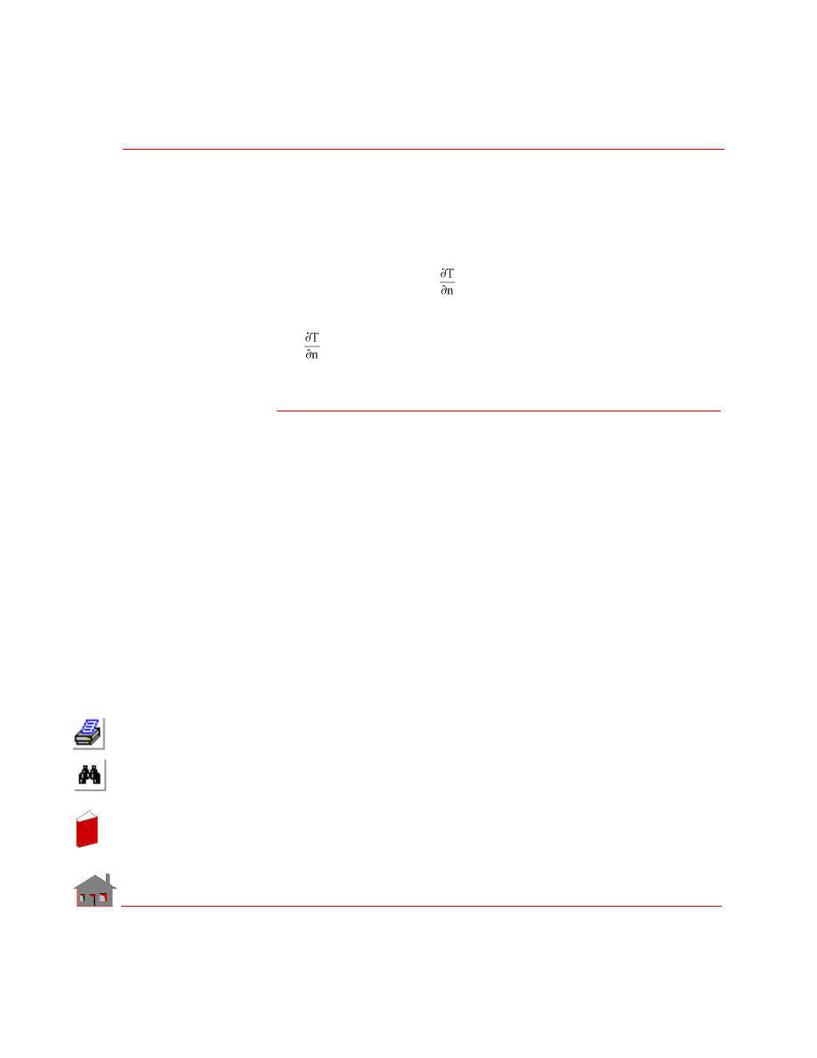
Applied Heat Flux
q = Applied heat flux = - K
(EQ 1-4)
K
= Thermal conductivity
= Normal temperature gradient
Method of Solution
The governing equation along with the specified boundary conditions can be solved
using various solution methods. Some of the solution methods commonly used are
finite difference and finite element method. Finite element method is more popular
because of its ability to handle complicated geometry and the ease with which
boundary conditions can be implemented. HSTAR program is based on finite
element method.
In
de
x
In
de
x

1-4
COSMOSM Advanced Modules
In
de
x
In
de
x

COSMOSM Advanced Modules
2-1
2
Analysis
Introduction
The following types of analysis can be performed using HSTAR.
•
Steady state
•
Transient
Steady State Analysis
Steady state implies that temperature at any given point in the medium is constant
with time. In the steady state analysis, the only material property that is needed is the
thermal conductivity.
Transient Analysis
Transient analysis implies that temperature at any given point in the medium varies
with time. In the transient analysis, in addition to thermal conductivity, we also need
to specify density and specific heat of the material. Whether we consider steady state
or transient analysis, nonlinearity comes into picture, when any one of the following
conditions is encountered.
•
Temperature dependent material properties
•
Temperature dependent convection coefficient
In
de
x
In
de
x

Chapter 2 Analysis
2-2
COSMOSM Advanced Modules
•
Temperature dependent heat generation rate
•
Radiation boundary condition
Radiation View Factor Calculation
The Heat Transfer module (HSTAR) has the capability to perform Radiation View
factor calculation for 2D, 3D, and Axisymmetric models. The process requires the
definition of a set of radiation source entities along with a pattern of target entities.
It is also possible to specify a pattern of blocking entities. Blocking geometric
entities stand between the source and target entities and reduce the view factor. The
view factors are calculated between each element associated with the source entity
and each element associated with the pattern of target entities. If blocking is to be
considered, it is necessary to first define the set involving the source and target
entities with the blocking option activated. Next a pattern of blocking entities is
specified independently. For 2D and Axisymmetric models, the target and blocking
entities must be curves, while for 3D models, they can be surfaces or regions. For
more details, refer to the
RVFTYP
and
RVFDEF
(Analysis > Heat_Transfer >
RVF
Entity Type
and
RVF Source/Target
) commands.
An adaptive view factor calculation option has also been implemented for 3D
models. The program will calculate the view factor starting from 4 divisions for
each radiation element, and will continue to increase the number of divisions until
the computed error is within the user specified tolerance or the number of divisions
reaches the maximum allowed which is (20). It is noted that the adaptive
calculation method basically corresponds to the adjustment in the number of
divisions required for numerical integration. Refer to the
RVFTYP
(Analysis >
Heat_Transfer >
RVF Entity Type
) command for details.
Thermo-Electric Coupling
The electric current flow in a conducting medium can produce a considerable
amount of heat and this effect is known as Joule heating. HSTAR considers the
coupling of the electrical and thermal conduction in which the heat generated due to
the current flow along with other specified boundary conditions is used to calculate
the temperature distribution. When thermo-electric coupling is considered, we also
need to specify the electrical conductivity of the material. At present, only steady
state analysis is available.
In
de
x
In
de
x

COSMOSM Advanced Modules
Part 1 HSTAR Heat Transfer Analysis
Loads and Boundary Conditions
The following thermal boundary conditions and loads are considered in HSTAR.
Prescribed Temperature
Temperature on a part or whole of the boundary of the model is specified.
Convection
When a solid is thermally interacting with its surrounding fluid, heat transfer takes
place through the convection process in which the motion of the surrounding fluid
contributes to the thermal exchange between the solid and the fluid. The boundary
condition is applied by specifying the heat transfer coefficient and the ambient
temperature of the surrounding fluid.
Radiation
Generally, heat transfer by radiation becomes significant at high temperatures. The
analysis handles radiation between a surface and ambient atmosphere. The user may
also specify radiation exchange between bodies.
Applied Heat Flux
Heat flux entering a surface can be prescribed as a boundary condition. This is
equivalent to specifying temperature gradient at the surface.
Heat Generation
Whereas the above four boundary conditions are applied to a surface heat generation
is applied within the material. Joule heating (in which heat is generated within the
material due to the resistance to current flow) is an example of heat generation. Heat
generation can be prescribed at a node or in an element.
Time and Temperature Curves
Time curves are used to specify the variation of thermal loads and boundary
conditions as function of time. All the thermal boundary conditions and loads
discussed above can vary with time and this variation is specified by defining a time
curve and associating this curve with the corresponding boundary condition or load.
Temperature curves are used to specify the variation of material properties with
temperature and they are also used to prescribe the variation of heat transfer
coefficient, heat generation rate and surface emissivity with temperature.
In
de
x
In
de
x
Chapter 2 Analysis
2-4
COSMOSM Advanced Modules
Thermal Stress Analysis
Once a thermal analysis is completed, resulting temperature distribution can be used
to calculate thermal stresses in the material. It is now possible to transfer temperature
results from transient analysis solution steps as thermal loading to static analysis (up
to a maximum of 50 steps).
Thermal Bonding
The thermal bonding feature allows the user to connect finite element meshes
without having to preserve the element type compatibility or mesh continuity at the
interface. The geometric entities and corresponding element groups that can be
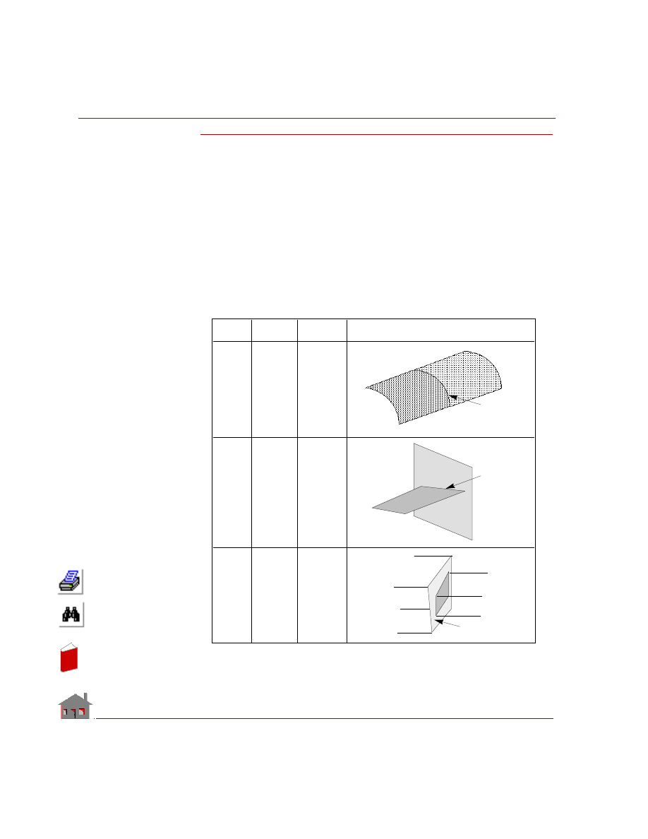
bonded together are shown in the Table 2-1.
Table 2-1. Geometric Connections for Using Bond
Primary or
secondary
Primary or
secondary
Bonding
interface
Primary
Seconda
ry
Bonding
interface
Primary or
secondary
Primary or
secondary
Bonding
interface
E xample
P rimary
E ntity
S e condary
E ntity
To
Conne ct . . .
CR
CR
PLANE2D to
PLANE2D, or
SHELL to
SHELL
CR
SF or RG
SHELL to
SHELL, or
SHELL to
SOLID
SF or RG
SF or RG
SOLID to
SOLID
In
de
x
In
de
x

COSMOSM Advanced Modules
Part 1 HSTAR Heat Transfer Analysis
Bonding of Meshes with Noncompatible Elements
The bond feature allows the user to connect finite element meshes between any two
intersecting geometries without having to preserve the element type compatibility
or mesh continuity at the interface. The geometric entities and corresponding
element groups that can be bonded together are shown in Table 2-1.
In the above table, SHELL refers to all 3-node triangular and 4- or 9-node
quadrilateral shell elements that are supported in COSMOSM. Similarly, SOLID
refers to 8- or 20-node hexahedral solid elements as well as 4- or 10-node TETRA
and 4-node TETRA4R solid elements. Some of the typical applications of the bond
command are also shown in the above table.
✍
The bond feature is currently applicable to linear static, nonlinear structural, and
heat transfer analyses only.
The bond capability is specified using the BONDING submenu from LoadsBC >
STRUCTURAL. The
BONDDEF
(LoadsBC > STRUCTURAL > BONDING >
Define Bond
Parameter
) command bonds faces of elements associated with the
selected geometric entities. The user specifies a primary bond entity (curve,
surface, or region) and a pattern of target entities (curves, surfaces, or regions). All
geometric entities must have meshing completed before issuing this command in
order to generate the bond information. Element edges/faces associated with the
primary geometric entity are bonded with edges/faces of the secondary entities. The
command is useful in connecting parts with incompatible mesh at the interface.
The
BONDLIST
(LoadsBC > STRUCTURAL > BONDING >
List
) command can
be used to list a pattern of bond sets previously defined by the
BONDDEF
(LoadsBC > STRUCTURAL > BONDING >
Define Bond Parameter
) command.
A typical listing is as follows:
Stype
Source
Ttype
#Target
Targets
CR
53
SF
1
7
CR
50
SF
1
7
CR
47
SF
1
7
CR
44
SF
1
7
CR
41
SF
1
7
In
de
x
In
de
x
Chapter 2 Analysis
2-6
COSMOSM Advanced Modules
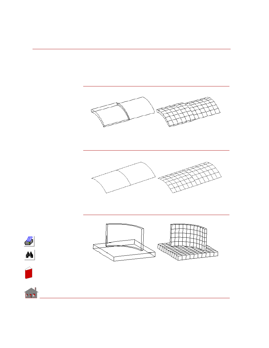
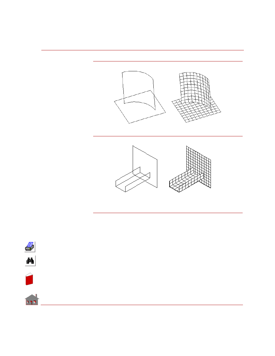
Examples of Bond Connections
The following figures show examples of non-compatible connections where
bonding is useful.
Figure 2-1a. Solid-to-Shell Connection
Figure 2-1b. Shell-to-Shell Connection
Figure 2-1c. Solid-to-Solid Connection
In
de
x
In
de
x
COSMOSM Advanced Modules
Part 1 HSTAR Heat Transfer Analysis
Figure 2-1d. Shell-to-Shell Connection
Figure 2-1e. Shell-to-Shell Connection
Guidelines for Using the Bond Capability
The following points should be considered in the application of this command:
•
The
BONDDEF
(LoadsBC > STRUCTURAL > BONDING >
Define Bond
Parameter
) command internally uses constraint equations to match the dis-
placements and rotations of the two parts. The quality assurance tests have
shown that for parts with reasonable stiffness properties and mesh densities, the
maximum displacement and stress values obtained from the bond command are
within ten percent of those values obtained from a merged model with compati-
ble elements and coincident nodes.
In
de
x
In
de
x
Chapter 2 Analysis
2-8
COSMOSM Advanced Modules
•
The above command is currently applicable to linear static analysis, buckling,
natural frequency computations, heat transfer analysis, and nonlinear structural
analysis only.
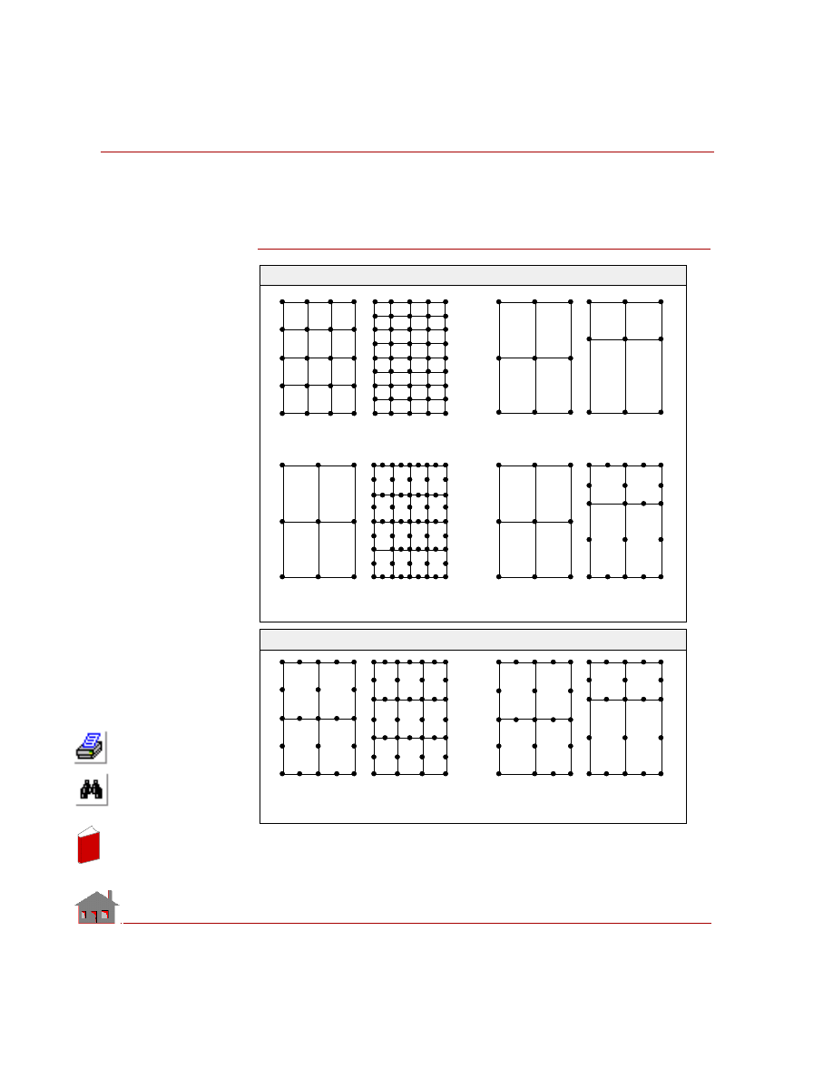
Figure 2-2. Uni-directional and Bi-directional Bonding
Primary or the
source entity is
always the one
that has fewer
degrees of
freedom
For both types
of bonding:
•
Secondary or
the target
entity is
always the
one that has
larger number
of degrees of
•
Source
Target
Source or Target
Target or Source
(Same Element Type)
(Same Element Type)
Unidire c t iona l
Source
Target
Source or Target
Target or Source
(Same Element Type)
Source
Target
Source
Target
(Same Element Type)
Source
Target
Bidire c t iona l
Unidire c t iona l
Source
Target
(Same Element Type)
(Same Element Type)
Source
Target
Source
Target
(Same Element Type)
(Same Element Type)
Bidire c t iona l
In
de
x
In
de
x
COSMOSM Advanced Modules
Part 1 HSTAR Heat Transfer Analysis
•
The
BONDDEF
(LoadsBC > STRUCTURAL > BONDING >
Define Bond
Parameter
) command offers the option of choosing between uni-directional
bond (i.e. connecting all the nodes on primary entity to the elements on the sec-
ondary entity) or bi-directional bond (i.e. connecting the nodes on each entity to
the elements on the other entity). The one directional bond should be used when
connecting lower order elements of the primary (source) entity to lower or
higher order elements of the secondary (target) entity. The bi-directional bond
should be used in connecting higher order elements of the primary entity to
higher order elements of the secondary entity. The following figure illustrates
uni-directional and bi-directional bonding.
•
When bonding solids and shells, it is advisable to use shells as the source and
solids as the target irrespective of the element order.
•
When shell elements are connected to solid elements, the common nodes at the
boundary should
not
be merged as this will free the rational degrees of shell at
that node. Actually, it is advantageous
not
to have coincident nodes at all in
such problems. In shell to shell, or, solid to solid connections, merging of the
coincident nodes at the boundary is allowed.
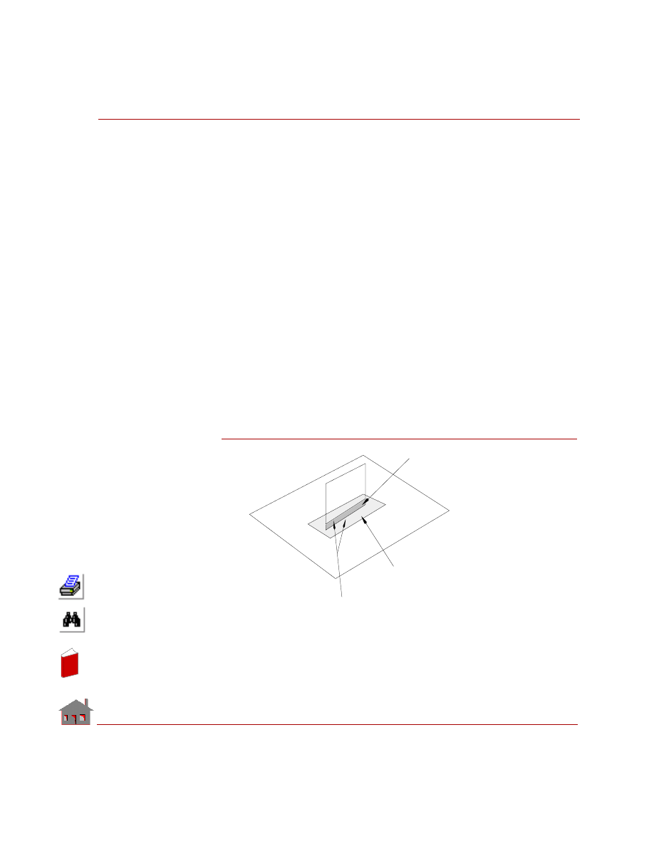
•
In problems where the stress concentration at the bonded intersection is critical,
both parts should have a fine mesh in this region, even though the two meshes
are not matching (see figure below). You may first perform an analysis with
coarse mesh to determine the area requiring fine mesh.
Figure 2-3
Bonding surface. Use fine mesh in this area
based on results from a coarse one.
Replace the gap by a surface or a region
type entity and fill with a fine mesh.
To
p plat
e
Bo
tto
m p
lat
e
Bonding curves
In
de
x
In
de
x

Chapter 2 Analysis
2-10
COSMOSM Advanced Modules
•
The results obtained from the
BONDDEF
(LoadsBC > STRUCTURAL >
BONDING >
Define Bond Parameter
) command may deteriorate in problems
where a rigid part is connected to a relatively flexible part. The bonded area in
the flexible part undergoes warping or has high displacement gradients. The
results will improve if the mesh density for the flexible part is increased in the
bonded area.
•
The actual constraint relations between the nodes of source and target geometric
entities are formed and computed in the analysis stage.
Phase Change
When a material changes its phase from/to solid, liquid, or gas, it either generates
or absorbs heat. The heat associated with phase change is called latent heat.
HSTAR supports phase change by associating the material property enthalpy with a
temperature curve, with a sudden rise or drop at the temperature of phase change.
HSTAR uses this information to calculate and use the latent heat absorbed or
generated by the material.
Thermostat
In transient studies, you can control heat power and heat flux conditions by defin-
ing a thermostat. The thermostat is defined by a sensor location (node), a tempera-
ture range (cut-in and cut-out temperatures), and a temperature curve to determine
the associated heat generation/dissipation boundary conditions.
The thermostat is considered a heater if the cut-in temperature is lower than the cut-
out temperature and a cooler if the cut-in temperature is higher than the cut-out
temperature regardless of the associated boundary conditions.
Before starting a solution step, the program checks the temperature of the sensor. If
the thermostat is a heater, the thermostat is turned on during the next solution step if
the temperature of the node at the sensor is lower than the cut-out temperature and
the device is generating heat. If the thermostat is a cooler, the thermostat is turned
on during the next solution step if the temperature of the node at the sensor is higher
than the cut-out temperature and the device is dissipating heat.
Refer to the THSTAT (LoadsBC, THERMAL, THERMOSTAT, Define) com-
mand for details.
In
de
x
In
de
x

COSMOSM Advanced Modules
3-1
3
Description of Elements
Introduction
The table on the next page lists the elements supported by the HSTAR module.
In
de
x
In
de
x

Chapter 3 Description of Elements
3-2
COSMOSM Advanced Modules
Table 3-1. Elements for Thermal Analysis (HSTAR)
We can also broadly categorize the elements based on the dimensionality of the
problem. TRUSS2D, TRUSS3D, BEAM2D, and BEAM3D elements are used for
one dimensional analysis. PLANE2D, TRIANG, SHELL3T, SHELL4T, SHELL3,
SHELL4, and HLINK are used for two dimensional problems. SOLID, SOLIDL,
TETRA4 and TETRA10 are used for three dimensional problems. CLINK and
RLINK elements could be used for any type of problem. SHELL4L is used for
analyzing layered composite materials.
For a detailed description of all the above elements, refer to the Element Library
chapter in the COSMOSM User’s Guide.
Element Type
Element
Name
2D Spar/Truss
TRUSS2D
2D Elastic Beam
BEAM2D
3D Elastic Beam
BEAM3D
3D Spar/Truss
TRUSS3D
General Mass Element
MASS
Radiation Link
RLINK
Convection Link
CLINK
2D 4- to 8-node Plane Stress, Strain, Body of Revolution
PLANE2D
3D 3- to 6-node Plane Stress, Strain, Body of Revolution
TRIANG
Triangular Thick Shell
SHELL3T
Quadrilateral Thick Shell
SHELL4T
6-Node Triangular Thin Shell
SHELL6
6-Node Triangular Thick Shell
SHELL6T
3D 8- to 20-node Continuum Brick
SOLID
8-node Composite Solid
SOLIDL
3D 4-node Tetrahedron Solid
TETRA4
3D 4-node Tetrahedron Solid with Rotation
TETRA4R
3D 10-node Tetrahedron Solid
TETRA10
Quadrilateral Composite Plate and Shell
SHELL4L
Triangular Thin Shell
SHELL3
Quadrilateral Thin Shell
SHELL4
4-node Hydraulic Link Element
HLINK
Thermal-Fluid Element
FLUIDT
In
de
x
In
de
x

COSMOSM Advanced Modules
3-3
Chapter 3 Description of Elements
In
de
x
In
de
x

Chapter 3 Description of Elements
3-4
COSMOSM Advanced Modules
In
de
x
In
de
x

COSMOSM Advanced Modules
4-1
4
Brief Description
of Commands
Command Summary
Solving a typical thermal problem using finite element method involves generating
a proper finite element mesh, imposing initial and boundary conditions and running
the analysis. The following sections give a brief description of commands that are
used in prescribing boundary conditions, specifying analysis options and solution
parameters. Commands used for a typical 2D analysis are described and similar
commands are available for 3D analysis.
Material Properties
For a steady state analysis we need only to specify thermal conductivity and for a
transient analysis, in addition to thermal conductivity we also need to define
density and specific heat. For thermo-electric coupling, it is also necessary to define
the value of electrical conductivity. All the material properties are defined using
MPROP
(Propsets >
Material Property
) command from the Propsets menu.
Loads and Boundary Conditions
Nodal temperatures at individual nodes and all nodes associated with a curve,
contour, region, surface and volume are defined using the LoadsBC > THERMAL
> TEMPERATURE menu. Convection film coefficients and the associated ambient
temperatures are specified using the LoadsBC > THERMAL > CONVECTION
In
de
x
In
de
x

Chapter 4 Brief Description of Commands
4-2
COSMOSM Advanced Modules
submenu. Radiation energy exchange between a surface and the ambient
atmosphere is specified using the LoadsBC > THERMAL > RADIATION menu.
Heat flux entering or leaving a surface can be prescribed using LoadsBC >
THERMAL > HEAT FLUX menu. Heat generation can be specified at point or
volumetric sources. Nodal heat generation is specified using the LoadsBC >
THERMAL > NODAL HEAT menu. Element heat generation is specified using the
LoadsBC > THERMAL > ELEMENT HEAT menu. For modeling heat transfer due
to flow in a pipe, the HLINK element can be used and the input for thermal
boundary conditions is specified using LoadsBC > THERMAL > HYDRAULIC
FLOW menu.
For radiation heat exchange between multiple bodies, the view factors are
automatically calculated by the program using the following commands from
Analysis > HEAT TRANSFER menu:
RVF Entity Type (RVFTYP)
,
RVF Source/
Target (RVFDEF)
,
Del Rad View Factor (RVFDEL)
and
List Rad View Factor
(RVFLIST)
.
Time and Temperature Curves
Time curves are used to specify the variation of thermal loads and boundary
conditions as function of time. All the thermal boundary conditions and loads can
vary with time. Temperature curves are used to specify the variation of material
properties with temperature and they are also used to prescribe the variation of heat
transfer coefficient and heat generation rate with temperature.
Using a time or temperature curve involves the following steps.
•
Define time or temperature curve using the
CURDEF
(LoadsBC > FUNCTION
CURVE >
Time/Temp Curve
) command. This curve is automatically activated.
•
Define the entity of interest (boundary condition, load, material property, etc.).
•
Deactivate the curve using
ACTSET
(Control > ACTIVATE >
Set Entity
) com-
mand so that this curve is not inadvertently associated with some other entity
defined later on.
For example, we want to prescribe a time varying temperature boundary condition.
First issue
CURDEF
(LoadsBC > FUNCTION CURVE >
Time/Temp Curve
)
command to define time curve. Next, define the nodal temperature at the beginning
of the curve. Deactivate the curve association after you have finished the time-
dependent input.
In
de
x
In
de
x

COSMOSM Advanced Modules
4-3
Part 1 HSTAR Heat Transfer Analysis
Geo Panel: LoadsBC > THERMAL > TEMPERATURE >
Define Nodes (NTND)
Define nodal temperatures ...
Geo Panel: Control > ACTIVATE >
Set Entity (ACTSET)
Set label >
TC: Time Curve
Time curve label >
0
An example of the use of a temperature curve for prescribing a material property
variation is (after defining the temperature curve):
Geo Panel: Propsets >
Material Property (MPROP)
Define thermal conductivity (kx) ...
Geo Panel: Control > ACTIVATE >
Set Entity (ACTSET)
Set label >
TC: Temperature Curve
Temperature curve label >
0
Thermal Stress Analysis
Once a thermal analysis is completed, resulting temperature distribution can be
used to calculate thermal stresses in the material. The following steps can be used
to calculate thermal stresses.
•
Complete the thermal analysis.
•
Use
TEMPREAD
(LoadsBC > LOAD OPTIONS >
Read Temp as Load
) com-
mand to specify the time step at which thermal stress analysis is to be done.
•
Activate the thermal loading using the
A_STATIC
(Analysis > STATIC >
Static
Analysis Options
) command.
•
Run the static analysis using R_STATIC (Analysis > STATIC >
Run Static
Analysis
) command.
Thermal Bonding
The bonding feature can be used to handle problems in which adjacent geometric
entities (as curves, surfaces or regions or combinations of these) are meshed in an
incompatible manner. The
BONDDEF
(LoadsBC > STRUCTURAL > BONDING
>
Define Bond Parameter
) command is used to specify the interfaces along which
mesh incompatibility exists.
In
de
x
In
de
x

Chapter 4 Brief Description of Commands
4-4
COSMOSM Advanced Modules
Thermal Analysis Options
HSTAR is capable of solving both steady state and transient problems. The type of
analysis (steady state or transient) is set using the
A_THERMAL
(Analysis > HEAT
TRANSFER >
Thermal Analysis Options
) command. By default, steady state
analysis is performed.
A_THERMAL
(Analysis > HEAT TRANSFER>
Thermal
Analysis Options
) command also specifies convergence parameters for nonlinear
problems and analysis options for thermo-electric coupling. For transient problems,
the total solution time and time step are prescribed using the
TIMES
(LoadsBC >
LOAD OPTIONS >
Time Parameter
) command. Initial distribution of temperature
is input by the
INITIAL
(LoadsBC > LOAD OPTIONS >
Initial Cond
) command.
The printing and plotting of output results from a transient analysis is controlled by
the
HT_OUT
(Analysis > HEAT TRANSFER >
Thermal Output Options
)
command.
Postprocessing
The output generated by the thermal analysis can be viewed graphically in
GEOSTAR. Issue the Results > PLOT >
Thermal
command to load temperature,
gradient or heat flux values into memory and plot the loaded data. We can also look
at the time history of temperature, gradient, etc. at any node. First issue the
ACTXYPOST
(Display > XY PLOTS >
Activate Post-Proc
) to load proper data
into memory and then issue
XYPLOT
(Display > XY PLOTS >
Plot Curves
) to plot
the time history.
Commands Likely to be Used for a Given Analysis
The following section gives a brief description of commands that may be necessary
to run a given type of analysis once a proper finite element mesh is generated. This
is intended as a general guideline only because the problem at hand may not need
all the commands that are mentioned below or it may need some other commands
which are not mentioned. The commands are given for a typical 2D problem and
similar commands are available for 3D problems.
In
de
x
In
de
x

COSMOSM Advanced Modules
4-5
Part 1 HSTAR Heat Transfer Analysis
Steady State Analysis
Command (Cryptic)
Intended Use
MPROP
(Propsets > Material Property)
Specify material properties
RCONST
(Propsets > Real Constant)
Specify real constants
NTCR
(LoadsBC > THERMAL > TEMPERATURE >
Define Curves)
Specify nodal temperature
boundary conditions
CECR
(LoadsBC > THERMAL > CONVECTION >
Define Curves)
Specify convection boundary
conditions
QESF
(LoadsBC > THERMAL > ELEMENT HEAT
> Define Surfaces)
Specify element heat
generation rate
QSF
(LoadsBC > THERMAL > NODAL HEAT >
Define Surfaces)
Specify nodal heat
generation rate
HFND
(LoadsBC > THERMAL > HEAT FLUX >
Define Nodes)
Specify nodal fluid flow rate
(for HLINK element)
NPRND
(LoadsBC > FLUID FLOW > PRESSURE >
Define Nodes)
Specify nodal pressure
(for HLINK element)
HXCR
(LoadsBC > THERMAL > HEAT FLUX >
Define Curves)
Specify heat flux boundary
condition
RECR
(LoadsBC > THERMAL > RADIATION >
Define Curves)
Specify radiation boundary
condition
RVFTYP
(Analysis > HEAT TRANSFER >
RVF Entity Type)
Specify analysis options for
thermal radiation exchange
RVFDEF
(Analysis > HEAT TRANSFER >
RVF Source/Target)
Specify radiation exchange
between bodies
In
de
x
In
de
x

Chapter 4 Brief Description of Commands
4-6
COSMOSM Advanced Modules
Transient Analysis
In addition to the above commands for a steady state problem, it is necessary to
issue the following commands for a transient problem.
CURDEF
(LoadsBC > FUNCTION CURVE >
Time/Temp Curve)
Specify temperature curve
for defining temperature
dependent material properties
BONDDEF
(LoadsBC > STRUCTURAL > BONDING >
Define Bond Parameter)
Define bonding at interfaces of
geometric entities which are
meshed in an incompatible
manner
A_THERMAL
(Analysis > HEAT TRANSFER >
Thermal Analysis Options)
Specify thermal analysis
options
R_THERMAL
(Analysis > HEAT TRANSFER >
Run Thermal Analysis)
Run the analysis
Command (Cryptic)
Intended Use
CURDEF
(LoadsBC > FUNCTION CURVE >
Time/Temp Curve)
Define a time curve which
specifies the time variation of
loads and boundary conditions
TIMES
(LoadsBC > LOAD OPTIONS > Time
Parameter)
Specify the total solution time
and time step
INITIAL
(LoadsBC > LOAD OPTIONS > Initial Cond)
Specify the initial temperature
distribution
HT_OUTPUT
(Analysis > HEAT TRANSFER >
Thermal Output Options)
Specify printing and plotting
intervals for the results from
thermal analysis
Command (Cryptic)
Intended Use
In
de
x
In
de
x
COSMOSM Advanced Modules
5-1
5
Detailed Examples
Introduction
This example is a typical heat transfer analysis problem solved by the HSTAR
module of COSMOSM through GEOSTAR. A detailed description of the required
steps to set up and solve the problem is furnished.
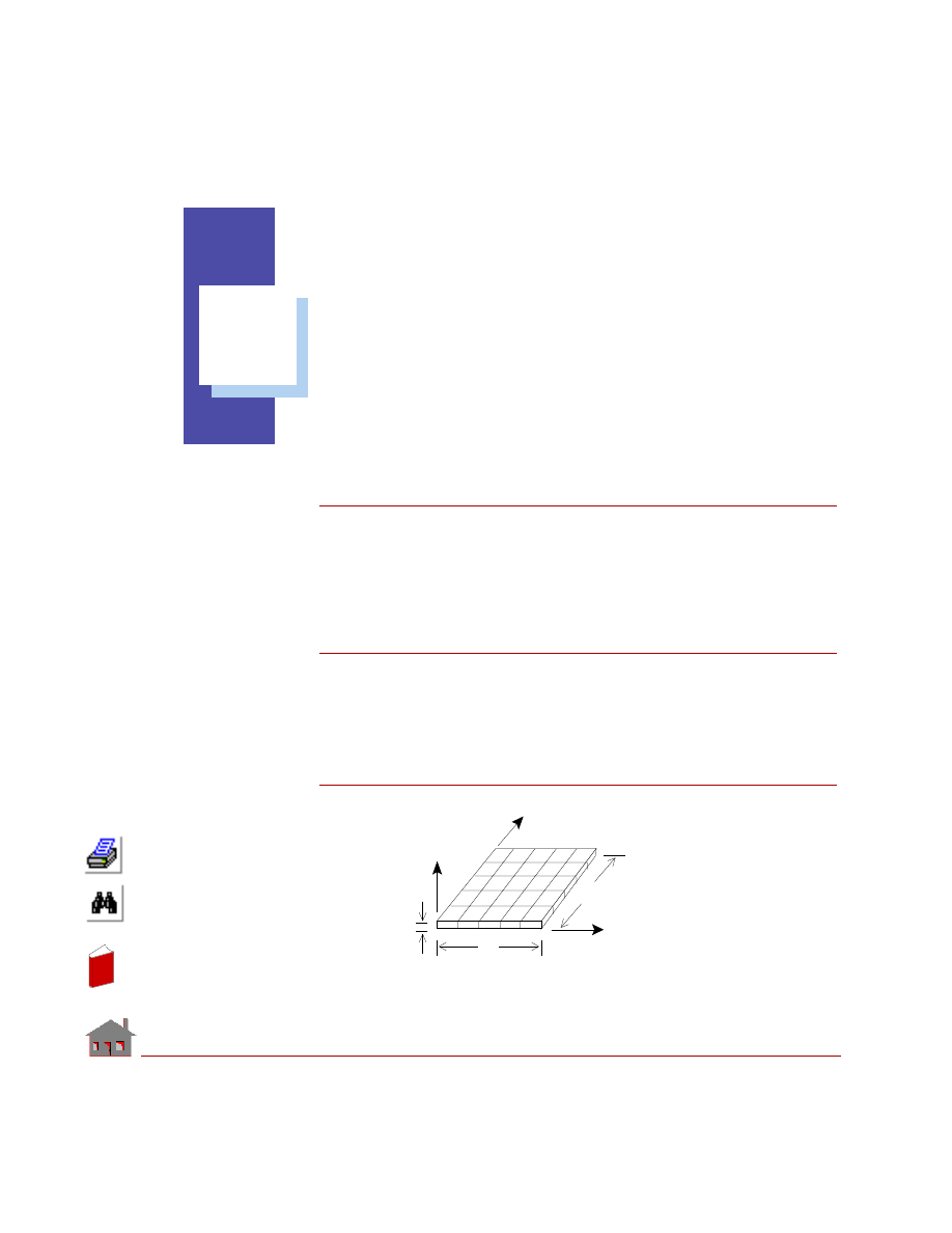
Temperature Distribution on a Plate
Determine the temperature distribution in a plate subjected to temperature and
convection boundary conditions. Consider the effect of constant heat generation on
the plate. The plate is shown in Figure 5-1.
Figure 5-1
h = 0.0001 BTU
X
Y
Z
A
B
C
a
a
h
2
T = 10
°
F
T = 100
°
F
D
/ in - sec -
°
F
In
de
x
In
de
x

Chapter 5 Detailed Examples
5-2
COSMOSM Advanced Modules
Given
Thickness of plate
= h = 1 in
Side of plate
= a = 10 in
Temperature on edge AB
= 100
° F
Ambient temperature
= 10
° F
Thermal conductivity of steel = 0.0006688 BTU/in sec
°F
Constant heat generation
= 0.001 BTU/in
3
sec
Convective heat transfer
coefficient on the edge DC
= 0.0001 BTU/in
2
sec
°F
GEOSTAR Input
Input the problem step-by-step with GEOSTAR commands and perform thermal
analysis. Node generation commands will not be discussed in detail.
1.
Define the element group. For this example, the 2D plane stress element is
selected.
Geo Panel: Propsets >
Element Group (EGROUP)
Element group >
1
Element category >
Area
Element type (for area) >
PLANE2D
Accept defaults ...
2.
Define the Thickness of the Plane Stress element.
Geo Panel: Propsets >
Real Constant (RCONST)
Associated element group >
1
Real constant set >
1
Start location of the real constants >
1
No. of real constants to be entered >
2
RC1: Thickness >
1
RC2: Material angle (Beta) >
0.0
In
de
x
In
de
x

COSMOSM Advanced Modules
5-3
Part 1 HSTAR Heat Transfer Analysis
3.
Define thermal conductivity.
Geo Panel: Propsets >
Material Property (MPROP)
Material property set >
1
Material property name >
kx
Property value >
0.0006688
Since the material is isotropic, this thermal conductivity value is used by default
in all directions, i.e., K
x
= K
y
= K
z
.
4.
The geometry of the model is created next. Change the view to X-Y using the
viewing icon. Define the X-Y plane on which the surface is created as follows:
Define the xy plane.
Geo Panel: Geometry > GRID >
Plane (PLANE)
Rotation/sweep axis >
Z
Offset on axis >
0.0
Grid line style >
Solid
Geo Panel: Geometry > SURFACES >
Define w/4 Coord (SF4CORD)
Surfaces >
1
XYZ-coordinate value of Keypoint 1>
0,0,0
XYZ-coordinate value of keypoint 2 >
10,0,0
XYZ-coordinate value of keypoint 3 >
10,10,0
XYZ-coordinate value of keypoint 4 >
0,10,0
5.
Define elements and nodes through mesh generation.
Geo Panel: Meshing > PARAMETRIC MESH >
Surfaces (M_SF)
Beginning surface >
1
Ending surface >
1
Increment >
1
Number of nodes per element >
4
Number of elements on 1st curve >
5
Number of elements on 2nd curve >
5
Spacing ratio for 1st curve >
1.0
Spacing ratio for 2nd curve >
1.0
In
de
x
In
de
x

Chapter 5 Detailed Examples
5-4
COSMOSM Advanced Modules
6.
See the Auto scale icon to properly view the model. Define temperature bound-
ary conditions along curve 3.
Geo Panel: LoadsBC > THERMAL > TEMPERATURE >
Define Curves (NTCR)
Beginning curve >
3
Value >
100
Ending curve >
3
Increment >
1
7.
Define convection boundary conditions along curve 4.
Geo Panel: LoadsBC > THERMAL > CONVECTION >
Define Curves (CECR)
Beginning curve >
4
Convection coefficient >
0.0001
Ambient temperature >
10
Ending curve >
4
Increment >
1
Time curve for ambient temperature >
0
8.
The constant heat generation rate is specified using the
QESF
(LoadsBC >
THERMAL > ELEMENT HEAT >
Define Surfaces
) command.
Geo Panel: LoadsBC > THERMAL > ELEMENT HEAT >
Define Surfaces
(QESF)
Beginning surface >
1
Value >
0.001
Ending surface >
1
Increment >
1
9.
The thermal analysis option by default is “steady state” thus the
A_THERMAL
(Analysis > HEAT TRANSFER >
Thermal Analysis Options
) command is not
required. Just use the
R_THERMAL
(Analysis > HEAT TRANSFER >
Run
Ther-
mal Analysis
) command to run the heat transfer program.
When the analysis is completed, the program will return to GEOSTAR. Next use
the
EDIT
(FILE >
Edit a File
) command or your favorite editor to view the output file
(*.TEM). Use the
ACTTEMP
and
TEMPPLOT
(Results > PLOT >
Thermal
) commands
to generate a temperature contour plot.
In
de
x
In
de
x
COSMOSM Advanced Modules
5-5
Part 1 HSTAR Heat Transfer Analysis
Results
Temperature at node 24:
Analytical solution
= 76.0306
° F
HSTAR solution
= 76.0307
° F
An Example of Thermal Bonding
The following example illustrates the use of the BONDING feature in thermal
analysis. The problem is to find the temperature distribution in a plate which is
subjected to temperature boundary conditions. To illustrate the bonding capability
of the HSTAR program, the plate is divided into two surfaces which are meshed in
such a way that the meshing is incompatible at the interface of the two surfaces.
Figure 5-2
Given
Thickness of the plate
= 1 cm
Length of the plate
= l = 2 m
Width of the plate
= 1 m
Temperature on edge AB = 0
° C
Temperature on edge CD = 100
° C
Thermal conductivity
of the material
= 1 W/m - K
b
Node 49
T = 0
°
C
B
A
D
C
T = 100
°
C
X
Y
In
de
x
In
de
x

Chapter 5 Detailed Examples
5-6
COSMOSM Advanced Modules
GEOSTAR Input
The following is a step by step procedure to generate the required input and
perform the thermal analysis.
1.
Define the element group 2D Plane stress element is selected.
Geo Panel: Propsets >
Element Group (EGROUP)
Element group >
1
Element category > Area
Element type (for area) >
PLANE2D
Accept defaults ...
2.
Define the thickness of the Plane stress element through a real constant set.
Geo Panel: Propsets >
Real Constant (RCONST)
Associated element group >
1
Real constant set >
1
Start location of the real constants >
1
No. of real constants to be entered >
2
RC1: Thickness >
0.01
RC2: Material angle (Beta) >
0.0
3.
Define thermal conductivity.
Geo Panel: Propsets >
Material Property (MPROP)
Material property set >
1
Material property name >
kx
Property value >
1.0
4.
Define the geometry of the model. Change the view to X-Y using the Viewing
icon. Define the X-Y plane on which the surface is created as follows:
Geo Panel: Geometry > GRID >
Plane (PLANE)
Rotation/sweep axis >
Z
Offset on axis >
0.0
Grid line style >
Solid
In
de
x
In
de
x

COSMOSM Advanced Modules
5-7
Part 1 HSTAR Heat Transfer Analysis
Geo Panel: Geometry > SURFACES >
Define w/4 Coord (SF4CORD)
Surface > 1
XYZ-coordinate of keypoint 1 >
0,0,0
XYZ-coordinate of keypoint 2 >
1,0,0
XYZ-coordinate of keypoint 3 >
1,1,0
XYZ-coordinate of keypoint 4 >
0,1,0
Generate an additional surface by translating the first surface in the x-direction
by 1 m.
Geo Panel: Geometry > SURFACES > GENERATION MENU >
Generate
(SFGEN)
Generation number >
1
Beginning surface >
1
Ending surface >
1
Increment >
1
Generation flag >
Translation
X-displacement >
1.0
Y-displacement >
0.0
Z-displacement >
0.0
5.
Use the Auto scale option to see the model clearly. Define elements and nodes
through mesh generation. Note that the two surfaces are meshed separately to
create incompatibility at the interface of the two surfaces.
Geo Panel: Meshing > PARAMETRIC MESH >
Surfaces (M_SF)
Beginning surface >
1
Ending surface >
1
Increment >
1
Number of nodes per element >
4
Number of elements on 1st curve >
5
Number of elements on 2nd curve >
5
Accept defaults ...
Geo Panel: Meshing > PARAMETRIC MESH >
Surfaces (M_SF)
Beginning surface >
2
Ending surface >
2
Increment >
1
Number of nodes per element >
4
In
de
x
In
de
x

Chapter 5 Detailed Examples
5-8
COSMOSM Advanced Modules
Number of elements on 1st curve >
5
Number of elements on 2nd curve >
4
Accept defaults ...
6.
Merge the coincident nodes
Geo Panel: Meshing > NODES >
Merge (NMERGE
)
Accept defaults ...
7.
Define temperature boundary conditions along the left and right edges of the
plate.
Geo Panel: LoadsBC > THERMAL > TEMPERATURE >
Define Curves (NTCR)
Beginning curve >
3
Value >
0
Ending curve >
3
Increment >
1
Geo Panel: LoadsBC > THERMAL > TEMPERATURE >
Define Curves (NTCR)
Beginning curve >
5
Value >
100
Ending curve >
5
Increment >
1
8.
Define bonding between the two surfaces
Geo Panel: LoadsBC >STRUCTURAL >BONDING >
Define Bond Parameter
(BONDDEF)
Bonding set >
1
Primary geometric entity type >
Curve
Primary curve >
4
Secondary geometric entity type >
Curve
Beginning curve >
4
Ending curve >
4
Increment >
1
Direction flag >
Bi Dir
In
de
x
In
de
x

COSMOSM Advanced Modules
5-9
Part 1 HSTAR Heat Transfer Analysis
9.
Run the thermal analysis.
Geo Panel: Analysis > HEAT TRANSFER >
Run Thermal Analysis
(R_THERMAL)
After the analysis is completed, the program will return to GEOSTAR. Use the
ACTTEMP
and
TEMPPLOT
(Results > PLOT >
Thermal
) command to generate a
temperature plot.
Results
Temperature at node 49:
Analytical solution
= 50
° C
HSTAR solution
(with bonding)
= 50
° C
HSTAR solution
(without bonding)
= 75.9
° C
Listing of Session File
EGROUP,1,PLANE2D,0,1,0,0,0,0,0,
RCONST,1,1,1,2,0.01,0,
MPROP,1,KX,1.0,
PLANE,Z,0,1,
VIEW,0,0,1,0,
SCALE,0,
SF4CORD,1,0,0,0,1,0,0,1,1,0,0,1,0,
SFGEN,1,1,1,1,0,1.0,0,0,
M_SF,1,1,1,4,5,5,1,1,
M_SF,2,2,1,4,5,4,1,1,
NMERGE,1,66,1,0.0001,0,1,0,
NTCR,3,0.0,3,1,
NTCR,5,100.0,5,1,
BONDDEF,1,0,4,0,4,4,1,2,
R_THERMAL
In
de
x
In
de
x

5-10
COSMOSM Advanced Modules
In
de
x
In
de
x

COSMOSM Advanced Modules
6-1
6
Verification Problems
Introduction
In the following, a comprehensive set of verification problems are provided to
illustrate the various features of the heat transfer analysis module (HSTAR). The
problems are carefully selected to cover a wide range of applications in the field
of thermal analysis.
The input files for the verification problems are available in the “...\Vprobs\
HeatTransfer” folder. Where “...” denotes the COSMOSM installation folder. For
example the input file for problem TL01 is “...\Vprobs\HeatTransfer\TL01.GEO”.
In
de
x
In
de
x

6-2
COSMOSM Advanced Modules
Linear Heat
Transfer Analysis
In
de
x
In
de
x

COSMOSM Advanced Modules
6-3
Part 1 HSTAR Heat Transfer Analysis
TL01: Steady State Heat
Conduction in a Square Plate
TYPE:
Steady state heat conduction with prescribed temperature boundary conditions,
SHELL3T elements are used.
REFERENCE:
Carslaw, H. S., and Jaeger, J. C., “Conduction of Heat in Solids,” 2nd edition,
Oxford
University Press, 1959.
PROBLEM:
Determine the temperature at the center of a square plate with prescribed edge
temperatures.
GIVEN:
Thermal Conductivity
= 43 w/m
°C
Boundary Conditions:
Along the edge AB, temp. = 0
° C
Along the edge BC, temp. = 0
° C
Along the edge CD, temp. = 0
° C
Along the edge DA, temp. = 100
° C
Width and Height of Plate = 4 m
MODELING HINTS:
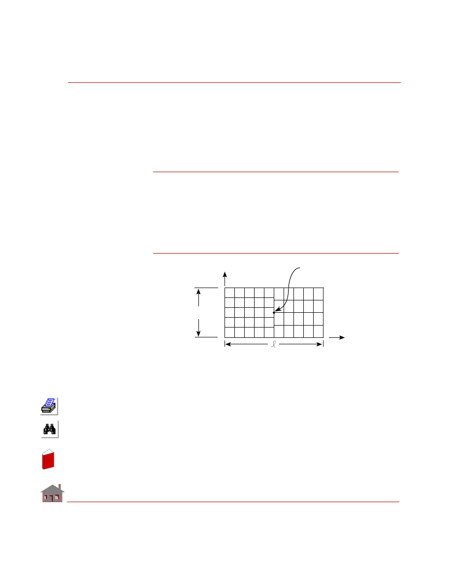
Since the plate and boundary conditions are symmetrical about cross-section I-I,
only one half of the plate is modeled using SHELL3T elements as shown in the
figure.
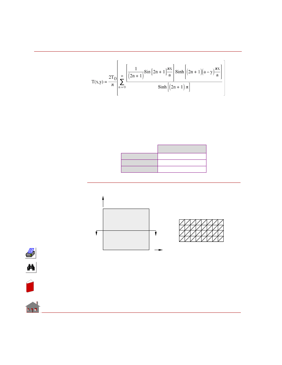
ANALYTICAL SOLUTION:
Temperature at any point (x,y) in the plate is:
In
de
x
In
de
x
Chapter 6 Verification Problems
6-4
COSMOSM Advanced Modules
Where
a
= The length of a side of plate
T
o
= The temperature at x = 0
COMPARISON OF RESULTS:
At the center of the plate (Node 41).
Figure TL01-1
Temperature
°
C
Theory
25
COSMOSM
25
Difference
0%
39
38
40
37
Y
C
D
X
A
B
I
I
0
°
0
°
0
°
100
°
1
2
3
4
5
41
6
42
7
43
8
44
9
45
28
36
19
27
10
18
Problem Sketch
Finite Element Model
In
de
x
In
de
x
COSMOSM Advanced Modules
6-5
Part 1 HSTAR Heat Transfer Analysis
TL02: Steady State Heat Conduction
in an Orthotropic Plate
TYPE:
Steady state heat conduction with convection boundary conditions, SHELL4
elements are used.
REFERENCE:
M. N. Ozisik, “Heat Conduction,” Wiley, New York, 1980.
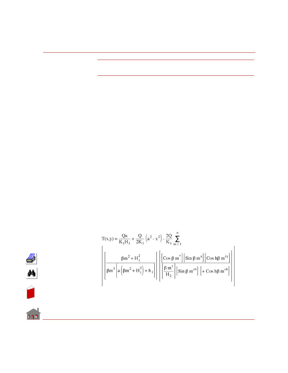
PROBLEM:
Determine the temperature distribution in an orthotropic plate with a constant rate of
heat generation. The boundaries at x = 0 and y = 0 are insulated, and those at x = a
and y = b are dissipating heat by convection into the atmosphere which is at zero
temperature.
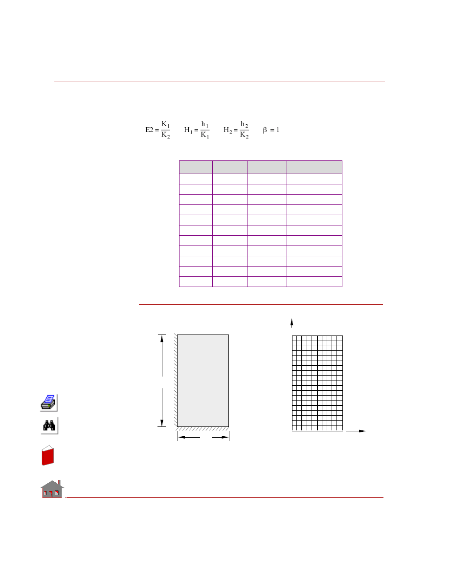
GIVEN:
MODELING HINT:
Plate is modeled using 200 SHELL4 elements.
ANALYTICAL SOLUTION:
Thermal Conductivity
along x direction = K
x
= 10 w/m
° C
along y direction = K
y
= 20 w/m
° C
Length of the plate = a = 1 m
Width of the plate = b = 2 m
Thickness of the plate = 0.1 m
Rate of heat generation Q = 100 w/m
3
Convection Heat Transfer Coefficient
at the boundary BC = h
1
= 10 w/m
2
° C
at the boundary DC = h
2
= 20 w/m
2
° C
In
de
x
In
de
x
Chapter 6 Verification Problems
6-6
COSMOSM Advanced Modules
Where:
K
1
= K K
2
= Ky
COMPARISON OF RESULTS:
Figure TL02-1
Node
X (m)
Theory
COSMOSM
111
0.0
8.5094
8.5122
112
0.1
8.4832
8.4860
113
0.2
8.4045
8.4073
114
0.3
8.2728
8.2757
115
0.4
8.0874
8.0902
116
0.5
7.8471
7.8499
117
0.6
7.5505
7.5533
118
0.7
7.1959
7.1985
119
0.8
6.7811
6.7836
120
0.9
6.3038
6.3060
121
1.0
5.7613
5.7631
b
Insulated
Insulated
a
221
231
1
11
y
x
Problem Sketch
Finite Element Model
A
B
C
D
T = 0
°
C
h = 20 w/m
°
C
2
2
∞
T = 0
°
C
h = 10 w/m
°
C
2
1
∞
In
de
x
In
de
x

COSMOSM Advanced Modules
6-7
Part 1 HSTAR Heat Transfer Analysis
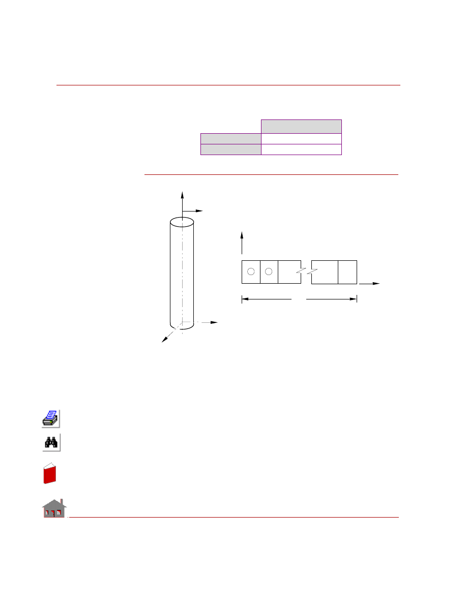
TL03: Transient Heat Conduction
in a Long Cylinder
TYPE:
Transient heat conduction with convection boundary conditions, PLANE2D
elements.
REFERENCE:
J. P. Holman, “Heat Transfer,” McGraw-Hill Book Company, 1976, p. 117.
PROBLEM:
A long aluminum cylinder, 5 cm in diameter and initially at 200
°C, is suddenly
exposed to a convection environment at 70
°C and h = 525 W/m
2
°C. Calculate the
temperature at a radius of 1.25 cm, one minute after the cylinder is exposed to the
environment.
GIVEN:
Radius of cylinder
= r
o
= 0.025 m
Thermal conductivity
= K = 215 W/m
° C
Mass density
=
ρ = 2700 Kg/m
3
Specific heat
= C = 936.8 J / Kg
° C
Initial temperature
= T
0
= 200
° C
Ambient temperature
= T
∞
= 70
° C
Convective heat
transfer coefficient
= h = 525 w/m
2
°C
MODELING HINTS:
Since the cylinder and boundary conditions are axisymmetric, PLANE2D
axisymmetric elements are used to model this problem.
In
de
x
In
de
x
Chapter 6 Verification Problems
6-8
COSMOSM Advanced Modules
COMPARISON OF RESULTS:
Comparison of solutions is made at r = 0.0125 m (node 21) and at t = 60 sec:
Figure TL03-1
Temperature
°
C
Theory
118.40
COSMOSM
119.49
h, T
8
X
Z
Problem
Sketch
r
o
Y
2
6
4
40
42
41
39
1
5
3
Y
Finite Element Model
X
1
2
r
o
In
de
x
In
de
x

COSMOSM Advanced Modules
6-9
Part 1 HSTAR Heat Transfer Analysis
TL04: Thermal Stresses in
a Hollow Cylinder
TYPE:
Thermal stress analysis, PLANE2D axisymmetric element.
REFERENCE:
Timoshenko and Goodier, “Theory of Elasticity,” McGraw-Hill Book Co., New
York, 1961.
PROBLEM:
The hollow cylinder in plane strain is subjected to two independent loading
conditions.
1.
An internal pressure Pa
2.
A steady state axisymmetric temperature distribution due to the following
boundary conditions.
At r = 1, temperature = 100
° F
At r = 2, temperature = 0
° F
Pressure and Temperature Loading PLANE2D Axisymmetric Model.
GIVEN:
E
= 30 x 10
6
psi
a
= 1 in
b
= 2 in
ν
=
0.3
α
x
= 1 *10
-6
/
°F
Kx = 1 Btu/in sec
°F
Pa = 100 psi
T
a
= 100
°F
T
b
= 0
°F
In
de
x
In
de
x
Chapter 6 Verification Problems
6-10
COSMOSM Advanced Modules
COMPARISON OF RESULTS:
Figure TL04-1
Theory
COSMOSM
Temperature in
°
F
Node 23
59.401
59.398
Node 42
23.447
23.447
Stress at r=1.325” (Center of Element 7) in psi
T
r
(SX)
-398.34i
-398.14i
T
θ
(SZ)
-592.47i
-596.38
L
Problem Sketch
T
Pa
Tr
15
14
28
1 2 3
12
45
x
y
b
31
8
7
30
C
Finite Element Model
16
a
θ
In
de
x
In
de
x

COSMOSM Advanced Modules
6-11
Part 1 HSTAR Heat Transfer Analysis
TL05: Heat Conduction Due to
a Series of Heating Cables
TYPE:
Steady state heat conduction due to internal heat generation (PLANE2D elements).
REFERENCE:
J. N. Reddy, “An introduction to the finite element method.” McGraw-Hill Book
Co., 1984, p. 260.
PROBLEM:
A series of heating cables have been placed in a conducting medium as shown in
figure. The medium has conductivities of K
x
= 10 w/cm
°K and K
y
= 15 w/cm
°K.
The Upper surface is exposed to a temperature of -5
° C, and the lower surface is
bounded by an insulating medium. Assuming that each cable is a point source of 250
w, determine the temperature distribution in the medium.
GIVEN:
Thermal conductivity in:
x direction K
x
= 10 w/cm
°K
y direction K
y
= 15 w/cm
°K
Ambient temperature T
= 268
° K
Convection coefficient h
= 5 w/cm
2
°K
Rate of heat generation in the cable per unit length Q= 250 w
MODELING HINTS:
Since the cables are uniformly distributed throughout the medium, the problem can
be simplified by analyzing only the section ABCD as shown in the figure. Because
of symmetry, consider the sides AD and BC to be insulated. Since the medium is
symmetric about x-y plane, plane strain option of PLANE2D elements has been
selected.
In
de
x
In
de
x
Chapter 6 Verification Problems
6-12
COSMOSM Advanced Modules
Figure TL05-1
145
153
1
9
D
C
113
A
B
4
Cables
2
X
4
Y
T = 268
°
K
h = 5 w/cm
°
K
8
2
Insulated
Finite Element
Model
Y
X
Problem Sketch
Cabl
C
D
A
B
In
de
x
In
de
x

COSMOSM Advanced Modules
6-13
Part 1 HSTAR Heat Transfer Analysis
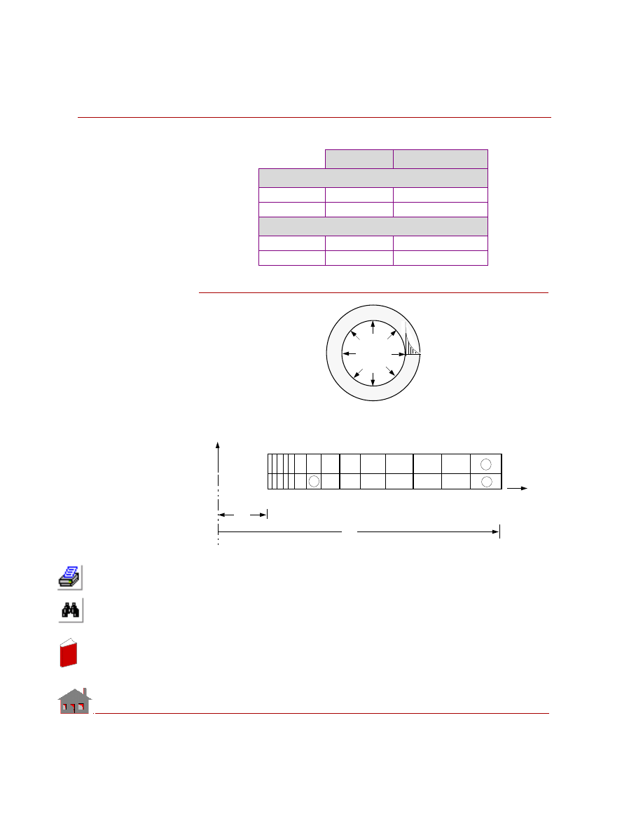
TL06: Pressure Distribution
in an Aquifer Flow
TYPE:
Seepage flow, PLANE2D elements.
REFERENCE:
J. N. Reddy, “An introduction to the finite element method,” McGraw-Hill Book
Co., 1984, p. 103.
PROBLEM:
A well penetrates an aquifer and pumping is done at a rate of Q = 150 m
3
/h. The
permeability of the aquifer is K = 25 m
3
/(hm
2
). The aquifer is unconfined and radial
symmetry exists in the flow field (with the origin of the radial coordinate being at
the pump). A constant head of U = 50 m exists at a radial distance of L = 200 m.
Determine the distribution of piezometric head.
GIVEN:
Permeability of aquifer
= K = 25 m
3
/(h m
2
)
piezometric head (at r = 200 m) = U = 50 m
Rate of pumping
= Q = 150 m
3
/h
MODELING HINTS:
This problem is modeled by PLANE2D elements. Since the distribution of pressure
in the radial direction is a function of logarithm of radial coordinate, variable node
spacing is used to get better results. The ratio of last division size to the first division
size along the radial direction is assumed to be 6. This problem has been solved
using two types of PLANE2D elements.
Case A
Plane strain option of PLANE2D elements has been selected. This type of model is
especially useful to visualized piezometric head contours (which are concentric
circles).
Case B
Axial symmetry of the problem is used to simplify the model. Axisymmetric option
of PLANE2D elements has been selected. Note that the governing equation of this
In
de
x
In
de
x
Chapter 6 Verification Problems
6-14
COSMOSM Advanced Modules
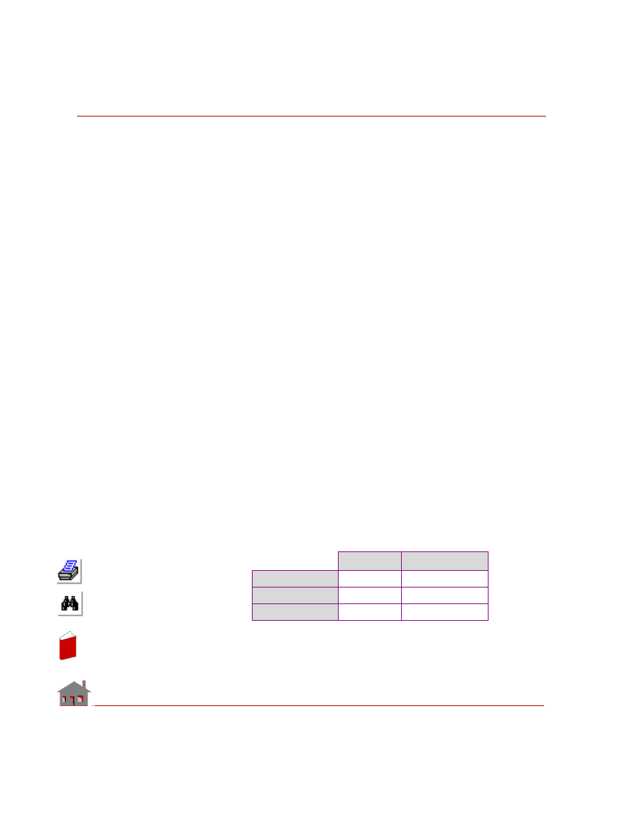
problem is similar to that of steady state heat conduction in radial direction. Hence
this problem has been solved by identifying the variables as shown in Table 6-1
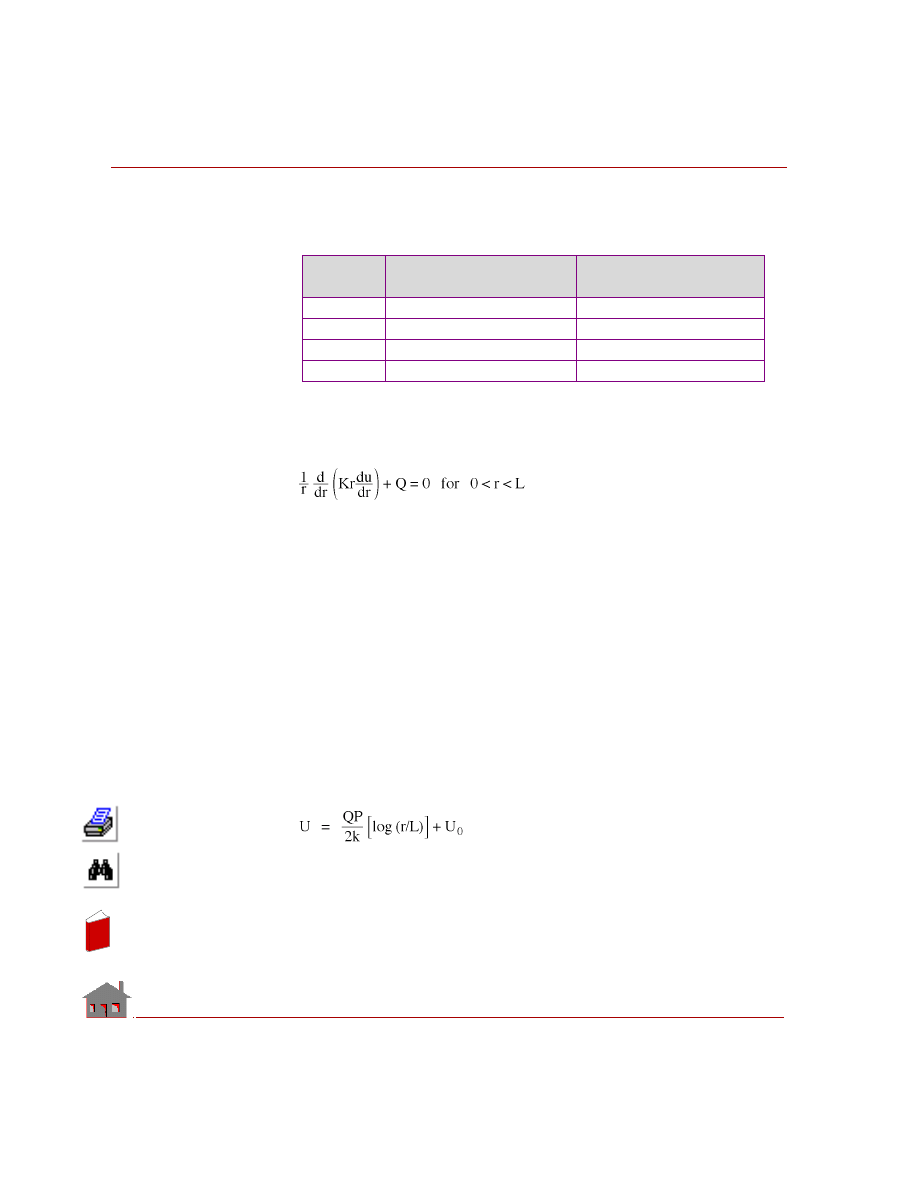
Table TL06-1. Interpretation of Heat Conduction Variables in Seepage Problem
ANALYTICAL SOLUTION:
The governing equation for an unconfined aquifer with flow in the radial direction
is given by:
Where:
r
= radial coordinate
Q = recharge
K = coefficient of permeability
u
= piezometric head
Note that pumping is considered to be a negative recharge.
The associated boundary conditions are at
r
= 0
Q = recharge
r
= L
u
= u
0
Solution of the above differential equation is given by
Variable
Steady State
Heat Conduction
Pressure Distribution
is an Aquifer Flow
u
Temperature
Piezometric head
K
Thermal conductivity
Permeability coefficient
Q
Internal heat generation
Recharge
r
Radial coordinate
Radial coordinate
In
de
x
In
de
x
COSMOSM Advanced Modules
6-15
Part 1 HSTAR Heat Transfer Analysis
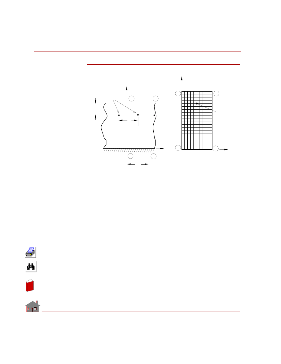
COMPARISON OF RESULTS:
Piezometric head at r = 84.18246 (at Node 5)
Figure TL06-1
Theory
COSMOSM
Case A
COSMOSM
Case B
Head (m)
49.174
49.205
49.750
8 9 10 11 12 13 14
1 2 3 4 5 6 7
25
19
13
7
73
67
61
55
49
43
37
31
6
5
4
Case B
Case A
CL
L
X
Y
CL
X
Problem Sketch and Finite Element Model
Z
L
3
In
de
x
In
de
x
Chapter 6 Verification Problems
6-16
COSMOSM Advanced Modules
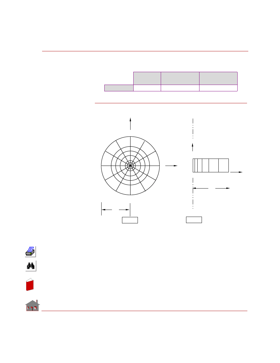
TL07: Potential Flow Over a Cylinder
Confined Between Two Walls
TYPE:
Potential flow: stream function and velocity potential formulations
REFERENCE:
Irving H. Shames, “Mechanics of Fluids,” McGraw-Hill Book Co., 1982.
PROBLEM:
Consider an infinitely long
cylinder at rest in a large
body of fluid flowing
uniformly at right angles
to the axis of the cylinder.
Assuming irrotational and
incompressible flow, find
the maximum velocity of
the flow.
Solve the problem using the
Stream function
formulation.
GIVEN:
Diameter of cylinder
= d = 0.2 m
Velocity = V
0
= 1.0 m/s
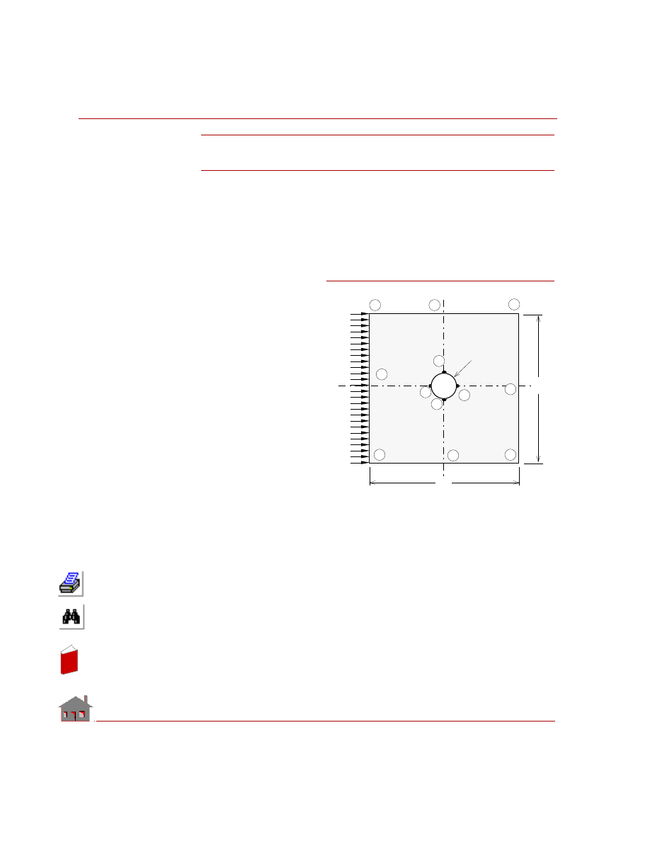
MODELING HINTS:
This problem has been modeled by PLANE2D elements. Note that the model is
symmetric about the axes EG and HF. Hence it is sufficient to analyze one quarter
of the model with the appropriate boundary conditions on the axes of symmetry.
Assume that the velocity is constant at a distance of 1 m from the axis of cylinder.
Since the gradients of stream function are very high near the cylinder, variable mesh
spacing has been selected. Note that the variable finite element mesh can be
generated very easily using mesh generation commands.
V
o
H
0 .1 m
C
d
Problem Sketch
A
E
D
F
B
G
K
J
I
L
d
Figure TL07-1
In
de
x
In
de
x
COSMOSM Advanced Modules
6-17
Part 1 HSTAR Heat Transfer Analysis
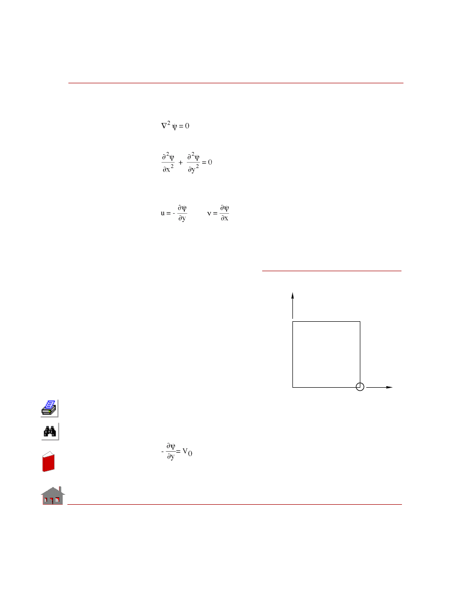
Stream Function Formulation
The incompressible steady flow may be represented by Laplace equation:
For a two dimensional flow, the above equation can be rewritten as:
Where
Ψ is called stream function. The velocity field may be obtained from stream
function as:
Note that the stream function has a property that the flow normal to streamlines is
zero. Hence, the fixed surfaces correspond to streamlines. Thus, the cylindrical
surface IL may be treated as a streamline.
Also, note that the velocity normal
to the horizontal axis of symmetry
is zero. Hence, the horizontal axis
of symmetry may also be treated as
a streamline. Similarly, the top
surface (represented by line DH) is
also a streamline.
Since the velocity field depends
on the relative difference of stream
functions take the value of stream-
line along the horizontal axis of
symmetry as zero,
i.e.,
ψ
EI
-
ψ
IL
= 0
Along the surface ED,
u =V
0
= Velocity of flow
ν = 0
Figure TL07-2
Y
H
D
E
L
ψ
= 1
ψ
= 0
ψ
= 0
I
ψ
= V Y
o
X
Boundary Conditions
In
de
x
In
de
x
Chapter 6 Verification Problems
6-18
COSMOSM Advanced Modules
or
ψ = -V
0
Y
ψ
DH
- = -V
0
Y
and
ψ
DH
- = -1
Analogy between stream function formulation of potential flow and heat
conduction. The governing equation of stream function formulation stream of
potential flow is similar to steady state heat conduction equation with no heat
generation.
•
Head conduction
•
Gradients of temperature
•
Stream function
•
Temperature
•
Potential flow
•
Velocity components
Hence, HSTAR may be used to solve the potential flow problem by following the
steps given below.
1.
Set thermal conductivity Kx = 1.
2.
Apply prescribed temperature boundary conditions wherever prescribed stream
functions are to be applied.
3.
The velocity field may be obtained by calculating the gradients of stream func-
tion (please see the options in
command).
COMPARISON OF RESULTS:
At (x = 0, y = 0.1) (i.e., at Node 861).
Stream Function Formulation
Theory
COSMOSM
Ψ
0
0
u
= − (∂Ψ/∂
y
)
2
1.914
υ = (∂Ψ/∂
x
)
0
0.025
In
de
x
In
de
x
COSMOSM Advanced Modules
6-19
Part 1 HSTAR Heat Transfer Analysis
TL08: Transient Heat Conduction in
a Slab of Constant Thickness
TYPE:
Linear transient heat conduction, TRUSS2D
elements.
REFERENCE:
Gupta, C. P., and Prakash, R., “Engineering Heat
Transfer,” Nem Chand and Bros., India, 1979, pp.
155-157.
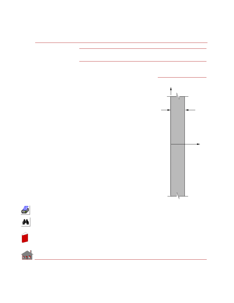
PROBLEM:
A large plate of thickness 62.8 cm is initially at a
temperature of 50
° C. Suddenly, both of its faces
are raised to and held at 550
° C.
Determine:
1.
The Temperature at a plane 15.7 cm from the
left surface, 5 hours after the sudden change in
surface temperature.
2.
Instantaneous heat flow rate at the left surface
at the end of 5 hours.
3.
Total heat flow across the surface at the end of
5 hours.
GIVEN:
Thickness of slab
= L = 0.628 m
Area of cross section
= 1 m
2
Density
=
ρ = 23.2 Kg/m
3
Solution time
= 5 hours
Initial temperature
= T
i
= 50
° C
Thermal conductivity
= K = 46.4 J/m - hr
°K
Specific heat
= c = 1000 J/Kg -
°K
Left and right surface temperatures = T
s
= 550
° C
Figure TL08-1
X
L
y
Problem Sketch
Ts
Ts
In
de
x
In
de
x
Chapter 6 Verification Problems
6-20
COSMOSM Advanced Modules
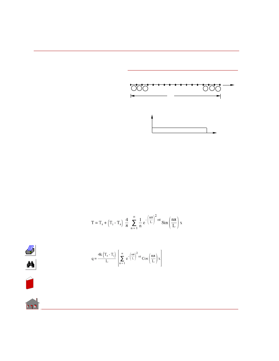
MODELING HINTS:
Since the other
dimensions of the
plate are infinitely
large, conduction
occurs through thick-
ness, i.e., along
x-axis. Therefore,
this problem can
be modeled with
one dimensional
elements having a
total length of
(L = 0.628 m) and
considering a cross
sectional area of
(A = 1 m
2
). Sixteen
TRUSS2D elements will be used to model this problem as shown in TL08-2.
ANALYTICAL SOLUTION
Let:
T
= Temperature at any point x
T
s
= Surface temperature
T
i
= Initial temperature
t
= Time
Temperature is:
(n = 1, 3, 5, ----)
Instantaneous heat flow rate per unit area at any point is:
(n = 1, 3, 5, ----)
Figure TL08-2
L
1
2
3
4
17
16
15
14
1
2
3
14 15 16
X
Finite Element Model
Temp._Time Curve
0.0
5.0
1.0
Time
Temperature
In
de
x
In
de
x
COSMOSM Advanced Modules
6-21
Part 1 HSTAR Heat Transfer Analysis
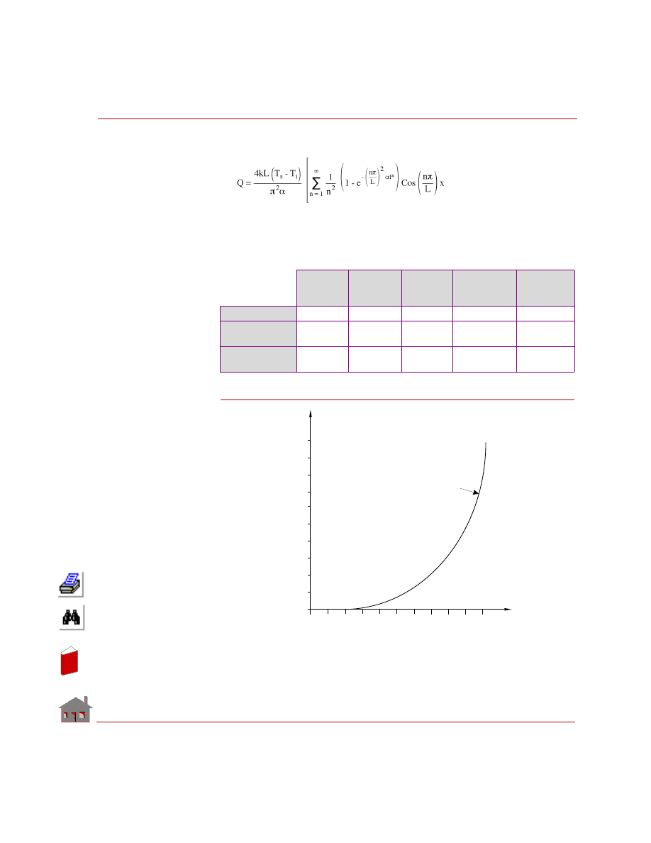
Total heat flow during time t = 0 to t* is:
(n = 1, 3, 5, ----)
COMPARISON OF RESULTS:
At time t* = 5 hours:
Figure TL08-3
Location
Distance
(m)
Location
Node No.
Theory
COSMOSM
Difference
%
Temp (T)
0.157
5
183.9
183.81
0.05
Heat Flow/
Unit Time (q)
0
1
130,880
130,030
0.65
Cumulative
Heat Flow (Q)
0
1
1,125,330
1,092,200
2.94
78.6001
2.5250
0.0500
T ime
64.3000
50.000
5.0000
Temperature Versus
Time for Node 9
T
e
m
p
e
r
a
t
u
r
e
In
de
x
In
de
x
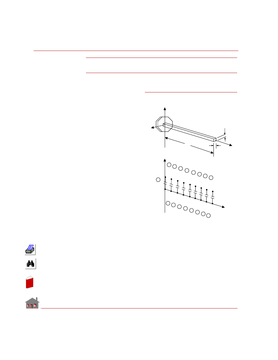
Chapter 6 Verification Problems
6-22
COSMOSM Advanced Modules
TL09: Heat Transfer from
Cooling Fin
TYPE:
Heat transfer analysis, truss
elements and convection link
elements.
REFERENCE:
Kreith, F., “Principles of Heat
Transfer,” International
Textbook Co., Scranton,
Pennsylvania, 2nd Printing,
1959.
PROBLEM:
A cooling fin of square cross-
sectional area A, length l, and
conductivity k extends from a
wall maintained at temperature
T
w
. The surface convection
coefficient between the fin and
the surrounding air is h, the air
temperature is T
a
, and the tip of
the fin is insulated. Determine
the heat conducted by the fin q
and the temperature of the tip
T
l
.
GIVEN:
b
= 1 in = (1/12) ft
Length of fin
= l = 0.667 ft
Wall temperature
= T
w
= 100
° F
Ambient temperature
= T
a
= 0
° F
Film coefficient
= h = 1 BTU/hr-ft
2
°F
Thermal conductivity
= k = 25 BTU/hr-ft
°F
Area of cross-section of the fin = 0.0069 ft
2
Figure TL09-1
Y
X
Z
1
3
5
Y
h, T
b
T
b
l
w
a
Z
1
11
12
13
18
17
16
15
9
8
7
6
5
4
3
2
14
19
7
9
11
13
15
17
16
14
12
10
8
6
4
2
In
de
x
In
de
x
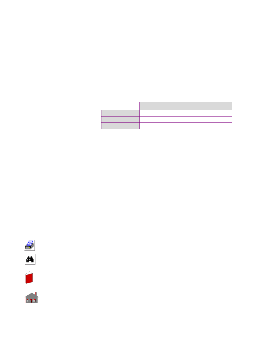
COSMOSM Advanced Modules
6-23
Part 1 HSTAR Heat Transfer Analysis
CALCULATED INPUT:
The surface convection area per inch of fin length = 0.02778 ft
2
.
MODELING HINTS:
The end convection elements are given half the surface area of the interior
convection elements. Nodes 11 through 19 are given arbitrary locations.
COMPARISON OF RESULTS:
T at Node 9,
°
F
q at Node 1, Btu/hr
Theory
68.594
17.504
COSMOSM
68.615
17.529
Difference
0.03%
0.13%
In
de
x
In
de
x
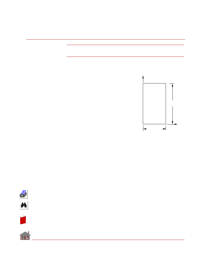
Chapter 6 Verification Problems
6-24
COSMOSM Advanced Modules
TL10: Temperature Distribution Due
to Electrical Heating in a Wire
TYPE:
Steady state heat conduction with prescribed
voltage and convection boundary conditions.
REFERENCE:
Rohsenow and Choi, “Heat, Mass and
Momentum Transfer.”
PROBLEM:
Determine the temperature distribution in a
current carrying wire. The voltage drop per
foot of the wire is 0.1 volts.
GIVEN:
Voltage on edge AB
= 0 volts
Voltage on edge DC
= -0.1 volts
Ambient temperature
= 70
° F
Thermal conductivity
= 13 Btu/hr-ft
°F
Electrical conductivity = 1.113117 E+7 mho/ft*
Heat transfer coefficient on edge BC = 5 Btu/hr-ft
2
°F
COMPARISON OF RESULTS:
Temperature at node 1 = 419.99
° F (COSMOSM)
= 420
° F (Theory)
✍
The value of the electrical conductivity coefficient already contains the con-
version factor from watt to Btu/hr.
Figure TL10-1
1.0 ft
0.03125 ft
y
x
Problem Sketch
A
B
C
D
In
de
x
In
de
x

COSMOSM Advanced Modules
6-25
Part 1 HSTAR Heat Transfer Analysis
TL11: Temperature Distribution of Air Flowing
Through a Pipe With a Constant Wall Temperature
TYPE:
Steady state fluid flow through a pipe using FLUIDT elements. The pipe is modeled
with various types of elements as follows:
TL11A 32 SHELL4 Elements
TL11B 64 SHELL3 Elements
TL11C 32 Solid Elements
TL11D 189 TETRA10 Elements
TL11E 189 TETRA4 Elements
TL11F 400 TETRA4 Elements (finer mesh)
REFERENCE:
Rhosenow and Choi, “Heat, Mass, and Momentum Transfer”.
PROBLEM:
Find the temperature distribution of air flowing through a pipe whose wall is
maintained at a constant temperature (same as problem TN06).
Figure TL11-1 Mesh of a Quarter of a Pipe with Constant Wall
Temperature and Air Flow (FLUIDT Elements)
Node at inlet is
FLUIDT Elements
outside the pipe
(prescribed
temperature)
In
de
x
In
de
x

Chapter 6 Verification Problems
6-26
COSMOSM Advanced Modules
MODELING HINTS:
•
Due to symmetry, only a quarter of the pipe circumference is modeled.
Therefore, the pipe cross sectional area and the mass flow rate to be input for
this analysis are 1/4 of the given values.
•
Air flow in the pipe is modeled by 8 FLUIDT elements. The
FLINKDEF
command is used to associate the FLUIDT elements with the pipe wall for
convection.
•
The FLUIDT elements are generated by meshing a curve along the axis of the
pipe. The curve is created such that its starting point falls outside the pipe
(below the pipe inlet). As a result, the node associated with the starting point
will not be considered for convection, and thus it can be assigned the inlet
temperature.
GIVEN:
Temperature of the pipe wall = 93.33
o
C
Temperature of air at Inlet
= 37.80
o
C
Pipe diameter
= 0.0254 m
Pipe length
= 0.127 m
Mass flow rate
= 0.000594 Kg/s
Density of Air
= 0.9611 Kg/m
3
Specific heat of air
= 1005. J/ Kg
o
K
Thermal conductivity of air
= 0.0294 W/m
o
K
Dynamic viscosity of air
= 1.566E-5 Pa-s
Parameters for evaluating
Nusselt’s number:
C1 = 1.63
C2 = 0.08
C3 = 0.7
C4 = 0.35
In
de
x
In
de
x
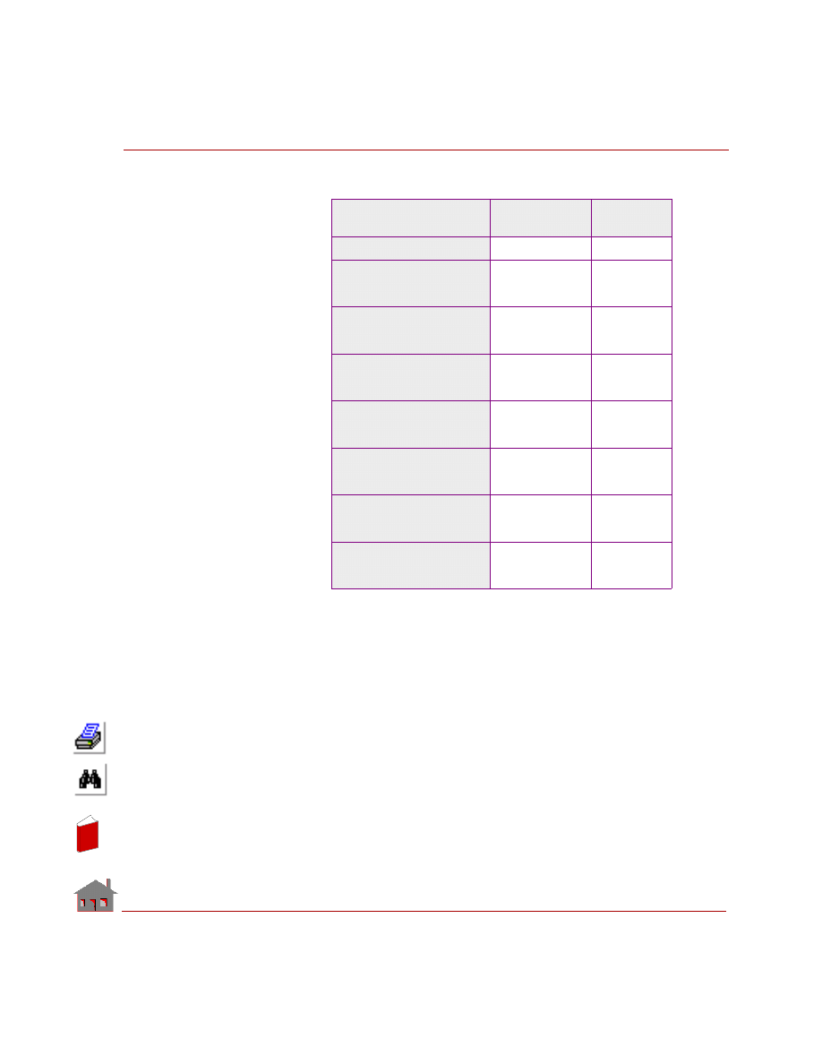
COSMOSM Advanced Modules
6-27
Part 1 HSTAR Heat Transfer Analysis
COMPARISON OF RESULTS:
Method/Element Type
Temperature of Air
at Pipe Outlet
Error
Percentage
Theory
50.5
o
C
N/A
COSMOSM
(2D HLINK Elements
(problem TN06)
49.23
o
C
- 2.51%
TL11A
(3D FLUIDT Elements
and 32 SHELL4 Elements)
51.145
o
C
1.3%
TL11B
(3D FLUIDT Elements
and 64 SHELL3 Elements)
51.145
o
C
1.3%
TL11C
(3D FLUIDT Elements
and 32 Solid Elements)
51.143
o
C
1.3%
TL11D
(3D FLUIDT Elements and
189 TETRA10 Elements)
51.243
o
C
1.5%
TL11E
(3D FLUIDT Elements and
189 TETRA4 Elements)
50.938
o
C
0.9%
TL11F
(3D FLUIDT Elements and
400 TETRA4 Elements)
51.084
o
C
1.1%
In
de
x
In
de
x
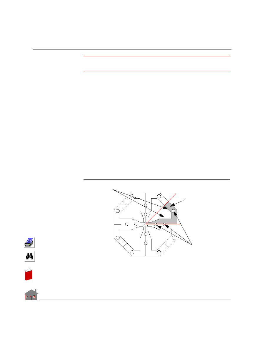
Chapter 6 Verification Problems
6-28
COSMOSM Advanced Modules
TL12: Temperature Distribution in a Linear
Accelerator with 3 Coolant Passages
TYPE:
Steady state linear heat conduction, heat convection, and fluid flow (SOLID +
FLUIDT elements)
REFERENCE:
Los Alamos National Laboratory, LANSCE Division.
PROBLEM:
Find the temperature distribution in a “Radio Frequency Quadrupole” (RFQ) with
an octagonal cross section and 3 coolant passages, due to heat flux applied to the
surfaces of the accelerator cavity. The total applied heat flux is 0.982 Btu per second
for a length of 3 inches. Water, initially at room temperature, is used as the coolant
flowing at a bulk velocity of 15 feet per second. The accelerator is made of copper.
MODELING HINTS:
The cross section of the model is shown in the figure. Due to symmetry, only 1/8 of
the model is considered.
Figure TL12-1. Cross Section of the Model
Shaded area
is 1/8 of the
model
Cooling Pipes
Heat Flux
In
de
x
In
de
x
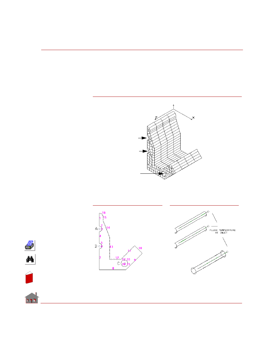
COSMOSM Advanced Modules
6-29
Part 1 HSTAR Heat Transfer Analysis
To facilitate the application of the heat flux, a thin layer of SHELL4 elements was
created (since some faces of the extruded solid elements may not be associated with
the surfaces of the polyhedron). The
FLINKDEF
command is designed to ignore
repeated areas for convection. Other data are taken from a recently completed
accelerator and are therefore realistic.
Figure TL12-2. Finite Element Model of 1/8 of a Linear
Accelerator with 3 Coolant Passages
Pipe A
Pipe B
Pipe C
Figure TL12-3.
Coolants Passages
and Corresponding
Convection Surfaces
Figure TL12-2.
Cross-section with
Coolant Passages
A, B, and C
Heat Flux applied
to surfaces 11-16
In
de
x
In
de
x

Chapter 6 Verification Problems
6-30
COSMOSM Advanced Modules
GIVEN:
Applied Heat Flux
Surface
Heat Flux Density
Heat Flux on Surface
Surfaces 11 and 12
0.0734 Btu/s/in
2
0.50646 Btu/s
Surface 13
0.0612 Btu/s/in
2
0.30924
Btu/s
Surface 14
0.0367 Btu/s/in
0.14753 Btu/s
Surface 15
0.0183 Btu/s/in
2
0.01646 Btu/s
Surface 16
0.0061 Btu/s/in
2
0.00862 Btu/s
Total Flux
0.9821 Btu/s
Properties of Solid (Copper)
Density
= 0.84E-3 lbf.s
2
/in
4
Thermal Conductivity
= 0.52E-2 Btu/in/s/
o
F
Specific Heat
= 36.0 Btu.in/lbf/s
2
/
o
F
Properties of Fluid (Water)
Density
= 0.93E-4 lbf.s
2
/in
4
(or lb/in
3
)
Thermal Conductivity
= 0.82E-5 Btu/in/s/
o
F
Specific Heat
= 390.0 Btu.in/lbf/s
2
/F (or BTU/lb/
o
F)
Viscosity
= 0.13E-6 lbf.s/in
2
(or lb/s/in)
Temperature at inlet
= 0.0
o
F (with respect to reference)
Section and Flow Properties for Passages A & B
Diameter
= 0.40 in
Flow Area
= 0.063 in
2
Bulk Velocity
= 180.0 in/s
Mass Flow rate
= .0010546 lbf.s/in (or lb/s
= (Velocity)(Density)(Area)
Film Coefficient
= .0056 Btu/in
2
/s/
o
F
Section and Flow Properties for Passage C
Diameter
= 0.50 in
Flow Area
= 0.196 in
2
Bulk Velocity
= 180.0 in/s
Mass Flow rate
= .003281 lbf.s/in (or lb/s)
In
de
x
In
de
x
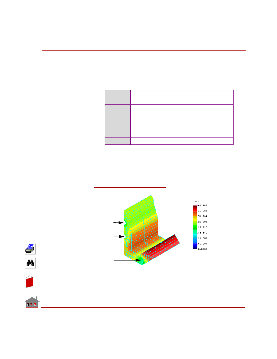
COSMOSM Advanced Modules
6-31
Part 1 HSTAR Heat Transfer Analysis
Film Coefficient
= .0056 Btu/in
2
/s/
o
F
COMPARISON OF RESULTS:
An energy balance between the applied energy (0.982 Btu/s) and the total energy
gained by the coolant (water) gives a check on results:
Where:
T
a
is the temperature at the outlet of pipe A, T
b
is the temperature at the outlet of
pipe B, and T
c
is the temperature at the outlet of pipe C. M
a
, M
b
, and M
c
are the
mass flow rates for pipes A, B, and C.
Theory
dE = (M
a
. dT
a
+ M
b
. dT
b
+ M
c
. dT
c
) (g)
= 0.982 Btu/s
COSMOSM
T
a
= 0.51323
o
F
T
b
= 0.57880
o
F
T
c
= 0.41628
o
F
dE = [(.51323) (.0010564) + (.57880) (.0010546)
+ (.41628) (.003281)] (386.) = 0.973 Btu/s
Error
= 0.916%
Figure TL12-4.
Temperature Plot
Pipe B
Pipe C
Pipe A
In
de
x
In
de
x

6-32
COSMOSM Advanced Modules
In
de
x
In
de
x

COSMOSM Advanced Modules
6-33
Part 1 HSTAR Heat Transfer Analysis
Nonlinear Heat
Transfer Analysis
In
de
x
In
de
x
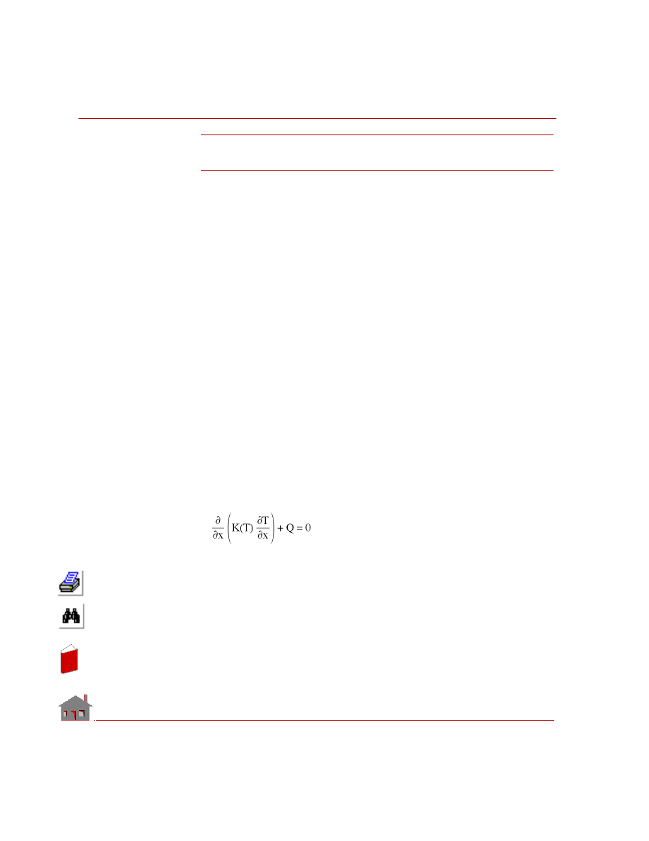
Chapter 6 Verification Problems
6-34
COSMOSM Advanced Modules
TN01: Heat Conduction with Temperature
Dependent Conductivity
TYPE:
Nonlinear heat conduction, TRUSS2D elements are used.
REFERENCE:
Ozisik, M., “Heat Conduction,” John Wiley & Sons Inc., 1980, pp. 440-443.
PROBLEM:
Determine the temperature distribution in a slab which is insulated on one face, and
subjected to a constant temperature on the other face. Assume constant internal heat
generation in the slab and a linear variation of thermal conductivity.
GIVEN:
Thickness of the slab
= L = 2 m
Internal heat generation = Q = 100,000 W/m
3
Thermal conductivity
= K = 50 (1 + 2T) W/m
°C
Boundary conditions:
At x = 0, Insulated boundary
At x = L, Prescribed temperature of 100
° C
Twenty TRUSS2D elements have been used to model this problem as shown in the
figure.
ANALYTICAL SOLUTION:
Steady state heat conduction equation is given by:
Where:
K =
K
0
(1+
β T), K
0
and
β are constants.
Q = Rate of internal heat generation.
In
de
x
In
de
x
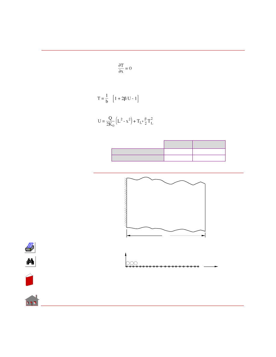
COSMOSM Advanced Modules
6-35
Part 1 HSTAR Heat Transfer Analysis
Associated boundary conditions are:
At x = 0,
At x = L, T = T
L
(Prescribed temperature)
Solution of this problem can be obtained by Kirchoff transformation as:
Where:
COMPARISON OF RESULTS:
Figure TN01-1
Theory
COSMOSM
At X = 0 (Node 1)
°
C
118.24
118.25
At X = 1 (Node 11)
°
C
113.96
113.97
Finite Element Model
Q = 100000.0 W/m
K = 50.0(1+2T) W/m C
T = 100.0 C
o
Insulated
20
L
Problem Sketch
1 2 3 4
20
1 2 3
21
Y
X
o
3
In
de
x
In
de
x
Chapter 6 Verification Problems
6-36
COSMOSM Advanced Modules
TN02: Transient Heat Conduction
(Nonlinear Analysis)
TYPE:
Nonlinear analysis, PLANE2D elements.
REFERENCES:
Aguirre-Ramirez, G., and Oden, J. T., “Finite Element Technique Applied to Heat
Conduction in Solids with Temperature Dependent Thermal Conductivity,” ASME
No. 69-WA/HT-34, November, 1969.
“Report on Finite Element Analysis of Nonlinear Heat Transfer Problems,” U. C.
Berkeley.
PROBLEM:
Determine the temperature response of an infinitely large slab of finite thickness.
The thermal conductivity assumed to vary linearly with temperature. The specific
heat is constant. Initial temperature is 100
° F and the temperature of left side
suddenly raised to 200
° F and returns to 100° F after 10 seconds.
GIVEN:
Thickness of slab
= h = 20 in
Specific heat
= c = 8 Btu-in/lb-s
2
°F
Thermal conductivity
= K(T) = 2 + 0.01 x T Btu/in-s
°F
Density of the material =
ρ = 0.25 lb-s
2
/in
4
Assumed strip length
= L = 1 in
COMPARISON OF RESULTS:
Temperature Values (F):
x
y
Node No.
3 (sec)
11 (sec)
Reference
7
0
15
103.74
125.41
COSMOSM
7
0
15
103.75
125.41
In
de
x
In
de
x
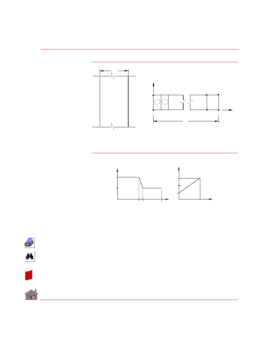
COSMOSM Advanced Modules
6-37
Part 1 HSTAR Heat Transfer Analysis
Figure TN02-1
Figure TN02-2
2
6
4
40
42
41
39
1
5
3
Finite Element Model
1
2
h
x
y
Problem Sketch
Slab
h
T
R
T = 100 F
L
0
Temp. - Time Curve
Temperature
( F)
0
100
200
0
10
20
10.000001
0
Therm. Conductivity - Temp. Curve
K
6
400
0
0
Temp.
( F)
4
2
0
In
de
x
In
de
x
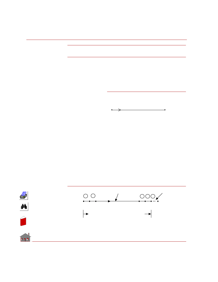
Chapter 6 Verification Problems
6-38
COSMOSM Advanced Modules
TN03: Radiation from a Rod
TYPE:
Nonlinear steady state analysis, TRUSS 2D elements and radiation link elements.
BOUNDARY CONDITIONS:
Prescribed temperatures at x = 0.
Radiation at x = 10 m.
PROBLEM:
Determine the
temperature distribution
in a rod in which the left
end has a prescribed
temperature and the right
end is radiating heat into
the ambient atmosphere.
GIVEN:
Figure TN03-2
Length of the rod
= 10 m
Area of cross section = 1 m
2
Thermal conductivity = K = 45 W/m
°C
Ambient temperature = T
∞
= 10
°C
Prescribed temp. at
left end
= T
0
= 1000
°C
Radiation Data
Area of radiating surface = 1 m
2
View factor
= 1
Emissivity
= 1
Stefan-Boltzmann
constant
= 5.67E-8
W/m
2
°K
4
Figure TN03-1
T=1000 C
T =10.0 C
Radiation
8
x
∞
∞
TRUSS 2D
RLINK
10
11
12
9
1
2
3
1
2
9
10
11
x=0
x=10
x
In
de
x
In
de
x
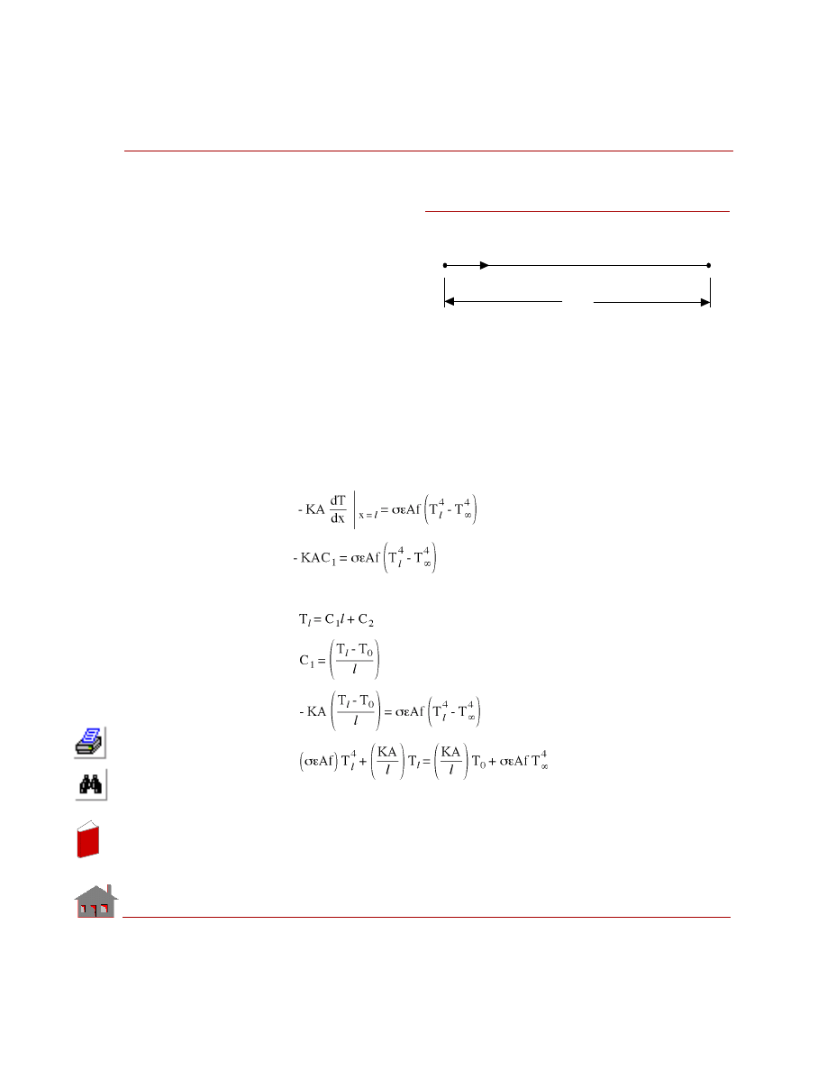
COSMOSM Advanced Modules
6-39
Part 1 HSTAR Heat Transfer Analysis
ANALYTICAL SOLUTION:
Temperature distribution
in a rod:
Boundary Conditions:
Temperature at
x = 0 T = T
0
Radiation at
x = l
Governing differential equation is:
d
2
T/dx
2
= 0
dT/dx
= C
1
T
= C
1
x + C
2
Boundary Conditions at x = 0, T = T
0
,
⇒ C
2
= T
0
at x = l
But we have
Figure TN03-3
x
T
T
l
8
0
In
de
x
In
de
x
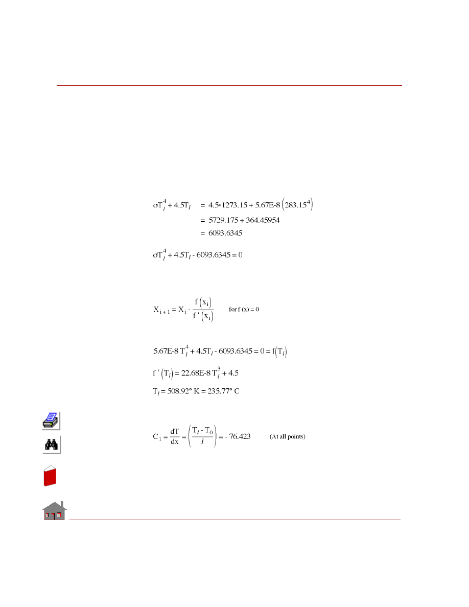
Chapter 6 Verification Problems
6-40
COSMOSM Advanced Modules
Substitute:
σ = 5.67E-8 W/m
2
°K
4
ε
= 1
f
= 1
A = 1 m
2
K = 45 W/m
°K
T
0
= 1000
° C = 1273.15 °K
T
∞
= 10
° C = 283.15 °K
Solution of the nonlinear algebraic equation, using the Newton-
Raphson method:
Let the internal heat generation Q = 0
Gradients:
In
de
x
In
de
x
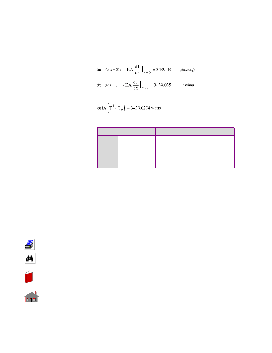
COSMOSM Advanced Modules
6-41
Part 1 HSTAR Heat Transfer Analysis
Heat flow:
This should also be equal to:
COMPARISON OF RESULTS:
Var.
x
y
z
Node
Analytical
COSMOSM
Temp
10
--
--
11
235.770
235.77
Gx
10
--
--
11
- 76.423
- 76.423
Flow
0
--
--
1
3439.030
3439.10
Flow
11
--
--
12
- 3439.020
- 3439.10
In
de
x
In
de
x
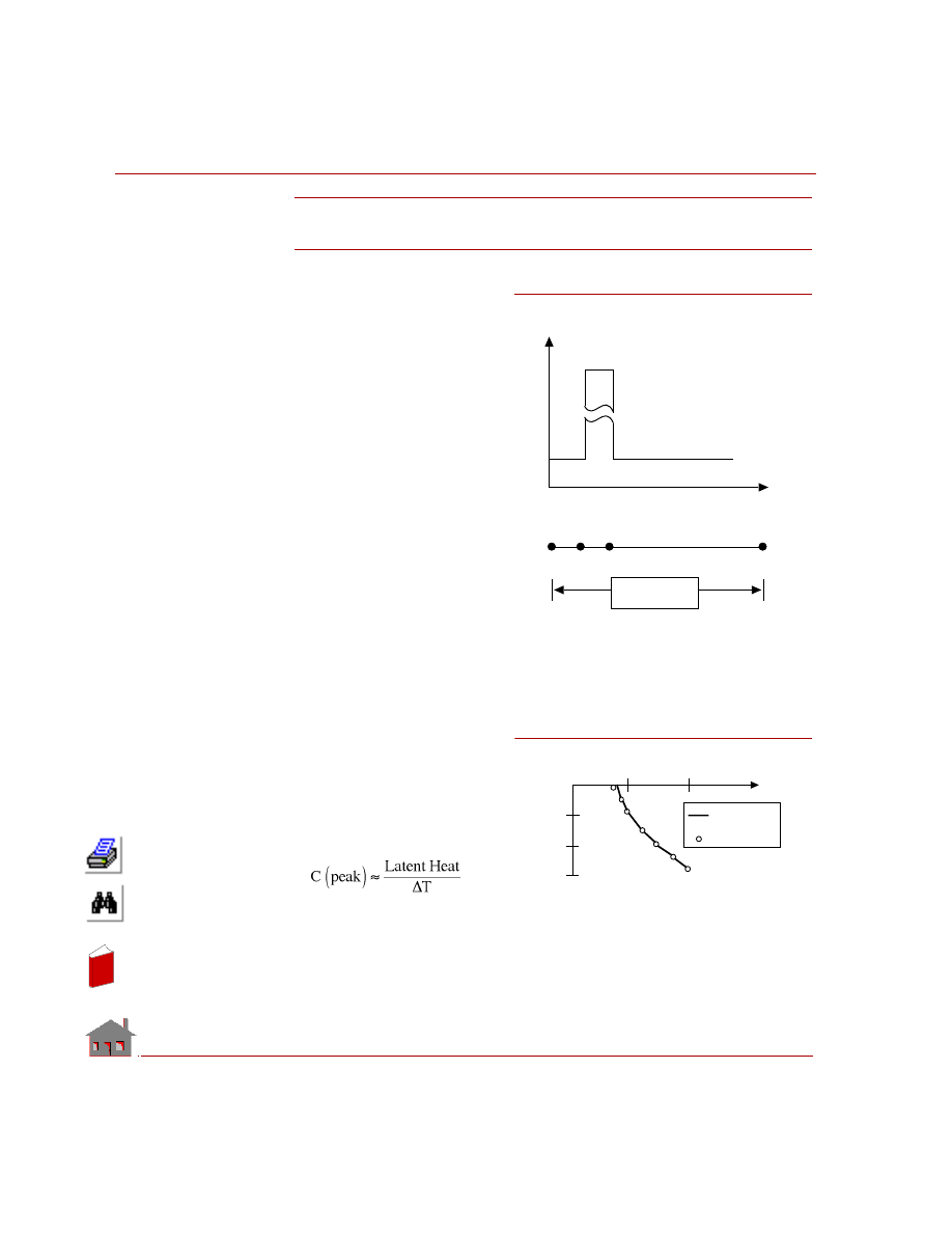
Chapter 6 Verification Problems
6-42
COSMOSM Advanced Modules
TN04: Temperature Analysis
with Phase Change
TYPE:
Thermal analysis, TRUSS 2D.
REFERENCE:
K. Morgan, R. W. Lewis, and
O. C. Zienkiewicz, “An Improved
Algorithm for Heat Conduction
Problems with Phase Change,”
International Journal of
Numerical Methods In
Engineering, Volume 12., pp.
1191 - 1195, 1978.
PROBLEM:
A uniform infinite slab of liquid
is considered to be initially at zero
degree temperature. Suddenly, the
temperature of the surface x = 0 is
reduced to -455
° F and maintained
constant. The temperature distribution in slab is calculated. The lumped heat
capacity matrix is employed and the optimal step is used in calculation.
GIVEN:
KX =
1.08
Btu/in-s
°F
DENS
= 1 lb-s
2
/in
4
C
= 1 Btu-in/lb-s
2
°F
Latent heat= 70.26 Btu/lb
MODELING HINTS:
Figure TN04-1. Finite Element Model
Temp
C
1
-1.1
-.15
70.26
1
41
2
3
4 inches
Time
-5
-10
-15
1
2
Analytical
Solution
COSMOS/M
T
e
m
per
at
ur
e
Figure TN04-2.Temperature Variation at Node 11
In
de
x
In
de
x
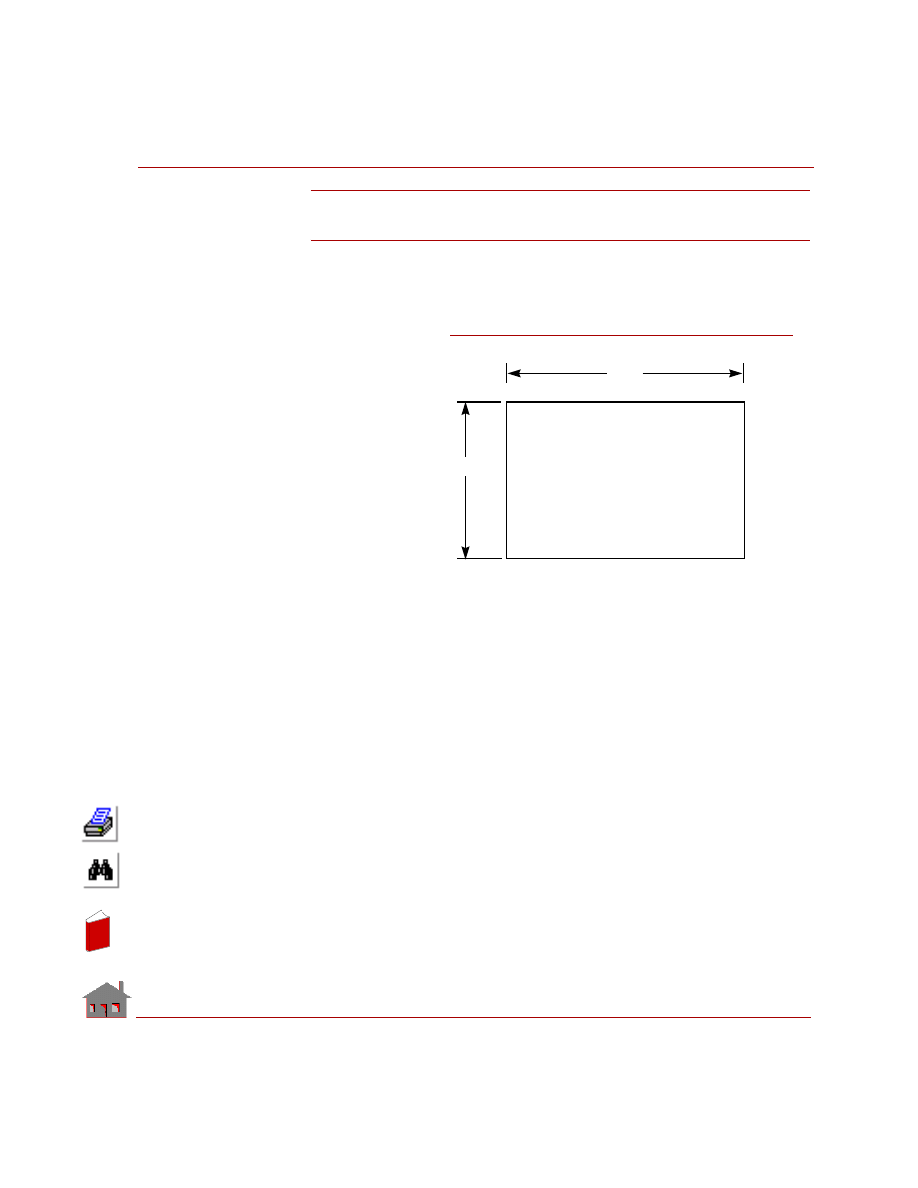
COSMOSM Advanced Modules
6-43
Part 1 HSTAR Heat Transfer Analysis
TN05: Temperature Distribution in a Slab
Exchanging Radiation with Ambient Atmosphere
TYPE:
Steady state nonlinear heat conduction problem.
REFERENCE:
R. Siegel and J. R.
Howell, “Thermal
Radiation Heat
Transfer.”
PROBLEM:
Using the radiation
enclosure theory, find
the temperature
distribution in a slab
which has a
prescribed radiation
boundary condition.
GIVEN:
COMPARISON OF RESULTS:
Temperature at node 122
= 101.7
° C (Enclosure theory)
= 101.69
° C (Radiation boundary condition)
Length of the slab
= 2.0 m
Width of the slab
= 1.0 m
Heat flux on face AD
= 10.4 w/m
2
Thermal conductivity
= 1.0 w/m-
°K
Emissivity of face BC = 0.5
Ambient temperature
= 100
° C
Stefan-Boltzmann constant
= 5.67E-8 w/m
2
-
°K
4
Convection coefficient on face AB
= 1.2 w/m
2
-
°K
T
2 m
= 0.5
D
C
Heat
Flux =
10.4
w/m
= 100
°
C
2
A
B
ε
8
1 m
T
2
h = 1.2 w/m -
°
K
= 100
°
C
8
Figure TN05-1
In
de
x
In
de
x
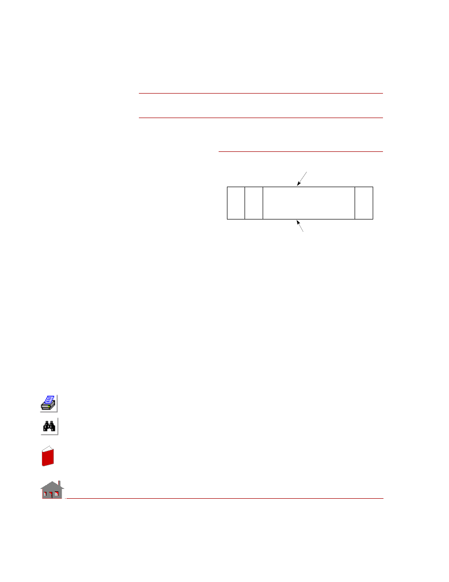
6-44
COSMOSM Advanced Modules
TN06: Temperature Distribution of Air Flowing
Through a Pipe with a Constant Wall Temperature
TYPE:
Steady state fluid flow
through a pipe.
REFERENCE:
Rhosenow and Choi,
“Heat, Mass and
Momentum Transfer.”
PROBLEM:
Find the temperature
distribution for flow of air
through a pipe whose
wall is maintained at
constant temperature.
GIVEN:
Diameter of the pipe
= 0.0254 m
Length of the pipe
= 0.127 m
Friction factor
= 0.001
Mass flow rate
= 0.000594 Kg/s
Density of air
= 0.9611Kg/m
3
Specific heat of air
= 1005 J / Kg-
°K
Thermal conductivity of air = 0.0294 w/m-
°K
Dynamic viscosity of fluid = 15.66 E-6 Pa-s
Temperature of the pipe wall = 93.33
° C
Temperature of fluid at inlet = 37.8
° C
COMPARISON OF RESULTS:
Temperature of air at pipe outlet (node 9)
= 49.23
° C (COSMOSM)
= 50.5
° C (Reference)
10
11
12
17
18
1
2
3
8
9
Pipe Wall
Pipe Axis
Figure TN06-1
In
de
x
In
de
x
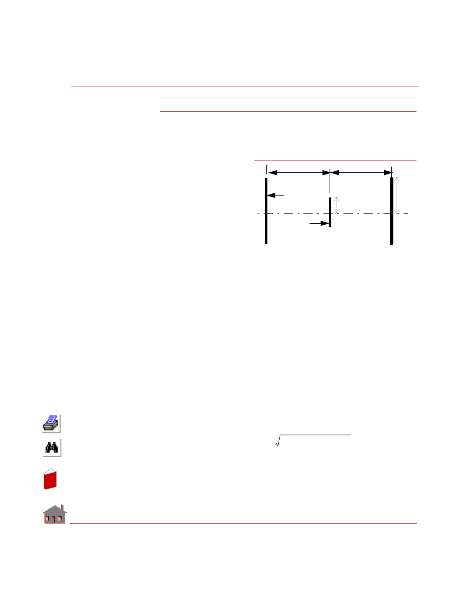
COSMOSM Advanced Modules
6-45
Part 1 HSTAR Heat Transfer Analysis
TN07: Open-System Steady State Radiation
TYPE:
Nonlinear steady state analysis, radiation in an open system.
REFERENCE:
J. P. Holman, “Heat Trans-
fer,” McGraw-Hill Book
Company, 1963, p. 193.
PROBLEM:
A 0.5-ft-diameter black disk
is placed halfway between
two black 10-ft-diameter
disks that are 20 ft apart as
shown in the figure. If the
temperature of the
surroundings is 0
o
R,
determine the steady-state
temperature of the middle disk (T
m
) if the temperature of the two outer disks is 2180
o
R.
GIVEN:
a = radius of the middle disk =0.125 ft
b = radius of each outer disk = 5 ft
l = distance between the middle disk and the outer disks = 10 ft
Stefan-Boltzmann constant =
σ = 1.714e-9 Btu/hr.ft
2
. R
4
T
env
(Temperature of the surroundings)=0
o
R
T
o
(Temperature of the outer disks)= 2180
o
R
ANALYTICAL SOLUTION:
The radiation view factor (RVF) between the outer and middle disks (F
o-m
) is
calculated from the formula:
Thus,
F
m-o
= radiation view factor from the middle disk to the outer disks = 0.19992
07
Figure TN07 Radiation of a disk
Radius of small disk = a =0.25 ft
Radius of outer disks = b = 5 ft
Distance between the middle disk
and each outer disk = l = 10 ft
l
l
Outer disk
Middle disk
b
a
F
m
o
–
l
2
a
2
b
2
l
2
a
2
b
2
+
+
(
)
2
4a
2
b
2
–
–
+
+
2a
2
(
)
⁄
=
In
de
x
In
de
x
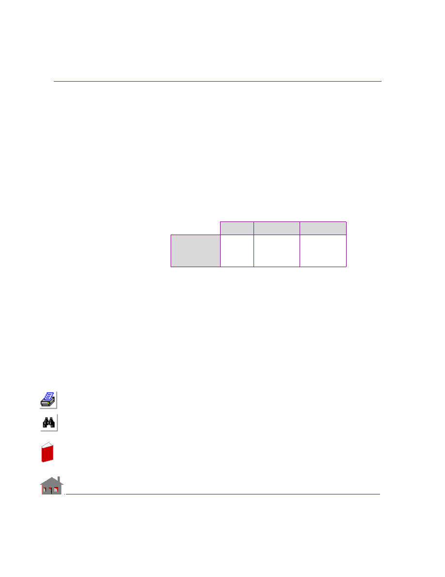
Chapter 6 Verification Problems
6-46
COSMOSM Advanced Modules
F
env
= radiation view factor from the middle disk to the environement = 1.0 -
0.19992 = 0.80008.
In steady state condition, the heat balance equation for the middle disk is given by:
Where:
σ = Stefan-Boltzmann constant
A
m
= Area of the middle disk (
πa
2
)
MODELING HINTS
Shell3 elements are used in this problem.
COMPARISON OF RESULTS:
Theory
COSMOSM
Error
Steady state
temperature of
the middle disk
(R)
1457.70
1455.68
-0.14 %
σA
m
F
env
T
m
4
T
env
4
–
(
) σ
– A
m
F
m
o
–
T
o
4
T
m
4
–
(
)
0
=
In
de
x
In
de
x
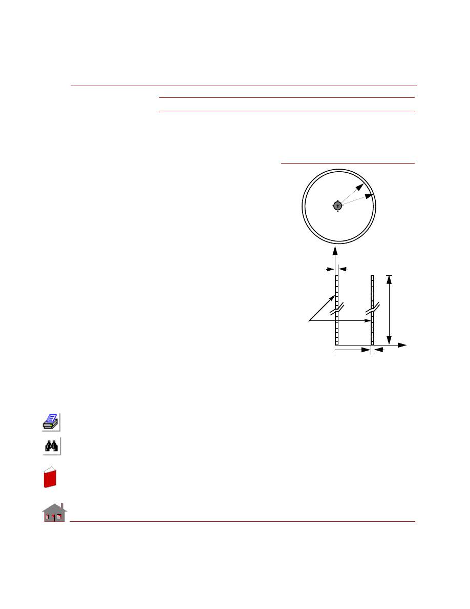
COSMOSM Advanced Modules
6-47
Part 1 HSTAR Heat Transfer Analysis
TN08: Closed-System Steady State Radiation
TYPE:
Nonlinear steady state analysis, axisymmetric radiation closed system.
REFERENCE:
J. P. Holman, “Heat Transfer,”
McGraw-Hill Book Company, 1963,
p. 191.
PROBLEM:
The temperatures of the inner and
outer concentric long cylinders shown
in the figure are maintained at 1460
o
R
and 560
o
R, respectively. Calculate the
heat transfer by radiation from inner to
the outer cylinder.
GIVEN:
Radius of the inner cylinder (r
1
)=0.1
ft
Radius of the outer cylinder (r
2
)=1.0
ft
Common length of the cylinders (l)=
100 ft
Temperature of the inner cylinder (T
1
)
=1460
o
R
Temperature of the outer cylinder (T
2
)
=560
o
R
Emissivity of the face of the inner cylinder (
ε
1
)=0.2
Emissivity of the face of the outer cylinder (
ε
2
)=0.7
Stefan-Boltzmann constant (
σ)=1.714e-9 Btu/hr.ft
2
.R
4
Figure TN08-1Two Concentric Cylinders
T
1
T
2
solid cylinder of
radius 0.1 ft
Hollow cylinder of
radii 1.0 and 1.1 ft
1.1 ft
1.0 ft
l=100 ft
Finite Element Model
0.1 ft
X
Y
1.0 ft
0.1 ft
PLANE2D
Axisymmetric
Elements
In
de
x
In
de
x
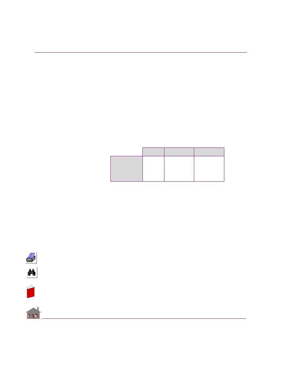
Chapter 6 Verification Problems
6-48
COSMOSM Advanced Modules
ANALYTIC SOLUTION:
The rate of heat transfer by radiation between the two cylinders is given by:
The radiation view factor between the two cylinders is F
1-2
=1.0
MODELING HINTS:
Axisymmetric PLANE2D elements are used to model this problem.
COMPARISON OF RESULTS:
Theory
COSMOSM
Error
Rate of heat
transfer
between the two
cylinders (Btu/
hr-rad)
15073.97
15076.35
0.015 %
q
1
2
–
lr
1
σ T
1
4
T
2
4
–
(
)
1
ε
1
----
1
ε
2
–
ε
2
-------------
r
1
r
2
----
+
-----------------------------------------
=
In
de
x
In
de
x
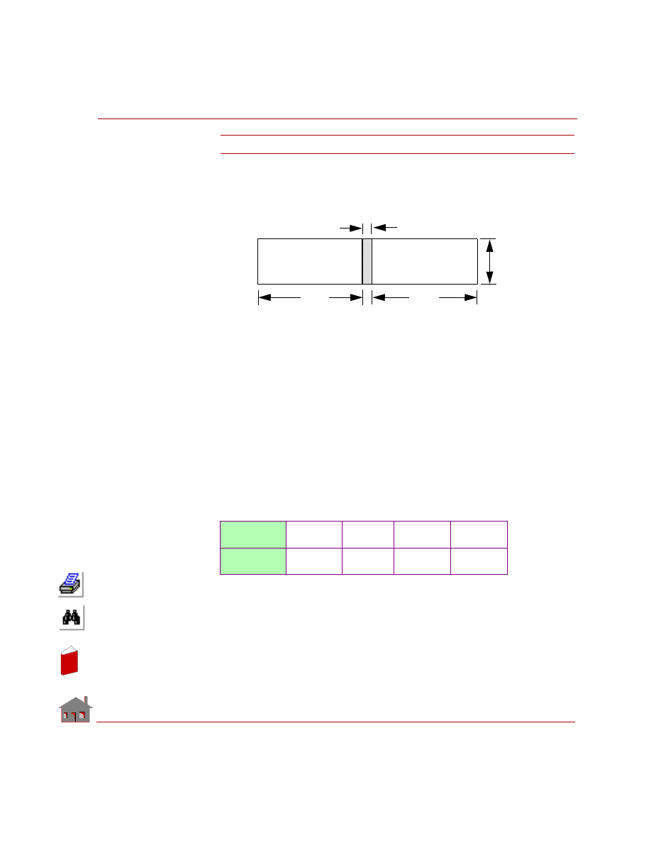
COSMOSM Advanced Modules
6-49
Part 1 HSTAR Heat Transfer Analysis
TN09A-D: Thermal Contact Through A Gap
TYPE:
Nonlinear transient analysis, SHELL4 elements.
REFERENCE:
J. P. Holman, “Heat Transfer,” McGraw-Hill Book Company, 1963, p. 191.
PROBLEM:
Block-1 and Block-2 are bonded together by a thin layer of epoxy as shown in the
figure. Both blocks are initially at 100
0
C. A temperature of 500
0
C is applied to edge
EF. Edge GH is heated to 850
0
C and then cooled back to 100
0
C. It is desired to
compute the temperature of edge AB and and the amount of heat flow between the
two blocks when edge GH is at 850
0
C, 600
0
C, and 100
0
C.
✍
The thin layer between the two blocks is modeled using GAP elements and the
conductivity of its material. This functionality avoids difficulties that otherwise
will be encountered in building the geometry and meshing complex models.
GIVEN:
Width of block-1
=0.4 m
Width of block-2
=0.5 m
Height of the block
=0.1 m
Depth of the blocks
=0.1 m
Problem Name
TN09A.GEO
TN09B.GEO
TN09C.GEO
TN09D.GEO
Element Type
SHELL4
TETRA4
SOLID
TETRA10
0.5m
0.4m
0.0035m
0.01m
A
B
C
D
E
F
G
H
Block-1
Block-2
In
de
x
In
de
x
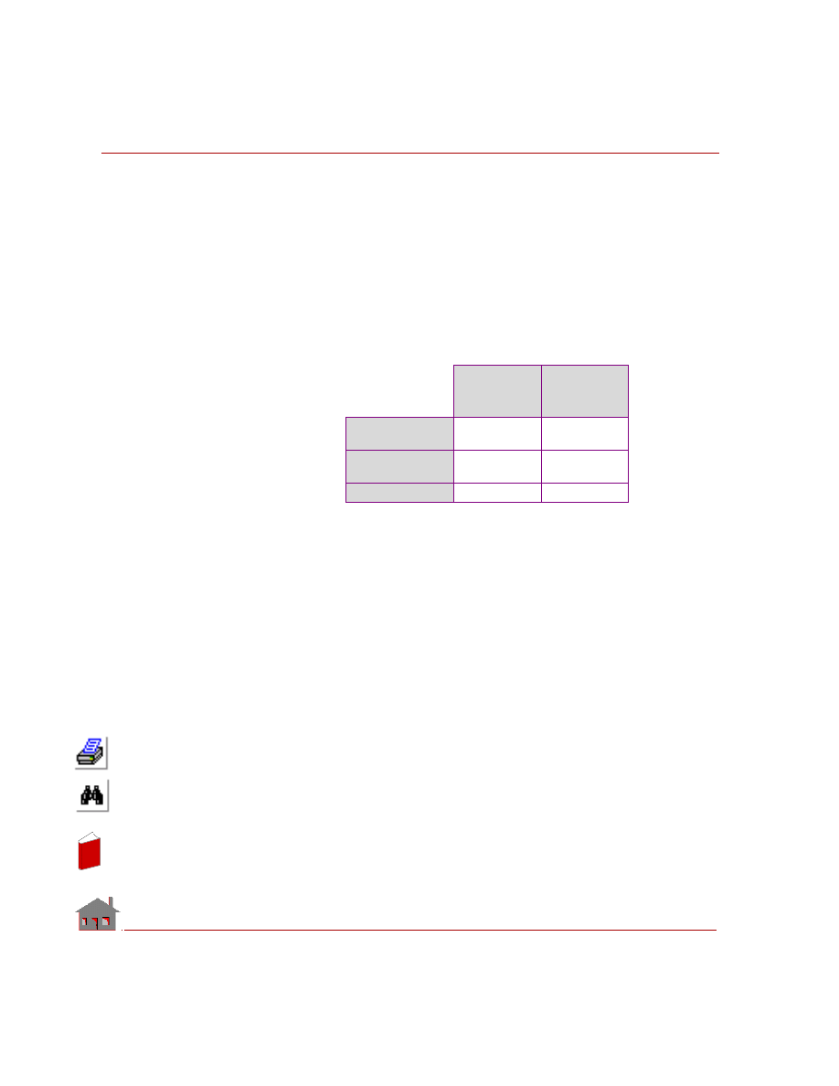
Chapter 6 Verification Problems
6-50
COSMOSM Advanced Modules
Conductivity of the blocks = KX = 250 W/m
0
C
Conductivity of the thin layer = KC= 1000 W/m
0
C
MODELING HINTS:
2D and 3D models using various types of elements are used. Automatic generation
of GAP elements is used (line-to-line for 2D models and face-to-face for 3D
models).
COMPARISON OF RESULTS:
Theory
(Temperature/
Heat Flow)
COSMOSM
(Temperature/
Heat Flow)
Edge GH at 850
0
C
636.6
0
C
8536.6 W
636.6
0
C
8536.6 W
Edge GH at 600
0
C
539.0
0
C
2439.0W
636.6
0
C
8536.6 W
Edge GH at 100
0
C
????
???
In
de
x
In
de
x

COSMOSM Advanced Modules
6-51
Part 1 HSTAR Heat Transfer Analysis
In
de
x
In
de
x

Chapter 6 Verification Problems
6-52
COSMOSM Advanced Modules
In
de
x
In
de
x

COSMOSM Advanced Modules
I-1
Index
A
ambient atmosphere
axisymmetric
B
bond sets
bonding
boundary conditions
C
coefficient of permeability
6-14
conduction
constant heat generation
convection
convection coefficient
convection link
convective heat transfer
D
density
E
electric current flow
electrical conductivity
electromagnetic waves
4-5
elements for HSTAR
equation
F
film coefficients
fluid flow
G
governing equation
H
heat capacity matrix
heat conduction
heat flux
heat generation
6-34
heat generation rate
heat transfer analysis
heat transfer coefficient
I
initial temperature
J
Joule heating
L
latent heat
M
N
nodal heat generation
nodal temperature
nonlinear analysis
nonlinear heat conduction
nonlinear steady state
analysis
P
phase change
In
de
x
In
de
x

Index
I-2
COSMOSM Advanced Modules
piezometric head
potential flow
primary bond entity
R
radiation
radiation exchange
radiation link
real constants
recharge
S
seepage flow problem
specific heat
static analysis
steady state
steady state heat conduction
Stefan-Boltzmann constant
stream function formulation
streamlines
T
target entities
temperature dependent
temperature gradient
thermal analysis
thermal bonding
thermal conductivity
4-1, 5-2, 5-3, 5-5, 6-5, 6-18, 6-34,
thermal stress analysis
thermal stresses
thermostat
THSTAT
time curve
time curves
transfer coefficient
transient
transient heat conduction
transient problem
V
velocity potential
formulations
view factors
voltage
voltage drop
In
de
x
In
de
x
Document Outline
- COSMOSM Thermal Analysis Module (HSTAR)
- 1 Introduction
- 2 Analysis
- Introduction
- Steady State Analysis
- Transient Analysis
- Radiation View Factor Calculation
- Thermo-Electric Coupling
- Loads and Boundary Conditions
- Time and Temperature Curves
- Thermal Stress Analysis
- Bonding of Meshes with Noncompatible Elements
- Guidelines for Using the Bond Capability
- Phase Change
- Thermostat
- 3 Description of Elements
- 4 Brief Description of Commands
- 5 Detailed Examples
- 6 Verification Problems
- Index
Wyszukiwarka
Podobne podstrony:
Module ThermalAnalysis 1
Microwaves in organic synthesis Thermal and non thermal microwave
Module 10
Module 8
Food ćwiczenia angielski Starland 1 module 8
Instrukcja montażu sufitów podwieszanych w module 600x600mm System standardowy 600x600 1 AMF REINRAU
AT Commands for Bluetooth Module
Module 07
CISCO CCNA Certifications CCNA 2 Module 10
CISCO CCNA Certifications CCNA 2 Module 9
Module 12
CISCO CCNA Certifications CCNA 2 Module 1
delta module1 sample test01 1
06 BS Module 1 Section 6
CISCO CCNA Certifications CCNA 3 Module 3
53 755 765 Effect of Microstructural Homogenity on Mechanical and Thermal Fatique
Module 11
więcej podobnych podstron