
Practical Artificial Intelligence Programming in Java
Version 1.2, last updated January 1, 2006.
by Mark Watson.
This work is licensed under the Creative Commons Attribution NoDerivs NonCommercial License.
Additional license terms:
No commercial use without author's permission
The work is published "AS IS" with no implied or expressed warranty - you accept all risks for the use of both the
Free Web Book and any software program examples that are bundled with the work.
This web book may be distributed freely in an unmodified form. Please report any errors to
markw@markwatson.com
and look occasionally at Open Content (Free Web Books) at
www.markwatson.com
for
newer versions.
Requests from the author
I live in a remote area, the mountains of Northern Arizona and work remotely via the Internet. Although I really enjoy
writing Open Content documents like this Web Book and working on Open Source projects, I earn my living as a
consultant. I specialize in artificial intelligence applications, software design, and development in Java, Common Lisp,
and Ruby. Please keep me in mind for consulting jobs!

Table of Contents
Table of Contents........................................................................................................................................................................................2
Preface........................................................................................................................................................................................................5
Acknowledgements........................................................................................................................................................................................... ......5
Introduction................................................................................................................................................................................................6
Notes for users of UNIX and Linux..................................................................................................................................................................... ..7
Use of the Unified Modeling Language (UML) in this book........................................................................................................ .......................7
Chapter 1. Search.....................................................................................................................................................................................10
1.1 Representation of State Space, Nodes in Search Trees and Search Operators................................................................................10
1.2 Finding paths in mazes................................................................................................................................................................................ ...12
1.3 Finding Paths in Graphs.................................................................................................................................................................. ..............19
1.4 Adding heuristics to Breadth First Search................................................................................................................................................... .26
1.5 Search and Game Playing................................................................................................................................................................... ...........27
1.5.1 Alpha-Beta search................................................................................................................................................................................................................27
1.5.2 A Java Framework for Search and Game Playing................................................................................................................................................................28
1.5.3 TicTacToe using the alpha beta search algorithm................................................................................................................................................................33
1.5.4 Chess using the alpha beta search algorithm........................................................................................................................................................................38
Chapter 2. Natural Language Processing...............................................................................................................................................46
2.1 ATN Parsers........................................................................................................................................................................................ ............47
2.1.1 Lexicon data for defining word types..................................................................................................................................................................................50
2.1.2 Design and implementation of an ATN parser in Java.........................................................................................................................................................51
2.1.3 Testing the Java ATN parser.................................................................................................................................................................................................57
2.2 Using Prolog for NLP........................................................................................................................................................................ .............58
2.2.1 Prolog examples of parsing simple English sentences.........................................................................................................................................................58
2.2.2 Embedding Prolog rules in a Java application.....................................................................................................................................................................61
Chapter 3. Expert Systems........................................................................................................................................................................64
3.1 A tutorial on writing expert systems with Jess....................................................................................................................... ......................64
3.2 Implementing a reasoning system with Jess................................................................................................................................. ................70
3.3 Embedding Jess Expert Systems in Java Programs.................................................................................................................................... .74

Chapter 4. Genetic Algorithms.................................................................................................................................................................78
4.1 Java classes for Genetic Algorithms.................................................................................................................................................... ..........81
4.2 Example System for solving polynomial regression problems..................................................................................................................... 85
Chapter 5. Neural networks.....................................................................................................................................................................89
5.1 Hopfield neural networks............................................................................................................................................................................... 90
5.2 Java classes for Hopfield neural networks.................................................................................................................................................... 91
5.3 Testing the Hopfield neural network example class.......................................................................................................................... ...........93
5.5 Backpropagation neural networks................................................................................................................................................. ...............95
5.6 A Java class library and examples for using back propagation neural networks........................................................................ ..............97
5.7 Solving the XOR Problem...................................................................................................................................................................... ......105
5.8 Notes on using back propagation neural networks.................................................................................................................... ................106
6. Machine Learning using Weka..........................................................................................................................................................108
6.1 Using machine learning to induce a set of production rules.............................................................................................................. ........108
6.2 A sample learning problem....................................................................................................................................................... ...................109
6.3 Running Weka............................................................................................................................................................................................... 110
Chapter 7. Statistical Natural Language Processing............................................................................................................................112
7.1 Hidden Markov Models................................................................................................................................................................................ 112
7.2 Training Hidden Markov Models.................................................................................................................................................. ..............114
7.3 Using the trained Markov model to tag text................................................................................................................................ ...............116
Chapter 8. Bayesian Networks...............................................................................................................................................................117
Bibliography............................................................................................................................................................................................118
Index........................................................................................................................................................................................................120

For my grandson Calvin and granddaughter Emily

1
Preface
This book was written for both professional programmers and home hobbyists who already know how to program in Java and who
want to learn practical AI programming techniques. I have tried to make this a fun book to work through. In the style of a “cook
book”, the chapters in this book can be studied in any order. Each chapter follows the same pattern: a motivation for learning a
technique, some theory for the technique, and a Java example program that you can experiment with.
Acknowledgements
I would like to thank Kevin Knight for writing a flexible framework for game search algorithms in Common LISP (Rich, Knight
1991) and for giving me permission to reuse his framework, rewritten in Java; the game search Java classes in Chapter 1 were loosely
patterned after this Common LISP framework and allows new games to be written by sub classing three abstract Java classes. I would
like to thank Sieuwert van Otterloo for writing the Prolog in Java program and for giving me permission to use it in this free web
book. I would like to thank Ernest J. Friedman-Hill at Sandia National Laboratory for writing the Jess expert system toolkit. I would
like to thank Christopher Manning and Hinrich Schutze for writing their “Foundations of Statistical Natural Language Processing”
book; it is one of the most useful textbooks that I own. I would like to thank my wife Carol for her support in both writing this book,
and all of my other projects. I would also like to acknowledge the use of the following fine software tools: IntelliJ Java IDE and the
Poseidon UML modeling tool (
www.gentleware.com
).

2
Introduction
This book provides the theory of many useful techniques for AI programming. There are relatively few source code listings in this
book, but complete example programs that are discussed in the text should have been included in the same ZIP file that contained this
web book. If someone gave you this web book without the examples, you can download an up to date version of the book and
examples on the Open Content page of
www.markwatson.com
.
All the example code is covered by the Gnu Public License (GPL). If the GPL prevents you from using any of the examples in this
book, please contact me for other licensing terms.
The code examples all consist of either reusable (non GUI) libraries and throw away test programs to solve a specific application
problem; in some cases, the application specific test code will contain a GUI written in JFC (Swing). The examples in this book
should be included in the same ZIP file that contains the PDF file for this free web book. The examples are found in the subdirectory
src that contains:
src
src/expertsystem - Jess rule files
src/expertsystem/weka - Weka machine learning files
src/ga - genetic algorithm code
src/neural - Hopfield and Back Propagation neural network code
src/nlp
src/nlp/Markov - a part of speech tagger using a Markov model
src/nlp/prolog - NLP using embedded Prolog
src/prolog - source code for Prolog engine written by Sieuwert van Otterloo
src/search
src/search/game - contains alpha-beta search framework and tic-tac-toe and chess examples
src/search/statespace
src/search/statespace/graphexample - graph search code
src/search/statespace/mazeexample - maze search code
To run any example program mentioned in the text, simply change directory to the src directory that was created from the example
program ZIP file from my web site. Individual example programs are in separate subdirectories contained in the src directory. Typing
"javac *.java" will compile the example program contained in any subdirectory, and typing "java Prog" where Prog is the file name of
the example program file with the file extension ".java" removed. None of the example programs (except for the NLBean natural
language database interface) is placed in a separate package so compiling the examples will create compiled Java class files in the
current directory.

3
I have been interested in AI since reading Bertram Raphael's excellent book "Thinking Computer: Mind Inside Matter" in the early
1980s. I have also had the good fortune to work on many interesting AI projects including the development of commercial expert
system tools for the Xerox LISP machines and the Apple Macintosh, development of commercial neural network tools, application of
natural language and expert systems technology, application of AI technologies to Nintendo and PC video games, and the application
of AI technologies to the financial markets. I enjoy AI programming, and hopefully this enthusiasm will also infect the reader.
Notes for users of UNIX and Linux
I use Mac OS X, Linux and Windows 2000 for my Java development. To avoid wasting space in this book, I show examples for
running Java programs and sample batch files for Windows only. If I show in the text an example of running a Java program that uses
JAR files like this:
java -classpath nlbean.jar;idb.jar NLBean
the conversion to UNIX or Linux is trivial; replace “;” with “:” like this:
java -classpath nlbean.jar:idb.jar NLBean
If I show a command file like this c.bat file:
javac -classpath idb.jar;. -d . nlbean/*.java
jar cvf nlbean.jar nlbean/*.class
del nlbean\*.class
Then a UNIX/Linux (or Mac OS X) equivalent using bash might look like this:
#!/bin/bash
javac -classpath idb.jar:. -d . nlbean/*.java
jar cvf nlbean.jar nlbean/*.class
rm -f nlbean/*.class
Use of the Unified Modeling Language (UML) in this book
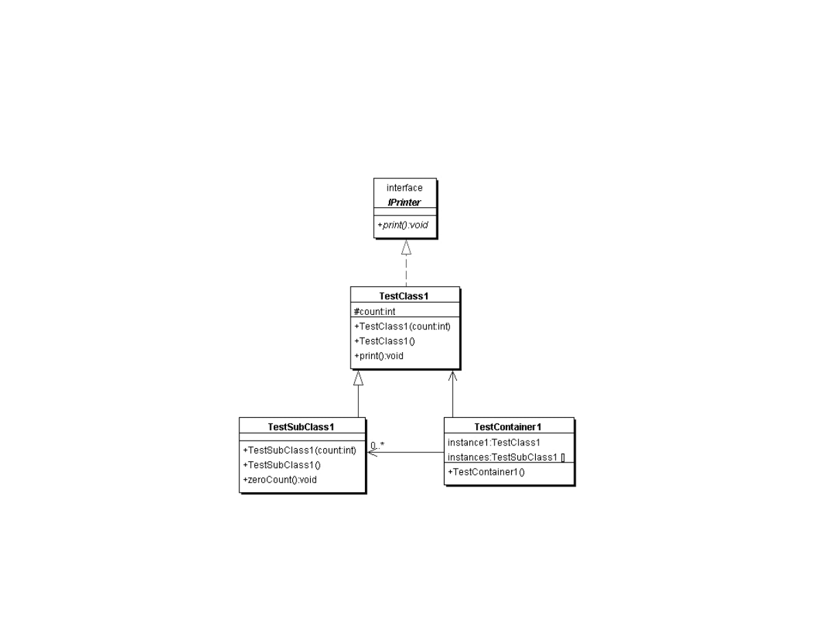
In order to discuss some of the example code in this book, I use Unified Modeling Language (UML) class diagrams. Figure 1 shows a
simple UML class diagram that introduces the UML elements used in other diagrams in this book. Figure 1 contains one Java interface

4
Iprinter and three Java classes TestClass1, TestSubClass1, and TestContainer1. The following listing shows these classes and
interface that do nothing except provide an example for introducing UML:
Listing 1 – Iprinter.java
public interface IPrinter {
public void print();
}
Listing 2 – TestClass1.java
public class TestClass1 implements IPrinter {
protected int count;
public TestClass1(int count) { this.count = count; }
public TestClass1() { this(0); }
public void print() { System.out.println("count="+count); }
}
Listing 3 – TestSubClass1.java
public class TestSubClass1 extends TestClass1 {
public TestSubClass1(int count) { super(count); }
public TestSubClass1() { super(); }
public void zeroCount() { count = 0; }
}
Listing 4 TestContainer1.java
public class TestContainer1 {
public TestContainer1() { }
TestClass1 instance1;
TestSubClass1 [] instances;
}
Again, the code in Listings 1 through 4 is just an example to introduce UML. In Figure 1, note that both the interface and classes are
represented by a shaded box; the interface I labeled. The shaded boxes have three sections:
●
Top section – name of the interface or class
●
Middle section – instance variables
●
Bottom section – class methods
In Figure 1, notice that we have three types of arrows:
5
●
Dotted line with a solid arrowhead – indicates that TestClass1 implements the interface Iprinter
●
Solid line with a solid arrowhead – indicates that TestSubClass1 is derived from the base class TestClass1
●
Solid line with lined arrowhead – used to indicate containment. The unadorned arrow from class TestContainer1 to TestClass1
indicates that the class TestContainer1 contains exactly one instance of the class TestClass1. The arrow from class
TestContainer1 to TestSubClass1 is adorned: the 0..* indicates that the class TestContainer1 can contain zero or more instances
of class TestSubClass1
Figure 1. Sample UML class diagram showing one Java interface and three Java classes
This simple UML example should be sufficient to introduce the concepts that you will need to understand the UML class diagrams in
this book.

6
Chapter 1. Search
Early AI research emphasized the optimization of search algorithms. This approach made a lot of sense because many AI tasks can be
solved by effectively by defining state spaces and using search algorithms to define and explore search trees in this state space. Search
programs were frequently made tractable by using heuristics to limit areas of search in these search trees. This use of heuristics
converts intractable problems to solvable problems by compromising the quality of solutions; this trade off of less computational
complexity for less than optimal solutions has become a standard design pattern for AI programming. We will see in this chapter that
we trade off memory for faster computation time and better results; often, by storing extra data we can make search time faster, and
make future searches in the same search space even more efficient.
What are the limitations of search? Early on, search applied to problems like checkers and chess mislead early researchers into
underestimating the extreme difficulty of writing software that performs tasks in domains that require general world knowledge or
deal with complex and changing environments. These types of problems usually require the understanding and then the
implementation of domain specific knowledge.
In this chapter, we will use three search problem domains for studying search algorithms: path finding in a maze, path finding in a
static graph, and alpha-beta search in the games: tic-tac-toe and chess. The examples in this book should be included in the examples
ZIP file for this book. The examples for this chapter are found in the subdirectory src that contains:
●
src
●
src/search
●
src/search/game – contains alpha-beta search framework and tic-tac-toe and chess examples
●
src/search/statespace
●
src/search/statespace/graphexample – graph search code
●
src/search/statespace/mazeexample – maze search code
1.1 Representation of State Space, Nodes in Search Trees and Search Operators
We will use a single search tree representation in graph search and maze search examples in this chapter. Search trees consist of nodes
that define locations in state space and links to other nodes. For some small problems, the search tree can be easily specified
statically; for example, when performing search in game mazes, we can precompute a search tree for the state space of the maze. For
many problems, it is impossible to completely enumerate a search tree for a state space so we must define successor node search
operators that for a given node produce all nodes that can reached from the current node in one step; for example, in the game of
7
chess we can not possibly enumerate the search tree for all possible games of chess, so we define a successor node search operator that
given a board position (represented by a node in the search tree) calculates all possible moves for either the white or black pieces. The
possible chess moves are calculated by a successor node search operator and are represented by newly calculated nodes that are linked
to the previous node. Note that even when it is simple to fully enumerate a search tree, as in the game maze example, we still might
want to generate the search tree dynamically as we will do in this chapter).
For calculating a search tree we use a graph. We will represent graphs as node with links between some of the nodes. For solving
puzzles and for game related search, we will represent positions in the search space with Java objects called nodes. Nodes contain
arrays of references to both child and parent nodes. A search space using this node representation can be viewed as a directed graph
or a tree. The node that has no parent nodes is the root node and all nodes that have no child nodes a called leaf nodes.
Search operators are used to move from one point in the search space to another. We deal with quantized search spaces in this chapter,
but search spaces can also be continuous in some applications. Often search spaces are either very large or are infinite. In these cases,
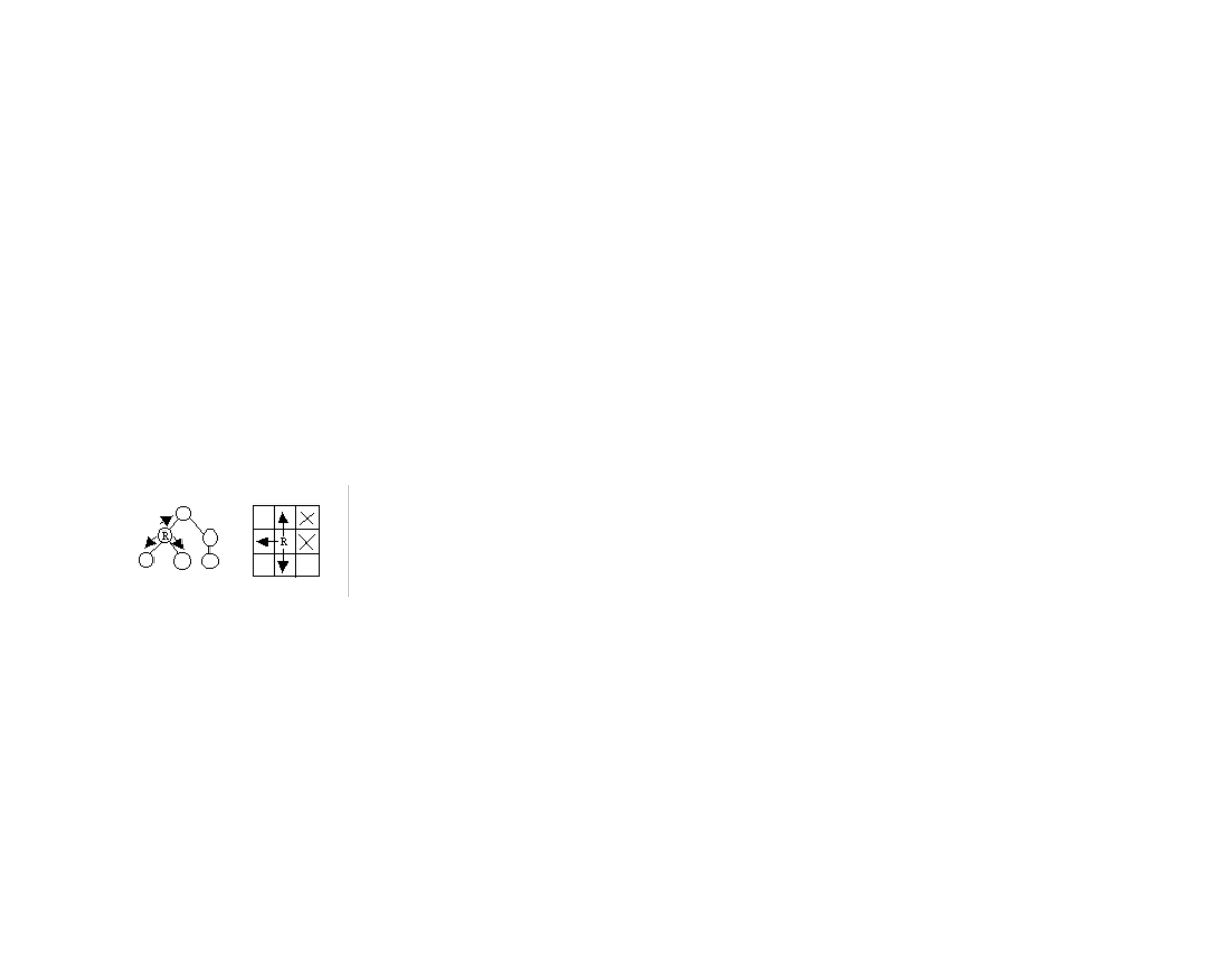
we implicitly define a search space using some algorithm for extending the space from our reference position in the space. Figure 1.1
shows representations of search space as both connected nodes in a graph and as a two-dimensional grid with arrows indicating
possible movement from a reference point denoted by R.
Figure 1.1 a directed graph (or tree) representation is shown on the left and a two-dimensional grid (or maze) representation is
shown on the right. In both representations, the letter R is used to represent the current position (or reference point) and the
arrowheads indicate legal moves generated by a search operator. In the maze representation, the two grid cells are marked
with an X indicate that a search operator cannot generate this grid location.
When we specify a search space as a two-dimensional array, search operators will move the point of reference in the search space from
a specific grid location to an adjoining grid location. For some applications, search operators are limited to moving up/down/left/right
and in other applications; operators can additionally move the reference location diagonally.
When we specify a search space using node representation, search operators can move the reference point down to any child node or
up to the parent node. For search spaces that are represented implicitly, search operators are also responsible for determining legal
child nodes, if any, from the reference point.

8
Note: I use slightly different libraries for the maze and graph search examples. I plan to clean up this code in the future and have a
single abstract library to support both maze and graph search examples.
1.2 Finding paths in mazes
The example program used in this section is MazeSearch.java in the directory src/search/maze and I assume that the reader has
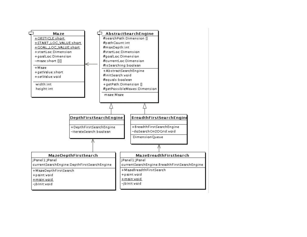
downloaded the entire example ZIP file for this book and placed the source files for the examples in a convenient place. Figure 1.2
shows the UML class diagram for the maze search classes: depth first and breadth first search. The abstract base class
AbstractSearchEngine contains common code and data that is required by both the classes DepthFirstSearch and
BreadthFirstSearch. The class Maze is used to record the data for a two-dimensional maze, including which grid locations contain
walls or obstacles. The class Maze defines three static short integer values used to indicate obstacles, the starting location, and the
ending location.
9
Figure 1.2 UML class diagram for the maze search Java classes
The Java class Maze defines the search space. This class allocates a two-dimensional array of short integers to represent the state of
any grid location in the maze. Whenever we need to store a pair of integers, we will use an instance of the standard Java class
java.awt.Dimension, which has two integer data components: width and height. Whenever we need to store an x-y grid location, we

10
create a new Dimension object (if required), and store the x coordinate in Dimension.width and the y coordinate in
Dimension.height. As in the right hand side of Figure 1.1, the operator for moving through the search space from given x-y
coordinates allows a transition to any adjacent grid location that is empty. The Maze class also contains the x-y location for the
starting location (startLoc) and goal location (goalLoc). Note that for these examples, the class Maze sets the starting location to grid
coordinates 0-0 (upper left corner of the maze in the figures to follow) and the goal node in (width – 1)-(height – 1) (lower right corner
in the following figures).
The abstract class AbstractSearchEngine is the base class for both DepthFirstSearchEngine and BreadthFirstSearchEngine. We
will start by looking at the common data and behavior defined in AbstractSearchEngine. The class constructor has two required
arguments: the width and height of the maze, measured in grid cells. The constructor defines an instance of the Maze class of the
desired size and then calls the utility method initSearch to allocate an array searchPath of Dimension objects, which will be used to
record the path traversed through the maze. The abstract base class also defines other utility methods:
●
equals(Dimension d1, Dimension d2) – checks to see if two Dimension arguments are the same
●
getPossibleMoves(Dimension location) – returns an array of Dimension objects that can be moved to from the specified
location. This implements the movement operator.
Now, we will look at the depth first search procedure. The constructor for the derived class DepthFirstSearchEngine calls the base
class constructor and then solves the search problem by calling the method iterateSearch. We will look at this method in some detail.
The arguments to iterate search specify the current location and the current search depth:
private void iterateSearch(Dimension loc, int depth) {
The class variable isSearching is used to halt search, avoiding more solutions, once one path to the goal is found.
if (isSearching == false) return;
We set the maze value to the depth for display purposes only:
maze.setValue(loc.width, loc.height, (short)depth);
Here, we use the super class getPossibleMoves method to get an array of possible neighboring squares that we could move to; we
then loop over the four possible moves (a null value in the array indicates an illegal move):
Dimension [] moves = getPossibleMoves(loc);
for (int i=0; i<4; i++) {
if (moves[i] == null) break; // out of possible moves
// from this location

11
Record the next move in the search path array and check to see if we are done:
searchPath[depth] = moves[i];
if (equals(moves[i], goalLoc)) {
System.out.println("Found the goal at " +
moves[i].width +
", " + moves[i].height);
isSearching = false;
maxDepth = depth;
return;
} else {
If the next possible move is not the goal move, we recursively call the iterateSearch method again, but starting from this new location
and increasing the depth counter by one:
iterateSearch(moves[i], depth + 1);
if (isSearching == false) return;
}
}
return;
}
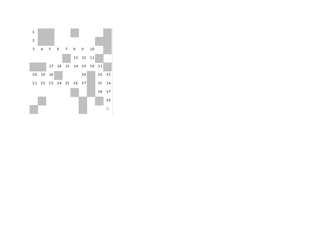
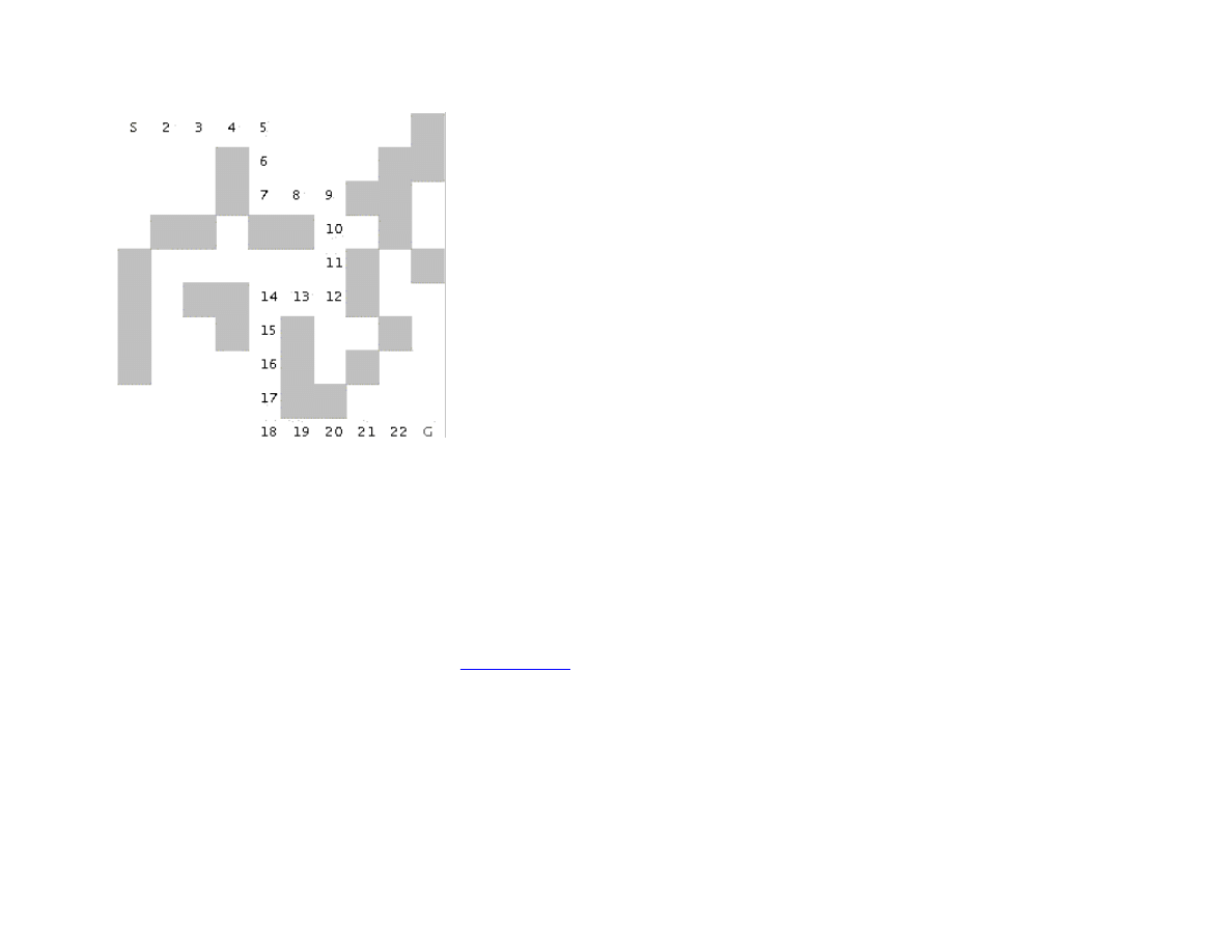
Figure 1.3 shows how poor of a path a depth first search can find between the start and goal locations in the maze. The maze is a 10 by
10 grid. The letter S marks the starting location in the upper left corner and the goal position is marked with a G in the lower right
hand corner of the grid. Blocked grid cells are painted light gray. The basic problem with the depth first search is that the search
engine will often start searching in a bad direction, but still find a path eventually, even given a poor start. The advantage of a depth
first search over a breadth first search is that the depth first search requires much less memory. We will see that possible moves for
depth first search are stored on a stack (last in, first out data structure) and possible moves for a breadth first search are stored in a
queue first in, first out data structure).
12
Figure 1.3 Using depth first search to find a path in a maze finds a non-optimal solution
The derived class BreadthFirstSearch is similar to the DepthFirstSearch procedure with one major difference: from a specified
search location, we calculate all possible moves, and make one possible trial move at a time. We use a queue data structure for storing
possible moves, placing possible moves on the back of the queue as they are calculated, and pulling test moves from the front of the
queue. The effect of a breadth first search is that it “fans out” uniformly from the starting node until the goal node is found.
The class constructor for BreadthFirstSearch calls the super class constructor to initialize the maze, and then uses the auxiliary
method doSearchOn2Dgrid for performing a breadth first search for the goal. We will look at the method BreadthFirstSearch in some
detail. The class DimensionQueue implements a standard queue data structure that handles instances of the class Dimension.
The method doSearchOn2Dgrid is not recursive, it uses a loop to add new search positions to the end of an instance of class
DimensionQueue and to remove and test new locations from the front of the queue. The two-dimensional array allReadyVisited keeps
us from searching the same location twice. To calculate the shortest path after the goal is found, we use the predecessor array:
private void doSearchOn2DGrid() {
int width = maze.getWidth();
int height = maze.getHeight();
boolean alReadyVisitedFlag[][] =
new boolean[width][height];
Dimension predecessor[][] = new Dimension[width][height];
DimensionQueue queue = new DimensionQueue();
for (int i=0; i<width; i++) {

13
for (int j=0; j<height; j++) {
alReadyVisitedFlag[i][j] = false;
predecessor[i][j] = null;
}
}
We start the search by setting the already visited flag for the starting location to true value and adding the starting location to the back
of the queue:
alReadyVisitedFlag[startLoc.width][startLoc.height]
= true;
queue.addToBackOfQueue(startLoc);
boolean success = false;
This outer loop runs until either the queue is empty of the goal is found:
outer:
while (queue.isEmpty() == false) {
We peek at the Dimension object at the front of the queue (but do not remove it) and get the adjacent locations to the current position
in the maze:
Dimension head = queue.peekAtFrontOfQueue();
Dimension [] connected = getPossibleMoves(head);
We loop over each possible move; if the possible move is valid (i.e., not null) and if we have not already visited the possible move
location, then we add the possible move to the back of the queue and set the predecessor array for the new location to the last square
visited (head is the value from the front of the queue). If we find the goal, break out of the loop:
for (int i=0; i<4; i++) {
if (connected[i] == null) break;
int w = connected[i].width;
int h = connected[i].height;
if (alReadyVisitedFlag[w][h] == false) {
alReadyVisitedFlag[w][h] = true;
predecessor[w][h] = head;
queue.addToBackOfQueue(connected[i]);
if (equals(connected[i], goalLoc)) {
success = true;
break outer; // we are done
}
}
}

14
We have processed the location at the front of the queue (in the variable head), so remove it:
queue.removeFromFrontOfQueue();
}
Now that we are out of the main loop, we need to use the predecessor array to get the shortest path. Note that we fill in the searchPath
array in reverse order, starting with the goal location:
maxDepth = 0;
if (success) {
searchPath[maxDepth++] = goalLoc;
for (int i=0; i<100; i++) {
searchPath[maxDepth] =
predecessor[searchPath[maxDepth - 1]
.width][searchPath[maxDepth - 1].height];
maxDepth++;
if (equals(searchPath[maxDepth - 1], startLoc))
break; // back to starting node
}
}
}
Figure 1.4 shows a good path solution between starting and goal nodes. Starting from the initial position, the breadth first search
engine adds all possible moves to the back of a queue data structure. For each possible move added to this queue in one search cycle,
all possible moves are added to the queue for each new move recorded. Visually, think of possible moves added to the queue, as
“fanning out” like a wave from the starting location. The breadth first search engine stops when this “wave” reaches the goal location.
In general, I prefer breadth first search techniques to depth first search techniques when memory storage for the queue used in the
search process is not an issue. In general, the memory requirements for performing depth first search is much less than breadth first
search.
15
Figure 1.4 Using breadth first search in a maze to find an optimal solution
To run the two example programs from this section, change directory to src/search/maze and type:
javac *.java
java MazeDepthFirstSearch
java MazeBreadthFirstSearch
Note that the classes MazeDepthFirstSearch and MazeBreadthFirstSearch are simple Java JFC applications that produced Figures
1.3 and 1.4. The interested reader can read through the source code for the GUI test programs, but we will only cover the core AI code
in this book. If you are interested in the GUI test programs and you are not familiar with the Java JFC (or Swing) classes, there are
several good tutorials on JFC programming at
java.sun.com
.
1.3 Finding Paths in Graphs
In the last section, we used both depth first and breadth first search techniques to find a path between a starting location and a goal
location in a maze. Another common type of search space is represented by a graph. A graph is a set of nodes and links. We
characterize nodes as containing the following data:
A name and/or other data

16
Zero or more links to other nodes
A position in space (this is optional, usually for display or visualization purposes)
Links between nodes are often called edges. The algorithms used for finding paths in graph are very similar to finding paths in a two-
dimensional maze. The primary difference is the operators that allow us to move from one node to another. In the last section, we saw
that in a maze, an agent can move from one grid space to another if the target space is empty. For graph search, a movement operator
allows movement to another node if there is a link to the target node.
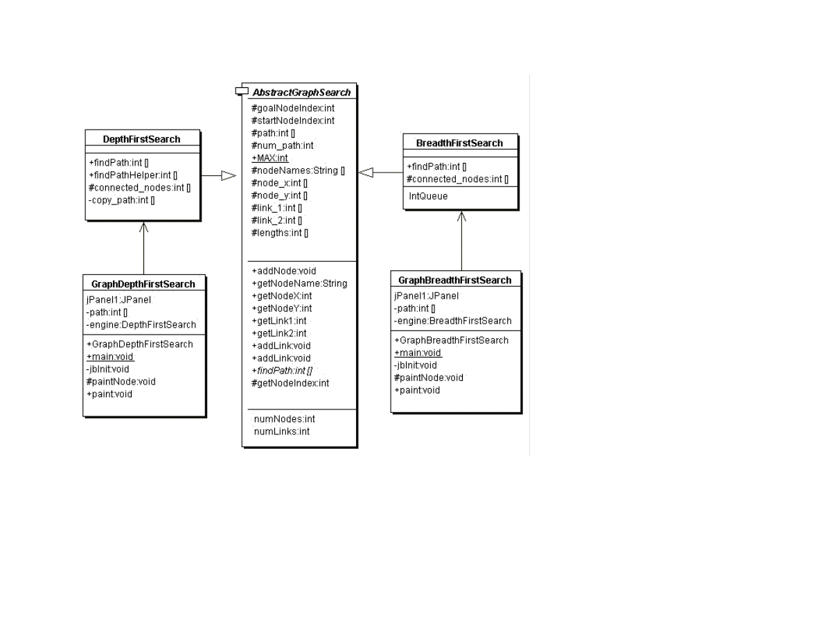
Figure 1.5 shows the UML class diagram for the graph search Java classes that we will use in this section. The abstract class
AbstractGraphSearch class is the base class for both DepthFirstSearch and BreadthFirstSearch. The classes GraphDepthFirstSearch
and GraphBreadthFirstSearch and test programs that also provide a Java Foundation Class (JFC) or Swing based user interface. These
two test programs produced Figures 1.6 and 1.7.
17
Figure 1.5 UML class diagram for the graph search classes
As seen in Figure 1.5, most of the data for the search operations (i.e., nodes, links, etc.) is defined in the abstract class
AbstractGraphSearch. This abstract class is customized through inheritance to use a stack for storing possible moves (i.e., the array
path) for depth first search and a queue for breadth first search.
The abstract class AbstractGraphSearch allocates data required by both derived classes:
final public static int MAX = 50;
protected int [] path = new int[AbstractGraphSearch.MAX];
protected int num_path = 0;

18
// for nodes:
protected String [] nodeNames = new String[MAX];
protected int [] node_x = new int[MAX];
protected int [] node_y = new int[MAX];
// for links between nodes:
protected int [] link_1 = new int[MAX];
protected int [] link_2 = new int[MAX];
protected int [] lengths = new int[MAX];
protected int numNodes = 0;
protected int numLinks = 0;
protected int goalNodeIndex = -1, startNodeIndex = -1;
The abstract base class also provides several common utility methods:
addNode(String name, int x, int y) – adds a new node
addLink(int n1, int n2) – adds a bidirectional link between nodes indexed by n1 and n2. Node indexes start at zero and are in the
order of calling addNode.
addLink(String n1, String n2) - adds a bidirectional link between nodes specified by their names
getNumNodes() – returns the number of nodes
getNumLinks() – returns the number of links
getNodeName(int index) – returns a node’s name
getNodeX(), getNodeY() – return the coordinates of a node
getNodeIndex(String name) – gets the index of a node, given its name
The abstract base class defines an abstract method that must be overridden:
public int [] findPath(int start_node, int goal_node)
We will start with the derived class DepthFirstSearch, looking at its implementation of findPath.
The findPath method returns an array of node indices indicating the calculated path:
public int [] findPath(int start_node, int goal_node) {
The class variable path is an array that is used for temporary storage; we set the first element to the starting node index, and call the
utility method findPathHelper:
path[0] = start_node; // the starting node
return findPathHelper(path, 1, goal_node);
}

19
The method findPathHelper is the interesting method in this class that actually performs the depth first search; we will look at it in
some detail:
The path array is used as a stack to keep track of which nodes are being visited during the search. The argument num_path is the
number of locations in the path, which is also the search depth:
public int [] findPathHelper(int [] path, int num_path,
int goal_node) {
First, re check to see if we have reached the goal node; if we have, make a new array of the current size and copy the path into it. This
new array is returned as the value of the method:
if (goal_node == path[num_path - 1]) {
int [] ret = new int[num_path];
for (int i=0; i<num_path; i++) ret[i] = path[i];
return ret; // we are done!
}
We have not found the goal node, so call the method connected_nodes to find all nodes connected to the current node that are not
already on the search path (see the source code for the implementation of connected_nodes):
int [] new_nodes = connected_nodes(path, num_path);
If there are still connected nodes to search, add the next possible node to visit to the top of the stack (variable path) and recursively
call findPathHelper again:
if (new_nodes != null) {
for (int j=0; j<new_nodes.length; j++) {
path[num_path] = new_nodes[j];
int [] test = findPathHelper(new_path,
num_path + 1,
goal_node);
if (test != null) {
if (test[test.length - 1] == goal_node) {
return test;
}
}
}
}
If we have not found the goal node, return null, instead of an array of node indices:

20
return null;
}
The derived class BreadthFirstSearch also must define the abstract method findPath. This method is very similar to the breadth first
search method used for finding a path in a maze: a queue is used to store possible moves. For a maze, we used a queue class that
stored instances of the class Dimension; so for this problem, the queue only needs to store integer node indices. The return value of
findPath is an array of node indices that make up the path from the starting node to the goal.
public int [] findPath(int start_node, int goal_node) {
We start by setting up a flag array alreadyVisited to prevent visiting the same node twice, and allocating a predecessors array that we
will use to find the shortest path once the goal is reached:
// data structures for depth first search:
boolean [] alreadyVisitedFlag = new boolean[numNodes];
int [] predecessor = new int[numNodes];
The class IntQueue is a private class defined in the file BreadthFirstSearch.java; it implements a standard queue:
IntQueue queue = new IntQueue(numNodes + 2);
Before the main loop, we need to initialize the already visited and predecessor arrays, set the visited flag for the starting node to true,
and add the starting node index to the back of the queue:
for (int i=0; i<numNodes; i++) {
alreadyVisitedFlag[i] = false;
predecessor[i] = -1;
}
alreadyVisitedFlag[start_node] = true;
queue.addToBackOfQueue(start_node);
The main loop runs until either we find the goal node or the search queue is empty:
outer:
while (queue.isEmpty() == false) {
We will read (without removing) the node index at the front of the queue and calculate the nodes that are connected to the current node
(but not already on the visited list) using the connected_nodes method (the interested reader can see the implementation in the source
code for this class):
int head = queue.peekAtFrontOfQueue();
int [] connected = connected_nodes(head);
if (connected != null) {

21
For each node connected by a link to the current node, if it has not already been visited set the predecessor array and add the new node
index to the back of the search queue; we stop if the goal is found:
for (int i=0; i<connected.length; i++) {
if (alreadyVisitedFlag[connected[i]] == false) {
predecessor[connected[i]] = head;
queue.addToBackOfQueue(connected[i]);
if (connected[i] == goal_node) break outer;
}
}
alreadyVisitedFlag[head] = true;
queue.removeFromQueue(); // ignore return value
}
}
Now that the goal node has been found, we can build a new array of returned node indices for the calculated path using the
predecessor array:
int [] ret = new int[numNodes + 1];
int count = 0;
ret[count++] = goal_node;
for (int i=0; i<numNodes; i++) {
ret[count] = predecessor[ret[count - 1]];
count++;
if (ret[count - 1] == start_node) break;
}
int [] ret2 = new int[count];
for (int i=0; i<count; i++) {
ret2[i] = ret[count - 1 - i];
}
return ret2;
}
In order to run both the depth first and breadth first graph search examples, change directory to JavaAI2/src/search/graph and type
the following commands:
javac *.java
java GraphDepthFirstSearch
java GraphBeadthFirstSearch
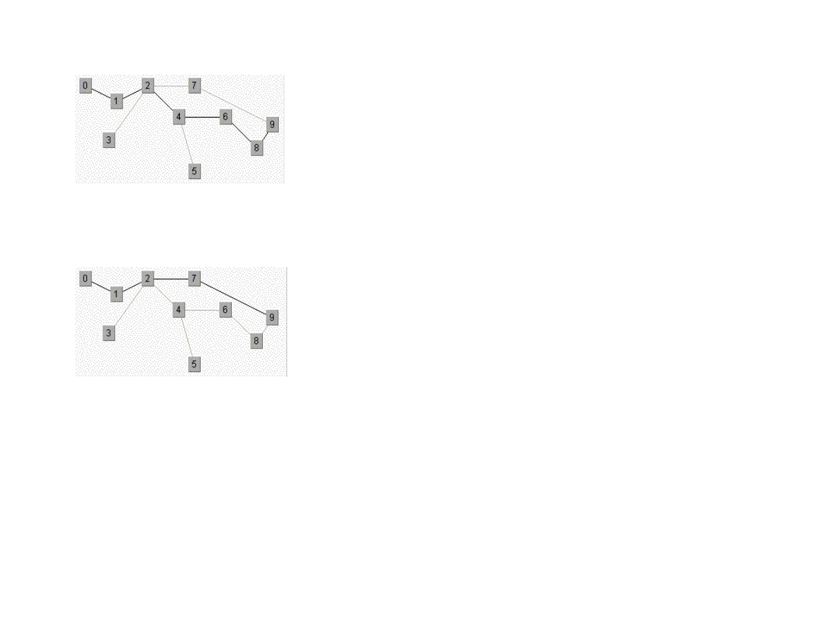
Figure 1.6 shows the results of finding a route from node 1 to node 9 in the small test graph. Like the depth first results seen in the
maze search, this path is not optimal.
22
Figure 1.6 Using depth first search in a sample graph
Figure 1.7 shows an optimal path found using a breadth first search. As we saw in the maze search example, we find optimal solutions
using breadth first search at the cost of extra memory required for the breadth first search.
Figure 1.7 Using breadth first search in a sample graph
1.4 Adding heuristics to Breadth First Search
We can usually make breadth first search more efficient by ordering the search order for all branches from a given position in the
search space. For example, when adding new nodes, from a specified reference point in the search space, we might want to add nodes
to the search queue first that are “in the direction” of the goal location: in a two-dimensional search like our maze search, we might
want to search connected grid cells first that were closest to the goal grid space. In this case, pre-sorting nodes (in order of closest
distance to the goal) added to the breadth first search queue could have a dramatic effect on search efficiency. In the next chapter, we
will build a simple real-time planning system around our breadth first maze search program; this new program will use heuristics. The
alpha beta additions to breadth first search are seen in Section 1.5.

23
1.5 Search and Game Playing
Now that a computer program has won a match against the human world champion, perhaps people’s expectations of AI systems will
be prematurely optimistic. Game search techniques are not real AI, but rather, standard programming techniques. A better platform for
doing AI research is the game of Go. There are so many possible moves in the game of Go, that brute force look ahead (as is used in
Chess playing programs) simply does not work.
That said, min-max type search algorithms with alpha-beta cutoff optimizations are an important programming technique and will be
covered in some detail in the remainder of this chapter. We will design an abstract Java class library for implementing alpha-beta
enhanced min-max search, and then use this framework to write programs to play tic-tac-toe and chess.
1.5.1 Alpha-Beta search
The first game that we will implement will be tic-tac-toe, so we will use this simple game to explain how the min-max search (with
alpha-beta cutoffs) works.
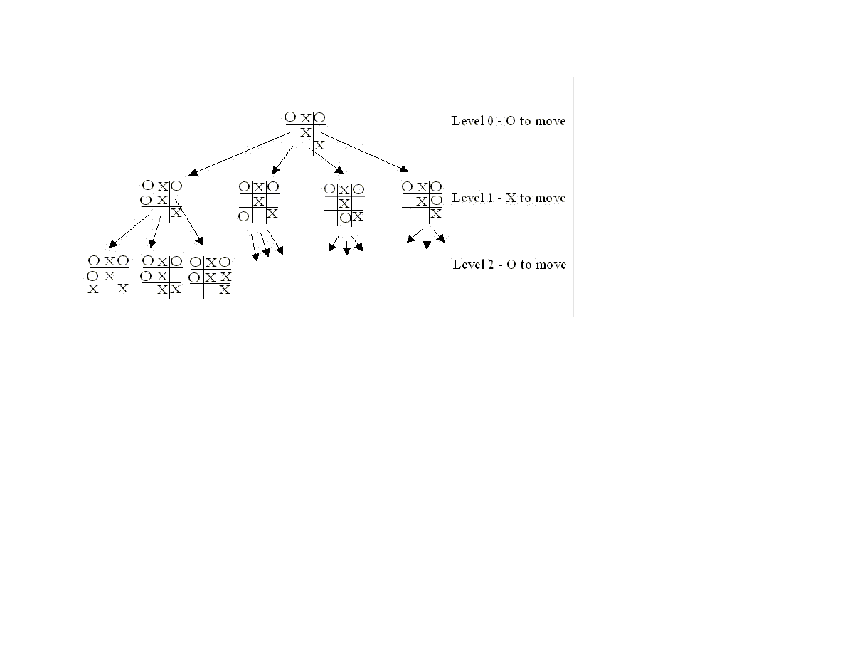
Figure 1.8 shows the possible moves generated from a tic-tac-toe position where X has made three moves and O has made 2 moves; it
is O’s turn to move. This is “level 0” in Figure 1.8. At level 0, O has four possible moves. How do we assign a fitness values to each of
O’s possible moves at level 0? The basic min-max search algorithm provides a simple solution to this problem: for each possible move
by O in level 1, make the move and store the resulting 4 board positions. Now, at level 1, it is X’s turn to move. How do we assign
values to each of X’s possible three moves in Figure 1.8? Simple, we continue to search by making each of X’s possible moves and
storing each possible board position for level 2. We keep recursively applying this algorithm until we either reach a maximum search
depth, or there is a win, loss, or draw detected in a generated move. We assume that there is a fitness function available that rates a
given board position relative to either side. Note that the value of any board position for X if the negative of the value for O.
24
Figure 1.8 Alpha-beta algorithm applied to part of a game of tic-tac-toe.
To make the search more efficient, we maintain values for alpha and beta for each search level. Alpha and beta determine the best
possible/worst possible move available at a given level. If we reach a situation, like the second position in level 2, where X has won,
then we can immediately determine that O’s last move in level 1 that produced this position (of allowing X an instant win) is a low
valued move for O (but a high valued move for X). This allows us to immediately “prune” the search tree by ignoring all other
possible positions arising from the first O move in level 1. This alpha-beta cutoff (or tree pruning) procedure can save a large
percentage of search time, especially if we can set the search order at each level with “probably best” moves considered first.
While tree diagrams as seen in Figure 1.8 quickly get complicated, it is easy for a computer program to generate possible moves,
calculate new possible board positions and temporarily store them, and recursively apply the same procedure to the next search level
(but switching min-max “sides” in the board evaluation). We will see in the next section that it only requires about 100 lines of Java
code to implement an abstract class framework for handling the details of performing an alpha-beta enhanced search. The additional
game specific classes for tic-tac-toe require about an additional 150 lines of code to implement; chess requires an additional 450 lines
of code.
1.5.2 A Java Framework for Search and Game Playing

25
The general interface for the Java classes that we will develop in this section was inspired by the Common LISP game-playing
framework written by Kevin Knight and described in (Rich, Knight 1991). The abstract class GameSearch contains the code for
running a two-player game and performing an alpha-beta search. This class needs to be sub classed to provide the eight methods:
public abstract boolean drawnPosition(Position p)
public abstract boolean wonPosition(Position p,
boolean player)
public abstract float positionEvaluation(Position p,
boolean player)
public abstract void printPosition(Position p)
public abstract Position [] possibleMoves(Position p,
boolean player)
public abstract Position makeMove(Position p, boolean player,
Move move)
public abstract boolean reachedMaxDepth(Position p,
int depth)
public abstract Move getMove()
The method drawnPosition should return a Boolean true value if the given position evaluates to a draw situation. The method
wonPosition should return a true value if the input position is won for the indicated player. By convention, I use a Boolean true value
to represent the computer and a Boolean false value to represent the human opponent. The method positionEvaluation returns a
position evaluation for a specified board position and player. Note that if we call positionEvaluation switching the player for the
same board position, then the value returned is the negative of the value calculated for the opposing player. The method
possibleMoves returns an array of objects belonging to the class Position. In an actual game, like chess, the position objects will
actually belong to a chess-specific refinement of the Position class (e.g., for the chess program developed later in this chapter, the
method possibleMoves will return an array of ChessPosition objects). The method makeMove will return a new position object for a
specified board position, side to move, and move. The method reachedMaxDepth returns a Boolean true value if the search process
has reached a satisfactory depth. For the tic-tac-toe program, the method reachedMaxDepth does not return true unless either side has
won the game or the board is full; for the chess program, the method reachedMaxDepth returns true is the search has reached a depth
of 4 have moves deep (this is not the best strategy, but it has the advantage of making the example program short and easy to
understand). The method getMove returns an object of a class derived from the class Move (e.g., TicTacToeMove or ChessMove).
The GameSearch class implements the following methods to perform game search:
protected Vector alphaBeta(int depth, Position p, boolean player)
protected Vector alphaBetaHelper(int depth, Position p,
boolean player,
float alpha, float beta)
public void playGame(Position startingPosition,
boolean humanPlayFirst)

26
The method alphaBeta is simple; it calls the helper method alphaBetaHelper with initial search conditions; the method
alphaBetaHelper then calls itself recursively. The code for alphaBeta is:
protected Vector alphaBeta(int depth, Position p,
boolean player)
{
Vector v = alphaBetaHelper(depth, p, player,
1000000.0f, -1000000.0f);
return v;
}
It is important to understand what is in the vector returned by the methods alphaBeta and alphaBetaHelper. The first element is a
floating point position evaluation for the point of view of the player whose turn it is to move; the remaining values are the “best move”
for each side to the last search depth. As an example, if I let the tic-tac-toe program play first, it placed a marker at square index 0,
then I placed my marker in the center of the board an index 4. At this point, to calculate the next computer move, alphaBeta is called
and returns the following elements in a vector:
next element: 0.0
next element: [-1,0,0,0,1,0,0,0,0,]
next element: [-1,1,0,0,1,0,0,0,0,]
next element: [-1,1,0,0,1,0,0,-1,0,]
next element: [-1,1,0,1,1,0,0,-1,0,]
next element: [-1,1,0,1,1,-1,0,-1,0,]
next element: [-1,1,1,1,1,-1,0,-1,0,]
next element: [-1,1,1,1,1,-1,-1,-1,0,]
next element: [-1,1,1,1,1,-1,-1,-1,1,]
Here, the alpha-beta enhanced min-max search looked all the way to the end of the game and these board positions represent what the
search procedure calculated as the best moves for each side. Note that the class TicTacToePosition (derived from the abstract class
Position) has a toString method to print the board values to a string.
The same printout of the returned vector from alphaBeta for the chess program is:
next element: 5.4
next element:
[4,2,3,5,9,3,2,4,7,7,1,1,1,0,1,1,1,1,7,7,0,0,0,0,0,0,0,0,7,7,0,0,0,1,0,0,0,0,7,7,0,0,0,0,0,0,0,0,7,7,0,0,0,
0,-1,0,0,0,7,7,-1,-1,-1,-1,0,-1,-1,-1,7,7,-4,-2,-3,-5,-9,-3,-2,-4,]
next element:
[4,2,3,0,9,3,2,4,7,7,1,1,1,5,1,1,1,1,7,7,0,0,0,0,0,0,0,0,7,7,0,0,0,1,0,0,0,0,7,7,0,0,0,0,0,0,0,0,7,7,0,0,0,
0,-1,0,0,0,7,7,-1,-1,-1,-1,0,-1,-1,-1,7,7,-4,-2,-3,-5,-9,-3,-2,-4,]
next element:
[4,2,3,0,9,3,2,4,7,7,1,1,1,5,1,1,1,1,7,7,0,0,0,0,0,0,0,0,7,7,0,0,0,1,0,0,0,0,7,7,0,0,0,0,0,0,0,0,7,7,0,0,0,
0,-1,-5,0,0,7,7,-1,-1,-1,-1,0,-1,-1,-1,7,7,-4,-2,-3,0,-9,-3,-2,-4,]

27
next element:
[4,2,3,0,9,3,0,4,7,7,1,1,1,5,1,1,1,1,7,7,0,0,0,0,0,2,0,0,7,7,0,0,0,1,0,0,0,0,7,7,0,0,0,0,0,0,0,0,7,7,0,0,0,
0,-1,-5,0,0,7,7,-1,-1,-1,-1,0,-1,-1,-1,7,7,-4,-2,-3,0,-9,-3,-2,-4,]
next element: [4,2,3,0,9,3,0,4,7,7,1,1,1,5,1,1,1,1,7,7,0,0,0,0,0,2,0,0,7,7,0,0,0,1,0,0,0,0,7,7,-
1,0,0,0,0,0,0,0,7,7,0,0,0,0,-1,-5,0,0,7,7,0,-1,-1,-1,0,-1,-1,-1,7,7,-4,-2,-3,0,-9,-3,-2,-4,]
Here, the search procedure assigned the side to move (the computer) a position evaluation score of 5.4; this is an artifact of searching
to a fixed depth. Notice that the board representation is different for chess, but because the GameSearch class manipulates objects
derived from the classes Position and Move, the GameSearch class does not need to have any knowledge of the rules for a specific
game. We will discuss the format of the chess position class ChessPosition in more detail when we develop the chess program.
The classes Move and Position contain no data and methods at all. The classes Move and Position are used as placeholders for
derived classes for specific games. The search methods in the abstract GameSearch class manipulate objects derived from the classes
Move and Position.
Now that we understand the contents of the vector returned from the methods alphaBeta and alphaBetaHelper, it will be easier to
understand how the method alphaBetaHelper works. The following text shows code fragments from the alphaBetaHelper method
interspersed with book text:
protected Vector alphaBetaHelper(int depth, Position p,
boolean player,
float alpha, float beta) {
Here, we notice that the method signature is the same as for alphaBeta, except that we pass floating point alpha and beta values. The
important point in understanding min-max search is that most of the evaluation work is done while “backing up” the search tree; that
is, the search proceeds to a leaf node (a node is a leaf if the method reachedMaxDepth return a Boolean true value), an then a return
vector for the leaf node is created by making a new vector and setting its first element to the position evaluation of the position at the
leaf node and setting the second element of the return vector to the board position at the leaf node:
if (reachedMaxDepth(p, depth)) {
Vector v = new Vector(2);
float value = positionEvaluation(p, player);
v.addElement(new Float(value));
v.addElement(p);
return v;
}
If we have not reached the maximum search depth (i.e., we are not yet at a leaf node in the search tree), then we enumerate all possible
moves from the current position using the method possibleMoves and recursively call alphaBetaHelper for each new generated
board position. In terms of Figure 1.8, at this point we are moving down to another search level (e.g., from level 1 to level 2; the level
in Figure 1.8 corresponds to depth argument in alphaBetaHelper):

28
Vector best = new Vector();
Position [] moves = possibleMoves(p, player);
for (int i=0; i<moves.length; i++) {
Vector v2 = alphaBetaHelper(depth + 1, moves[i], !player,
-beta, -alpha);
float value = -((Float)v2.elementAt(0)).floatValue();
if (value > beta) {
if(GameSearch.DEBUG)
System.out.println(" ! ! ! value="+value+
",beta="+beta);
beta = value;
best = new Vector();
best.addElement(moves[i]);
Enumeration enum = v2.elements();
enum.nextElement(); // skip previous value
while (enum.hasMoreElements()) {
Object o = enum.nextElement();
if (o != null) best.addElement(o);
}
}
/**
* Use the alpha-beta cutoff test to abort search if we
* found a move that proves that the previous move in the
* move chain was dubious
*/
if (beta >= alpha) {
break;
}
}
Notice that when we recursively call alphaBetaHelper, that we are “flipping” the player argument to the opposite Boolean value.
After calculating the best move at this depth (or level), we add it to the end of the return vector:
Vector v3 = new Vector();
v3.addElement(new Float(beta));
Enumeration enum = best.elements();
while (enum.hasMoreElements()) {
v3.addElement(enum.nextElement());
}
return v3;
When the recursive calls back up and the first call to alphaBetaHelper returns a vector to the method alphaBeta, all of the “best”
moves for each side are stored in the return vector, along with the evaluation of the board position for the side to move.

29
The GameSearch method playGame is fairly simple; the following code fragment is a partial listing of playGame showing how to
call alphaBeta, getMove, and makeMove:
public void playGame(Position startingPosition,
boolean humanPlayFirst) {
System.out.println("Your move:");
Move move = getMove();
startingPosition = makeMove(startingPosition,
HUMAN, move);
printPosition(startingPosition);
Vector v = alphaBeta(0, startingPosition, PROGRAM);
startingPosition = (Position)v.elementAt(1);
}
}
The debug printout of the vector returned from the method alphaBeta seen earlier in this section was printed using the following code
immediately after the call to the method alphaBeta:
Enumeration enum = v.elements();
while (enum.hasMoreElements()) {
System.out.println(" next element: " +
enum.nextElement());
}
In the next few sections, we will implement a tic-tac-toe program and a chess-playing program using this Java class framework.
1.5.3 TicTacToe using the alpha beta search algorithm
Using the Java class framework of GameSearch, Position, and Move, it is simple to write a simple tic-tac-toe program by writing
three new derived classes (see Figure 1.9) TicTacToe (derived from GameSearch), TicTacToeMove (derived from Move), and
TicTacToePosition (derived from Position).
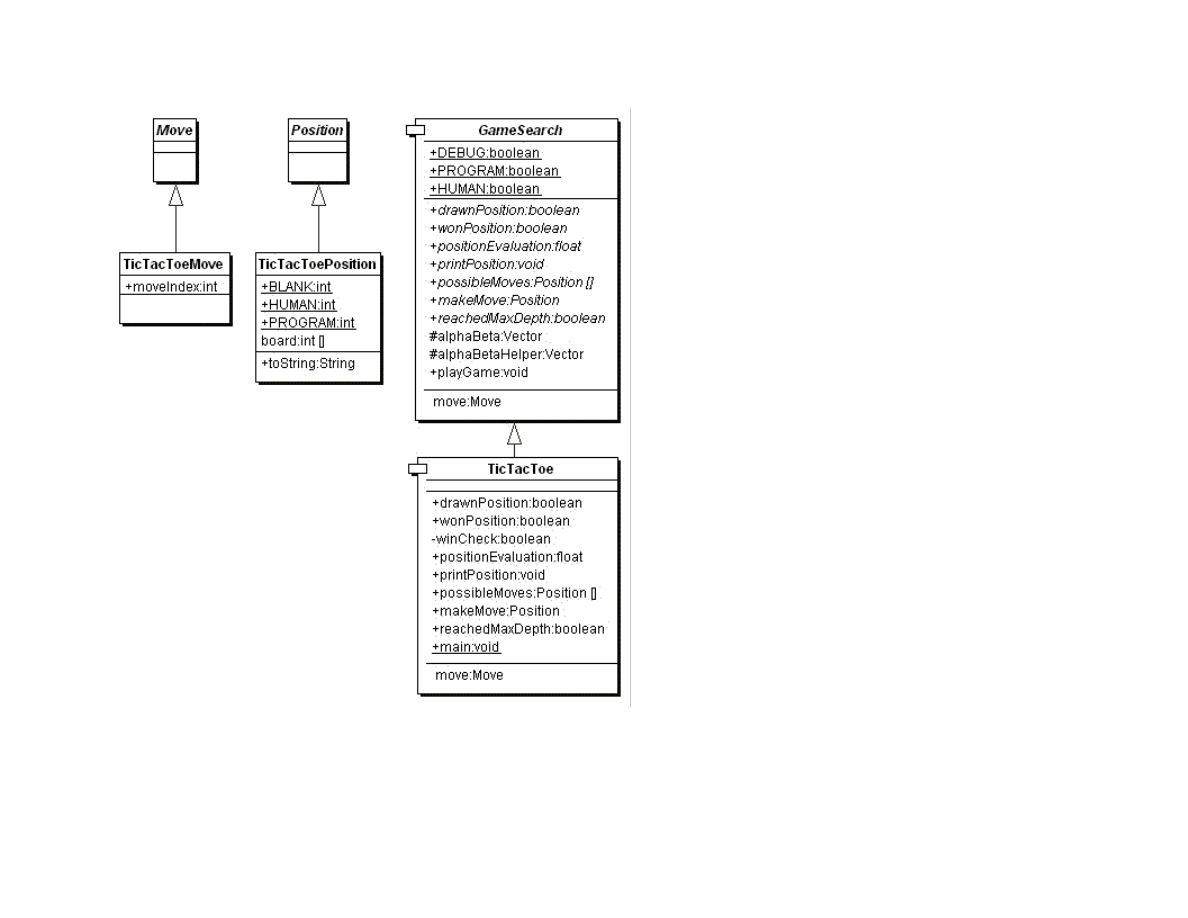
30
Figure 1.9 UML class diagrams for game search engine and tic-tac-toe
I assume that the reader has the code from my web site installed and available for viewing. In this section, I will only discuss the most
interesting details of the tic-tac-toe class refinements; I assume that the reader can look at the source code. We will start by looking at
the refinements for the position and move classes. The TicTacToeMove class is trivial, adding a single integer value to record the
square index for the new move:
public class TicTacToeMove extends Move {

31
public int moveIndex;
}
The board position indices are in the range of [0..8] and can be considered to be in the following order:
0 1 2
3 4 5
6 7 8
The class TicTacToePosition is also simple:
public class TicTacToePosition extends Position {
final static public int BLANK = 0;
final static public int HUMAN = 1;
final static public int PROGRAM = -1;
int [] board = new int[9];
public String toString() {
StringBuffer sb = new StringBuffer("[");
for (int i=0; i<9; i++) sb.append(""+board[i]+",");
sb.append("]");
return sb.toString();
}
}
This class allocates an array of nine integers to represent the board, defines constant values for blank, human, and computer squares,
and defines a toString method to print out the board representation to a string.
The TicTacToe class must define the following abstract methods from the base class GameSearch:
public abstract boolean drawnPosition(Position p)
public abstract boolean wonPosition(Position p, boolean player)
public abstract float positionEvaluation(Position p,
boolean player)
public abstract void printPosition(Position p)
public abstract Position [] possibleMoves(Position p,
boolean player)
public abstract Position makeMove(Position p, boolean player,
Move move)
public abstract boolean reachedMaxDepth(Position p, int depth)
public abstract Move getMove()
The implementation of these methods uses the refined classes TcTacToeMove and TicTacToePosition. For example, consider the
class drawnPosition that is responsible for selecting a drawn (or tied) position:
public boolean drawnPosition(Position p) {

32
boolean ret = true;
TicTacToePosition pos = (TicTacToePosition)p;
for (int i=0; i<9; i++) {
if (pos.board[i] == TicTacToePosition.BLANK){
ret = false;
break;
}
}
return ret;
}
The methods that are overridden from the GameSearch base class must always cast arguments of type Position and Move to
TicTacToePosition and TicTacToeMove. Note that in the method drawnPosition, the argument of class Position is cast to the class
TicTacToePosition. A position is considered to be a draw if all of the squares are full. We will see that checks for a won position are
always made before checks for a drawn position, to that the method drawnPosition does not need to make a redundant check for a
won position. The method wonPosition is also simple; it uses a private helper method winCheck to test for all possible winning
patterns in tic-tac-toe. The method positionEvaluation uses the following board features to assign a fitness value from the point of
view of either player:
The number of blank squares on the board
If the position is won by either side
If the center square is taken
The method positionEvaluation is simple, and is a good place for the interested reader to start modifying both the tic-tac-toe and
chess programs:
public float positionEvaluation(Position p, boolean player) {
int count = 0;
TicTacToePosition pos = (TicTacToePosition)p;
for (int i=0; i<9; i++) {
if (pos.board[i] == 0) count++;
}
count = 10 - count;
// prefer the center square:
float base = 1.0f;
if (pos.board[4] == TicTacToePosition.HUMAN &&
player) {
base += 0.4f;
}
if (pos.board[4] == TicTacToePosition.PROGRAM &&
!player) {
base -= 0.4f;
}
float ret = (base - 1.0f);
if (wonPosition(p, player)) {

33
return base + (1.0f / count);
}
if (wonPosition(p, !player)) {
return -(base + (1.0f / count));
}
return ret;
}
The only other method that we will look at here is possibleMoves; the interested reader can look at the implementation of the other
(very simple) methods in the source code. The method possibleMoves is called with a current position, and the side to move (i.e.,
program or human):
public Position [] possibleMoves(Position p, boolean player)
{
TicTacToePosition pos = (TicTacToePosition)p;
int count = 0;
for (int i=0; i<9; i++) if (pos.board[i] == 0) count++;
if (count == 0) return null;
Position [] ret = new Position[count];
count = 0;
for (int i=0; i<9; i++) {
if (pos.board[i] == 0) {
TicTacToePosition pos2 =
new TicTacToePosition();
for (int j=0; j<9; j++)
pos2.board[j] = pos.board[j];
if (player) pos2.board[i] = 1;
else pos2.board[i] = -1;
ret[count++] = pos2;
}
}
return ret;
}
It is very simple to generate possible moves: every blank square is a legal move. (This method will not be as simple in the example
chess program!)
It is simple to compile and run the example tic-tac-toe program: change directory to src/search/game and type:
javac *.java
java TicTacToe
When asked to enter moves, enter an integer between 0 and 8 for a square that is currently blank (i.e., has a zero value). The following
shows this labeling of squares on the tic-tac-toe board:

34
0 1 2
3 4 5
6 7 8
1.5.4 Chess using the alpha beta search algorithm
Using the Java class framework of GameSearch, Position, and Move, it is reasonably simple to write a simple chess program by
writing three new derived classes (see Figure 1.10) Chess (derived from GameSearch), ChessMove (derived from Move), and
ChessPosition (derived from Position). The chess program developed in this section is intended to be an easy to understand example
of using alpha-beta min-max search; as such, it ignores several details that a fully implemented chess program would implement:
Allow the computer to play either side (computer always plays black in this example)
Allow en-passant pawn captures.
Allow the player to take back a move after making a mistake
The reader is assumed to have read the last section on implementing the tic-tac-toe game; details of refining the GameSearch, Move,
and Position classes are not repeated in this section.
Figure 1.10 shows the UML class diagram for both the general purpose GameSearch framework and the classes derived to implement
chess specific data and behavior.
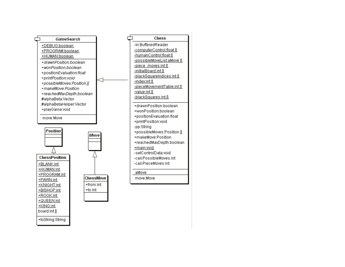
35
Figure 1.10 UML class diagrams for game search engine and chess
The class ChessMove contains data for recording from and to square indices:

36
public class ChessMove extends Move {
public int from;
public int to;
}
The board is represented as an integer array with 120 elements. A chessboard only has 64 squares; the remaining board values are set
to a special value of 7, which indicates an “off board” square. The initial board setup is defined statically in the Chess class:
private static int [] initialBoard = {
7, 7, 7, 7, 7, 7, 7, 7, 7, 7, 7,
7, 7, 7, 7, 7, 7, 7, 7, 7, 7, 7,
4, 2, 3, 5, 9, 3, 2, 4, 7, 7, // white pieces
1, 1, 1, 1, 1, 1, 1, 1, 7, 7, // white pawns
0, 0, 0, 0, 0, 0, 0, 0, 7, 7, // 8 blank squares, 2 off board
0, 0, 0, 0, 0, 0, 0, 0, 7, 7, // 8 blank squares, 2 off board
0, 0, 0, 0, 0, 0, 0, 0, 7, 7, // 8 blank squares, 2 off board
0, 0, 0, 0, 0, 0, 0, 0, 7, 7, // 8 blank squares, 2 off board
-1,-1,-1,-1,-1,-1,-1,-1, 7, 7, // black pawns
-4,-2,-3,-5,-9,-3,-2,-4, 7, 7, // black pieces
7, 7, 7, 7, 7, 7, 7, 7, 7, 7, 7,
7, 7, 7, 7, 7, 7, 7, 7, 7, 7, 7
};
The class ChessPosition contains data for this representation and defines constant values for playing sides and piece types:
public class ChessPosition extends Position {
final static public int BLANK = 0;
final static public int HUMAN = 1;
final static public int PROGRAM = -1;
final static public int PAWN = 1;
final static public int KNIGHT = 2;
final static public int BISHOP = 3;
final static public int ROOK = 4;
final static public int QUEEN = 5;
final static public int KING = 6;
int [] board = new int[120];
public String toString() {
StringBuffer sb = new StringBuffer("[");
for (int i=22; i<100; i++) {
sb.append(""+board[i]+",");
}
sb.append("]");
return sb.toString();
}
}

37
The class Chess also defines other static data. The following array is used to encode the values assigned to each piece type (e.g.,
pawns are worth one point, knights and bishops are worth 3 points, etc.):
private static int [] value = {
0, 1, 3, 3, 5, 9, 0, 0, 0, 12
};
The following array is used to codify the possible incremental moves for pieces:
private static int [] pieceMovementTable = {
0, -1, 1, 10, -10, 0, -1, 1, 10, -10, -9, -11, 9,
11, 0, 8, -8, 12, -12, 19, -19, 21, -21, 0, 10, 20,
0, 0, 0, 0, 0, 0, 0, 0
};
The starting index into the pieceMovementTable array is calculated by indexing the following array with the piece type index (e.g.,
pawns are piece type 1, knights are piece type 2, bishops are piece type 3, rooks are piece type 4, etc.:
private static int [] index = {
0, 12, 15, 10, 1, 6, 0, 0, 0, 6
};
When we implement the method possibleMoves for the class Chess, we will see that, except for pawn moves, that all other possible
piece type moves are very simple to calculate using this static data. The method possibleMoves is simple because it uses a private
helper method calcPieceMoves to do the real work. The method possibleMoves calculates all possible moves for a given board
position and side to move by calling calcPieceMove for each square index that references a piece for the side to move.
We need to perform similar actions for calculating possible moves and squares that are controlled by each side. In the first version of
the class Chess that I wrote, I used a single method for calculating both possible move squares and controlled squares. However, the
code was difficult to read, so I split this initial move generating method out into three methods:
possibleMoves – required because this was an abstract method in GameSearch. This method calls calcPieceMoves for all squares
containing pieces for the side to move, and collects all possible moves.
calcPieceMoves – responsible to calculating pawn moves and other piece type moves for a specified square index.
setControlData – sets the global array computerControl and humanControl. This method is similar to a combination of
possibleMoves and calcPieceMoves, but takes into effect “moves” onto squares that belong to the same side for calculating the
effect of one piece guarding another. This control data is used in the board position evaluation method positionEvaluation.
We will discuss calcPieceMoves here, and leave it as an exercise to carefully read the similar method setControlData in the source
code. This method places the calculated piece movement data in static storage (the array piece_moves) to avoid creating a new Java

38
object whenever this method is called; method calcPieceMoves returns an integer count of the number of items placed in the static
array piece_moves. The method calcPieceMoves is called with a position and a square index; first, the piece type and side are
determined for the square index:
private int calcPieceMoves(ChessPosition pos,
int square_index) {
int [] b = pos.board;
int piece = b[square_index];
int piece_type = piece;
if (piece_type < 0) piece_type = -piece_type;
int piece_index = index[piece_type];
int move_index = pieceMovementTable[piece_index];
if (piece < 0) side_index = -1;
else side_index = 1;
Then, a switch statement controls move generation for each type of chess piece (movement generation code is not shown):
switch (piece_type) {
case ChessPosition.PAWN:
break;
case ChessPosition.KNIGHT:
case ChessPosition.BISHOP:
case ChessPosition.ROOK:
case ChessPosition.KING:
case ChessPosition.QUEEN:
break;
}
The logic for pawn moves is a little complex but the implementation is simple. We start by checking for pawn captures of pieces of the
opposite color. Then check for initial pawn moves of two squares forward, and finally, normal pawn moves of one square forward.
Generated possible moves are placed in the static array piece_moves and a possible move count is incremented. The move logic for
knights, bishops, rooks, queens, and kings is very simple since it is all table driven. First, we use the piece type as an index into the
static array index; this value is then used as an index into the static array pieceMovementTable. There are two loops: an outer loop
fetches the next piece movement delta from the pieceMovementTable array and the inner loop applies the piece movement delta set
in the outer loop until the new square index is off the board or “runs into” a piece on the same side. Note that for kings and knights,
the inner loop is only executed one time per iteration through the outer loop:
move_index = piece;
if (move_index < 0) move_index = -move_index;
move_index = index[move_index];
//System.out.println("move_index="+move_index);
next_square = square_index + pieceMovementTable[move_index];
outer:
while (true) {

39
inner:
while (true) {
if (next_square > 99) break inner;
if (next_square < 22) break inner;
if (b[next_square] == 7) break inner;
// check for piece on the same side:
if (side_index < 0 && b[next_square] < 0)
break inner;
if (side_index >0 && b[next_square] > 0)
break inner;
piece_moves[count++] = next_square;
if (b[next_square] != 0) break inner;
if (piece_type == ChessPosition.KNIGHT)
break inner;
if (piece_type == ChessPosition.KING) break inner;
next_square += pieceMovementTable[move_index];
}
move_index += 1;
if (pieceMovementTable[move_index] == 0) break outer;
next_square = square_index +
pieceMovementTable[move_index];
}
The method setControlData is very similar to this method; leave it as an exercise to the reader to read through the source code.
Method setControlData differs in also considering moves that protect pieces of the same color; calculated square control data is
stored in the static arrays computerControl and humanControl. This square control data is used in the method positionEvaluation
that assigns a numerical rating to a specified chessboard position or either the computer or human side. The following aspects of a
chessboard position are used for the evaluation:
material count (pawns count 1 point, knights and bishops 3 points, etc.)
count of which squares are controlled by each side
extra credit for control of the center of the board
credit for attacked enemy pieces
Notice that the evaluation is calculated initially assuming the computer’s side to move; if the position if evaluated from the human
player’s perspective, the evaluation value is multiplied by minus one. The implementation of positionEvaluation is:
public float positionEvaluation(Position p, boolean player) {
ChessPosition pos = (ChessPosition)p;
int [] b = pos.board;
float ret = 0.0f;
// adjust for material:

40
for (int i=22; i<100; i++) {
if (b[i] != 0 && b[i] != 7) ret += b[i];
}
// adjust for positional advantages:
setControlData(pos);
int control = 0;
for (int i=22; i<100; i++) {
control += humanControl[i];
control -= computerControl[i];
}
// Count center squares extra:
control += humanControl[55] - computerControl[55];
control += humanControl[56] - computerControl[56];
control += humanControl[65] - computerControl[65];
control += humanControl[66] - computerControl[66];
control /= 10.0f;
ret += control;
// credit for attacked pieces:
for (int i=22; i<100; i++) {
if (b[i] == 0 || b[i] == 7) continue;
if (b[i] < 0) {
if (humanControl[i] > computerControl[i]) {
ret += 0.9f * value[-b[i]];
}
}
if (b[i] > 0) {
if (humanControl[i] < computerControl[i]) {
ret -= 0.9f * value[b[i]];
}
}
}
// adjust if computer side to move:
if (!player) ret = -ret;
return ret;
}
It is simple to compile and run the example chess program: change directory to src/search/game and type:
javac *.java
java Chess
When asked to enter moves, enter string like “d2d4” to enter a move in chess algebraic notation. Here is sample output from the
program:
Board position:
41
BR BN BB . BK BB BN BR
BP BP BP BP . BP BP BP
. . BP BQ .
. . . .
. WP . .
. . . WN .
WP WP WP . WP WP WP WP
WR WN WB WQ WK WB . WR
Your move:
c2c4
The example chess program plays, in general good moves, but its play could be greatly enhanced with an “opening book” of common
chess opening move sequences. If you run the example chess program, depending on the speed of your computer and your Java
runtime system, the program takes a while to move (about 15 seconds per move on my PC). Where is the time spent in the chess
program? Table 1.1 shows the total runtime (i.e., time for a method and recursively all called methods) and method-only time for the
most time consuming methods. Methods that show zero percent method only time used less that 0.1 percent of the time so they print
as zero values.
Table 1.1
Class.method name
Percent of total runtime Percent in this method
only
Chess.main
97.7
0.0
GameSearch.playGame
96.5
0.0
GameSearch.alphaBeta
82.6
0.0
GameSearch.alphaBetaHelper 82.6
0.0
Chess.positionEvaluate
42.9
13.9
Chess.setControlData
29.1
29.1
Chess.possibleMoves
23.2
11.3
Chess.calcPossibleMoves
1.7
0.8
Chess.calcPieceMoves
1.7
0.8
The interested reader is encouraged to choose a simple two-player game, and using the game search class framework, implement your
own game-playing program.

42
Chapter 2. Natural Language Processing
Human understanding of language requires background or common sense knowledge of the world. Human consciousness is tightly
coupled with both language and our internal models of the outer world. Indeed, many (e.g., [Capra 1966]) argue that it is our
consciousness that creates our own world (i.e., we create the worlds that we live in). I think that it is likely that the most accurate
model of consciousness (human or otherwise) requires that the effect of consciousness on the external world is important; it makes
little sense to assume that the real world is static and is not affected by conscious entities living in that world.
So, in trying to understand life and consciousness, it is important to understand the context of experiences in the world. Children
playing often make up new words spontaneously that for the children involved has real meaning in the context of their lives. Where
does this leave us if we want to write software for Natural Language Processing (NLP)? There are two basic approaches depending on
whether we want to write an effective “natural language front end” to a software system (e.g., a query system for a database, which we
will do in this chapter) or if we are motivated to do fundamental research on minds and consciousness by building a system that
acquires structure and intelligence through its interaction with its environment (e.g., the Magnus system [Aleksander, 1996]).
We will look at parsing techniques in this chapter. Historically, most NLP work has been has used parsers that combine a grammar
with a lexicon to produce the structure of sentences. In Chapter 7, we will look at an alternative approach to NLP: using statistical
algorythms to assign word type tags to words in sentences.
The examples for this chapter are found in the subdirectory src in:
src
src/nlp
src/nlp/ATN – ATN parser that uses data from Wordnet (Wordnet data must be downloaded separately – see the Readme.txt file)
src/nlpNLBean – my Open Source natural language database interface
src/nlp/prolog – NLP using embedded Prolog
src/prolog – source code for Prolog engine written by Sieuwert van Otterloo
There are several common techniques for practical NLP systems:
Finite state machines that recognize word sequences as syntactically valid sentence (often called augmented transition networks, or
ATNs). These state machines are often written in Prolog, LISP, or C.
Conceptual dependency parsers that stress semantics rather than syntax. These are usually written in LISP. Conceptual
Dependency is an old technique that is not used much anymore.
Statistical natural language techniques (covered in Chapter 7)

43
This chapter uses three example systems:
An ATN based parser using parts of the Wordnet 1.6 lexicon
An existing Open Source system written by the author for accessing relational databases with simple natural language queries.
This example uses information from the databases (e.g., table and column names) in parsing natural language and producing valid
SQL database queries.
A parser written in Prolog, with an example of using this parser in a Java application
Advertisement
KnowledgeBooks.com and MarkWatson.com - industrial strength NLP tools. KnowledgeBooks.com is a privately held company
owned by the author and MarkWatson.com is the author’s consulting company.
2.1 ATN Parsers
ATN parsers are finite state machines that recognize word sequences as specific words, noun phrases, verb phrases, etc. The original
work done on ATNs was done by W. A. Woods in the late 1960s to address a shortcoming of context free grammars for NLP, which
include:
Difficulty in dealing with different sentence structures that has the same meanings. Typically, the grammar has to be expanded to
handle many special cases.
Handling number agreement between subjects and verbs.
Determining the “deep structure” of input texts.
The term morphological tags (or features) refers to the labeling of words with part of speech tags; for example:
Noun – cat, dog, boy, etc.
Pronouns – he, she, it
Relative pronouns – which, who, that
Verb – run, throw, see, etc.

44
Determiners
Articles – a, an, the
Possessives – my, your, theirs, etc.
Demonstratives – this, that, these, those
Numbers
Adjectives – big, small, purple, etc.
Adverbs
Describe how something is done – fast, well, etc.
Time – after, soon, etc.
Questioning – how, why, when, where
Place – down, up, here, etc.
In general, accurately assigning correct morphological tags (i.e., parts of speech) to input text is a difficult problem, as we will see
when we build an ATN parser. There are other good techniques for assigning word types, like Hidden Markov Model and Bayesian
techniques (web search “part of speech tagging Bayesian”). One problem with assigning parts of speech is that a given word can be
used in many ways; for example, bank (noun, verb, adjective). English grammar is complex! The important steps in building NLP
technology into your own programs are:
Reduce the domain of discourse (i.e., what the system can “understand”) to a minimum
Create a set of “use cases” to focus your effort in designing and writing ATNs, and to use for testing your NLP system during
development
When possible, capture text input from real users of your system, and incrementally build up a set of “use cases” that your system can
handle correctly
Map identified words/parts of speech to actions that your system should perform (e.g., see the data base query system developed at the
end of this chapter)
ATN parsers can be represented graphically, with different graph structures for handling complete sentences, noun phrases, verb
phrases, etc. We will look at a very simple example in Figure 2.1.
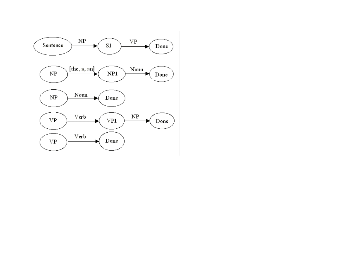
45
Figure 2.1 A simplified ATNs for handling a few cases of noun and verb phrases
We will parse a simple example using the ATNs in Figure 2.1 so you get a feeling for how ATN-based parsers work. ATNs in Figure
2.1 are always evaluated from top to bottom; it is common to evaluate more complex ATNs of the same type before simpler ones. For
example, we always test the more complex NP ATN in Figure 2.1 before trying the simpler one. As a first example, consider the
sentence “a dog ran”. We street any input text as being an ordered sequence of words, in this case [a, dog, ran]. The arrows in Figure
2.1 represent tests that must be passed before proceeding to the next node in the ATN. If the sequence [a, dog, ran] is input to the top
level Sentence node, in order to pass the first test, the ATN NP must accept the word or words at the beginning of this sequence. The
first test to transition between NP and NP1 is a test to see if the first word in the sequence is in the set [the, a, and]. This test is
passed, so the word or words that satisfied the test are removed from the input sequence. In order to transition between the node NP1
and the Done node, the next remaining word in the input sequence must be a noun, which it is; so, the word dog is removed from the
input sequence, and we are done with the NP ATN, returning the shortened input sequence to node S1 of the top level Sentence ATN.
In order to transition from node S1 to the Done node, the shortened input sequence [ran] must pass the VP ATN test. We can
transition from node VP to node VP1 because the first word in the input sequence [ran] is a verb. However, we cannot transition from
node VP1 to the Done node because there are no remaining words in the input sequence. Not a problem; we return from the first VP
ATN, restoring the input sequence to the state that it was in when we entered the ATN, in this case [ran]. Now, we try the simpler VP

46
ATN at the bottom of Figure 2.1, and we can successfully transition from the VP node to the Done node because the first word in the
input sequence is a verb. This allows us to return to the calling Sentence ATN and transition to the Done node.
In this example, the individual ATNs might have been augmented to contain code and data to remember words that appeared in a
specific context. For example, the noun that helped pass the NP test could be saved. However, this example is actually a Recursive
Transition Network because it has not been augmented. We will see that it is fairly easy to augment the code for recognizing individual
ATNs to save word values. In Woods original system, he used the term registers to indicate the memory used to, for example,
remember the leading noun in a noun phrase (see the NP ATNs in Figure 2.1).
In the Java example that we will shortly write, the example ATN program has placeholder code that can be used to remember specific
words while processing ATNs. Also, we use many ATNs, always trying more complex ATNs of the same type before the simpler ones.
The ATNs in Figure 2.1 implement the following pattern:
NP -> VP
A short list of the ATN patterns (taken from the Java example source code) that we will use is seen in Listing 2.1.
Listing 2.1
int [] ALL_S [] = {
{NP, VP, NP, PP, VP},
{NP, VP, PP, NP},
{NP, VP, NP},
{VP, NP, PP, NP},
{VP, PP, NP},
{NP, VP}, // this one matches Figure 2.1
{VP, PP},
{VP, NP},
{VP}
};
We will write Java methods to recognize if word sequences satisfying the NP, VP, and PP tests. PP stands for prepositional phrase.
Parsing using ATN networks is a depth first search process. In our example system, this search process will halt as soon as an input
word sequence is recognized; this is the reason that we check the most complex ATNs first.
2.1.1 Lexicon data for defining word types

47
In the example in Figure 2.1, we assumed that we could tell if a word was a noun, verb, etc. In order to meet this requirement in the
example system, we will build a lexicon that indicates word types for many common words. For example, lexicon entries might look
like:
book – noun, verb (e.g., “I want to book a flight”)
run – noun (e.g., “did you hit in a run?”), verb, adjective (e.g., “you look run down”)
We will use the Wordnet lexical database to build a lexicon. The Wordnet lexical database from Princeton University is one of the
most valuable tools available for experimenting with NLP systems. The full Wordnet system contains information on “synsets” of
collection of synonyms and example uses for most commonly used English words. Wordnet data files comprise index and separate
data files. We use the index files for the word types noun, verb, adjective and adverb. Additional words are added for the word types
articles, conjunctions, determiners, prepositions, and pronouns in the Java ATN parser class that will be designed and implemented
later in this chapter. The Wordnet synset data is not used in the example ATN system.
2.1.2 Design and implementation of an ATN parser in Java
The example ATN parsing system consists of two Java classes, the original Wordnet index files, and a serialized Java object file
containing hash tables for the word types noun, verb, adjective and adverb. The ZIP file for this book contains the serialized data file,
but not the original Wordnet data files; the interested reader will find a link to the Wordnet web site on the support web page for this
book.
New: I no longer distribute a pre-built lexicon file because it greatly increased the download size of this web book. Please follow the
directions in src/nlp/ATN/Readme.txt for building the file wncache.dat. Figure 2.1 shows the Java classes for the utility class
MakeWordnetCache and the ATN example program.

48

49
Figure 2.2 ATN and MakeWordnetCache UML class diagrams.
Both the MakeWordnetCache and ATN Java classes show a very useful technique: preprocessing data required by an executing Java
program, and saving it as a serialized object. The MakeWordnetCache program is fairly simple, basically using the method
helper(String file, Hashtable hash) to read a Wordnet index file and fill in each word in the provided hash table. It is worth taking a
quick look at the code to serialize the four generated hash tables into a file:
try {
FileOutputStream ostream = new FileOutputStream("wncache.dat");
ObjectOutputStream p = new ObjectOutputStream(ostream);
p.writeObject(adj); // adj is a hash table
p.writeObject(adv); // adv is a hash table
p.writeObject(noun); // noun is a hash table
p.writeObject(verb); // verb is a hash table
p.flush();
ostream.close();
} catch (Exception e) {
e.printStackTrace();
}
The code in the ATN class constructor will either read the file wncache.dat from the local directory, or if the compiled ATN class and
the wncache.dat files are delivered in a JAR archive file, the wncache.dat data file will be automatically read from the JAR file. This
is a very useful technique so let’s take a quick look at the code that reads a data file from either the current directory or a JAR archive
that is in the CLASSPATH used when running the ATN program:
try {
// the following code will read either a local file of a
// resource in a JAR file:
InputStream ins =
ClassLoader.getSystemResourceAsStream("wncache.dat");
if (ins==null) {
System.out.println("Failed to open 'wncache.dat'");
System.exit(1);
} else {
ObjectInputStream p = new ObjectInputStream(ins);
adj = (Hashtable)p.readObject();
adv = (Hashtable)p.readObject();
noun = (Hashtable)p.readObject();
verb = (Hashtable)p.readObject();
ins.close();
}
}
If you wanted to package the ATN example for someone, you could make a JAR file by using the following commands:

50
jar cvf atn.jar ATN.class wncache.dat
erase *.class
erase wncache.dat
You could then run the system, using only the jar file, by using:
java –classpath atn.jar ATN “the dog ran down the street”
Processing : the dog ran down the street
'the' possible word types: art
'dog' possible word types: noun verb
'ran' possible word types: verb
'down' possible word types: adj adv noun prep verb
'the' possible word types: art
'street' possible word types: noun
Best ATN at word_index 0
word: the part of speech: art
word: dog part of speech: noun
word: ran part of speech: verb
word: down part of speech: adj
word: the part of speech: art
word: street part of speech: noun
The primary class methods for ATN are:
ATN – class constructor reads hash tables for noun, verb, adverb, and adjective from a serialized data file and then creates smaller
has tables for handling articles, conjunctions, determiners, pronouns, and prepositions.
addWords – private helper method called by the class constructor to add an array of strings to a specified hash table
checkWord – checks to see is a given word is of a specified word type
parse – public method that handles parsing a sequence of words stored in a single Java string. The words are copied to an array of
strings one word per string); this array is a class variable words. Then the helper function parse_it is called to test the word
sequence in the array words against all ATN test in the class variable ALL_S. The ATN test that parses the most words in the input
word sequence is then used.
parse_it – uses the ATN test method parseSentence to run all of the ATN tests. Note that parseSentance and all of the other ATN
implementation methods take an integer argument hat is an index into the class array words.
parseSentence – evaluates all ATN tests seen in Listing 2.1 to see which one parses the most words in the input word sequence.
The private method parseHelper is called with each array element of the array ALL_S.
parseHelper – uses the ATN implementation methods parseNP, parseVP, and parsePP to evaluate one of the test ATNs in the global
array ALL_S. The return value is the number of words in the original input word sequence that this particular test ATN recognized.

51
The ATN implementation methods parseNP, parseVP, and parsePP all use the same process that we used in Section 2.1 to manually
process the word sequence [a, dog, ran] using the simple test ATNs in Figure 2.1. We will look at one of these methods, parseNP, in
detail; the others work in a similar way. The following listing shows parts of the method parseNP with comments:
The method parseNP has two arguments, the starting word index in the array words, and an offset from this starting word index:
int parseNP(int start_word_index, int word_index) {
We first check to make sure that there is still work to do:
if (word_index >= num_words) return word_index;
The following code tests for the pattern of a noun followed by a conjunction, followed by another noun phrase:
// test ATN transitions <NOUN> --> <CONJ> --> <NP>
if (word_index < num_words - 2 &&
checkWord(words[word_index], NOUN))
{
if (checkWord(words[word_index + 1], CONJ)) {
int ii = parseNP(start_word_index, word_index + 2);
if (ii > -1) {
partsOfSpeech[start_word_index + word_index] = NOUN;
partsOfSpeech[start_word_index + word_index + 1]
= CONJ;
return ii;
}
}
}
In this code, it is necessary to first check to see if there are sufficient words to process, then we test for a noun/conjunction pair, then
recursively call parseNP again for the word sequence occurring after the noun and conjunction. If this last recursive call tests out OK,
then we set the word types of the noun and conjunction, and return with the index of the word in the input sequence following the last
word in the recognized noun phrase.
The next test, for an article followed by another noun phrase, is similar, except we only need to check for one extra word past the
current word index:
// test ATN transitions <ART> --> <NP>
if (word_index < num_words - 1 &&
checkWord(words[word_index], ART))
{
int ii = parseNP(start_word_index, word_index + 1);
if (ii > -1) {

52
partsOfSpeech[start_word_index + word_index] = ART;
return ii;
}
}
The next test is different because we do not recursively call parseNP. Instead, we just check for two nouns together at the beginning
of the tested word sequence:
// test ATN transitions <NOUN> --> <NOUN>
if (word_index < num_words - 1 &&
checkWord(words[word_index], NOUN))
{
if (checkWord(words[word_index + 1], NOUN)) {
partsOfSpeech[start_word_index + word_index] = NOUN;
partsOfSpeech[start_word_index + word_index + 1] = NOUN;
return word_index + 2;
}
}
The next check is even simpler (remember, we favor the more complex tests by evaluating them first); here we simply check to see if
the next word is a noun, and if it is, we recognize a noun phrase, returning the word index following the noun:
if (checkWord(words[word_index], NOUN)) {
partsOfSpeech[start_word_index + word_index] = NOUN;
return word_index + 1;
}
In the next test, we accept a pronoun followed by another noun phrase. As before, we use a recursive call to parseNP:
if (checkWord(words[word_index], PRON)) {
int ii = parseNP(start_word_index, word_index + 1);
if (ii > -1) {
partsOfSpeech[start_word_index + word_index] = PRON;
return ii;
}
}
The final test that we perform, if required, I to check to see if the next word in the input sequence is a pronoun: if it is, we accept the
current sequence as a noun phrase and return in the index of the word following the pronoun:
if (checkWord(words[word_index], PRON)) {
partsOfSpeech[start_word_index + word_index] = PRON;
return word_index + 1;
}

53
If all of the above tests fail, we return the value of minus one as a flag to the parseHelper method that this ATN test failed.
return -1;
The other built in methods for ATN tests like parseVP and parsePP are similar to parseNP, and we will not review the code for them.
2.1.3 Testing the Java ATN parser
The main method of the class ATN will parse the word sequence “the dog ran down the street” if no command line arguments are
supplied. Otherwise, each command line argument is considered to be a string and the words in each input string are parsed in order.
For example:
java ATN “the cat sees the dog” “I like to see a movie”
Processing : the cat sees the dog
'the' possible word types: art
'cat' possible word types: noun verb
'sees' possible word types:
'the' possible word types: art
'dog' possible word types: noun verb
Best ATN at word_index 0
word: the part of speech: art
word: cat part of speech: noun
word: sees part of speech: verb
word: the part of speech: art
word: dog part of speech: noun
Processing : I like to see a movie
'i' possible word types: adj noun
'like' possible word types: adj verb
'to' possible word types: prep
'see' possible word types: adv noun verb
'a' possible word types: art noun
'movie' possible word types: noun
Best ATN at word_index 0
word: i part of speech: noun
word: like part of speech: verb
word: to part of speech: prep
word: see part of speech: adv
word: a part of speech: art
word: movie part of speech: noun

54
One thing that you will notice when you experiment with this ATN parser: it sometimes incorrectly identifies the part of speech for
one or more words in the input word sequence. It is important, when using NLP in your programs, to identify a set of test sentences
that might be typically used in running you application, and you will need to modify the parser in two ways to tailor it for your
application:
Change the top level ATN tests shown in Listing 2.1
Change some of the built in ATN test methods like parseNP and parseVP
We will see an example of an NLP system in the next section that has been tailored to one specific domain: querying a database when
we know the meta data (e.g., column names and database names) for a database.
2.2 Using Prolog for NLP
This section is the second time in this book that we use the declarative nature of Prolog to solve a problem in a more natural notation
than we could in procedural Java code. If the reader has had no exposure to Prolog, I suggest doing a web search for “Prolog logic
tutorial”. We used ATN parsers at the beginning of this chapter; ATNs are procedural, so an implementation in Java made sense. In this
section, we will see how effective Prolog is for NLP. If this short treatment of NLP in Prolog whets the readers appetite, a web search
for “Prolog NLP” will provide access to a huge body of work; the interested reader can use the techniques for using the pure Java
Prolog Engine (written by Sieuwert van Otterloo) in her own programs.
2.2.1 Prolog examples of parsing simple English sentences
We will start by using Prolog to recognize a subset of English sentences. Consider the following Prolog rules (excerpts from the file
src/nlp/prolog/p0.pl):
The following Prolog rule can recognize a noun phrase:
noun_phrase([D,N]) :-
determiner(D),
noun(N).
noun_phrase([N]) :-
noun(N).

55
The first rule states that we can return a list [D,N] if D is a determiner and N is a noun. The second rule states that we can return a list
[N] if N is a noun.
If we can test this with:
?- noun_phrase([the,dog]).
yes.
Here, I am using a standalone Prolog system. The “?-“ is a prompt for a query, and the response “yes” means that the list [the,dog] was
recognized as a noun phrase. The list [the, throws] will not be recognized as a noun phrase:
?- noun_phrase([the, throws]).
no.
We can recognize word types using the Prolog member rule and a list of words of a desired type; for example:
determiner(D) :-
member(D,[the,a,an]).
noun(N) :-
member(N,[dog, street, ball, bat, boy]).
verb(V) :-
member(V,[ran, caught, yelled, see, saw]).
A rule for recognizing a complete sentence might look like:
sentence(S) :-
noun_phrase(NP),
verb_phrase(VP),
append(NP,VP,S).
This rule uses a standard Prolog technique: for recognizing lists like [the,dog, ran] or [the,dog, ran, down, the, street], we do not know
how many words will be in the noun phrase and how many will be in the verb phrase. Here, the Prolog rule append comes to the
rescue: using backtrack search, the append rule will cycle through the permutations of splitting up a list into two parts, one sub list for
NP and one sub list for VP. We now can recognize a sentence:
?- sentence([the,dog, ran, down, the, street]).
yes.
This is fine for a demonstration of how simple it is to use Prolog to recognize a subset of English sentences, but it does not give us the
structure of the sentence. The example file p.pl is very similar to the last example file p0.pl, but each rule is augmented to store the
structure of the words being parsed. The following code fragments show part of the example file p.pl:

56
We will start be looking at the modifications required for storing the parsed sentence structure for two of the rules. Here is the original
example for testing to see if a word is a determiner:
determiner(D) :-
member(D,[the,a,an]).
Here are the changes for saving the struture after a determiner word has been recognized:
determiner([D],determiner(D) ) :-
member(D,[the,a,an]).
We will test this to show how the structure appears:
?-determiner([a],D).
D=determiner(a)
yes.
If we look at a more complex rule that uses the determiner rule, you can see how the structure is built from sub lists:
noun_phrase(NP,noun_phrase(DTree,NTree)) :-
append(D,N,NP),
determiner(D,DTree),
noun(N,NTree).
Again, we will test this new rule to see how the structure is built up:
?- noun_phrase([a,street], NP).
NP=noun_phrase(determiner(a),noun(street))
yes.
Skipping some of the rules defined in the file p.pl, here is the top level parsing rule to recognize and produce the structure of a simple
sentence:
sentence(S, sentence(NPTree,VPTree) ) :-
append(NP,VP,S),
noun_phrase(NP,NPTree),
verb_phrase(VP,VPTree).
Here, we use the built in append rule to generate permutations of dividing the list S into two sub lists NP and VP, and the rules for
recognizing and building structures for noun and verb phrases. To demonstrate how the append rule works, we will use it to slice up a
short sentence (note: we type “
;
” after Prolog prints a matchto try to get additional matches):

57
?- append(NP,VP,[the,dog,ran]).
NP=[]
VP=[the,dog,ran]
;
NP=[the]
VP=[dog,ran]
;
NP=[the,dog]
VP=[ran]
;
NP=[the,dog,ran]
VP=[]
;
Here is a final example of parsing and building the structure for a longer sentence:
?- sentence([the,dog,ran,down,the,strret],S).
S=sentence(noun_phrase(determiner(the),noun(dog)),verb_phrase(verb(ran)))
yes.
This could be “pretty printed” as:
sentence(
noun_phrase(
determiner(the),
noun(dog)),
verb_phrase(verb(ran)))
2.2.2 Embedding Prolog rules in a Java application
In this section, we will write a Java program that uses both the pure Java Prolog Engine and the rules in the file p.pl that we saw in the
last section. The code for using these Prolog rules is only about 25 lines of Java code, so we will just walk through it, annotating it
were necessary:
We place all of the access code inside a try-catch block since we are doing IO. Here, we open a buffered reader for standard input:
try {
BufferedReader in
= new BufferedReader(new InputStreamReader(System.in));
Next, we create a new instance of the class Prolog and load in the file p.pl in “quiet mode”:

58
Prolog prologEngine = new Prolog();
prologEngine.consultFile("p.pl", true);
Now, we will enter a loop where the following operations are performed:
Read a line of input into a string
Tokenize the input into separate words (an alternative would have been to replace all spaces in the input text with commas, but
using the tokenizer makes this a more general purpose example)
Build and print out the Prolog query
Call the Prolog.solve method to et back a vector of all possible answers
Print out the first answer, discarding the rest (here we are wasting a small amount of processing time, since in principle we could
extend the API for the class Prolog to add a method for finding just a single solution to a query)
Print out the first solution
Here is the remaining code:
while (true) {
System.out.println("Enter a sentence:");
String line = in.readLine();
if (line == null || line.length() < 2) return;
line = line.trim().toLowerCase();
if (line.endsWith("."))
line = line.substring(0, line.length() - 1);
StringBuffer sb = new StringBuffer("sentence([");
StringTokenizer st = new StringTokenizer(line);
while (st.hasMoreTokens()) {
sb.append(st.nextToken() + ",");
}
// drop the last comma and close the brace:
String query =
sb.toString().substring(0, sb.length()-1) + "],S).";
System.out.println("Generated Prolog query: " + query);
Vector v = prologEngine.solve(query);
Hashtable the_answers = (Hashtable)v.elementAt(0);
Enumeration enum = the_answers.keys();
while (enum.hasMoreElements()) {
String var = (String)enum.nextElement();
String val = (String)the_answers.get(var);
System.out.println(val);
}
}
} catch (Exception e) {
System.out.println("Error: " + e);

59
}
If you were adding NLP capability to an application, you would have to write some code that used the generated sentence structure.
Here is some sample output from this example:
java Parser
CKI Prolog Engine. By Sieuwert van Otterloo.
Enter a sentence:
the boy ran down the street
Generated Prolog query: sentence([the,boy,ran,down,the,street],S).
Results:
sentence(noun_phrase(determiner(the),noun(boy)),verb_phrase(verb(ran),prep_phrase(prep(down),noun_phrase(de
terminer(the),noun(street)))))
Enter a sentence:
the boy saw the dog
Generated Prolog query: sentence([the,boy,saw,the,dog],S).
Results:
sentence(noun_phrase(determiner(the),noun(boy)),verb_phrase(verb(saw),noun_phrase(determiner(the),noun(dog)
)))
This short section provided a brief introduction to Prolog NLP; the interested reader will find many Prolog NLP systems on the web.
More importantly, you see how easy it is to combine Prolog and Java code in an application. There is some overhead for using Prolog
in a Java application, but some problems are solved much easier in Prolog than in a procedural language like Java. There is a list of
free and commercial Prolog systems on my web page for this book; get a Prolog system, and experiment with it; if you like Prolog,
now you know that you can use it in your Java applications.

60
Chapter 3. Expert Systems
The topic of writing expert systems is huge, and this chapter will focus on three rather narrow topics: using an expert system
framework for writing a reasoning system, using a rule based system for reasoning, and using machine learning techniques to induce a
set of production rules from training data.
We will use the Jess Expert System software written by Ernest J. Friedman-Hill at Sandia National Laboratory. A copy of Jess is
available on Ernest’s web site http://herzberg.ca.sandia.gov/jess/. We will begin this chapter with a short tutorial for using Jess, and
then design and implement a reasoning system that uses Jess.
The examples for this chapter are found in the subdirectory src in:
src
src/expertsystem – Jess rule files
The material in this chapter exclusively covers forward chaining expert systems. Forward chaining systems start with a set of known
facts, and apply rules to work towards solving one or more goals. An alternative approach, often used in Prolog programs, is to use
backward chaining. Backward chaining systems start with a final goal and attempt to work backwards towards currently known facts.
Historically, the phrase expert systems was almost synonymous with artificial intelligence in the early and mid 1980s. Frankly, the
application of expert system techniques to real problems, like configuring DEC VAX minicomputers, medical diagnosis, and
evaluating seismic data for planning oil exploration had everyone very excited. Unfortunately, expert systems were very “over hyped”
and there was an eventual backlash that affected the entire field of AI. Still, the knowledge of how to write expert systems is a useful
skill. This short chapter contains a tutorial for using the Jess expert system shell and also shows how to use machine learning to help
generate rules when training data is available. The interested reader is encouraged to follow up reading this chapter by reading through
the documentation that is included with the Jess system as well as experimenting with the examples included in the Jess distribution.
3.1 A tutorial on writing expert systems with Jess
The Jess system implements the CLIPS language developed at NASA. CLIPS is based on the original OPS5 language developed by
Charles Forgy. OPS5 has been widely used for expert system development because it used a very efficient pattern-matching algorithm
(the Rete network) and because it is freely available in source form. It is difficult to find documents about expert system technology
that do not at least mention OPS5. (If you are curious, you can search for “OPS5” on the World Wide Web using your favorite search
engine.)

61
Researchers at NASA re-implemented OPS5 in the C language, renaming it CLIPS. Ernest Friedman-Hill re-implemented CLIPS in
the Java language, renaming it Jess. Jess supports most of the capabilities of CLIPS and is downward compatible; that is, any expert
systems that you write for Jess will probably run with little or no modification under CLIPS. All expert system examples and tutorial
material in this chapter use the Jess syntax.
I prefer to refer to expert systems by a more precise name: production systems. Productions are rules for transforming strings. For
example, given the three production rules:
a => b
b => c
c => d
then if a production system is initialized with the state a, the state d can be derived by applying these three production rules in order.
The form of these production rules is:
<left-hand side> => <right-hand side>
Like the reasoning system developed in Chapter 3, much of the power of a rule-based system comes from the ability to use variables
so that the left hand side (LHS) patterns can match a variety of known facts (called working memory in Jess). The values of these
variables that are set in the LHS matching process are substituted for the variables on the right hand side (RHS) patterns.
It may seem like expert systems have much programming overhead; that is, it will seem excessively difficult to solve simple problems
using production systems. However, for encoding large ill-structured problems, production systems provide a convenient notation for
collecting together what would otherwise be too large of a collection of unstructured data and heuristic rules (Brownston et al. 1985).
As a programming technique, writing rule-based expert systems is not for everyone. Some programmers find rule-based programming
to be cumbersome, while others find it a good fit for solving a wide variety of problems. I encourage the reader to have some fun
experimenting with Jess, both with the examples in this chapter, and the many examples in the Jess distribution package.
Before starting a moderate or large expert system project, there are several steps that are recommended:
Write a detailed description of the problem to be solved
Decide what structured data elements best describe the problem space (see the discussion of deftemplate later in this section)
Try to break the problem down into separate modules of rules; if possible, try to develop and test these smaller modules
independently, preferable one source file per module.
Plan on writing specific rules that test parts of the system by initializing working memory for specific tests for the various
modules; these tests will be very important when testing all of the modules together because tests that work correctly for a single
module may fail when all modules are loaded because of unexpected rule interactions.

62
Production systems fairly accurately model stimulus-response behavior in people. The left-hand side (LHS) terms represent
environmental data that triggers a response or action represented by the right-hand side (RHS) terms in production rules. Simple
stimulus-response types of production rules might be adequate for modeling simple behaviors, but our goal in writing expert systems
is to encode deep knowledge and the ability to make complex decisions in a very narrow (or limited) problem domain. In order to
model complex decision-making abilities, we also often need to add higher-level control functionality to expert systems.
It is useful to consider how we consciously control our thought processes. From a lifetime of experience in interacting with our
environment and other people, we have a very large amount of real-world knowledge. When we are faced with a specific problem—
for example, finding a new friend’s house if we only have the street address—we obviously use a very small percentage of the total
knowledge that we have learned from childhood. To find our new friend’s house, we set aside almost all of our knowledge and might
only consider the following:
Do we know where the street is? Have we been on the street before?
If not, did the friend mention a well known nearby cross street?
If not, can I find an accurate street map?
o If I have a street map, do I see the street my friend lives on?
If not, do I have my friend’s telephone number?
o If my friend is at home, can I get better directions?
Here, I have indented sub goals and actions that we think when trying to solve a preceding goal. In a production expert system, the
rules for solving sub goals would likely be placed in separate modules. We have a wealth of real-world knowledge for solving many
different types of problems, but we apply a high-level control process to set aside knowledge that is probably irrelevant to solving a
specific problem. An expert system must be laboriously programmed to solve very specific types of problems. Even working in
narrow problem areas, we will see that it is very important to support both high-level control structures and low-level stimulus-
response types of rules. The high-level control structure is a set of rules that enable or disable stimulus-response rules based on the
current goal(s) and/or sub goal(s) that the expert system is processing.
Production system rule interpreters that start with facts that are matched to the LHS term(s) of production rules are called forward
chaining production systems. Production system rule interpreters that start with desired goal states that are matched to the RHS
term(s) are called backward chaining production systems. For the introduction and tutorial for expert system technology in this
chapter, we will use a forward chaining production system interpreter written in Java by Ernest Friedman-Hill of the Sandia National
Laboratories that supports the capabilities of the “classic” expert system language OPS5 developed by Charles Forgy at Carnegie-
Mellon University. Jess has also been extended with new features that are useful for embedded Java applications. Jess also suppots
backward chaining.

63
The three sample production rules listed at the beginning of this chapter look rather sparse and abstract. Please remember that
production system interpreters manipulate symbols, not real-world knowledge. The three production rules could have their symbols a,
b, c, and d changed to make the rules more meaningful to human readers:
I_am_hungry => find_food
find_food => cook_food
cook_food => eat_food
This substitution of symbols makes a difference for human readers, but a production system interpreter does not care. Still the form of
these three rules is far too simple to encode interesting knowledge. We will extend the form of the rules by allowing:
Variables in both the LHS and RHS terms of production rules
Multiple LHS and RHS terms in rules
The ability to perform arithmetic operations in both LHS and RHS terms
The use of variables in rules is crucial since it allows us to properly generalize knowledge encoded in rules. The use of multiple LHS
terms allows us to use compound tests on environmental data. In an English syntax, if we use a question mark to indicate a variable,
rather than a constant, a rule might look like this:
If
have food ?food_object
?food_object is_frozen
?food_object weight ?weight
have microwave_oven
Then
place ?food_object in microwave_oven
set microwave_oven timer to (compute ?weight * 10)
turn on microwave_oven
This rule is still what I think of as a stimulus-response rule; higher-level control rules might set a goal of being hungry that would
enable this rule to execute. We need to add an additional LHS term to allow higher-level control rules to set a “prepare food” goal; we
can rewrite this rule and add an additional rule that could execute after the first rule (additional terms and rules are shown in italic):
If
state equals I_am_hungry
have food ?food_object
?food_object is_frozen
?food_object weight ?weight
have microwave_oven
Then
place ?food_object in microwave_oven
set microwave_oven timer to (compute ?weight * 10)
turn on microwave_oven
set state to (I_am_hungry and food_in_microwave)

64
set microwave_food to ?food_object
If
state equals food_in_microwave
microwave_timer ?value < 0
microwave_food ?what_food_is_cooking
Then
remove ?what_food_is_cooking from microwave
eat ?what_food_is_cooking
A higher-level control rule could set an environmental variable state to the value I_am_hungry, which would allow the RHS terms of
this rule to execute if the other four LHS terms matched environmental data. We have assumed that rules match their LHS terms with
environmental data. This environmental data and higher-level control data is stored in working memory. If we use a weak analogy,
production rules are like human long-term memory, and the transient data in working memory is like human short-term memory. The
production rules are stored in production memory. We will see in the next section how the OPS5/CLIPS language supports structured
working memory that is matched against the LHS terms of rules stored in production memory.
The examples in this chapter were developed using version 5.1 of Jess, but they should run fine using the latest version. If you get the
Jess ZIP file from Ernest Friedman-Hill’s web site (linked from my web site also), UNZIP the file creating a directory Jess51 and copy
the examples in src/expertsystem to the top level Jess51 directory (The directory Jess51 will be Jess52 of Jess60 if you are uing a
newer version of Jess).. The example shown previously in an “English-like format” is converted to a Jess notation and is available in
the file food.clp and is shown below with interpersed comments.
The following statement, deftemplate, is used to define position-independent data structures. In this case, we are defining a structure
have_food that contains named slots name, weight, and is_frozen:
(deftemplate have_food
(slot name)
(slot weight)
(slot is_frozen (default no)))
Notice that the third slot is_frozen is given a default value of “no”. It is often useful to set default slot values when a slot usually has a
value, with rare exceptions.
The Jess interpreter always runs rules with zero LHS terms first. Here, I use a rule called startup that has zero LHS terms so this rule
will fire when the system is reset using the build in function reset. The startup rule in this example adds to data elements to working
memory:
(defrule startup
=>
(assert (have_food (name spinach) (weight 10)))
(assert (have_food (name peas) (weight 14) (is_frozen yes))))

65
This rule startup creates two structured working memory elements. Once these working memory elements (or facts) are created, then,
using the Rete algorithm, the Jess runtime system automatically determines which other rules are eligible to execute. As it happens,
the following rule is made eligible to execute (i.e., it is entered into the conflict set of eligible rules) after the two initial working
memory elements are created by the rule startup:
(defrule thaw-frozen-food "thaw out some food"
?fact <- (have_food (name ?name) (is_frozen yes) (weight ?w))
=>
(retract ?fact)
(assert (have_food (name ?name) (weight ?w) (is_frozen no)))
(printout t "Using the microwave to that out " ?name crlf)
(printout t "Thawing out " ?name " to produce "
?w " ounces of " ?name crlf))
We see several new features in the rule thaw-frozen-food:
The LHS pattern (only one in this rule, but there could be many) is assigned to a variable ?fact that will reference the specific
working memory element that matched the LHS pattern.
The first RHS action (retract ?fact) removes from working memory the working memory element that instantiated this rule firing;
note that this capability did not exist in the simple reasoning system implemented in Chapter 3.
The second RHS action asserts a new fact into working memory; the variables ?name and ?w are set to the values matched in the
first LHS pattern. Setting the slot is_frozen is not necessary in this case because we are setting it to its default value.
The third and fourth RHS actions prints out (the “t” indicates print to standard output) messages to the user. Note that the Jess
printout function can also print to an opened file.
The next two lines in the input file reset the system (making the rule startup eligible to execute) and runs the system until no more
rules are eligible to execute:
(reset)
(run)
To run this example, copy the contents of the directory from the directory src/expertsystem to the top level Jess51 directory, change
directory to the top level Jess directory, and then type the following:
javac jess/*.java
java jess.Main food.clp
The first statement compiles the Jess system; you only need to do this one time. Here is the output that you will see:

66
Jess, the Java Expert System Shell
Copyright (C) 1998 E.J. Friedman Hill and the Sandia Corporation
Jess Version 5.1 4/24/2000
Using the microwave to thaw out peas
Thawing out peas to produce 14 ounces of peas
This example is simple and tutorial in nature, but will give the reader sufficient knowledge to read and understand the examples that
come with the Jess distribution. You should pause to experiment with the Jess system before continuing on with this chapter.
3.2 Implementing a reasoning system with Jess
In this section, we will see how to design and implement a reasoning system using a forward chaining production system interpreter
like CLIPS or Jess. There are two common uses for reasoning in expert systems:
1. Perform meta-level control of rule firing (e.g., prefer rules that indicate the use of cheaper resources, prefer rules written by
experts over novices, etc.)
2. Implement a planning/reasoning system using forward chaining rules
We will choose option 2 for the example in this section.
The following source listing is in the file src/expertsystem/reasoning.clp. This listing is interspersed with comments explaining the
code:
We define three working memory data templates to solve this problem: the state of a block, an old state of a block (to avoid executing
rules in infinite cycles or loops), and a goal that we are trying to reach. The template block has three slots: name, on_top_of, and
supporting:
(deftemplate block
(slot name)
(slot on_top_of (default table))
(slot supporting (default nothing)))
The template old_block_state has the same three named slots as the template block:
(deftemplate old_block_state
(slot name)
(slot on_top_of (default table))
(slot supporting (default nothing)))
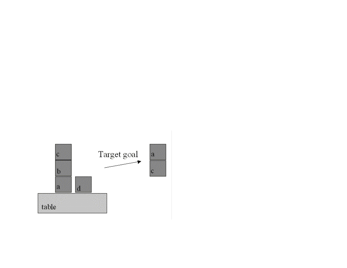
67
The template goal has two slots: a supporting block name and the block sitting on top of this first block):
(deftemplate goal
(slot supporting_block)
(slot supported_block))
As with our previous Jess example, the rule startup is eligible to execute after calling the functions (reset) and (run).
(defrule startup "This is executed when (reset) (run) is executed"
=>
(assert (goal (supporting_block C) (supported_block A)))
(assert (block (name A) (supporting B)))
(assert (block (name B) (on_top_of A) (supporting C)))
(assert (block (name C) (on_top_of B)))
(assert (block (name D)))
(assert (block (name table) (supporting A)))
(assert (block (name table) (supporting C))))
Figure 3.1 shows the initial block setup and the goal state created by the rule startup.
Figure 3.1 The goal set up in the rule startup is to get block a on top of block c
The following rule set-block-on attempts to move one block on top of another. There are two preconditions for this rule to fire:
Both blocks must not have any other blocks on top of them

68
We can not already have cleared the bottom block (this condition is prevent infinite loops)
We see a condition on the matching process in the second LHS element: the matching variable ?block_2 can not equal the matching
variable ?block_1. Here, we use the not-equals function neq; the corresponding equals function is eq.
(defrule set-block-on "move ?block_1 to ?block_2 if both
are clear"
?fact1 <- (block (name ?block_1)
(on_top_of ?on_top_of_1)
(supporting nothing))
?fact2 <- (block (name ?block_2&:(neq ?block_2 ?block_1))
(supporting nothing)
(on_top_of ?on_top_of_2))
?fact3 <- (block (name ?on_top_of_1)
(supporting ?block_1)
(on_top_of ?on_top_of_3))
(not (old_block_state (name ?block_2)
(on_top_of ?on_top_of_2) (supporting ?block_1)))
=>
(retract ?fact1)
(retract ?fact2)
(retract ?fact3)
(assert (block (name ?block_1) (on_top_of ?block_2)
(supporting nothing)))
(assert (block (name ?block_2) (on_top_of ?on_top_of_2)
(supporting ?block_1)))
(assert (old_block_state (name ?block_2)
(supporting nothing) (on_top_of ?on_top_of_2)))
(assert (block (name ?on_top_of_1) (supporting nothing)
(on_top_of ?on_top_of_3)))
(printout t "Moving " ?block_1 " from " ?on_top_of_1
" to " ?block_2 crlf))
The following rule clear-block has two pre-conditions:
That the block being removed from another block has nothing on top of it
That the block being moved is not already on the table
(defrule clear-block "remove ?block_1 from ?block_2 if ?block1 is
clear"
?fact1 <- (block (name ?block_1)
(on_top_of ?block_2&:(neq ?block_2 table))
(supporting nothing))
?fact2 <- (block (name ?block_2) (supporting ?block_1)
(on_top_of ?on_top_of_2))
=>

69
(retract ?fact1)
(retract ?fact2)
(assert (block (name ?block_1)
(on_top_of table)
(supporting nothing)))
(assert (block (name ?block_2) (on_top_of ?on_top_of_2)
(supporting nothing)))
(assert (block (name table) (supporting ?block_1)))
(printout t "Clearing " ?block_1 " from " ?block_2
" on to table" crlf))
The following rule my-halt-rule has a new feature: changing a rule’s default execution priority (or salience). The default rule salience
is zero, but by setting the salience for my-halt-rule to a high value, we are guaranteed that this rule will immediately execute as soon
as its conditions are met:
(defrule my-halt-rule "to stop when the goal is reached"
(declare (salience 100))
(goal (supporting_block ?b1) (supported_block ?b2))
(block (name ?b1) (supporting ?b2))
=>
(printout t "Done: goal is satisfied" crlf)
(halt))
The RHS action function (halt) immediately stops the Jess interpreter.
Note that on any execution cycle, more than one rule may be eligible to execute because all of its preconditions are satisfied. Choosing
which rule to execute is called conflict resolution. The conflict set is the set of rules that are currently eligible to execute. The default
conflict resolution strategy implements what is effectively a depth first search strategy because rules are assigned a higher priority if
the working memory elements (i.e., facts) that satisfy their preconditions (i.e., LHS terms) are newer (i.e., have been more recently
added to working memory). The following statement in the reasoning.clp input file changes the default strategy to a breadth first
search:
(set-strategy breadth)
The following four function calls at the bottom of the reasoning.clp input file reset the system, run the Jess interpreter for 20 cycles
(or until the halt function is executed), and then prints out the facts left in the system after the interpreter has halted:
(reset)
(run 20)
(printout t crlf "Facts in system at the end of the run:" crlf)
(facts)
The following listing shows the output generated from loading the reasoning.clp input file into the Jess system:

70
C:\Jess51> java jess.Main reasoning.clp
Jess, the Java Expert System Shell
Copyright (C) 1998 E.J. Friedman Hill and the Sandia Corporation
Jess Version 5.1 4/24/2000
Clearing C from B on to table
Clearing B from A on to table
Moving C from table to D
Clearing C from D on to table
Moving A from table to B
Clearing A from B on to table
Moving C from table to table
Moving B from table to D
Clearing B from D on to table
Moving A from table to C
Done: goal is satisfied
Facts in system at the end of the run:
f-0 (initial-fact)
f-1 (goal (supporting_block C) (supported_block A))
f-15 (old_block_state (name D) (on_top_of table) (supporting nothing))
f-22 (old_block_state (name B) (on_top_of table) (supporting nothing))
f-27 (block (name table) (on_top_of table) (supporting C))
f-28 (old_block_state (name table) (on_top_of table) (supporting nothing))
f-29 (block (name table) (on_top_of table) (supporting nothing))
f-32 (block (name B) (on_top_of table) (supporting nothing))
f-33 (block (name D) (on_top_of table) (supporting nothing))
f-34 (block (name table) (on_top_of table) (supporting B))
f-35 (block (name A) (on_top_of C) (supporting nothing))
f-36 (block (name C) (on_top_of table) (supporting A))
f-37 (old_block_state (name C) (on_top_of table) (supporting nothing))
For a total of 13 facts.
If you try writing your own rules, you will probably be surprised that at least initially, the rules to not do what you expected! There are
a few techniques that will help you get started. Pay attention to Jess error messages! You will probably see both compiler errors and
runtime errors. Compiler errors indicate the line number in the input file where the error occurred and frequently a hint; for example:
“missing )”. Runtime errors will usually indicate which rule was executing when the error occurred. Another technique for getting
your rules to execute properly is to set up small test cases, and print the contents of working memory using the function (facts) before
and after running the system. Another good technique is to call the function (run 1) with an argument of one to only run one cycle at a
time; you can then examine working memory by calling the (facts) function.
3.3 Embedding Jess Expert Systems in Java Programs

71
We will use the cooking rule set from Section 3.1 to create a simple example Java program that uses the Jess system. First, we modify
the food.clp file, changing the name to food_rules.clp, removing the initial facts definitions and the (reset) and (run) commands:
;; File: food_rules.clp
;;
;; A simple example to introdue CLIPS/Jess programming
(defrule thaw-frozen-food ""
?fact <- (have_food (name ?name) (is_frozen yes) (weight ?w))
=>
(retract ?fact)
(assert (have_food (name ?name) (weight ?w) (is_frozen no)))
(printout t "Using the microwave to thaw out " ?name crlf)
(printout t "Thawing out " ?name " to produce "
?w " ounces of " ?name crlf)
(assert (cooked-food ?name used-microwave)))
When embedding Jess expert systems in your Java programs, you will probably want to use the following strategy:
1. Create an instance of the Rete class
2. Create an instance of the Jesp class and use it to read a file containing Jess rules into the memory managed my the Rete class
instance
3. Add working memory elements for the problem that you want to solve
4. Run the Rete class instance to interpret rules
5. Examine working memory – your rules should have placed new working memory element(s) that your Java program can detect
and use
When you download CLIPS version 6, you will notice the documentation directory. This contains JavaDoc style documentation for the
Jess Java classes. The Jess class that we need to use when embedding Jess is the Rete class. We will look at a simple Java program that
uses the Rete class, then discuss the code:
import java.util.*;
import java.io.*;
import jess.*;
public class Food {
public static void main(String[] args) {
try {
FileReader fr = new FileReader("food_rules.clp");
Rete r = new Rete();
Jesp jesp = new Jesp(fr, r);

72
jesp.parse(false);
r.executeCommand("(reset)");
r.executeCommand(
"(assert (have_food (name spinach) (weight 10)))");
r.executeCommand(
"(assert (have_food (name peas) (weight 14) (is_frozen yes)))");
System.out.println(
"Output from executing up to 10 Jess rules:\n");
// Note: the following command causes any 'printout' commands
// from Jess to print to standard output:
r.executeCommand("(run 10)"); // run a maximum of 10 rule firings
// print out all facts in the system:
System.out.println(
"\nList of all facts asserted in the system:\n");
Iterator iter = r.listFacts();
while (iter.hasNext()) {
System.out.println("Current fact: " + iter.next());
}
} catch (Exception ex) {
System.err.println(ex);
}
}
}
This example prints any rule output to standard output which is not particularly useful for an embedded application. After the rule(s)
have fired, this program uses the listFacts Rete class method to get a Java Iterator for all working memory elements. In a real
embedded application, you would examine working memory to extract results. Here is the output from running this example program:
Output from executing up to 10 Jess rules:
Using the microwave to thaw out peas
Thawing out peas to produce 14 ounces of peas
List of all facts asserted in the system:
Current fact: (MAIN::initial-fact)
Current fact: (MAIN::have_food (name spinach) (weight 10) (is_frozen no))
Current fact: (MAIN::have_food (name peas) (weight 14) (is_frozen no))
Current fact: (MAIN::cooked-food peas used-microwave)
The last fact in working memory was added when the rule thaw_frozen_food executed.
The Rete class also has a mechanism for specifying callback for Jess events like rule firings and working memory changes. This is a
more complex, but probably good technique for complex embedded expert system applicastions.

73
This Java program is simple, but does demonstrate the basic steps that you need to take to embed an expert system in a Java program.
You should write and debug your rules using Jess interactively as we did in Sections 3.1 and 3.2. After your expert system works then
you can embed it.

74
Chapter 4. Genetic Algorithms
We will see how AI systems can be evolved using genetic algorithms (GA) in this chapter. There are two schools of thought on
building AI systems: encoding knowledge “by hand” using a knowledge representation language like we did in Chapter 3 or allowing
a system to evolve internal state and behavior while interacting with its environment. The AI programming techniques of GA is very
useful for AI systems that must adapt to changing conditions. You will probably find GAs to be more practical for your AI
programming projects. The examples for this chapter are in the directory:
src
src/ga – genetic algorithm code
GAs are typically used to search very large and possibly very high dimensional search spaces. Using a GA toolkit, like the one
developed in Section 4.1, requires two problem-specific customizations:
Characterize the search space by a set of parameters that can be encoded in a chromosome (more on this later). GAs work with the
coding of a parameter set, not the parameters themselves (Goldberg, 1989).
Provide a numeric fitness function that allows us to rate the fitness of each chromosome in a population. We will use these fitness
values to determine which chromosomes in the population are most likely to survive and reproduce using genetic crossover and
mutation operations.
The GA toolkit developed in this Chapter treats genes as a single bit; while you can consider a gene to be an arbitrary data structure,
the approach of using single bit genes and specifying the number of genes (or bits) in a chromosome is very flexible. A population is
a set of chromosomes. A generation is defined as one reproductive cycle of replacing some elements of the chromosome population
with new chromosomes produced by using a genetic crossover operation followed by optionally mutating a few chromosomes in the
population.
We will start the introduction to GAs by walking through a very simple example, then discuss some of the advantages of using GAs
before implementing the toolkit in Section 4.1. In Section 6.2, we will use this GA toolkit to solve a regression problem. For the
remainder of this session, we will solve this first example problem by writing the customizations for the GA toolkit that we will
discuss in detail in Section 4.1.
For a sample problem, suppose that we want to find the maximum value of the function F with one independent variable x:
F(x) = sin(x) * sin(0.4 * x) * sin(3 * x)
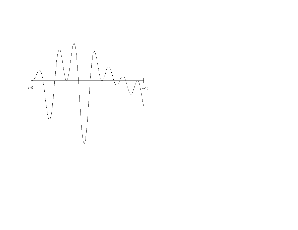
75
over the interval [0, 10]. This function is plotted in Figure 4.1. The problem that we want to solve is finding a good value of X to find
the largest possible value of F(x).
Figure 4.1 The test function evaluated over the interval [0.0, 10.0]. The maximum value of 0.56 occurs at x=3.8. This plot was
produced by the file src/ga/misc/Graph.java.
While this problem can be solved trivially by a brute force search over the range of the independent variable x, the GA method scales
very well to similar problems of a higher dimensionality; for example, we might have products of sine waves using 20 independent
variables x1, x2, ..x20. In this case, a brute force search would be prohibitively expensive. Still, the one-dimensional case seen in
Figure 4.1 is a good starting point for discussing GAs.
Out first task is to characterize the search space as one or more parameters. In Section 4.2, we will show how to encode several
parameters in a single chromosome, but in this problem, we have only one parameter, the independent variable x. For this example, we
will choose to encode the parameter x using ten bits (so we have ten 1-bit genes per chromosome). A good starting place is to write
utility method for converting the 10-bit representation to a floating-point number in the range [0.0, 10.0]:
float geneToFloat(int geneIndex) {
76
int base = 1;
float x = 0;
for (int j=0; j<numGenes; j++) {
if (getGene(geneIndex, j)) {
x += base;
}
base *= 2;
}
x /= 128.0f; // hard wired for 10-bit chromosomes
return x;
}
Note that we do not need the reverse method! The GA toolkit will create population of 10-bit chromosomes; in order to evaluate the
fitness of each chromosome in a population, we only have to convert the 10-bit representation to a floating-point number for
evaluation using the following fitness function:
float fitness(float x) {
return (float)(Math.sin(x) * Math.sin(0.4f * x) *
Math.sin(3.0f * x));
}
That is all there is to it! Problem solved! Table 4.1 shows the results of a run, using the GA toolkit in src/ga. As seen in Table 4.1, for
this “easy problem”, the GA quickly settles on a good answer, very close to the function’s maximum value in the interval 0.0, 10.0].
Table 4.1
Generation number
X for best fitness
Best fitness value
Average fitness value
0
2.67
0.391
-0.038
1
2.67
0.391
0.352
2
2.64
0.417
0.392
7
2.64
0.417
0.416
8
3.64
0.474
0.419
16
3.64
0.474
0.472
20
3.70
0.526
0.470
21
3.73
0.545
0.515
Now that we have seen how easy it is to run GA experiments like solving the problem in Figure 4.1, we will “go behind the scenes” to
see how GAs work. After this discussion, implementing the toolkit in Section 4.1 will be straightforward. A GA framework provides
the following behavior:
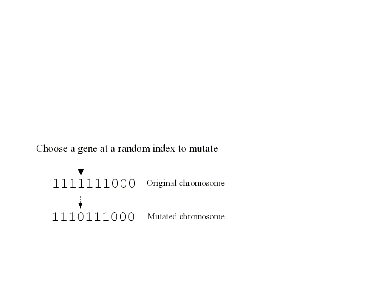
77
Generates an initial random population with a specified number of bits (or genes) per chromosome and a specified number of
chromosomes in the population
Ability to evaluate each chromosome based on a numeric fitness function
Ability to create new chromosomes from the most fit chromosomes in the population using the genetic crossover and mutation
operations
Figure 4.2 shows a sample crossover operation for chromosomes with ten bits per chromosome. Crossover works by choosing two
chromosomes and a random gene (or in our case bit) index where the chromosomes will be split. After splitting each chromosome, the
split parts are switched producing two new chromosomes from the two original chromosomes. Crossover reproduction will be used by
the GA toolkit for creating a new population of chromosomes from an existing population.
Figure 4.2 Crossover operation
Figure 4.3 shows the operation of the genetic mutation operation on a chromosome with ten genes (or bits). A random gene (or bit) is
chosen and its value is reversed.
Figure 4.3 Mutation operation
4.1 Java classes for Genetic Algorithms

78
The classes developed in this section are located in the src/ga directory. The GA toolkit is contained in the Java class Genetic, and the
file TestGenetic.java contains a subclass of Genetic that solves the problem shown in Figure 4.1. The class Genetic is abstract: you
must subclass Genetic and implement the method:
public void calcFitness()
in your derived class; we will see how this is done later in the TestGenetic class. The primary class data that must be stored and
maintained is an array of chromosomes and an associated array of fitness values; it is this array of fitness values that must be set in the
method calcFitness. The Java class BitSet is used to represent a chromosome; this works well because the BitSet class stores sets of
bits efficiently and has a good API for accessing and modifying the elements of the set.
There are two class constructors for Genetic:
public Genetic(int num_genes_per_chromosome,
int num_chromosomes)
public Genetic(int num_genes_per_chromosome,
int num_chromosomes,
float crossover_fraction,
float mutation_fraction)
The optional constructor argument crossover_fraction sets the fraction of chromosomes in the population that considered for the
genetic crossover operation. This value could be in the range [0.0, 1.0], but for practical applications, I usually set it to a value in the
interva [0.1, 0.5]. The optional constructor argument mutation_fraction sets the fraction of chromosomes that undergo mutation each
generation.
The constructors build an array of integers rouletteWheel which is used to weight the most fit chromosomes in the population for
being the parents of crossover operations. When a chromosome is being chosen, a random integer is selected that is used as an index
into the rouletteWheel array; the values in the array are all in the range of [0, number of genes per chromosome – 1]. More fit
chromosomes are heavily weighted in favor of being chosen as parents for the crossover operations. The algorithm for the crossover
operation is fairly simple; here is the implementation:
public void doCrossovers() {
int num = (int)(numChromosomes * crossoverFraction);
for (int i=num-1; i>=0; i--) {
int c1 =
(int)(rouletteWheelSize * Math.random() * 0.9999f);
int c2 =
(int)(rouletteWheelSize * Math.random() * 0.9999f);
c1 = rouletteWheel[c1];
c2 = rouletteWheel[c2];
if (c1 != c2) {
int locus = 1 +

79
(int)((numGenesPerChromosome - 2) * Math.random());
for (int g=0; g<numGenesPerChromosome; g++) {
if (g < locus) {
setGene(i, g, getGene(c1, g));
} else {
setGene(i, g, getGene(c2, g));
}
}
}
}
}
The class variable crossOverFraction is used to calculate the number of chromosomes in the population will be replaced by the
results of crossover reproduction. The array of chromosomes has been sorted in decreasing order of fitness before this method is
called, so the least fit individuals are at the higher array indices; these individuals will be replaced. Two chromosome indices c1 and
c2 are calculated using a random number generator and the rouletteWheel array. The index locus is a random value in the range [1,
number of bits per chromosome – 2]. Remember that all indexing is zero based. Genes at index less than locus are copied from the
beginning of the chromosome indexed by c1 and genes at index greater than or equal to locus are replaced by the genes at the end of
the chromosome indexed by c2.
The algorithm for mutating a chromosome is simple: randomly choose a gene and flip its value.
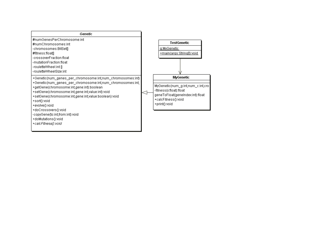
80
Figure 4.4 UML class diagrams for genetic algorithm Java classes
The method sort re-orders both the chromosome array and the associated fitness array in decreasing order of fitness. The top level
control method in class Genetic is evolve. This method is called once per generation and performs the following actions:
Calculates the fitness of the chromosomes in the population by calling the abstract method calcFitness
Sort the chromosomes in decreasing order of fitness by calling method sort
Perform genetic crossover reproductions by calling method doCrossOvers
Perform genetic mutations by calling method doMutations
We will now return to the simple problem seen in Figure 4.1. We need to write two classes, which I call:
MyGenetic – a subclass of Genetic that provides a utility method to convert a gene to a floating point value and defines the method
calcFitness
TestGenetic – a main program that creates an instance of class MyGenetic and calls the evolve and print methods for this instance
of MyGenetic in a loop over generations

81
Note that the class MyGenetic is defined as an inner class in the file TestGenetic.java. The only interesting methods that we need to
define are MyGenetic.calcFitness and the utility method that it calls MyGenetic.geneToFloat. We already saw the implementation of
these methods in the introduction to this chapter.
4.2 Example System for solving polynomial regression problems
We will look at a more interesting problem in this section: solving a polynomial regression problem. We will try to fit the following
function in both this section and in Chapter 7 using genetic programming techniques:
F(X) = X*X*X*X + X*X*X + X*X + X
We will attempt to fit the following fourth degree polynomial function with 5 constant coefficients A,B,C,D,E by searching for good
vales for A,B,C,D, and E:
F(X) = A*X*X*X*X + B*X*X*X + C*X*X + D*X + E
Clearly, we want:
A = B = C = D = 1.0
E = 0.0
In this problem, the chromosomes must encode the values of the 5 constant coefficients. We implement this example using the classes
(source files are in the directory src/ga):
RegressionTest – contains a main program that creates an instance of the class RegressionGenetic and runs several generations
RegressionGenetic – derived from the class Genetic
The class RegressionGenetic is defined as a utility class in the file RegressionTest.java. The method
RegressionGenetic.geneToFloat is used to extract any of the five coefficients from a specified chromosome:
float geneToFloat(int chromosomeIndex, int numberIndex) {
int base = 1;
float x = 0;
for (int j=0; j<bitsPerNumber; j++) {
if (getGene(chromosomeIndex,
j + numberIndex * bitsPerNumber))
{

82
x += base;
}
base *= 2;
}
x /= normalization;
x -= 5.0f;
if (gmin > x) gmin = x;
if (gmax < x) gmax = x;
return x;
}
The class RegressionGenetic supports any number of bits (or genes) per coefficient; the class constructor terminates with an error if
the specified number of bits (or genes) per chromosome is not evenly divisible by 5. The fitness function calcFitness evaluates each
chromosome by extracting the 5 coefficient values for each chromosome and then calling the auxiliary method
calcFitnessForCoefficients:
public void calcFitness() {
for (int i=0; i<numChromosomes; i++) {
for (int j=0; j<5; j++) {
coefficients[j] = geneToFloat(i, j);
}
fitness[i] = calcFitnessForCoefficients(coefficients);
}
}
The definition of calcFitnessForCoefficients is:
private float calcFitnessForCoefficients(float [] coef) {
float ret = 0.0f;
// evaluate function error over a range of values of x:
for (float x=0.0f; x<=10.0f; x+= 0.05) {
// true value of regression function:
float Ftrue = x*x*x*x + x*x*x + x*x + x;
// value of generated function at x:
float F = coef[0] * x*x*x*x +
coef[1] * x*x*x +
coef[2] * x*x +
coef[3] * x +
coef[4];
ret += (F - Ftrue) * (F - Ftrue);
}
return 25000.0f - ret;
}
83
Note that the scaling (and any offsets) of fitness values is immaterial as long as the ranking preserves the order best chromosomes
having higher fitness values; the constant 25000.0f in this method was merely chosen to place fitness values in a reasonable numeric
range for viewing.
Table 4.2 shows the results of an example run where we allow just four bits per encoded coefficient. At this “coarse resolution”,
allowed values for the independent variable are (-5, -4.5, -4, -3.4, -3, -2.5, -2, -1.5, -1, -0.5, 0, 0.5, 1, 1.5, 2, 2.5), sixteen possible
values in all. The constructor call for this experiment uses 20 genes per chromosome (4 bits per coefficient), a population size of 300,
a 0.98 crossover fraction, and 0.05 mutation rate; here is the constructor call:
g = new RegressionGenetic(20, 300, 0.98f, 0.05f);
Table 4.2 – Best of generation evolved coefficients (best fit is all equal to 1.0, except E=0)
Generation
A
B
C
D
E
1
1.5
1.5
2.0
-1.5
-0.5
2
1.0
0.5
2.5
2.5
-3.0
3
1.0
1.0
2.0
-4.5
-2.0
4
1.0
1.0
1.0
-1.5
-0.5
6
1.0
1.0
1.0
1.0
1.5
8
1.0
1.0
1.0
1.0
0.0
Even though this problem is of moderate dimensionality (with 5 dimensions), the coarseness of the number representations combined
with the “lucky accident” of the existence of the two necessary coefficient values of 0.0 and 1.0, makes this a fairly uninteresting
experiment. We have already found a perfect chromosome in the population by generation 7 using a fairly small population of just 300
chromosomes; there is a tradeoff in population size versus the number of generation necessary to find a fit individual (i.e., a
chromosome that encodes a solution to the problem that we are trying to solve).
In Table 4.3, instead of just using 4 bits to encode each coefficient, we will use 6 bits (so we get 64 possible values instead of 16). This
is a fair test of the GA toolkit. For this evolutionary experiment, we use a much larger population (5000 chromosomes), and find a
perfect chromosome in the population by generation 5:
Table 4.3 Best of generation evolved coefficients (best fit is all equal to 1.0, except E=0)
Generation
A
B
C
D
E
84
1
-0.875
2.2125
-0.75
-5.0
-2.125
2
1.0
2.0
1.25
-3.875
-3.875
3
1.0
1.0
1.125
0.125
-3.125
4
1.0
1.0
1.125
0.125
-0.875
5
1.0
1.0
1.0
1.
0.0
This second example shows that as the complexity of the data that is represented in a chromosome increases, that it is efficient to
greatly increase the population size in order to find a fit individual in a small number of generations.

85
Chapter 5. Neural networks
I believe that the techniques for using neural networks efficiently solve many problems that are intractable or difficult using other AI
programming techniques. Although most of this book is intended to provide practical advice (with some theoretical background) on
using AI programming techniques, I can not imagine being interested in practical AI programming without also wanting to think about
the philosophy and mechanics of how the human mind works. I hope that my readers share this interest and later I will discuss “real
neurons”, etc.
The examples for this chapter are in the directory:
src
src/neural – Hopfield and Back Propagation neural network code
In this book, we have examined techniques for focused problem solving, concentrating on performing one task at a time. However, the
physical structure and dynamics of the human brain is inherently parallel and distributed [Rumelhart, McClelland, etc. 1986]. We are
experts at doing many things at once. For example, I simultaneously can walk, talk with my wife, keep our puppy out of cactus, and
enjoy the scenery behind our house in Sedona Arizona. AI software systems struggle to perform even narrowly defined tasks well, so
how is it that we are able to simultaneously perform several complex tasks? There is no clear and absolute answer to this question at
this time, but certainly the distributed neural architecture of our brains is a requirement for our abilities.
Also interesting is the distinction between instinctual behavior and learned behavior. Our knowledge of GAs from Chapters 4 provides
a clue to how the brains of especially lower order animals can be hardwired to provide efficient instinctual behavior under the
pressures of evolutionary forces (i.e., likely survival of more fit individuals). While we will study supervised learning techniques in
this chapter, it is possible to evolve both structure and attributes of neural networks using GA techniques [Watson, 1995], and some
neural network models like ART autonomously learn to classify learning examples without intervention.
We will start this chapter by discussing human neuron cells and what features of real neurons that we will model. Unfortunately, we do
not yet understand all of the biochemical processes that occur in neurons, but there are fairly accurate models available (web search
“neuron biochemical”). Neurons are surrounded by thin hair like structures called dendrites, which serve to accept activation from
other neurons. Neurons sum up activation from their dendrites and each neuron has a threshold value; if the activation summed over
all incoming dendrites exceeds this threshold, then the neuron fires, spreading its activation to other neurons. Dendrites are very
localized round a neuron. Output from a neuron is carried by an axon, which is thicker than dendrites and potentially much longer than
dendrites in order to affect remote neurons. Figure 5.1 shows the physical structure of a neuron; in general, the neuron’s axon would
be much longer than is seen in Figure 5.1. The axon terminal buttons transfer activation to the dendrites of neurons that are close to the
individual button. An individual neuron is connected to up to ten thousand other neurons in this way.
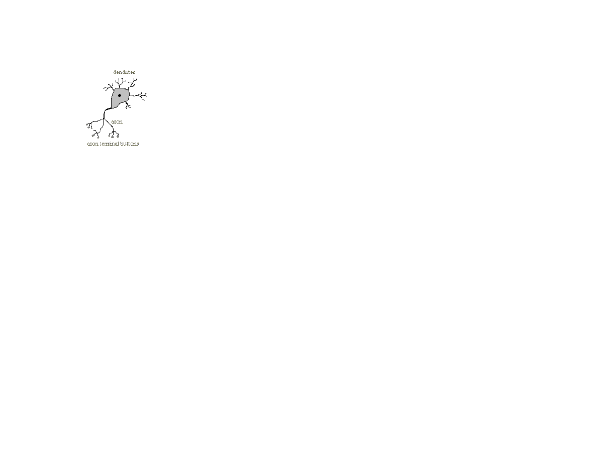
86
Figure 5.1 Physical structure of a neuron
The activation absorbed through dendrites is summed together, but the firing of a neuron only occurs when a threshold is passed.
5.1 Hopfield neural networks
Hopfield neural networks implement associative (or content addressable) memory. A Hopfield network is trained using a set of
patterns. After training, the network can be shown a pattern similar to one of the training inputs and it will hopefully associate the
“noisy” pattern with the correct input pattern. Hopfield networks are very different that back propagation networks because the
training data only contains input examples. Internally, the operation of Hopfield neural networks is very different that back
propagation networks that we will see later in this chapter. We use Hopfield neural networks to introduce the subject of neural nets
because they are very easy to simulate with a program, and they can also be very useful in practical applications.
The inputs to Hopfield networks can be any dimensionality. Often, Hopfield networks are shown as having a two-dimensional input
field and are demonstrated recognizing characters, pictures of faces, etc. However, we will loose no generality by implementing a
Hopfield neural network toolkit with one-dimensional inputs because a two-dimensional image can be “liberalized” into an equivalent
one-dimensional array.
How do Hopfield networks work? A simple analogy will help. The trained connection weights in a neural network represent a high
dimensional space. This space is folded and convoluted with local minima representing areas around training input patterns. For a
moment, visualize this very high dimensional space as just being the three dimensional space inside a room. Now, the floor of this
room is a convoluted and curved surface. If you pick up a basketball and bounce it around the room, it will settle at a low point in this
curved and convoluted floor. Now, consider that the space of input values is a two dimensional grid a foot above the floor. For any
new input, that is equivalent to a point defined in horizontal coordinates; if we drop our basketball from a position above an input grid
point, the basketball will tend to roll down hill into local gravitational minima. Now, the shape of the curved and convoluted floor is a

87
calculated function of a set of training input vectors. After the “floor has been trained” with a set of input vectors, then the operation of
dropping the basketball from an input grid point is equivalent to mapping a new input into the training example that is closest to this
new input using a neural network.
A common technique in training and using neural networks is to add noise to training data and weights. In the basketball analogy, this
is equivalent to “shaking the room” so that the basketball finds a good minima to settle into, and not a non-optimal local minima. We
use this technique later when implementing back propagation networks. The weights of back propagation networks are also best
visualized as defining a very high dimensional space with a manifold that is very convoluted with areas of local minima defined
centered near coordinates defined by an input vector.
5.2 Java classes for Hopfield neural networks
The Hopfield neural network model is defined in the file src/neural/Hopfield.java. Since this file only contains about 65 lines of
code, we can review both the code and the algorithms for storing and recall of patterns at the same time. In a Hopfield neural network
simulation, every neuron is connected to every other neuron.
Consider a pair of neurons indexed by i and j. We can define energy between the associations of these two neurons as:
energy[i,j] = - weight[i,j] * activation[i] * activation[j]
In the Hopfield neural network simulator, we store activations (i.e., the input values) as floating point numbers that get clamped in
value to –1 (for off) or +1 (for on). In the energy equation, we consider an activation that is not clamped to a value of one to be zero.
This energy is analogous to “gravitational energy potential” in the basketball analogy. For a new input, we are looking for a low
energy point near the new input vector. The total energy is a sum of the above equation over all (i,j).
The class constructor allocates storage for input values, temporary storage, and a two dimensional array to store weights:
public Hopfield(int numInputs) {
this.numInputs = numInputs;
weights = new float[numInputs][numInputs];
inputCells = new float[numInputs];
tempStorage = new float[numInputs];
}
Remember that this model is general purpose: multi-dimensional inputs can be converted to an equivalent one-dimensional array. The
method addTrainingData is used to store another input data array for later training. All input values get clamped to an “off” or “on”

88
value by the utility method adjustInput. The utility method truncate truncates floating-point values to an integer value. The utility
method deltaEnergy has one argument: the index of the input vector. The class variable tempStorage is set during training to be the
sum of a row of trained weights. So, the method deltaEnergy returns a measure of the energy difference between the input vector in
the current input cells and the training input examples:
private float deltaEnergy(int index) {
float temp = 0.0f;
for (int j=0; j<numInputs; j++) {
temp += weights[index][j] * inputCells[j];
}
return 2.0f * temp - tempStorage[index];
}
The method train is used to set the two dimensional weight array and the one dimensional tempStorage array in which each element
is the sum of the corresponding row in the two dimensional weight array:
public void train() {
for (int j=1; j<numInputs; j++) {
for (int i=0; i<j; i++) {
for (int n=0; n<trainingData.size(); n++) {
float [] data = (float [])trainingData.elementAt(n);
float temp1 =
adjustInput(data[i]) * adjustInput(data[j]);
float temp = truncate(temp1 + weights[j][i]);
weights[i][j] = weights[j][i] = temp;
}
}
}
for (int i=0; i<numInputs; i++) {
tempStorage[i] = 0.0f;
for (int j=0; j<i; j++) {
tempStorage[i] += weights[i][j];
}
}
}
Once the arrays weight and tempStorage are defined, it is simple to recall an original input pattern from a similar test pattern:
public float [] recall(float [] pattern, int numIterations) {
for (int i=0; i<numInputs; i++) inputCells[i] = pattern[i];
for (int ii = 0; ii<numIterations; ii++) {
for (int i=0; i<numInputs; i++) {
if (deltaEnergy(i) > 0.0f) {
inputCells[i] = 1.0f;
} else {
inputCells[i] = 0.0f;
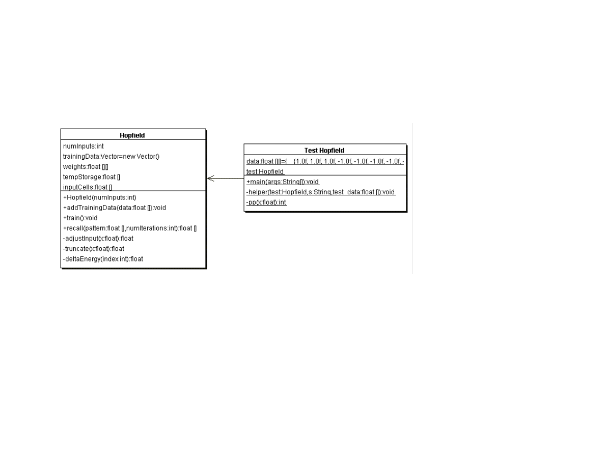
89
}
}
}
return inputCells;
}
Figure 5.2 shows the UML class diagram for both the Hopfield class and a text based test program.
Figure 5.2 UML class diagram for the Hopfield class and the test class Test_Hopfield
5.3 Testing the Hopfield neural network example class
The test program for the Hopfield neural network class is Test_Hopfield. This test program defined three test input patterns, each with
ten values:
static float [] data [] = {
{ 1, 1, 1, -1, -1, -1, -1, -1, -1, -1},
{-1, -1, -1, 1, 1, 1, -1, -1, -1, -1},
{-1, -1, -1, -1, -1, -1, -1, 1, 1, 1}
};
The following code fragment shows how to create a new instance of the Hopfield class and train it to recognize these three test input
patterns:

90
test = new Hopfield(10);
test.addTrainingData(data[0]);
test.addTrainingData(data[1]);
test.addTrainingData(data[2]);
test.train();
The static helper method is used to slightly scramble an input pattern, then test the training Hopfield neural network to see if the
original pattern is re-created:
helper(test, "pattern 0", data[0]);
helper(test, "pattern 1", data[1]);
helper(test, "pattern 2", data[2]);
Here is the implementation of the helper method (the called method pp simply formats a floating point number for printing by
clamping it to zero or one):
private static void helper(Hopfield test, String s,
float [] test_data) {
float [] dd = new float[10];
for (int i=0; i<10; i++) {
dd[i] = test_data[i];
}
int index = (int)(9.0f * (float)Math.random());
if (dd[index] < 0.0f) dd[index] = 1.0f;
else dd[index] = -1.0f;
float [] rr = test.recall(dd, 5);
System.out.println(s);
for (int i=0; i<10; i++) System.out.print(pp(rr[i]) + " ");
System.out.println();
}
Listing 5.1 shows how to run the program, and lists the example output.
Listing 5.1
java Test_Hopfield
pattern 0
1 1 1 0 0 0 0 0 0 0
pattern 1
0 0 0 1 1 1 0 0 0 0
pattern 2
0 0 0 0 0 0 0 1 1 1
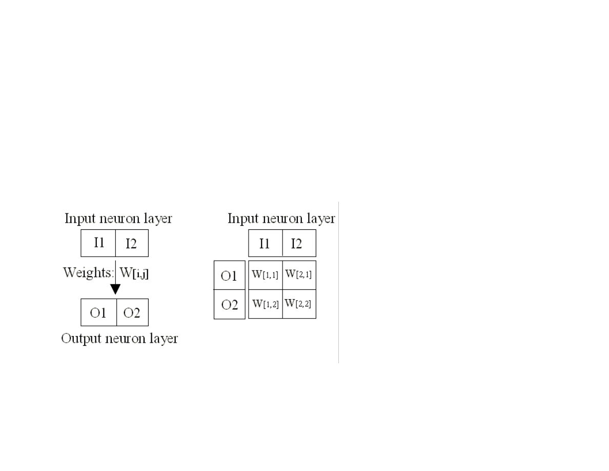
91
In Listing 5.1, we see that the three sample training patterns defined in Test_Hopfield.java are re-created after scrambling the data by
changing one randomly chosen value to its opposite value.
5.5 Backpropagation neural networks
The next neural network model that we will use is called back propagation, also known as back-prop and delta rule learning. In this
model, neurons are organized into data structures that we call layers. Figure 5.3 shows a simple neural network with two layers; this
network is shown in two different views: just the neurons organized as two one-dimensional arrays, and as two one-dimensional arrays
with the connections between the neurons. In our model, there is a connection between two neurons that is characterized by a single
floating-point number that we will call the connection’s weight. A weight W[i,j] connects input neuron i to output neuron j. In the
back propagation model, we always assume that a neuron is connected to every neuron in the previous layer. In Figure 5.3, we only
have two neuron layers, one for the input neurons and one for the output neurons.
Figure 5.3 Two views of a two layer neural network; the view on the right also shows the connection weights between the input
and output layers.
To calculate the activation of the first output neuron O1, we evaluate the sum of the products of the input neurons times the
appropriate weight values; this sum is input to a Sigmoid activation function (see Figure 5.4) and the result is the new activation value
for O1. Here is the formula for the simple network in Figure 5.3:
O1 = Sigmoid (I1 * W[1,1] + I2 * W[2,1])
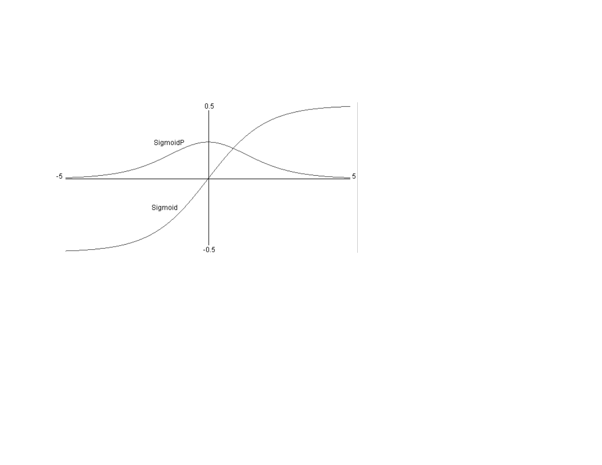
92
O2 = Sigmoid (I2 * W[1,2] + I2 * W[2,2])
Figure 5.4 shows a plot of the Sigmoid function and the derivative of the sigmoid function (SigmoidP). We will use the derivative of
the Sigmoid function when training a neural networks (with at least one hidden neuron layer) with classified data examples.
Figure 5.4 Sigmoid and derivative of the Sigmoid (SigmoidP) functions. This plot was produced by the file
src/neural/misc/Graph.java. NOTE (3/11/2004): I changed the range of the Sigmoid function to [0, 1] instead of [-0.5, +0.5] –
either range works well, but most Sigmoid functions in published literature seem to use the range [0, 1], so I changed the range
I use to avoid confusion.
A neural network like the one seen in Figure 5.3 is trained by using a set of training data. For back propagation networks, training
data consists of matched sets of input and output values. We want to train a network to not only produce the same outputs for training
data inputs as appear in the training data, but also to generalize its pattern matching ability based on the training data. A key here is to
balance the size of the network against how much information it must hold. A common mistake when using back propagation
networks is to use too large of a network (more on what this means later); a network that contains too many neurons will simply
memorize the training examples, including any noise in the training data. However, if we use a smaller number of neurons, with a very
large number of training data examples, then we force the network to generalize, ignoring noise in the training data.
How do we train a back propagation neural network given that we have a good training data set? The algorithm is quite easy; we will
now walk through the simple case of a two layer network like the one in Figure 5.3, and later in Section 5.6 we will review the
algorithm in more detail when we have either one or two hidden neuron layers between the input and output layers.
In order to train the network in Figure 5.3, we repeat the following learning cycle several times:
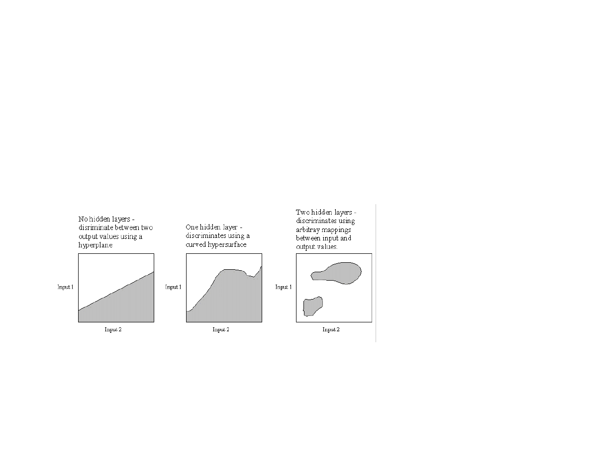
93
Zero out temporary arrays for holding the error at each neuron. The error, starting at the output layer, is the difference between the
output value for a specific output layer neuron and the calculated value from setting the input layer neuron’s activation values to
the input values in the current training example, and letting activation spread through the network.
Update the weight W[i,j] (where i is the index of an input neuron, and j is the index of an output neuron) using the formula W[i,j]
+= learning_rate * output_error[j]*I[i], where the learning_rate is a tunable parameter, output_error[j] was calculated in step
1, and I[i] is the activation of input neuron at index i.
This process is continued to either a maximum number of learning cycles or until the calculated output errors get very small. We will
see later that the algorithm is similar, but slightly more complicated, when we have hidden neuron layers; the difference is that we will
“back propagate” output errors to the hidden layers in order to estimate errors for hidden neurons; more on this later. The type of
neural network is two simple to solve very many interesting problems, and in practical applications we almost always use either one
additional hidden neuron layers or two additional hidden neuron layers. Figure 5.5 shows the types of problems that can be solved by
zero hidden layer, one hidden layer, and two hidden layer networks.
Figure 5.5 Capabilities of zero, one, and two hidden neuron layer neural networks. The grayed areas depict one of two possible
output values based on two input neuron activation values. Note that this is a two dimensional case for visualization purposes;
if a network had ten input neurons instead of two, then these plots would have to be ten dimensional instead of two
dimensional.
5.6 A Java class library and examples for using back propagation neural networks

94
The back propagation neural network library used in this chapter was written to be easily understood and is useful for many problems.
However, one thing that is not in this implementation is something usually called “momentum”: remember how much each weight was
changed in the previous learning cycle and make the weight change larger if the current change in “direction” is the same as the last
learning cycle. For example, if the change to weight Wij had a large positive value in the last learning cycle and the calculated weight
change for Wij is also a large positive value in the current learning cycle, then make the current weight change even larger. Adding a
“momentum” term not only makes learning faster but also increases the chances of sucessfully learning more difficult problems like
XOR. Later in this chapter, I will discuss how to solve XOR using the library (without momentum).
The source directory src/neural contains example programs for both back propagation neural networks and Hopfield neural networks,
which we saw at the beginning of this chapter. The relevant files for the back propagation examples are:
Neural_1H.java – contains a class for simulating a neural network with one hidden neuron layer
Test_1H.java – a text based test program for the class Neural_1H
GUITest_1H.java – a GUI based test program for the class Neural_1H
Neural_2H.java – contains a class for simulating a neural network with two hidden neuron layers
Test_2H.java – a text based test program for the class Neural_2H
GUITest_2H.java – a GUI based test program for the class Neural_2H
Plot1DPanel – a Java JFC graphics panel for the values of a one dimensional array of floating point values
Plot2DPanel – a Java JFC graphics panel for the values of a two dimensional array of floating point values
The four GUI files are for demonstration purposes only, and we will not discuss the code for these classes; if you are interested in the
demo graphics code and do not know JFC Java programming, there are a few good JFC tutorials at the web site java.sun.com. Figure
5.6 shows the UML class diagrams for all of the back propagation classes and the text based test programs, but we will only discuss in
depth the classes Neural_1H and Neural_2H in this text, while quickly reviewing the code in the text based test programs as
examples for setting up neural network problems.
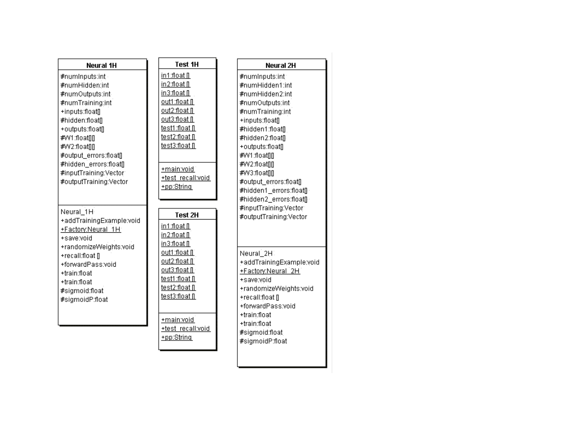
95
Figure 5.6 UML class diagrams for the neural network examples for one hidden layer (classes ending in _1H) and two hidden
layers (classes ending in _2H)
The class Neural_1H contains the following methods:

96
Neural_1H – class constructor requires three arguments: the number of neurons in the input, hidden, an output layers. Storage is
allocated for neuron activations, neuron errors for the hidden and output layers, and weights. The method randomizeWeights is
called to initialize the weight values to random floating point values in the range [-0.05, 0.05].
AddTrainingExample – adds a single training exemplar to the current training data set
Factory – a static function that creates an instance of the Neural_1H class from a serialized file. This method is useful for quickly
loading a neural network that has already been trained into an application program.
save – saves the neural network to a serialized data file that can be efficiently reloaded using the static Factory method
randomizeWeights – sets the weights to random values in the range [-0.5, 0.5]
recall – accepts an array of floating point values that are used to set the activation values of the input layer neurons. The utility
method forwardPass is used to propagate activation values through the network using the current weight values; this results in a
new activation pattern on the output layer neurons.
forwardPass – a utility method that is used to propagate activation values from the input neurons, to the hidden layer neurons, and
finally to the output layer neurons
train – two methods for training one cycle. A cycle is defined as showing the network the training examples one time, and
adjusting the weights in the network based on errors at each neuron.
sigmoid – the Sigmoid function seen in Figure 5.4
sigmoidP – the derivative of the Sigmoid function seen in Figure 5.4
The code in the class Neural_1H is all fairly simple; we will look in detail at only the methods forwardPass and train. The following
code fragment are from the definition of forwardPass.
This code uses the input to hidden layer weights to calculate the activation values of the hidden layer neurons:
for (h=0; h<numHidden; h++) {
hidden[h] = 0.0f;
}
for (i=0; i<numInputs; i++) {
for (h=0; h<numHidden; h++) {
hidden[h] +=
inputs[i] * W1[i][h];
}
}
Similar code calculates the output layer neuron’s activation values:
for (o=0; o<numOutputs; o++)
outputs[o] = 0.0f;
for (h=0; h<numHidden; h++) {
for (o=0; o<numOutputs; o++) {

97
outputs[o] +=
sigmoid(hidden[h]) * W2[h][o];
}
}
for (o=0; o<numOutputs; o++)
outputs[o] = sigmoid(outputs[o]);
Here, we apply the Sigmoid function (seen in Figure 5.4) to the output activation values.
The method train(Vector v_ins, Vector v_outs) is used to make one training cycle. The first thing to be done is to zero out the error
array for the hidden and output layers:
for (h=0; h<numHidden; h++)
hidden_errors[h] = 0.0f;
for (o=0; o<numOutputs; o++)
output_errors[o] = 0.0f;
Next, we copy the input and output values to local arrays for faster data access:
for (i=0; i<numInputs; i++) {
inputs[i] =
((float [])v_ins.elementAt(current_example))[i];
}
float [] outs =
(float [])v_outs.elementAt(current_example);
We use the utility method forwardPass to spread the new input activtions through the neural network:
forwardPass();
Then we calculate adjusted output errors by comparing the output neuron’s spreading activation with the values in this training data
example:
for (o=0; o<numOutputs; o++) {
output_errors[o] =
(outs[o] - outputs[o]) * sigmoidP(outputs[o]);
}
It is a little complicated to approximate the hidden layer neurons we need to backwards propagate the output neuron’s errors, scaling
this by the relative connection weights between the hidden layer and output layer neurons:
for (h=0; h<numHidden; h++) {
hidden_errors[h] = 0.0f;

98
for (o=0; o<numOutputs; o++) {
hidden_errors[h] +=
output_errors[o]*W2[h][o];
}
}
for (h=0; h<numHidden; h++) {
hidden_errors[h] =
hidden_errors[h]*sigmoidP(hidden[h]);
}
Once we have the hidden layer and output layer neuron errors, it is easy to update the weights:
for (o=0; o<numOutputs; o++) {
for (h=0; h<numHidden; h++) {
W2[h][o] +=
0.5 * output_errors[o] * hidden[h];
}
}
// update the input to hidden weights:
for (h=0; h<numHidden; h++) {
for (i=0; i<numInputs; i++) {
W1[i][h] +=
0.5 * hidden_errors[h] * inputs[i];
}
}
for (o=0; o<numOutputs; o++) {
for (h=0; h<numHidden; h++) {
W2[h][o] +=
0.5 * output_errors[o] * hidden[h];
}
}
// update the input to hidden weights:
for (h=0; h<numHidden; h++) {
for (i=0; i<numInputs; i++) {
W1[i][h] +=
0.5 * hidden_errors[h] * inputs[i];
}
}
The class Neural_1H is fairly simple, but you are likely to find it very useful for both training three layer (i.e., one hidden layer)
neural networks and for embedding them in applications. The file Test_Neural_1H.java is a text based test program that demonstrates
how to define training data, train a neural network, and for using the recall method for testing. First, we statically define training and
separate testing data:
static float [] in1 = { -0.4f, -0.4f, +0.4f };
static float [] in2 = { -0.4f, +0.4f, -0.4f };
static float [] in3 = { +0.4f, -0.4f, -0.4f };

99
static float [] out1= { +0.4f, -0.4f, -0.4f};
static float [] out2= { -0.4f, -0.4f, +0.4f};
static float [] out3= { -0.4f, +0.4f, -0.4f};
static float [] test1 = { -0.2f, -0.45f, +0.35f };
static float [] test2 = { -0.33f, +0.41f, -0.38f };
static float [] test3 = { +0.33f, -0.41f, -0.23f };
The following code fragment creates a new neural network object, trains it, and tests it:
Neural_1H nn = new Neural_1H(3, 3, 3);
nn.addTrainingExample(in1, out1);
nn.addTrainingExample(in2, out2);
nn.addTrainingExample(in3, out3);
for (int i=0; i<302; i++) {
float error = nn.train();
if ((i + 19) % 20 == 0)
System.out.println("cycle " + i + " error is " +
error);
}
test_recall(nn, test1);
test_recall(nn, test2);
test_recall(nn, test3);
The file Test_Neural_1H.java also contains some demo code for saving a trained neural network to a serialized data file, then
reloading it using the static Factory method.
The file GUITest_Neural_1H.java is similar to Test_Neural_1H.java except that it also provides a simple GUI for visualizing the
network dynamics during training. See Figure 5.7 to see this GUI test program running. In Figure 5.7, there are only three neurons in
each of the input, hidden, and output layers; these three layers appear on the GUI test program as thin horizontal displays that were
created using the Plot1Dpanel class. The input to hidden weights, and the hidden to output weights are shown as a two dimensional
grid that were created using the Plot2Dpanel class. In all cases, dark values indicate higher activation and weight values and lighter
values indicate smaller activations and weights.
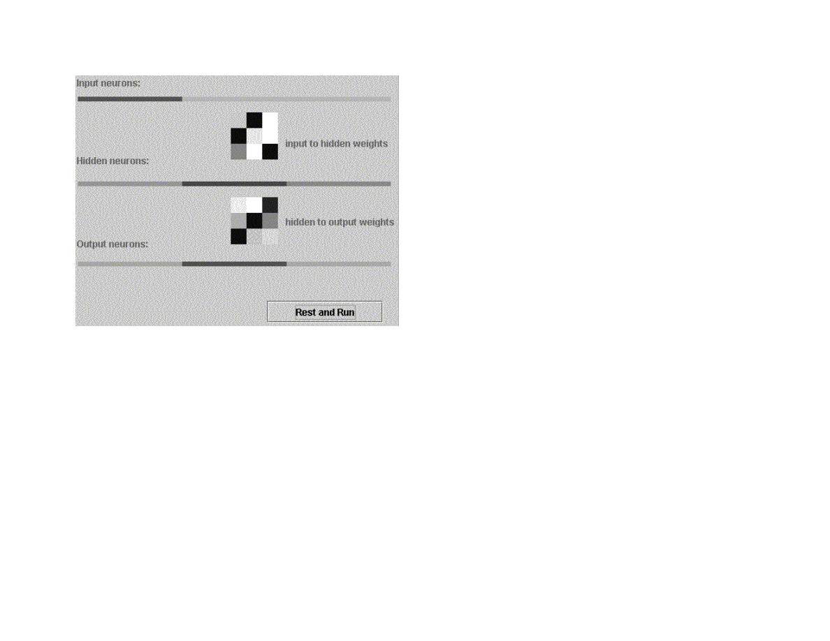
100
Figure 5.7 A one hidden layer back propagation neural network using the GUI test program GUITest_Neural_1H.java
Although back propagation networks with two hidden layers are more capable (see Figure 5.5) than networks with only one hidden
layer, I recommend always trying a one hidden layer network first for your applications. Two hidden later networks generally take a
lot longer to train and require slightly more execution time during recall.
For cases where a two hidden layer network is required, use the class Neural_2H instead of Neural_1H. There are only two changes
required to use Neural_2H. You must add an additional constructor argument for the number of neurons in the second hidden layer
and you will have to run many more training cycles. The class Neural_2H has associated test programs Test_Neural_2H.java and
GUITest_Neural_2H.java.
The only new code in Neural_2H is an extra loops in forwardPass for zeroing out the second hidden layer error array and handling
the additional hidden layer. There is also some additional code for back propagating errors to the new hidden layer in the method
train. The interested reader can read the code in Neural_2H.java. Figure 5.8 shows the GUI test program GUITest_Neural_2H
running.
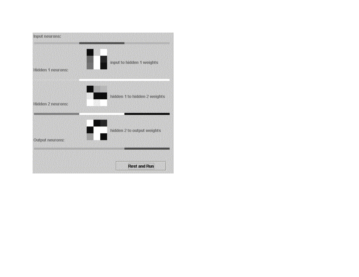
101
Figure 5.8 A two hidden layer back propagation neural network
Note (3/11/2004): I just tried running these examples under the JDK 1.4.2 and the graphics do not update until after the run is
over. To be done: fix graphics test code for a real time display)
5.7 Solving the XOR Problem
On 3/11/2004, I added a test program xor.java that solves the XOR problem. This is a more difficult problem to solve, especially when
not using “momentum” (which we are not in this chapter). However, there is another standard way to solve difficult back propagtion
problems: loop over creating new random weights and performing back propagation learning until the error is below a desired
threshold. Here is the test code in xor.java that does this iteration:
// loop until we get a low enough error:

102
try_again: for (int iter = 0; iter < 500; iter++) {
nn.randomizeWeights();
System.out.println(
"\nStarting with a new random set of weights (iter="+iter+")");
float weightJiggleFactor = 0.15f;
double learningRate = 0.4; // 0.15;
float error = 0;
for (long i = 0; i < 2000000; i++) {
nn.setLearningRate((float) learningRate);
learningRate *= 0.999995;
if (learningRate < 0.08f) learningRate = 0.08f;
error += nn.train();
if (i>0 && i % 100 == 0) {
error /= 100;
// test to see if this set of initial random weights is
// producing poor results - if so, bail and start
// with a new set of weights:
if (i > 30000 & error > 0.38f) continue try_again;
if (i > 90000 & error > 0.28f) continue try_again;
if (i >150000 & error > 0.21f) continue try_again;
if (i >350000 & error > 0.18f) continue try_again;
// if the error is low enough, simply stop training now:
if (error < 0.1) break try_again;
error = 0;
}
}
}
Here, the constants for testing how low the eror rate is were determined empirically by watching the learning process for an early
XOR training run. These checks considerably speed up this program because initial random weight sets that are not training well are
discarded early.
5.8 Notes on using back propagation neural networks
Effectively using back propagation neural networks in applications is somewhat of an acquired art. The following ad hoc notes are
derived from my experience of using neural networks over the last 16 years:
Get as much training data as possible: an effective neural network has the ability to generalize from training data, usually in the sense
of ignoring noise and spurious training examples. For this to occur, you might need thousands of training examples, depending on the
complexity of the problem. Also, some training data can be set aside (i.e., not used for training) and saved for testing the network.
For very large training data sets, try using only 10% of the data initially for training. After the output errors are small, add in more
training data sets; repeat this process until training on the entire training data set produces small errors.

103
Do not use too many hidden layer neurons: if there are too many hidden layer neurons, then the network will not learn to generalize,
rather, it will just remember all of the training data, including noise and bad training examples. Start with a very small number of
hidden neurons, and see if the training data set can be learned with very small output errors; if necessary, slowly increase the number
of hidden neurons, and repeat the training process.

104
6. Machine Learning using Weka
Note that I reused the material in this chapter of my free web book in my recent Java J2EE tchnologies book (“Sun ONE Servcies”,
M&T Press, 2001) where I cover Weka and this example with additional material. The example files for this chapter are in the
directory:
src
src/expertsystem
src/expertsystem/weka
6.1 Using machine learning to induce a set of production rules
While the topic of machine learning is not covered directly in this book (see [Witten and Frank, 1999] for a good introduction to
machine learning), we will use the Weka machine learning software package described in [Witten and Frank, 1999] as a “black box”
for generating rules for expert systems. Weka is available under a GPL license on the web at
http://www.cs.waikato.ac.nz/ml/weka
.
The techniques of machine learning have many practical applications; one example is shown in this section.
Weka supports several popular machine-learning techniques for automatically calculating classification systems. Some of the learning
algorithms supported by Weka are listed here (see [Witten and Frank, 1999, chapter 8] for a complete list):
Naïve Bayes – uses Bayes’s rule for probability of a hypothesis given evidence for the hypothesis
Instance-based learner – store all training examples and use the closest training example to classify a new data item
C4.5 – a learning scheme by J Ross Quinlan that calculates decision trees from training data. It is also possible to induce rules
from training data that are equivalent to decision trees for the same training data
Linear regression – uses training data with numeric attributes. The learned model uses linear combinations of attribute values for
classification.
Weka uses training data files in the ARFF format. This format specifies what attributes are allowed for a specified relation as well as
the data type of each attribute (i.e., character string or numeric value). We will specify a test ARFF file later in the next section; the
format is simple enough to be self-explanatory.
Our example will use Quinlan’s C4.5 learning algorithm, with a special Weka option to output rules instead of a decision tree. We will
list both the C4.5 generated rules later in a Section 6.3 after we discuss the sample problem.

105
One of the most practical aspects of machine learning is that it helps us to recognize patterns in data. The example seen in the next
section shows how a learning system like Weka can detect patterns in data that we can often exploit by writing rules that take
advantage of patterns detected by automated learning systems. Learning systems like C4.5 produce decision trees that can be easily
implemented in Java or produces equivalent rule sets that can be easily translated into rule languages like CLIPS/Jess.
6.2 A sample learning problem
We will use as training data a small set of stock market buy/sell/hold suggestions. Please note that this will be a simple demonstration
system and is not recommended for use in stock trading! We start using Weka for machine learning by selecting a learning mode (C4.5
here), designing a relation to represent the problem at hand, prepare training data, running Weka, and then interpreting/using the
results.
The first time that I set up this example system, I used a relation name stock with the following attributes (all numeric, except for the
last attribute):
last_trade – this is the current stock price
percent_change_since_open – the percentage difference between the current price and the opening price today
day_low – the lowest price so far today
day_high – the highest price so far today
action – legal values: buy, sell, or hold
The results of the trained system were bad because rules were defined for testing for the absolute value of a stock based on specific
stock pries in the training data. As a result of this experiment, I decided to make all numeric attributes relative to the opening stock
price. I ended up using the following attributes:
percent_change_since_open – the percentage difference between the current price and the opening price today
percent_change_from_day_low – the lowest price so far today
percent_change_from_day_high – the highest price so far today
action – legal values: buy, sell, or hold
There are many other reasonable attributes that we might use, but these five attributes are sufficient for a demo program. We could
have included the stock ticker name (e.g., “MSFT” for Microsoft, “SUNW” for Sun Microsystems, etc.), but this would cause Weka to
use the stock name in building the decision tree and rule set. The first four attributes are all numeric values. The last attribute is the
buy/sell/hold action on the stock. Listing 6.1 shows the file training_data.arff that is in the directory src/expertsystem/weka. There

106
are three sections in an ARFF file: relation name, attribute specification, and data. Key words @relation, @attribute, and @data have
special meaning to define sections. The keyword real implies that an attribute takes on a numeric value. The attribute action can have
one of three values specified in a set.
Listing 6.1
@relation stock
@attribute percent_change_since_open real
@attribute percent_change_from_day_low real
@attribute percent_change_from_day_high real
@attribute action {buy, sell, hold}
@data
-0.2,0.1,-0.22,hold
-2.2,0.0,-2.5,sell
0.2,0.21,-0.01,buy
-0.22,0.12,-0.25,hold
-2.0,0.0,-2.1,sell
0.28,0.26,-0.04,buy
-0.12,0.08,-0.14,hold
-2.6,0.1,-2.6,sell
0.24,0.25,-0.03,buy
6.3 Running Weka
Although Weka is a complex system, it is simple to use when using default settings. I assume that you have installed Weka on your
system (i.e., you have the weka.jar file on your system and that either your CLASSPATH contains this jar file, or the Weka jar file is in
the JDK/jre/lib/ext directory on your system). The directory src/expertsystem/weka contains two batch files:
weka_decision_tree.bat – runs Weka using C4.5 learning algorithm to produce a decision tree from the training data
weka_rules.bat – runs Weka using C4.5 learning algorithm to produce a set of ordered rules that is equivalent to a decision tree
Both of these batch files (that are Windows specific but can be trivially changed to UNIX shell files) use the “-t” option to specify the
input ARFF training file. The generate decision tree produced when running weka_decision_tree.bat is equivalent to:
If percent_change_from_day_low <= 0.12 then
if percent_change_since_open <= -2 then sell
else hold
else buy

107
Admittedly, this is a very simple decision tree, but it does show how the C4.5 learning algorithm in Weka finds patterns in data that we
can use. The ordered set of three rules generated from running the weka_rules.bat command file is:
percent_change_from_day_low <= 0.12 AND
percent_change_since_open <= -2: sell
percent_change_since_open <= =0.12: hold
: buy
These rules must be evaluated in this order to be equivalent to the generated decision tree.

108
Chapter 7. Statistical Natural Language Processing
In Chapter 2, we experimented with ATN based parsers that produced the syntactic structure of input text. We will take a very different
approach in this chapter: we will use word use statistics to assign word type tags to each word in input text. We will look in some
detail at one of the most popular approaches to tagging text: building Hidden Markov Models (HMM) evaluating these models to
assign tags to words.
A complete coverage of the techniques for training HMM is beyond the scope of this chapter. A full reference for these training
techniques is (Manning, Schutze, 1999). We will discuss the training algorithms and discuss sample Java code that implements HMM.
Advertisement
The author has written several commercial natural language processing tools that are available for purchase at www.markwatson.com.
The example in this chapter is purposely pendantic: it is intended to be easy to understand and experiment with.
7.1 Hidden Markov Models
In Hidden Markov Models HMM), we speak of an observable sequence of events that move a system through a series of states. We
attempt to assign transition probablities based on the recent history of states of the system (or, the last few events).
As an example, suppose that we want to develop a HMM that attempts to assign part of speech tags to English text. To train a HMM,
we will assume that we have a large set of training data that is a sequence of words and a parallel sequence of manually assigned part
of speech tags.
For developing a sample Java program to learn how to train a HMM, we assume that we have two Java vectors words and tags that are
of the same length.
Once the HMM is trained, we will write another Java example program that takes as input a Java vector of words and returns a Java
vector of calculated part of speech tags.
We will describe the assumptions made for Markov Models and Hidden Markov Models using this part of speech tagging problem as
an example. First, assume that the desired part of speech tags are an observable sequence:
109
t[1], t[2], t[3], ..., t[N]
and the original word sequence:
w[1], w[2], w[3], ..., w[N]
We will also assume that the probability of tag t[M] having a specific value is only a function of:
t[M-1]
and:
w[M] and w[M-1]
In some applications, instead of using the last observed state, we might use just the last two states.
For our example, we will assume that we have a finite lexicon or words and furthermore, we will use a hash table that uses the words
in the lexicon as keys and the values are the possible parts of speech the lexicon entry.
For example, assuming the lexicon hash table is named lexicon, we use the notation:
lexicon[“a-word”] -> list of possible tags.
The following table shows the possible tags used in our example system:
Tag name
Part of speech
VB
verb
NN
noun
ADJ
adjective
DT
determiner
ADV
adverb
IN
preposition
NNP
proper noun
Then, for example, we might have a lexicon entry:

110
lexicon[“bank”] -> NN, VB
where the work “bank” could be a noun (“I went to the bank”) or a verb (“To turn, bank the airplane”).
7.2 Training Hidden Markov Models
In the next two sections, we will be using code in the file Markov.java that is in the src/nlp/Markov directory. This would be a good
time to open this file in your favorite text editor of Java IDE and to take a quick look at it. We will list snippets of the code in
Markov.java in this section and Section 7.2 but it would be useful to have the full source code available when you read the following
material. In the following text, I will frequently refer to variable names and methods defined in Markov.java. The good news is that
Markov.java is only a few hundred lines long and is reasonably easy to understand.
In order to train a Markov model to tag parts of speech, we start by building a two-dimensional array
tagToTagTransitionCount[uniqueTagCount][uniqueTagCount] where the first index if the index of tag0 and the second index is
the index of tag1. The values in this two-dimensionl array will eventually indicate probabilities of transitioning from one tag to
another; at first however, we simply use this array ofr counting transitions between pairs of tags.
The element tagToTagTransitionCount[indexTag0][indexTag1] is incremented whenever we find a transition of tag0 to tag1 in the
input training text. The example program writes a spreadsheet style CSV file for this and other two dimensional arrays that are useful
for viewing intermediate training results in any spreadsheet program.
Figure 7.1 Transition counts from the fisrt tag (shown in row) to the second tag (shown in column). We see that the transition
from NNP to VB is common.
Next, we normalize the data seen in Figure 7.1 by dividing each element by the count of the total number of tag (as seen in row in
Figure 7.1). This normalized data can be seen in Figure 7.2.
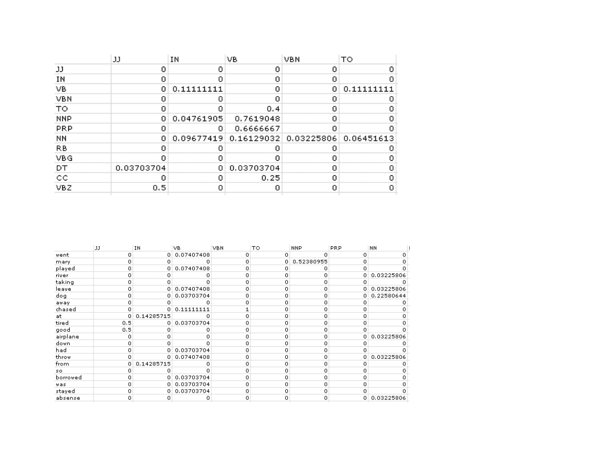
111
Figure 7.2 Normalize data in Figure 7.1 to get probability of one tag (seen in row) transitioning to another tag (seen in column)
Finally, we complete the training by defining the array probabilityWordGivenTag[uniqueWordCount][uniqueTagCount] which shows
the probability of a tag at index N producing a word at index N in the input training text. This array is seen in Figure 7.3.
Figure 7.3 Probabilities of words having specific tags

112
7.3 Using the trained Markov model to tag text
From Section 7.2, we have the probabilities of a given tag being assigned to words in the lexicon and we have the probability of a
given tag, given the preceeding tag. We will use this information in a “brute force” way: we will iterate through all possible tagging
possibilities and rate them using the formula (from [Manning/Schutze, 1999] page 347):
Rating = Product-sum(P(word|tag) * P(tag(i)|tag(i-1))
Here, P(word|tag) is the probability “word” having the tag value “tag” and P(tag(i)|tag(i-1)) is the probability of tag(i) following tag(i-
1). The arrays for these probabilities in Markov.java are probabilityWordGivenTag and probabilityTag1ToTag2. The logic for
scoring a specific tagging possibility for a sequence of words in in the method score.
The method incrementIndices is responsible for generating the next possible tagging for a sequence of words. Each word in a
sequence can have one or more possible tags. The method incrementIndices counts with a variable base per digit position. For
example, if we had four words in an input sequence with the first and last words only having one possible tag value and the second
having two possible tag values and the third word having three possible tag values, then incrementIndices would count like this:
0 0 0 0
0 1 0 0
0 0 1 0
0 1 1 0
0 0 2 0
0 1 1 0
The generated indices (i.e., each row in this listing) are stored in the class instance variable indices which is used in method score.
The method exponential_tagging_algorithm is the top level API for tagging words. Please note that the word sequence that you pass
to exponential_tagging_algorithm must not contain any words that were not in the original training data (i.e., in the file
tagged_text.txt).
We are not using an efficient algorithm if the word sequence is long. In practice this is not a real problem because you can break up
long texts into smaller pieces for tagging; for example, you might want to tag just a few sentences at a time.
The training and tagging code in Markov.java is simple. It is intended to be a short example of using Markov models.

113
Chapter 8. Bayesian Networks
Bayesian networks are used to manage complexity when dealing with known and unknown things. In real world situations, we seldom
have complete information to solve a problem.
Bayesian networks deal with probabilities associated with values of random variables.
<< TBD – after example programs are finished >>

114
Bibliography
“Data Mining”, Ian Witten and Eibe Frank, 1999, Morgan Kaufmann Publishers
Brownston, Lee, Robert Farrell, Elaine Kant, and Nancy Martin. 1985. Programming Expert Systems in OPS5. Reading, MA:
Addison-Wesley.
“Genetic Programming”, John Koza, 1992, The MIT Press
“Genetic Programming II”, John Koza, 1994, The MIT Press
Goldberg, David E. 1989. Genetic Algorithms. Reading, MA: Addison-Wesley.
“C++ Power Paradigms” Mark Watson, McGraw-Hill 1995. (Covers constraint programming, neural netowrks, and genetic
algorithms)
“Parallel Distributed Processing” volumes I and II, David E. Rumelhart, James L. McClelland, and the PDP Research Group, MIT
Press, 1986.
“Impossible Minds”, Igor Aleksander, 1996, Imperial College Press.
“Artificial Intelligence”, Elaine Rich and Kevin Knight, 1991, McGraw-Hill
“Intelligent Java Applications”, Mark Watson, 1997, Morgan Kaufmann Publishers
“Inside Computer Understanding”, Roger Schank and Christopher Riesbeck, 1981, Lawrence Erlbaum Associates Publishers
“Inside Case-Based Reasoning”, Christopher Riesbeck and Roger Schank, 1989, Lawrence Erlbaum Associates Publishers
“Reasoning About Plans”, James Allen, Henry Kautz, Richard Pelavin, and Josh Tenenberg, 1991, Morgan Kaufmann Publishers
“The Web of Life”, Fritjof Capra, 1996, Anchor Books
“Common Lisp Modules, Artificial Intelligence in the Era of Neural Networks and Chaos Theory”, Mark Watson, 1991, Springer-
Verlag

115
“Programming in Scheme, Learn Scheme through Artificial Intelligence Programs”, Mark Watson, 1996, Springer-Verlag
“Foundations of Statistical Natural Language Processing”, Christopher D. Manning and Hinrich Schutze, The MIT Press, 1999.

116
Index
A
alpha-beta search...................................................................................................... 26
ARFF format.......................................................................................................... 106
ATN parsers................................................................................................... ..........45
B
back propagation neural networks............................................................................ 93
backward chaining......................................................................................... ..........65
breadth first search................................................................................................ ...25
C
C4.5........................................................................................................ ...............107
chess program................................................................................................. .........36
chromosome............................................................................................................. 76
CLIPS............................................................................................................ ..........62
connection................................................................................................................ 93
crossover operation.......................................................................................... ........79
E
expert systems.......................................................................................................... 62
F
fitness....................................................................................................................... 78
forward chaining................................................................................................ ......64
G
GA................................................................................................................. ..........76
generation................................................................................................... .............76
genetic algorithms.................................................................................................. ..76
Gnu Public License................................................................................................ ....6
H
Hidden Markov Models......................................................................... ................110
Hopfield neural networks...................................................................................... ...88
I
input neurons........................................................................................... ................93
J
Jess........................................................................................................ ..................63
L
learning rate................................................................................................... ..........95
M
machine learning.................................................................................................. ..106
N
Natural Language Processing.................................................................................. .44
neural networks........................................................................................................ 87
NLP......................................................................................................... ................44
O
OPS5........................................................................................................................ 62
output neurons........................................................................................ .................93
P
population........................................................................................................ ........76
Prolog....................................................................................................... ...............56
Prolog (embedded)................................................................................................... 59
S
search..................................................................................................................... ..10
search tree.......................................................................................................... ......10
Sigmoid function.................................................................................. ...................94
Statistical Natural Language Processing............................................. ...................110
supervised learning..................................................................................... .............87
T
tic-tac-toe........................................................................................................... ......26
U
Unified Modeling Language.......................................................................... ............7
W
Weka.............................................................................................................. ........107
working memory..................................................................................................... .63
Wyszukiwarka
Podobne podstrony:
więcej podobnych podstron