Steady State Heat Conduction — Example
FE Analysis in 2D
Małgorzata Stojek
Cracow University of Technology
April 2013
MS
(L-53 CUT)
Heat Conduction in 2D
04/2013
1 / 30
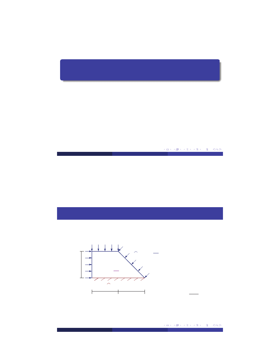
Example — Steady State Heat Transfer
T=500 [K]
q=100
m
2
W
[ ]
m
[ ]
W
3
f=120
1
1
1
κ
=
1
h
W
m deg
i
MS
(L-53 CUT)
Heat Conduction in 2D
04/2013
2 / 30
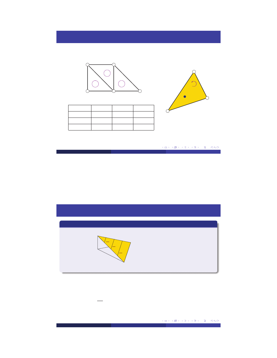
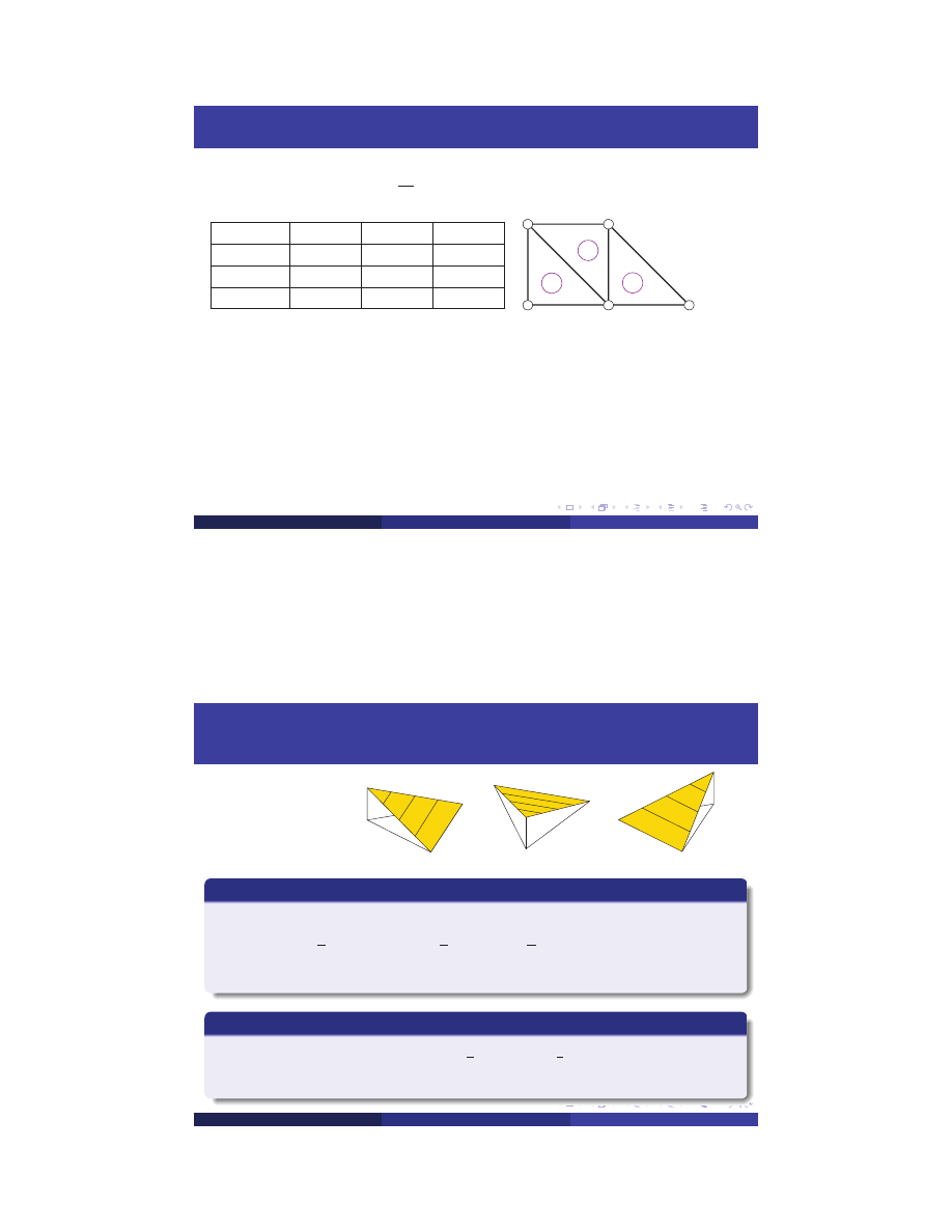
FE Discretization
1
2
3
1
2
4
3
5
no elem.
node 1
node 2
node 3
1
1
2
4
2
4
3
1
3
3
4
5
T
3
T
2
T
1
T(x,y)
MS
(L-53 CUT)
Heat Conduction in 2D
04/2013
3 / 30
Element Shape Functions
Fact
1
ζ
1
N =
1
2
4
1
4
3
1
2
3
1
0
N
1
+
N
2
+
N
3
=
1
N
1
N
2
N
3
=
1
2A
det
x
2
x
3
y
2
y
3
y
2
−
y
3
x
3
−
x
2
det
x
3
x
1
y
3
y
1
y
3
−
y
1
x
1
−
x
3
det
x
1
x
2
y
1
y
2
y
1
−
y
2
x
2
−
x
1
1
x
y
MS
(L-53 CUT)
Heat Conduction in 2D
04/2013
4 / 30
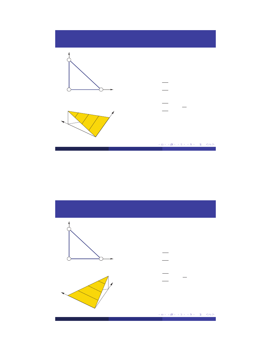
Shape Functions - Element no 1
First Node
(0,0)
2
3
x
1
y
(0,1)
(1,0)
1
N =y
1
2
3
y
x
B
1
= ∇
N
1
=
∂
N
1
∂
x
∂
N
1
∂
y
!
=
0
1
!
B
1
= ∇
N
1
=
∂
N
1
∂
x
∂
N
1
∂
y
!
=
1
2A
y
2
−
y
3
x
3
−
x
2
!
MS
(L-53 CUT)
Heat Conduction in 2D
04/2013
5 / 30
Element Shape Functions - Element no 1
Third Node
(0,0)
2
3
x
1
y
(0,1)
(1,0)
3
N =x
1
2
3
y
x
B
3
= ∇
N
3
=
∂
N
3
∂
x
∂
N 3
∂
y
!
=
1
0
!
B
3
= ∇
N
3
=
∂
N
3
∂
x
∂
N 3
∂
y
!
=
1
2A
y
1
−
y
2
x
2
−
x
1
!
MS
(L-53 CUT)
Heat Conduction in 2D
04/2013
6 / 30
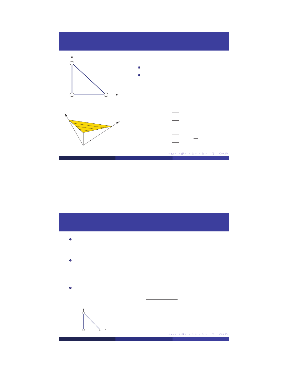
Element Shape Functions - Element no 1
Second Node
(0,0)
2
3
x
1
y
(0,1)
(1,0)
2
N =1-x-y
y
1
2
3
x
N
2
=
1
−
N
1
−
N
3
N
2
=
a
0
+
a
1
x
+
a
2
y
(
0, 0
)
1
=
a
0
(
0, 1
)
0
=
1
+
a
2
→
a
2
= −
1
(
1, 0
)
0
=
1
+
a
3
→
a
3
= −
1
B
2
= ∇
N
2
=
∂
N
2
∂
x
∂
N
2
∂
y
!
=
−
1
−
1
!
B
2
= ∇
N
2
=
∂
N
2
∂
x
∂
N
2
∂
y
!
=
1
2A
y
3
−
y
1
x
1
−
x
3
!
MS
(L-53 CUT)
Heat Conduction in 2D
04/2013
7 / 30
Element Shape Functions - Element no 1
Second Node - Third Method
edge
13
:
y
=
ax
+
b
→
0
= −
y
−
ax
+
b
edge
13
⊂
plane
z
(
x, y
) = −
y
−
ax
+
b for
z
(
x
1
, y
1
) =
0
z
(
x
3
, y
3
) =
0
N
2
⊂
z
(
x, y
) = −
y
−
ax
+
b (compact support &
z
(
x
2
, y
2
) =
1
)
N
2
(
x, y
) = −
y
−
ax
+
b
−
y
2
−
ax
2
+
b
(0,0)
2
3
x
1
y
(1,0)
(0,1)
y=-x+1
N
2
=
−
y
−
x
+
1
−(
0
) − (
0
) +
1
=
1
−
x
−
y
MS
(L-53 CUT)
Heat Conduction in 2D
04/2013
8 / 30

Element Stiffness Matrix I
(0,0)
2
3
x
1
y
(0,1)
(1,0)
N
1
N
2
N
3
B
1
B
2
B
3
y
1
−
x
−
y
x
0
1
!
−
1
−
1
!
1
0
!
K
e
ij
=
κ
R
Ω
e
(
B
i
)
T
B
j
d Ω
→
K
e
ij
=
κ
(
B
i
)
T
B
j
Z
Ω
e
d Ω
=
κ
2
(
B
i
)
T
B
j
K
e
11
=
κ
2
0 1
0
1
!
=
κ
2
K
e
12
=
κ
2
0 1
−
1
−
1
!
= −
κ
2
. . .
K
e
=
κ
2
1
−
1
0
−
1
2
−
1
0
−
1
1
NOTE:
X
T
X
=
X
·
X
MS
(L-53 CUT)
Heat Conduction in 2D
04/2013
9 / 30
Element Stiffness Matrix II
K
e
=
κ
R
Ω
e
(
B
e
)
T
B
e
d Ω
B
e
=
B
1
B
2
B
3
=
0
−
1 1
1
−
1 0
K
e
=
κ
2
0
1
−
1
−
1
1
0
0
−
1 1
1
−
1 0
K
e
=
κ
2
1
−
1
0
−
1
2
−
1
0
−
1
1
MS
(L-53 CUT)
Heat Conduction in 2D
04/2013
10 / 30
Element Stiffness Matrix III
B
e
=
B
1
B
2
B
3
=
1
2A
y
2
−
y
3
y
3
−
y
1
y
1
−
y
2
x
3
−
x
2
x
1
−
x
3
x
2
−
x
1
no elem.
node 1
node 2
node 3
1
1
2
4
2
4
3
1
3
3
4
5
1
2
3
1
2
4
3
5
K
e
=
κ
Z
Ω
e
(
B
e
)
T
B
e
d Ω
=
κ
A
(
B
e
)
T
B
e
K
e1
=
K
e3
B
e2
= −
B
e1
=⇒
K
e2
=
K
e1
MS
(L-53 CUT)
Heat Conduction in 2D
04/2013
11 / 30
Element Load Vector
General Remarks
F
e
=
F
e
f
+
F
e
BC
1
N
1
2
3
2
N
1
2
3
3
N
1
2
3
Fact
Z
Ω
e
N
e
i
d Ω
=
1
3
·
h
·
Z
Ω
e
d Ω
=
1
3
·
h
·
A
e
=
1
3
A
e
( tetrahedron’s volume)
Fact
one edge L
12
:
I
nod 2
nod 1
N
e
i
ds
=
1
2
·
h
·
L
12
=
1
2
L
12
i
=
1, 2
0
i
=
3
MS
(L-53 CUT)
Heat Conduction in 2D
04/2013
12 / 30

Element Load Vector
Internal Heat Supply (Constant Rate)
f
=
120
W
m
3
,
∀
e
i
A
e
i
=
1
2
m
2
F
e
f
=
Z
Ω
e
(
N
e
)
T
f
d Ω
=
f
Z
Ω
e
N
1
d Ω
Z
Ω
e
N
2
d Ω
Z
Ω
e
N
3
d Ω
=
f
A
e
1
3
1
3
1
3
F
e1
f
=
F
e2
f
=
F
e3
f
=
120
·
1
2
·
1
3
1
3
1
3
=
20
20
20
MS
(L-53 CUT)
Heat Conduction in 2D
04/2013
13 / 30
Element Load Vector
Constant Inward Heat Flux
bq
=
100
W
m
2
=⇒
F
e
BC
=
Z
∂Ω
e
N
(
N
e
)
T
bq
ds
=
bq
Z
∂Ω
e
N
(
N
e
)
T
ds
(1,0)
1
(0,1)
(0,0)
2
3
1
2
(1,1)
(1,0)
(0,1)
3
1
(2, 0)
3
(1, 1)
2
(1, 0)
100
1
2
·
1
1
2
·
1
0
100
0
1
2
·
1
1
2
·
1
100
1
2
·
√
2
0
1
2
·
√
2
F
e1
BC
=
50
50
0
F
e2
BC
=
0
50
50
F
e3
BC
=
70.7
0
70.7
MS
(L-53 CUT)
Heat Conduction in 2D
04/2013
14 / 30

Element Load Vector
load vector
elem 1
elem 2
elem 3
F
e
f
20
20
20
20
20
20
20
20
20
F
e
BC
50
50
0
0
50
50
70.7
0
70.7
F
e
=
F
e
f
+
F
e
BC
70
70
20
20
70
70
90.7
20
90.7
MS
(L-53 CUT)
Heat Conduction in 2D
04/2013
15 / 30
Assembly Process
Global Stiffness Matrix & Load Vector
no elem.
global DOFs
1
1, 2, 4
2
4, 3, 1
3
3, 4, 5
K
=
0
5
×
5
(+)
K
e1
3
×
3
(+)
K
e2
3
×
3
(+)
K
e3
3
×
3
F
=
0
5
×
1
(+)
F
e1
3
×
1
(+)
F
e2
3
×
1
(+)
F
e3
3
×
1
Before assembly:
K
=
0 0 0 0 0
0 0 0 0 0
0 0 0 0 0
0 0 0 0 0
0 0 0 0 0
,
F
=
0
0
0
0
0
MS
(L-53 CUT)
Heat Conduction in 2D
04/2013
16 / 30

Assembly Process
First Element
no elem.
global DOFs
1
1, 2, 4
K
e
1
=
κ
2
1
−
1
0
−
1
2
−
1
0
−
1
1
F
e
1
=
70
70
20
K
=
κ
2
1
−
1
0
0
0
−
1
2
0
−
1
0
0
0
0
0
0
0
−
1
0
1
0
0
0
0
0
0
F
=
70
70
0
20
0
MS
(L-53 CUT)
Heat Conduction in 2D
04/2013
17 / 30
Assembly Process
Second Element
no elem.
global DOFs
2
4, 3, 1
K
e
2
=
κ
2
1
−
1
0
−
1
2
−
1
0
−
1
1
F
e
2
=
20
70
70
K
=
κ
2
1
+
1
−
1 0
+
(−
1
)
0
+
0
0
−
1
2
0
−
1 0
0
+
(−
1
)
0
0
+
2
0
+
(−
1
)
0
0
+
0
−
1 0
+
(−
1
)
1
+
1
0
0
0
0
0 0
F
=
70
+
70
70
0
+
70
20
+
20
0
MS
(L-53 CUT)
Heat Conduction in 2D
04/2013
18 / 30

Assembly Process
Third Element
no elem.
global DOFs
3
3, 4, 5
K
e
3
=
κ
2
1
−
1
0
−
1
2
−
1
0
−
1
1
F
e
3
=
90.7
20
90.7
K
=
κ
2
2
−
1
−
1
0
0
−
1
2
0
−
1
0
−
1
0
2
+
1
−
1
+
(−
1
)
0
+
0
0
−
1
−
1
+
(−
1
)
2
+
2
0
+
(−
1
)
0
0
0
+
0
0
+
(−
1
)
0
+
1
F
=
140
70
70
+
90.7
40
+
20
0
+
90.7
MS
(L-53 CUT)
Heat Conduction in 2D
04/2013
19 / 30
Assembly Process
Global Matrix Equations
Kd
=
F
1
2
2
−
1
−
1
0
0
−
1
2
0
−
1
0
−
1
0
3
−
2
0
0
−
1
−
2
4
−
1
0
0
0
−
1
1
T
1
T
2
T
3
T
4
T
5
=
140
70
160.7
60
90.7
NOTE:
det K
=
0,
rank
(
K
) =
4
.
MS
(L-53 CUT)
Heat Conduction in 2D
04/2013
20 / 30

Essential Boundary Conditions
1
2
3
1
2
4
3
5
T
2
=
T
4
=
T
5
=
500
T
1
T
2
T
3
T
4
T
5
→
T
1
500
T
3
500
500
1
2
2
−
1
−
1
0
0
−
1
2
0
−
1
0
−
1
0
3
−
2
0
0
−
1
−
2
4
−
1
0
0
0
−
1
1
T
1
500
T
3
500
500
=
140
70
160.7
60
90.7
MS
(L-53 CUT)
Heat Conduction in 2D
04/2013
21 / 30
Solution
1
2
2
−
1
−
1
0 0
−
1
0
3
−
2 0
T
1
500
T
3
500
500
=
140
160.7
1
2
2
−
1
−
1
3
T
1
T
3
=
140
160.7
−
1
2
−
1
0 0
0
−
2 0
500
500
500
1.0
−
0.5
−
0.5
1.5
T
1
T
3
=
390
660.7
Solution is
:
T
1
T
3
=
732
685
→
d
=
T
1
500
T
3
500
500
=
732
500
685
500
500
MS
(L-53 CUT)
Heat Conduction in 2D
04/2013
22 / 30

Postprocessing
General Remarks
RECALL:
no elem.
global DOFs
1
1
,
2
,
4
2
4
,
3
,
1
3
3
,
4
,
5
,
d
=
732
500
685
500
500
temperature field
T
e
(
x, y
) =
N
e
d
e
heat flux rate
q
e
(
x, y
) = −
κ
∇
T
= −
κB
e
d
e κ
=
1
= −
B
e
d
e
MS
(L-53 CUT)
Heat Conduction in 2D
04/2013
23 / 30
Postprocessing
Element Data
N
e
B
e
= ∇
N
e
elem 1
y
1
−
x
−
y
x
0
−
1 1
1
−
1 0
elem 2
1
−
y
x
+
y
−
1 1
−
x
0 1
−
1
−
1 1
0
elem 3
y
2
−
y
−
x
x
−
1
0
−
1 1
1
−
1 0
MS
(L-53 CUT)
Heat Conduction in 2D
04/2013
24 / 30

Postprocessing
First Element
no elem.
global DOFs
1
1
,
2
,
4
,
d
=
732
500
685
500
500
temperature field
[
deg
]
T
e
1
(
x, y
) =
N
e
1
d
e
1
=
y
1
−
x
−
y
x
732
500
500
=
232y
+
500
heat flux rate
W
m
2
q
e
1
(
x, y
) = −
B
e
1
d
e
1
= −
0
−
1 1
1
−
1 0
732
500
500
=
0
−
232
MS
(L-53 CUT)
Heat Conduction in 2D
04/2013
25 / 30
Postprocessing
Second Element
no elem.
global DOFs
2
4
,
3
,
1
,
d
=
732
500
685
500
500
temperature field
[
deg
]
T
e
2
(
x, y
) =
1
−
y
x
+
y
−
1 1
−
x
500
685
732
=
185y
−
47x
+
547
heat flux rate
W
m
2
q
e
2
(
x, y
) = −
0
1
−
1
−
1 1
0
500
685
732
=
47
−
185
MS
(L-53 CUT)
Heat Conduction in 2D
04/2013
26 / 30
Postprocessing
Third Element
no elem.
global DOFs
3
3
,
4
,
5
,
d
=
732
500
685
500
500
temperature field
[
deg
]
T
e
3
(
x, y
) =
y
2
−
y
−
x
x
−
1
685
500
500
=
185y
+
500
heat flux rate
W
m
2
q
e
3
(
x, y
) = −
0
−
1 1
1
−
1 0
685
500
500
=
0
−
185
MS
(L-53 CUT)
Heat Conduction in 2D
04/2013
27 / 30
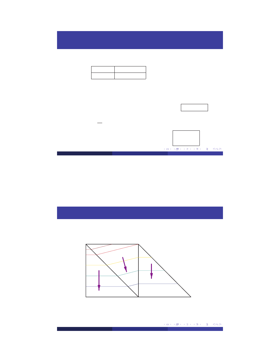
Temperature Field
500
500
500
732
708.5
685
592.5
q
q
q
MS
(L-53 CUT)
Heat Conduction in 2D
04/2013
28 / 30
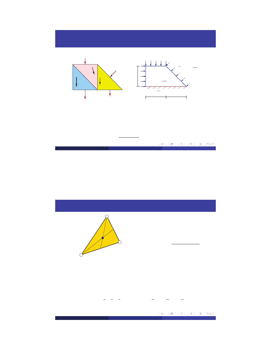
Heat Flux Rate
Heat Exchange
1 8 5 [W/m]
1 8 5 [W/m]
2 3 2 [W/m]
1 8 5 [W/m]
[0, -232]
2
4
1
3
[47, -185]
[0, -185]
5
T=500 [K]
q=100
m
2
W
[ ]
m
[ ]
W
3
f=120
1
1
1
Q
exact
L
25
= −
R
Ω
f
d Ω
+
R
∂Ω
N
bq
ds
= − (
180
+
341
) = −
521
Q
app.
L
25
= −
232
−
185
= −
417
e
L
25
=
521
−
417
521
100%
=
20%
MS
(L-53 CUT)
Heat Conduction in 2D
04/2013
29 / 30
Temperature at Element Centroid
T
3
T
2
T
1
(x ,y )
c c
T
(
x
c
, y
c
) =
T
1
+
T
2
+
T
3
3
since
T
(
x
c
, y
c
) =
N
1
(
x
c
, y
c
)
N
2
(
x
c
, y
c
)
N
3
(
x
c
, y
c
)
T
1
T
2
T
3
=
=
1
3
1
3
1
3
T
1
T
2
T
3
=
1
3
T
1
+
1
3
T
2
+
1
3
T
3
MS
(L-53 CUT)
Heat Conduction in 2D
04/2013
30 / 30
Wyszukiwarka
Podobne podstrony:
28 04 2013 cw id 31908 Nieznany
EdM wzmacniacze for stud id 150 Nieznany
07 05 2013 odwiert (1)id 6788 Nieznany
korelacja stud id 248034 Nieznany
25 3 2013 traduction id 31052 Nieznany (2)
letni 2013 I e kolo id 267392 Nieznany
28 10 2013 Geografia id 31910 Nieznany (2)
AnFinP W3 2014 stud id 63620 Nieznany (2)
oparzenia 2013 druk id 335902 Nieznany
LM SZ 01 2013 mat id 271607 Nieznany
Ekonomia stud id 283921 Nieznany
P 2013 lab P id 797792 Nieznany
Lista5 AF 2013 a1 id 270434 Nieznany
2IA PS2 2012 2013 04 B id 32601 Nieznany (2)
Lista6 AF 2013 a1 id 270468 Nieznany
Instrukcja bhp 2013 2014 id 215 Nieznany
Przetargi dla stud id 406614 Nieznany
Lista4 AF 2013 c1 id 270402 Nieznany
więcej podobnych podstron