
Lecture 9: Robust Design
Spanos
EE290H F05
1
Robust Design
A New Definition of Quality.
The Signal-to-Noise Ratio.
Orthogonal Arrays.

Lecture 9: Robust Design
Spanos
EE290H F05
2
The Taguchi Philosophy
Quality is related to the total loss to society due to
functional and environmental variance of a given product
Quality is related to the total loss to society due to
functional and environmental variance of a given product
Taguchi's method focuses on Robust Design through use of:
• S/N Ratio to quantify quality
• Orthogonal Arrays to investigate quality
Taguchi starts with a new definition of Quality:
Lecture 9: Robust Design
Spanos
EE290H F05
3
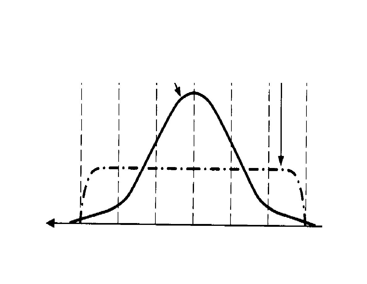
Meeting the specs vs. hitting the target
better quality
worse quality
m
m-5
m+5
Lecture 9: Robust Design
Spanos
EE290H F05
4
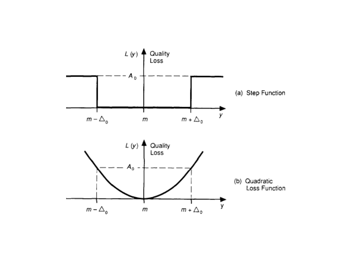
Quadratic Loss Function:
L(y) = k (y - m)
2
Fig 2.3 pp 18 from
Quality Engineering Using Robust Design
by Madhav S. Phadke
Prentice Hall 1989
Lecture 9: Robust Design
Spanos
EE290H F05
5
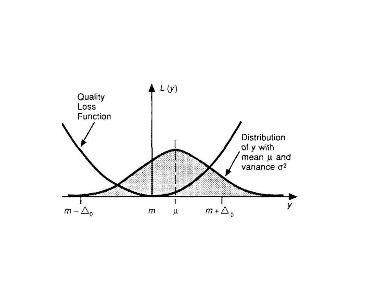
Quadratic Loss Function on Normal Distribution
Average quality loss due to µ and
σ:
Fig 2.5 pp 26
E(Q) = k [(µ-m) +
σ ]
2
2
Lecture 9: Robust Design
Spanos
EE290H F05
6
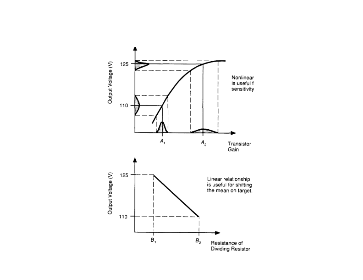
Exploiting non-linearity:
Fig 2.6 pp 28
Lecture 9: Robust Design
Spanos
EE290H F05
7
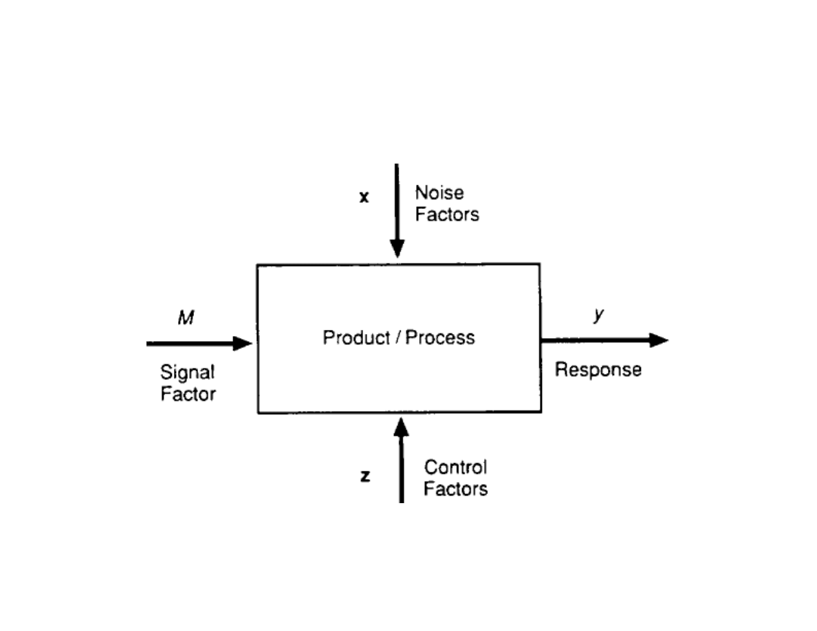
Parameters are classified according to function:
Fig 2.7 pp 30

Lecture 9: Robust Design
Spanos
EE290H F05
8
Orthogonal Arrays
b = (X
T
X)
-1
X
T
y
V(b) = (X
T
X)
-1
σ
2
During Regression Analysis, an orthogonal arrangement of
the experiment gave us independent model parameter
estimates:
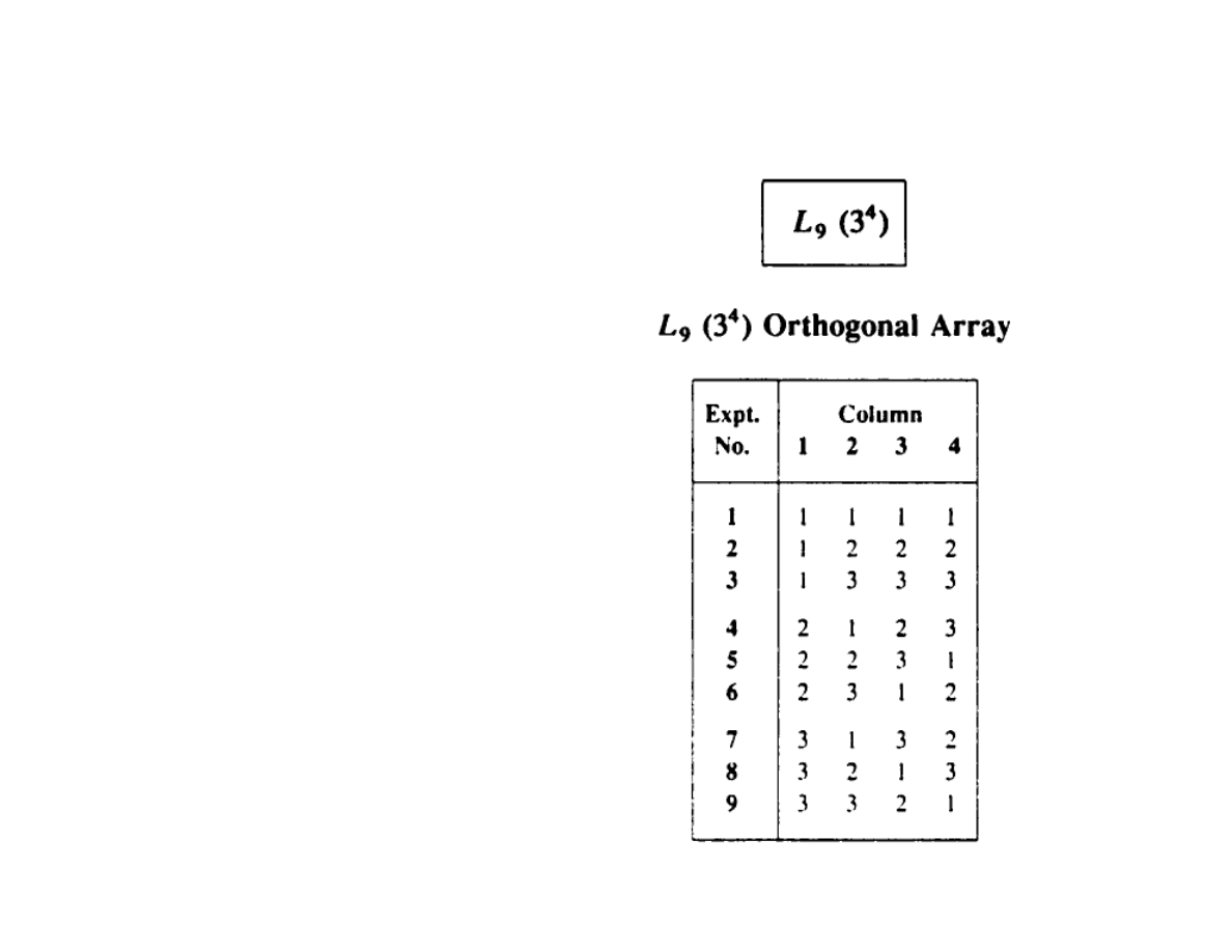
Orthogonal arrays have the same objective:
For every two columns all possible factor combinations
occur equal times.
L
4
(2
3
) L
9
(3
4
) L
12
(2
11
) L
18
(2
1
x 3
7
)
Lecture 9: Robust Design
Spanos
EE290H F05
9
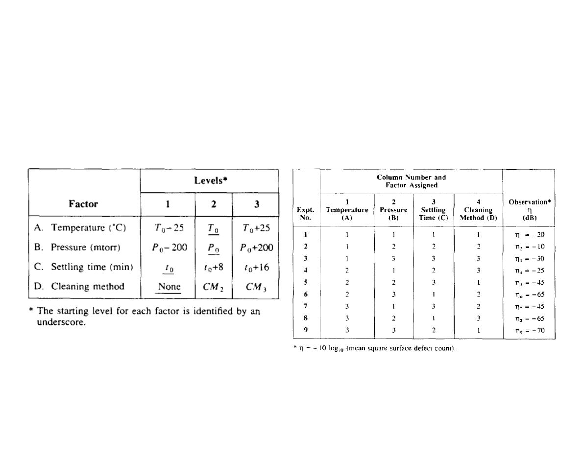
Simple CVD experiment for defect reduction
max n = -10 log (MSQ def)
10
Lecture 9: Robust Design
Spanos
EE290H F05
10
Simple CVD experiment for defect reduction (cont)
Using the L
9
orthogonal array:
Lecture 9: Robust Design
Spanos
EE290H F05
11
Estimation of Factor Effects (ANOM)
m = 1
9
η
1
+
η
2
+
η
3
+...+
η
9
m
A
1
= 1
3
η
1
+
η
2
+
η
3
m
A
2
= 1
3
η
4
+
η
5
+
η
6
m
A
3
= 1
3
η
7
+
η
8
+
η
9
...
m
B
2
= 1
3
η
2
+
η
5
+
η
8
...
m
D
3
= 1
3
η
3
+
η
4
+
η
8
η A
i
,B
j
,C
k
,D
l
= μ+α
i
+β
j
+γ
k
+δ
l
+e
α
i
= 0
Σ
β
i
= 0
Σ
γ
i
= 0
Σ
δ
i
= 0
Σ
Lecture 9: Robust Design
Spanos
EE290H F05
12
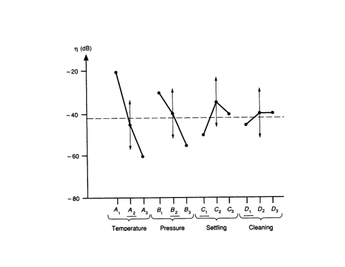
Analysis of CVD defect reduction experiment
Fig 3.1 pp 46
Tab 3.4 pp 55

Lecture 9: Robust Design
Spanos
EE290H F05
13
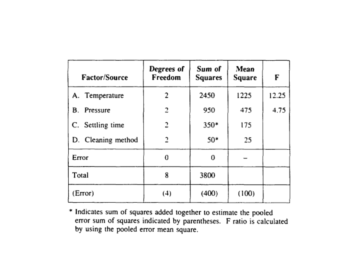
ANOVA for CVD defect reduction experiment
Grand total sum of squares:
η
i
2
= 19,425 (dB)
2
Σ
i=1
9
Total sum of squares:
η
i
-m
2
= 3,800 (dB)
2
Σ
i=1
9
Sum of squares due to mean:
m
2
= 15,625 (dB)
2
Σ
i=1
9
Sum of squares due to error:
e
i
2
= ??? (dB)
2
Σ
i=1
9
Sum of squares due to A: 3
m
A
i
-m
2
= 2,450 (dB)
2
Σ
i=1
3
Lecture 9: Robust Design
Spanos
EE290H F05
14
ANOVA for CVD defect reduction experiment (cont)

Lecture 9: Robust Design
Spanos
EE290H F05
15
Estimation of Error Variance
The experimental error is estimated from the ANOVA
residuals.
It is then used to estimate the error of the effects and to
determine their significance at the 5% level.

Lecture 9: Robust Design
Spanos
EE290H F05
16
Confirmation Experiment
Once the optimum choice has been made, it is tested by
performing a confirmation run.
This run is used to "validate" the model as well as confirm
the improvements in the process.
Variance of prediction (for the model)
σ
pred
2
=
σ
e
2
n
0
+
σ
e
2
n
r
This gives us +/-2
σ limits on the confirmation experiment.
1
n
0
σ
e
2
= 1
n +
1
n
A
1
- 1
n +
1
n
B
1
- 1
n σ
e
2
Lecture 9: Robust Design
Spanos
EE290H F05
17
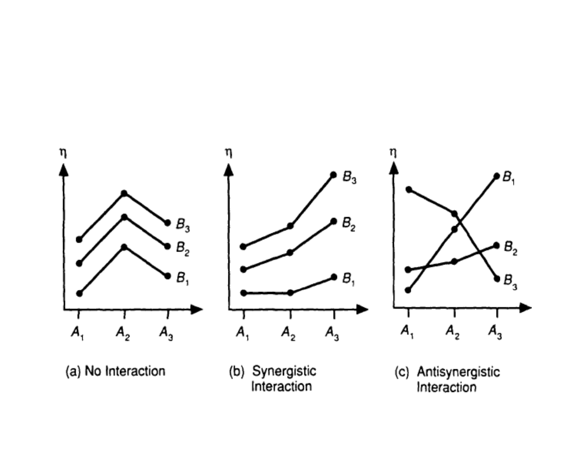
The additive model
Fig 3.3 pp 63, enlarged 120%
Since we assumed additive model, we must make sure
that there are no interactions:

Lecture 9: Robust Design
Spanos
EE290H F05
18
Example: Large CVD experiment.
Objectives:
a) reduce defects n = -10 log (MSQ Def)
b) maximize S/N of rate n'= 10 log (µ /
σ )
c) adjust poly thickness to a 3600 Å target.
10
10
2
2
Lecture 9: Robust Design
Spanos
EE290H F05
19
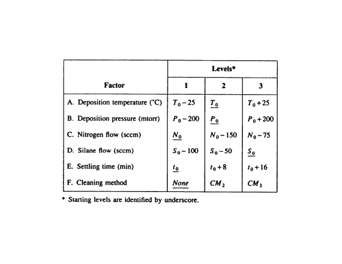
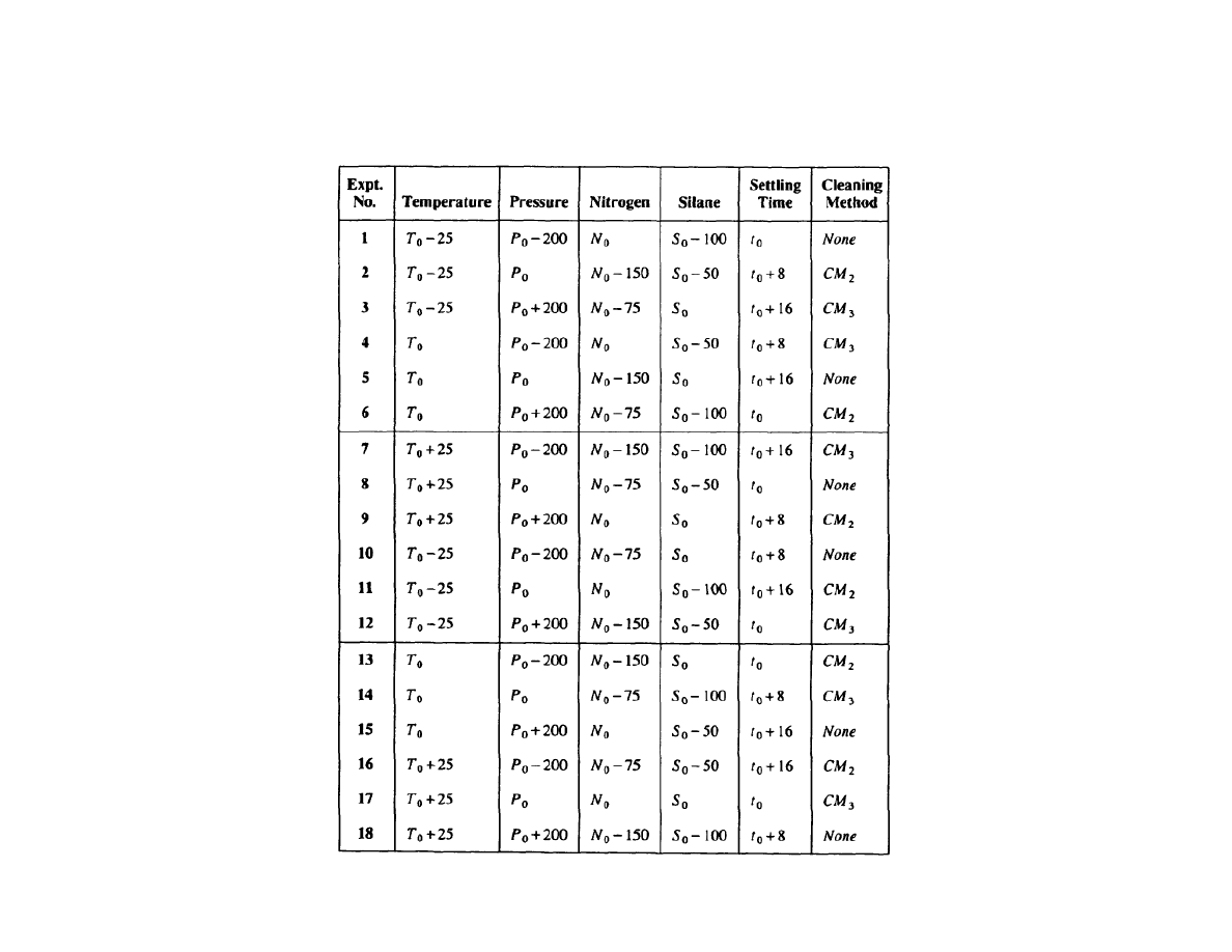
Choosing the Control Factors
Tab 4.6-7 pp 88-90
Lecture 9: Robust Design
Spanos
EE290H F05
20
Using the L
18
orthogonal array...
Tab 4.3 pp 78, enlarged 120%
Lecture 9: Robust Design
Spanos
EE290H F05
21
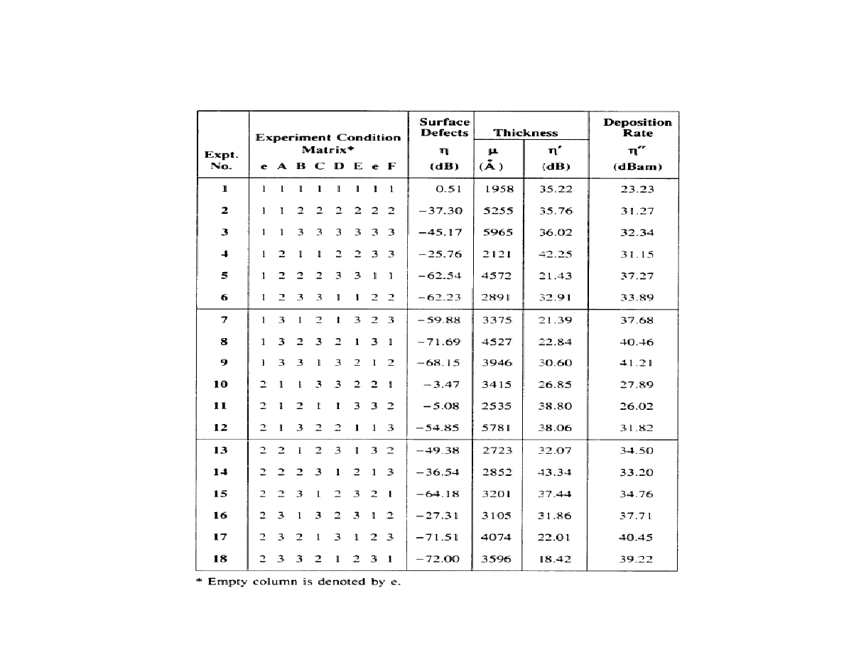
Data summary for large CVD experiment:
Tab 4.5 pp 85, enlarged 120%
Lecture 9: Robust Design
Spanos
EE290H F05
22
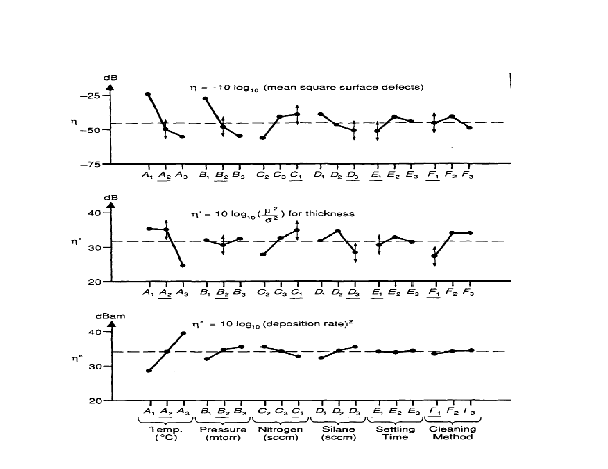
Data analysis for large CVD experiment (cont)
Fig 4.5 pp 86, enlarged 120%
Lecture 9: Robust Design
Spanos
EE290H F05
23
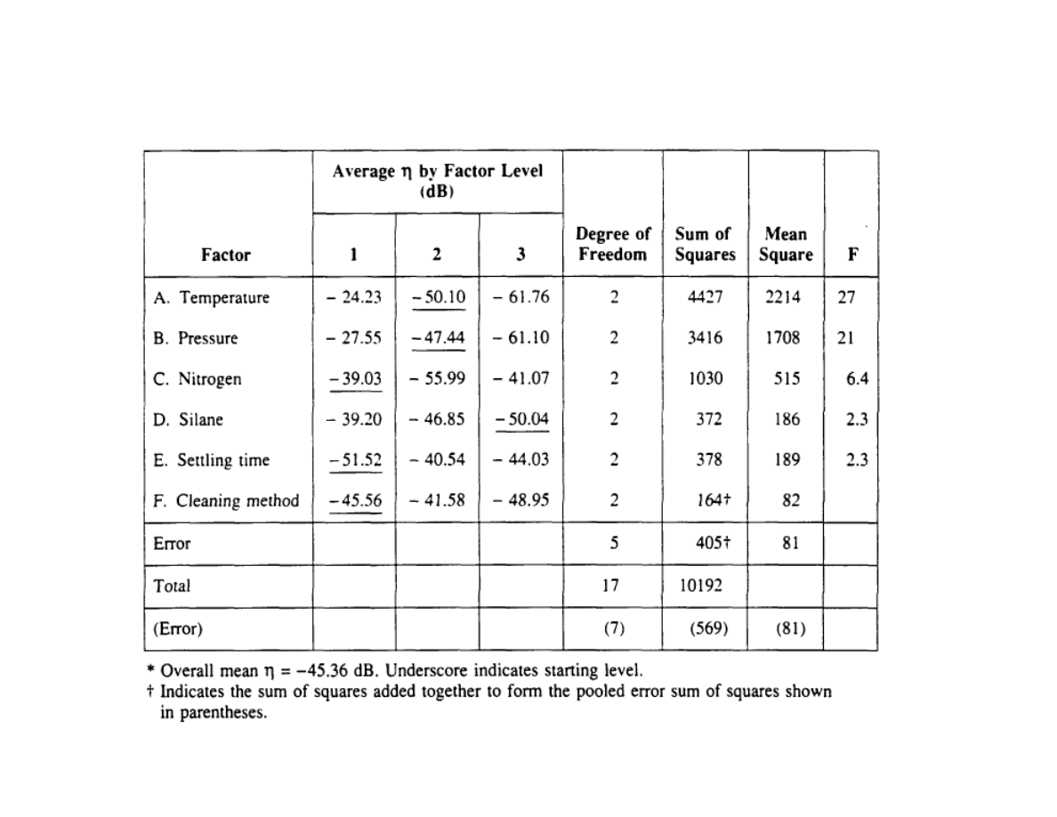
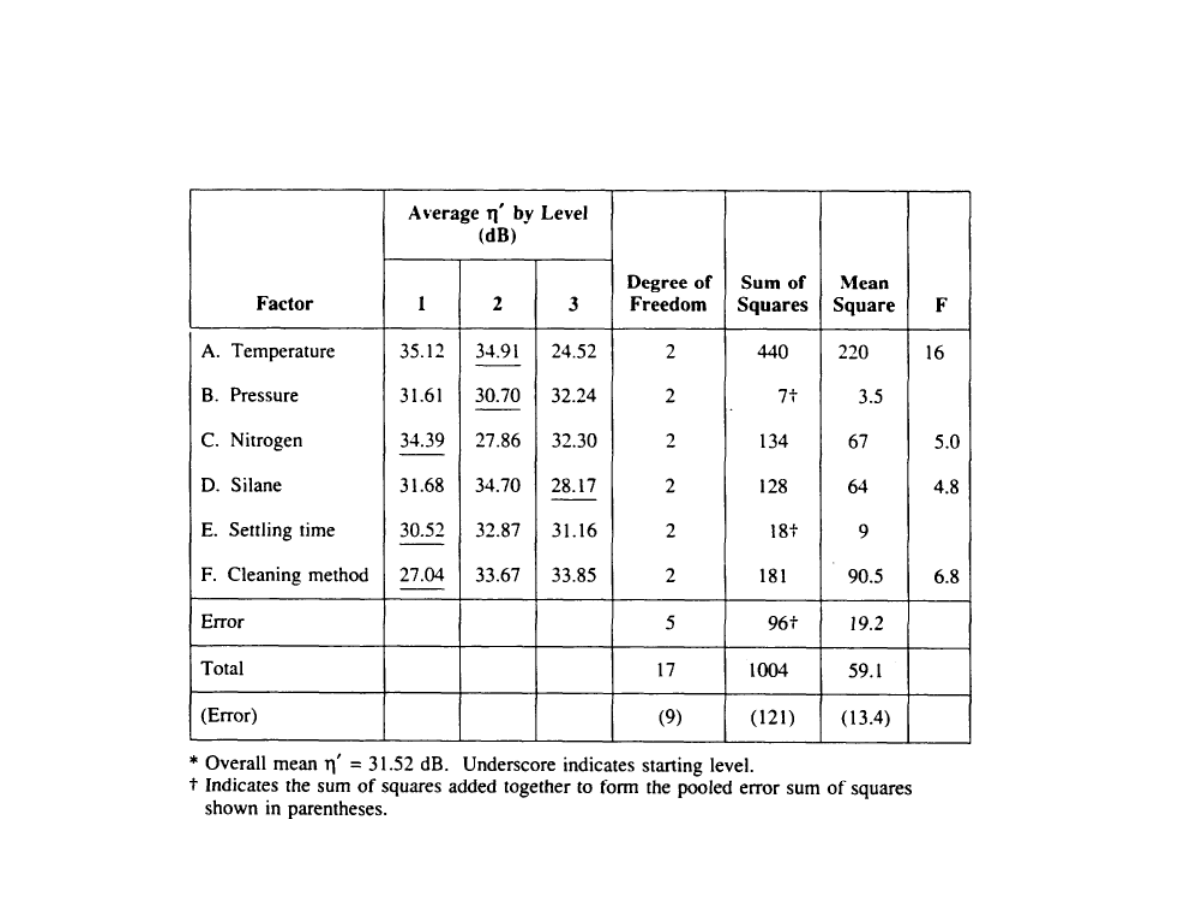
ANOVA table for large CVD experiment:
η
Lecture 9: Robust Design
Spanos
EE290H F05
24
ANOVA table for large CVD experiment :
η’
Lecture 9: Robust Design
Spanos
EE290H F05
25
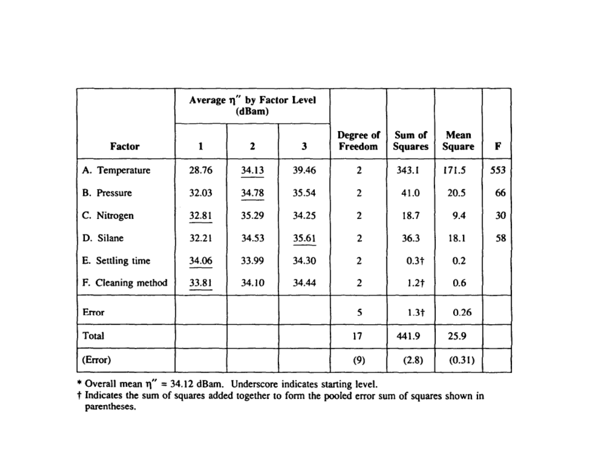
ANOVA tables for large CVD experiment:
η’’
Lecture 9: Robust Design
Spanos
EE290H F05
26
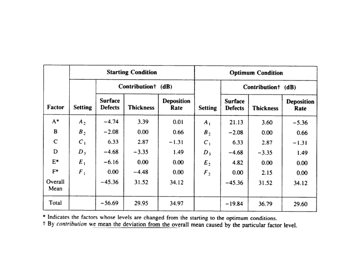
Combined Prediction Using the Additive Model
Tab 4.6-7 pp 88-90
Lecture 9: Robust Design
Spanos
EE290H F05
27
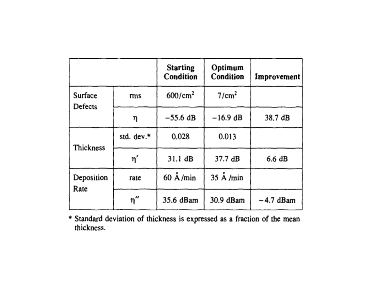
Verification for large CVD experiment
Tab 4.10-11 pp 92
for further reading: Quality Engineering Using Robust Design by Madhav S. Phadke
Prentice Hall 1989

Lecture 9: Robust Design
Spanos
EE290H F05
28
“Inner” and “Outer” Arrays
•
Often one want to improve performance based on some “control”
factors, in the presence of some “noise” factors.
•
Two arrays are involved: the inner array explores the “control”
factors, and the entire experiment is repeated across an array of the
noise factors.
•
Inner arrays are typically orthogonal designs
•
Outer arrays are typically small, 2-level fractional factorial designs.
Lecture 9: Robust Design
Spanos
EE290H F05
29
Why use S/N Ratios?
• They lead to an optimum through a monotonic function.
• They help improve additivity of the effects.
⎟
⎠
⎞
⎜
⎝
⎛
−
=
⎟⎟
⎠
⎞
⎜⎜
⎝
⎛
−
=
⎟⎟
⎠
⎞
⎜⎜
⎝
⎛
−
=
∑
∑
i
i
STB
i
i
LTB
Y
n
N
S
Y
n
N
S
s
Y
N
S
2
2
2
2
1
log
10
1
1
log
10
log
10
Nominal is best:
Larger is better:
Smaller is better:

Lecture 9: Robust Design
Spanos
EE290H F05
30
Taguchi vs. RSM
Taguchi
RSM
Small number of runs
Explicit control of Interactions
Engineering Intuition
Statistical Intuition
“Complete” package
Training Issues
Additive Models
More General Models
Orthogonal Arrays
Fractional Factorials
A “Philosophy”
A Tool
Lecture 9: Robust Design
Spanos
EE290H F05
31
Design of Experiments
Comparison of Treatments
Blocking and Randomization
Reference Distributions
ANOVA
MANOVA
Factorial Designs
Two Level Factorials
Blocking
Fractional Factorials
Regression Analysis
Robust Design
Analysis
Modeling
Wyszukiwarka
Podobne podstrony:
Australian by design id 72410 Nieznany (2)
LOW EMI PCB DESIGN id 273292 Nieznany
lecture 14 CUSUM and EWMA id 26 Nieznany
lecture05 id 264350 Nieznany
lecture8 id 264393 Nieznany
lecture3 id 264379 Nieznany
lecture7 id 264390 Nieznany
lecture5 id 264383 Nieznany
JPA Lecture2 id 228757 Nieznany
pole placement robot design id Nieznany
lecture2 id 264375 Nieznany
lecture4 id 264381 Nieznany
Abolicja podatkowa id 50334 Nieznany (2)
4 LIDER MENEDZER id 37733 Nieznany (2)
katechezy MB id 233498 Nieznany
metro sciaga id 296943 Nieznany
perf id 354744 Nieznany
interbase id 92028 Nieznany
więcej podobnych podstron