http://www.mece.ualberta.ca/tutorials/ansys/AT/NonLinear/Print.

NonLinear Analysis of a Cantilever Beam

Introduction

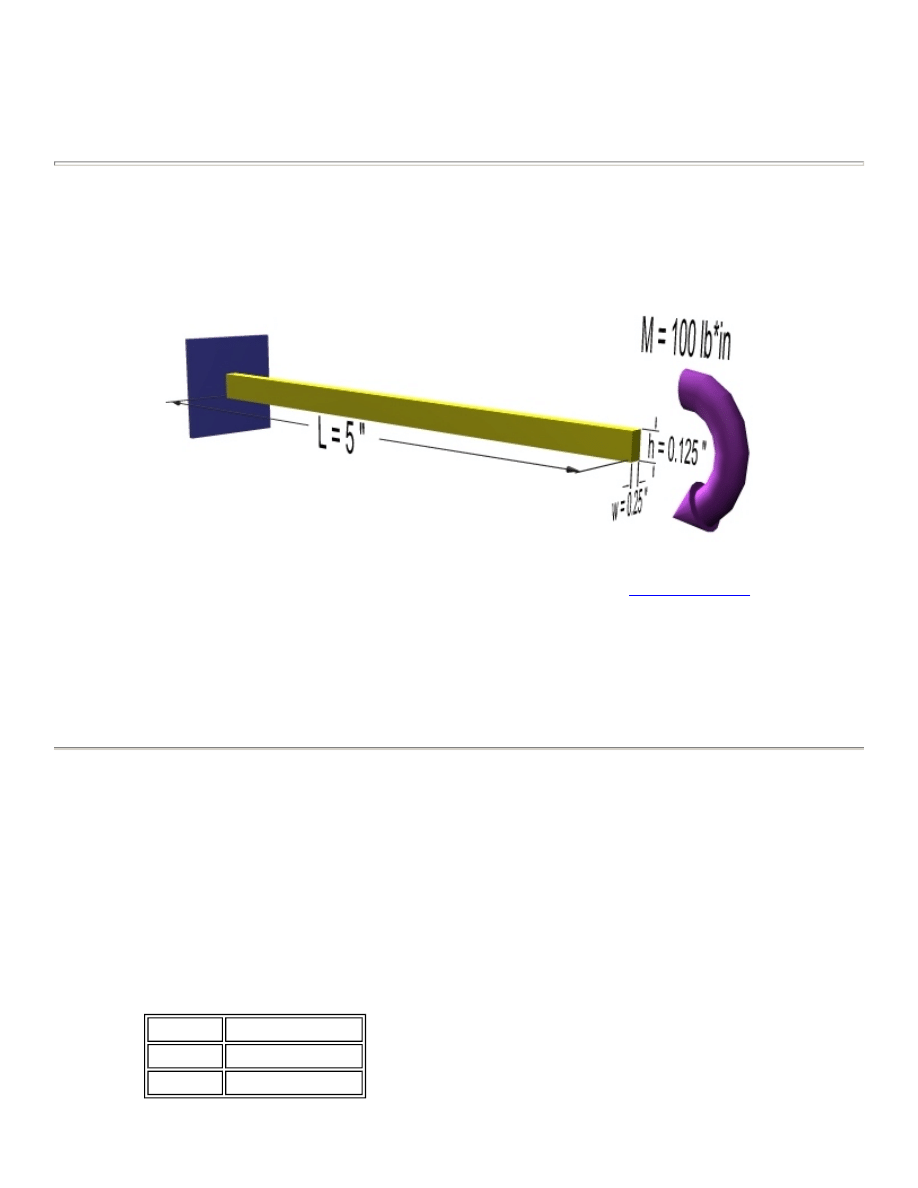
This tutorial was created using ANSYS 7.0 The purpose of this tutorial is to outline the steps required to do a

simple nonlinear analysis of the beam shown below.

There are several causes for nonlinear behaviour such as Changing Status (ex.

contact elements

), Material

Nonlinearities and Geometric Nonlinearities (change in response due to large deformations). This tutorial will

deal specifically with Geometric Nonlinearities .

To solve this problem, the load will added incrementally. After each increment, the stiffness matrix will be
adjusted before increasing the load.

The solution will be compared to the equivalent solution using a linear response.

Preprocessing: Defining the Problem

1. Give example a Title

Utility Menu > File > Change Title ...

2. Create Keypoints

Preprocessor > Modeling > Create > Keypoints > In Active CS

We are going to define 2 keypoints (the beam vertices) for this structure to create a beam with a

length of 5 inches:

Keypoint Coordinates (x,y)

(0,0)

(5,0)

University of Alberta ANSYS Tutorials - www.mece.ualberta.ca/tutorials/ansys/IT/NonLinear/NonLinear.ht...

3. Define Lines

Preprocessor > Modeling > Create > Lines > Lines > Straight Line

Create a line between Keypoint 1 and Keypoint 2.

4. Define Element Types

Preprocessor > Element Type > Add/Edit/Delete...

For this problem we will use the BEAM3 (Beam 2D elastic) element. This element has 3 degrees of
freedom (translation along the X and Y axis's, and rotation about the Z axis). With only 3 degrees
of freedom, the BEAM3 element can only be used in 2D analysis.

5. Define Real Constants

Preprocessor > Real Constants... > Add...

In the 'Real Constants for BEAM3' window, enter the following geometric properties:

i. Cross-sectional area AREA: 0.03125

ii. Area Moment of Inertia IZZ: 4.069e-5

iii. Total beam height HEIGHT: 0.125

This defines an element with a solid rectangular cross section 0.25 x 0.125 inches.

6. Define Element Material Properties

Preprocessor > Material Props > Material Models > Structural > Linear > Elastic > Isotropic

In the window that appears, enter the following geometric properties for steel:

i. Young's modulus EX: 30e6

ii. Poisson's Ratio PRXY: 0.3

If you are wondering why a 'Linear' model was chosen when this is a non-linear example, it is

because this example is for non-linear geometry, not non-linear material properties. If we were
considering a block of wood, for example, we would have to consider non-linear material
properties.

7. Define Mesh Size

Preprocessor > Meshing > Size Cntrls > ManualSize > Lines > All Lines...

For this example we will specify an element edge length of 0.1 " (50 element divisions along the
line).

8. Mesh the frame

Preprocessor > Meshing > Mesh > Lines > click 'Pick All'

LMESH,ALL

Solution: Assigning Loads and Solving

1. Define Analysis Type

University of Alberta ANSYS Tutorials - www.mece.ualberta.ca/tutorials/ansys/IT/NonLinear/NonLinear.ht...

Solution > New Analysis > Static

ANTYPE,0

2. Set Solution Controls

{

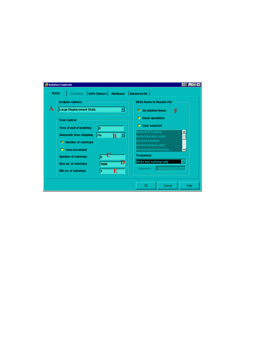
Select Solution > Analysis Type > Sol'n Control...

The following image will appear:

Ensure the following selections are made (as shown above)

A. Ensure Large Static Displacements are permitted (this will include the effects of large

deflection in the results)

B. Ensure Automatic time stepping is on. Automatic time stepping allows ANSYS to determine

appropriate sizes to break the load steps into. Decreasing the step size usually ensures better

accuracy, however, this takes time. The Automatic Time Step feature will determine an
appropriate balance. This feature also activates the ANSYS bisection feature which will

allow recovery if convergence fails.

C. Enter 5 as the number of substeps. This will set the initial substep to 1/5

of the total load.

The following example explains this: Assume that the applied load is 100 lb*in. If the
Automatic Time Stepping was off, there would be 5 load steps (each increasing by 1/5

the total load):

20 lb*in

40 lb*in

60 lb*in

80 lb*in

University of Alberta ANSYS Tutorials - www.mece.ualberta.ca/tutorials/ansys/IT/NonLinear/NonLinear.ht...

100 lb*in

Now, with the Automatic Time Stepping is on, the first step size will still be 20 lb*in.
However, the remaining substeps will be determined based on the response of the material

due to the previous load increment.

D. Enter a maximum number of substeps of 1000. This stops the program if the solution does

not converge after 1000 steps.

E. Enter a minimum number of substeps of 1.

F. Ensure all solution items are writen to a results file.

NOTE

There are several options which have not been changed from their default values. For more

information about these commands, type

help

followed by the command into the command line.

3. Apply Constraints

Solution > Define Loads > Apply > Structural > Displacement > On Keypoints

Fix Keypoint 1 (ie all DOFs constrained).

4. Apply Loads

Function

Command Comments

Load Step

KBC

Loads are either linearly interpolated (ramped) from the one
substep to another (ie - the load will increase from 10 lbs to 20 lbs

in a linear fashion) or they are step functions (ie. the load steps
directly from 10 lbs to 20 lbs). By default, the load is ramped. You

may wish to use the stepped loading for rate-dependent behaviour
or transient load steps.

Output

OUTRES This command controls the solution data written to the database.

By default, all of the solution items are written at the end of each
load step. You may select only a specific iten (ie Nodal DOF

solution) to decrease processing time.

Stress

Stiffness

SSTIF

This command activates stress stiffness effects in nonlinear

analyses. When large static deformations are permitted (as they are
in this case), stress stiffening is automatically included. For some

special nonlinear cases, this can cause divergence because some
elements do not provide a complete consistent tangent.

Newton
Raphson

NROPT

By default, the program will automatically choose the Newton-
Raphson options. Options include the full Newton-Raphson, the
modified Newton-Raphson, the previously computed matrix, and

the full Newton-Raphson with unsymmetric matrices of elements.

Convergence

Values

CNVTOL By default, the program checks the out-of-balance load for any

active DOF.

University of Alberta ANSYS Tutorials - www.mece.ualberta.ca/tutorials/ansys/IT/NonLinear/NonLinear.ht...

Solution > Define Loads > Apply > Structural > Force/Moment > On Keypoints

Place a -100 lb*in moment in the MZ direction at the right end of the beam (Keypoint 2)

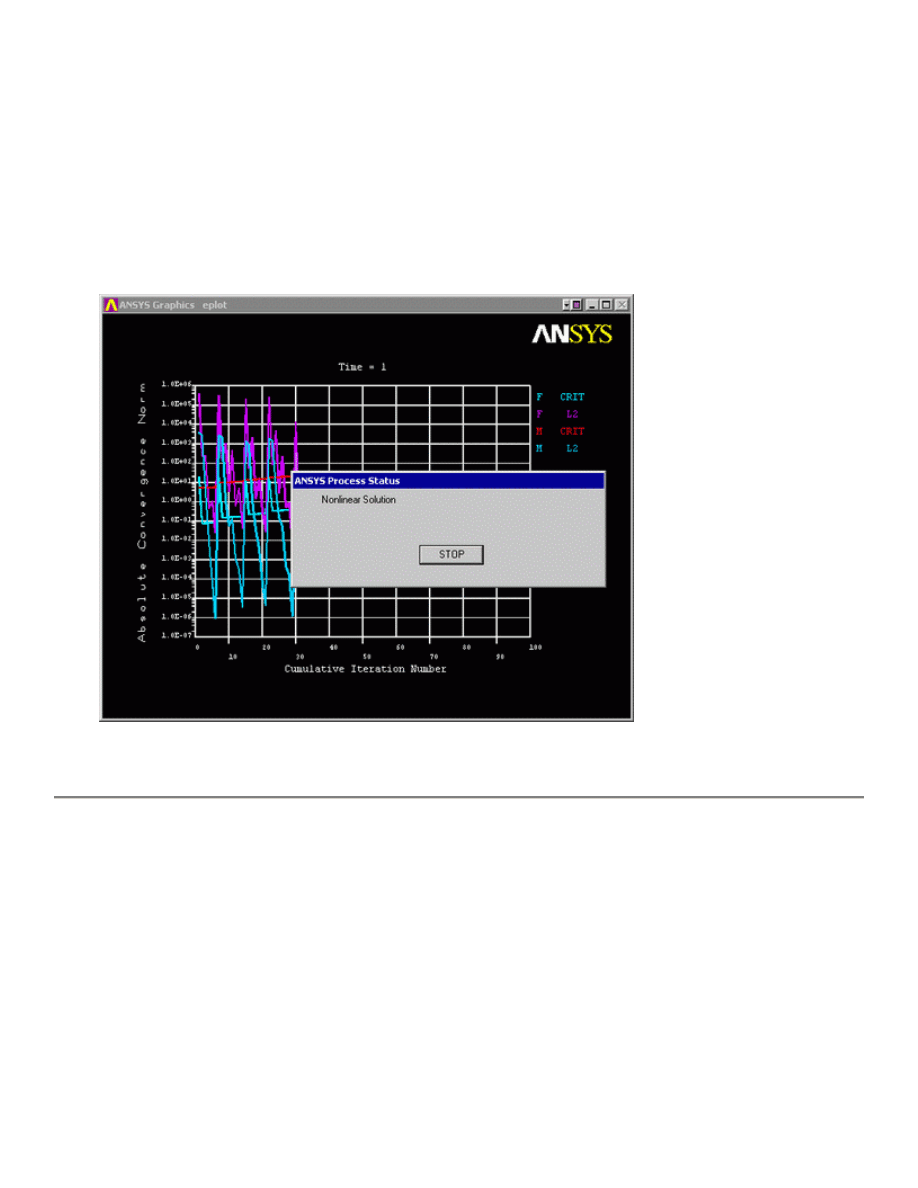
5. Solve the System

Solution > Solve > Current LS

SOLVE

The following will appear on your screan for NonLinear Analyses

This shows the convergence of the solution.

General Postprocessing: Viewing the Results

1. View the deformed shape

General Postproc > Plot Results > Deformed Shape... > Def + undeformed

PLDISP,1

University of Alberta ANSYS Tutorials - www.mece.ualberta.ca/tutorials/ansys/IT/NonLinear/NonLinear.ht...

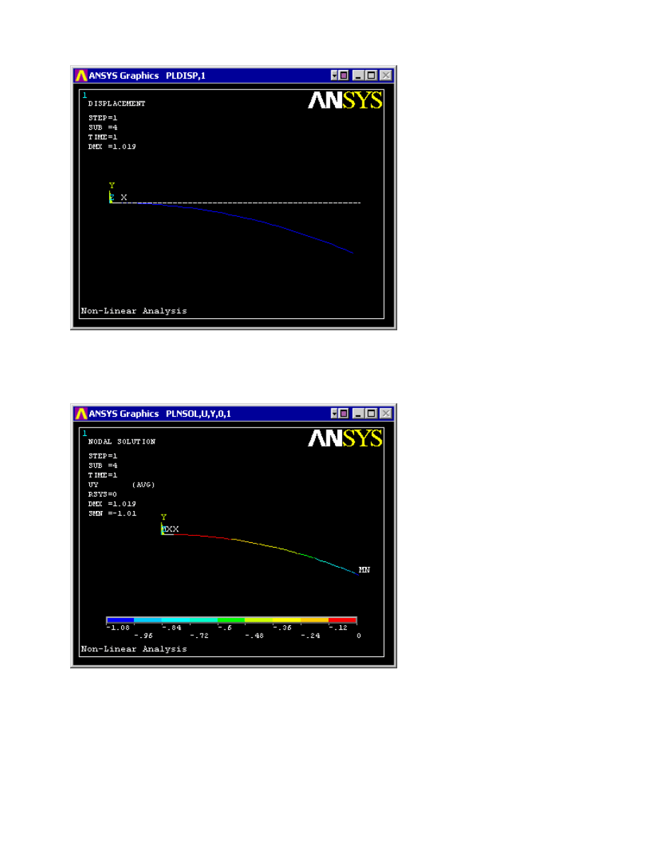
2. View the deflection contour plot

General Postproc > Plot Results > Contour Plot > Nodal Solu... > DOF solution, UY

PLNSOL,U,Y,0,1

3. List Horizontal Displacement

If this example is performed as a linear model there will be no nodal deflection in the horizontal

direction due to the small deflections assumptions. However, this is not realistic for large
deflections. Modeling the system non-linearly, these horizontal deflections are calculated by

ANSYS.
General Postproc > List Results > Nodal Solution...> DOF solution, UX

University of Alberta ANSYS Tutorials - www.mece.ualberta.ca/tutorials/ansys/IT/NonLinear/NonLinear.ht...

Other results can be obtained as shown in previous linear static analyses.

Command File Mode of Solution

The above example was solved using a mixture of the Graphical User Interface (or GUI) and the

command language interface of ANSYS. This problem has also been solved using the

ANSYS command

language interface

that you may want to browse. Open the file and save it to your computer. Now go to

'File > Read input from...' and select the file.

University of Alberta ANSYS Tutorials - www.mece.ualberta.ca/tutorials/ansys/IT/NonLinear/NonLinear.ht...