On the Semantics of Self-Unpacking Malware Code

∗

Saumya K. Debray

Kevin P. Coogan

Gregg M. Townsend

Department of Computer Science,

University of Arizona, Tucson, AZ 85721, USA.

{

debray, kpcoogan, gmt

}

@cs.arizona.edu

Abstract

The rapid increase in attacks on software systems

via malware such as viruses, worms, trojans, etc., has
made it imperative to develop effective techniques for
detecting and analyzing malware binaries.

Such bi-

naries are usually transmitted in packed or encrypted
form, with the executable payload decrypted dynami-
cally and then executed. In order to reason formally
about their execution behavior, therefore, we need se-
mantic descriptions that can capture this self-modifying
aspect of their code. However, current approaches to
the semantics of programs usually assume that the pro-
gram code is immutable, which makes them inapplicable
to self-unpacking malware code. This paper takes a step
towards addressing this problem by describing a formal
semantics for self-modifying code. We use our seman-
tics to show how the execution of self-unpacking code
can be divided naturally into a sequence of phases, and
uses this to show how the behavior of a program can be
characterized statically in terms of a program evolution
graph. We discuss several applications of our work, in-
cluding static unpacking and deobfuscation of encrypted
malware and static cross-phase code analysis.

1

Motivation

The rapid increase in the use of the Internet in many

aspects of our lives has led to an explosive growth in
the spread of malware such as computer worms, viruses,
trojans, spyware, and bots. Software security consid-
erations have accordingly become a crucial aspect of
modern software design, development, and deployment.
Since software—both new applications to be installed
on a system and patches or upgrades to existing ones—is

∗

This work was supported in part by the National Science Founda-

tion via grant nos. CNS-0410918 and CNS-0615347, and by the Air
Force Office of Scientific Research via grant no. FA9550-07-1-0019.

commonly distributed in the form of binaries, the ability
to verify that a binary file received from elsewhere does
not have any malicious content is an important com-
ponent of software security (for example, email attach-
ments are now routinely subjected to virus scans).

Most malware executables today are transmitted in

“scrambled” form. There are two commonly used ap-
proaches to such code scrambling: encryption and pack-
ing. The former refers to the use of some kind of in-
vertible operation, together with an encryption key, to
conceal the executable code; the latter refers to the use
of compression techniques to reduce the size of the mal-
ware payload while at the same time converting it to a
form where the executable content is hidden. In either
case, the scrambled code is “unpacked” at runtime prior
to execution; in many cases, there are multiple rounds of
unpacking during the course of an execution.

1

Such self-

unpacking malware code is, therefore, self-modifying.

In order to build effective defences against malware,

we have to be able to obtain a precise understand their
behavior. This makes it important to be able to reason
formally about the code and the behavior(s) of malware.
Such reasoning can be helped greatly by a formal se-
mantics that is able, among other things, to cope with
self-modifying code. Unfortunately, current approaches
to program semantics typically assume that the program
code is immutable, which makes them unsuitable for
this purpose. This poses a problem, which this paper at-
tempts to address. We motivate our approach using the
example application of static analysis of self-unpacking
malware code.

The usual approach to dealing with packed binaries—

especially when analyzing malware that has not been

1

For most of the paper, we will not be greatly concerned by the

technical distinction between the operations of encryption and packing
(for changing a program to its scrambled form) on the one hand, and
between decryption and unpacking (for the reverse operation) on the
other. In order to simplify the presentation, therefore, we will generi-
cally use the term packing to refer to the former and unpacking to refer
to the latter.

1

0

P

∆

1

∆

3

3

P

∆

2

1

P

2

P

∆

i

i

P

: code change mechanisms

: code snapshots

Figure 1. An example of a behavioral model for a self-modifying program

previously encountered—is to use dynamic analysis
techniques, e.g., by running the binary in an emulator
or under the control of a debugger. However, dynamic
analysis can be tedious and time-consuming, and can
be defeated via anti-monitoring and anti-virtualization
techniques that allow the malware to detect when its
code is being run under the control of a debugger or
emulator [4, 6, 14, 19]. Furthermore, even if the un-
packer code is activated during a dynamic analysis, the
code may be unpacked over many rounds of unpacking
in such a way that the amount of code that is materialized
on any given round is small enough to escape detection,
thereby leading to false negatives.

These shortcomings of dynamic malware analysis

lead us to revisit the question of static analysis of mal-
ware binaries. However, this faces the hurdle that since
self-unpacking malware effectively change their code
on the fly, existing semantic bases for static analysis—
which typically assume a fixed program—are inade-
quate for reasoning about them. We need a semantic
framework that is able to capture the dynamic genera-
tion and modification of a program’s code during execu-
tion. Furthermore, while most of the proposals for dy-
namic code modification in the research literature, e.g.,
in the context of just-in-time compilation [1] or dynamic
code optimization [3, 16, 18], tend to modify code in
principled ways, the code for dynamic malware unpack-
ing tends to be sneaky and obscure, often using arbi-
trary arithmetic operations on memory such as addition,
XOR, rotation, etc., to effect the code changes needed.
This makes the development of a formal semantics for
such programs a nontrivial challenge.

This paper makes two contributions in this regard.

First, it takes a step in addressing this challenge by
proposing a formal semantics for a simple “abstract as-
sembly language” that permits dynamic code modifica-
tion. Second, it shows a number of example applica-

tions for this semantic framework, including (1) static
unpacking and analysis of packed malware binaries; (2)
generalizing the traditional notions of “liveness” and
“dead code” to self-modifying code, and applying this
to malware deobfuscation; and (3) static identification of
dynamic anti-monitoring defenses. Our ideas are not in-
tended to replace the dynamic analyses currently used by
security researchers, but to complement them and pro-
vide researchers with an additional tool for understand-
ing malware.

2

Behavioral Models

Static analyses generally construct behavioral mod-

els for programs, i.e., static program representations that
can be used to reason about its runtime behavior; exam-
ples include graph-based representations, such as con-
trol flow graphs and program dependence graphs, com-
monly used by compilers. Typically, such behavioral
models contain program code (e.g., basic blocks) as well
as control or data flow relationships between them that
can be used to obtain insights into the execution behav-
ior of the program.

Traditional program analyses typically assume that

the program does not change during the course of ex-
ecution. This assumption generally holds for ordinary
application code, so it suffices to use a simple behavioral
model that contains a single “snapshot” of a program’s
code. This assumption does not hold for malware, how-
ever, since malware code very often changes as exe-
cution progresses. For example, the Rustock rootkit
and spambot arrives as a small unpacking routine to-
gether with an encrypted payload. When executed, this
code unpacks the code for a rootkit loader, which subse-
quently carries out a second round of unpacking to gen-
erate the code for the rootkit itself [7]. This program,

2

therefore, requires three different code snapshots to de-
scribe its behavior.

Since our goal is to reason statically about malware

code, it becomes necessary for us to develop more gen-
eral behavioral models that can cope with changes to the
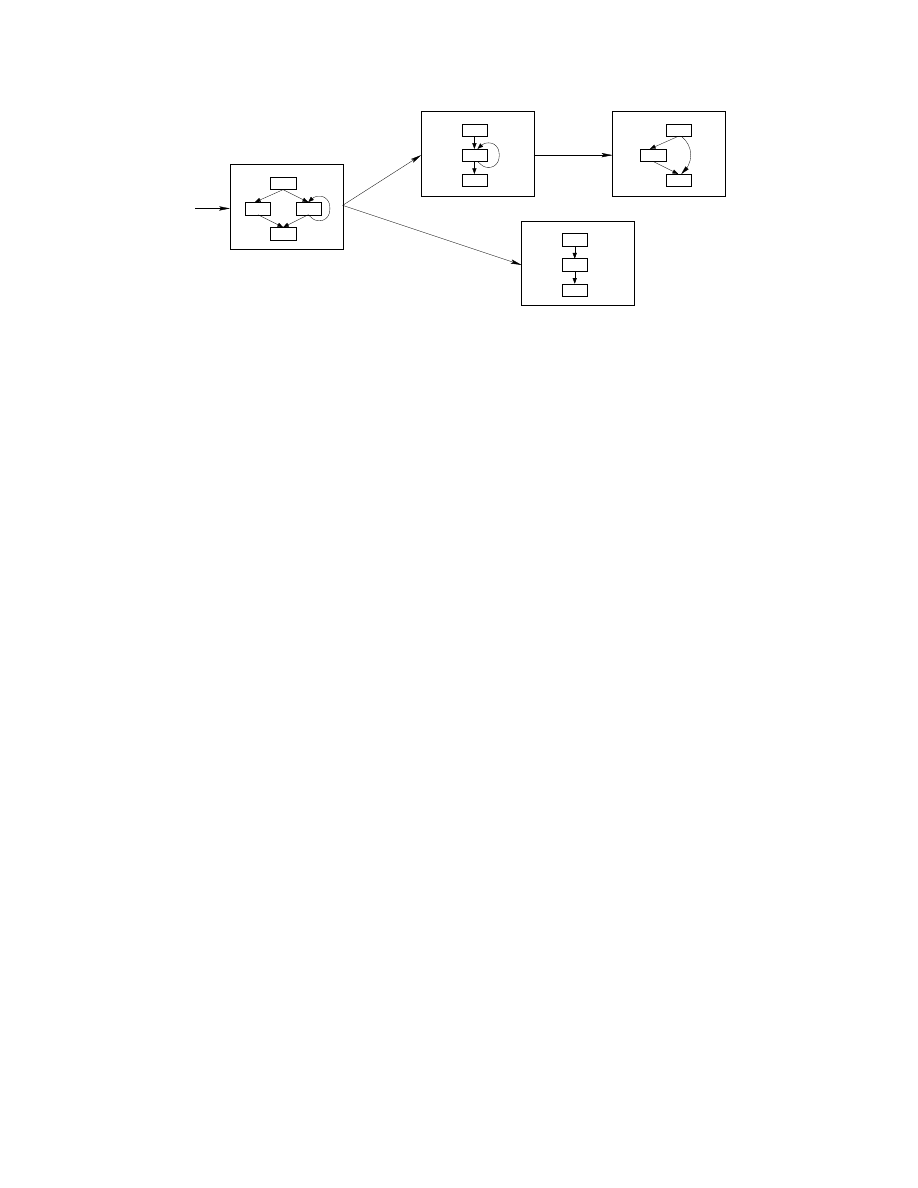
program code at runtime. Figure 1 shows an example
this. It is a directed graph where each vertex P

i

is a tra-

ditional static program representation and whose edges
represent possible runtime changes: an edge P

i

→ P

j

indicates that the code P

i

may change to the code P

j

at runtime. Furthermore, each edge has a label

∆

i

that

represents the mechanism for the corresponding code
change. For example, each vertex may be a control flow
graph for a code snapshot encountered at runtime while
the label on each edge is a program slice that effects the
corresponding code change. This allows us to reason
about both the code snapshots P

i

as they exist in be-

tween changes to the code, as well as the mechanisms
∆

i

used to effect those changes. Sections 3 and 4 dis-

cuss a semantic formulation for machine-level programs
that forms the underpinning of such reasoning; Section
5 then discusses the details of how such a behavioral
model may be constructed.

3

An Abstract Assembly Language

In order to define and prove the correctness of static

analyses for malware, we need to specify the language
semantics underlying the analysis. This turns out to
be problematic for malware because malware code is
typically self-modifying, while most language seman-
tics considered in the literature assume that the program
code is immutable. We therefore begin by describing
the syntax and semantics for a small, low-level abstract
assembly language that allows dynamic code modifica-
tion.

3.1

Syntax

Figure 2 gives the syntax of our abstract assembly

language. For the sake of generality, we abstract away
architecture-specific details, e.g., as the distinction be-
tween registers and memory, various addressing modes,
etc. We assume an infinite set of memory locations in-
dexed by the natural numbers

N

. Operations include

assignment, input, and conditional and unconditional
branches, the last of which include both direct and in-
direct branches. The set of instructions is denoted by

I

.

Computations are over the set of natural numbers

N

.

Malware code is typically encountered in the form of

executable binaries. We model this using the notion of

Syntactic Categories:

a, n

∈

N

(integers)

e

∈

E

(expressions)

I

∈

I

(instructions)

M

∈

M =

N

−→

N

⊥

(memory map)

P

∈

M ×

N

(programs)

Syntax:

e

::=

n

(constant)

|

MEM

[e

1

]

(contents of memory)

|

e

1

op e

2

(arithmetic)

op

∈ {+, −, . . .}

I

::=

MEM

[e

1

] := e

2

(assignment)

|

input

⇒

MEM

[e

1

]

(input)

|

if

e

1

goto

a

(conditional branch)

|

goto

e

(unconditional branch)

|

halt

Figure 2. An abstract assembly language:
Syntax

memory maps: A memory map M

∈

M

=

N

−→

N

⊥

and denotes the contents of a program’s memory (loca-
tions that do not have a defined value are assumed to be
implicitly mapped to

⊥).

An important aspect of low-level program represen-

tations on real processors is that there is no fundamental
distinction between code and data: memory locations
contain binary values that can be interpreted either as
representing data or as encoding program instructions.
This makes it possible to operate on a memory location
as though it contains data, e.g., by adding or subtract-
ing some value from it, and then interpret the result as
code and execute it. To capture this, we assume the ex-
istence of an injective function encode

:

I

−→

N

such

that, given I

∈

I

, the value encode

(I) ∈

N

gives its

binary representation. We have a corresponding notion
of “decoding” a number to the instruction it represents,
denoted by a function decode, which extends encode

−1

to a total function by mapping numbers that do not cor-
respond to legal instruction encodings to

⊥:

decode

(n) :

N

−→ I

⊥

decode

(n) =

I

if

∃I ∈

I

s.t. encode

(I) = n

⊥ otherwise

Syntactically, a program P

∈ M×

N

consists of a mem-

ory map together with the entry point, i.e., the address
where execution begins. Given a program P

= (M, a),

the memory map M specifies the contents of all of P ’s
memory, including both code and data.

To simplify the discussion, we assume that each in-

struction occupies a single location in memory. While

3

this does not hold true of variable-instruction-length ar-
chitectures such as the Intel IA-32, the issues raised by
variable-length instructions are orthogonal to the topic
of this paper.

3.2

Semantics

The semantics of this language are given in Figure

3. We use the following notation. The set S

⊥

denotes

S

∪{⊥}. The Kleene closure of a set S, i.e., the set of all

finite sequences of elements of S, is written S

∗

. Given

a function f

: A → B, f [a 7→ b] denotes the function

λx.

[if x = a then b else f (x)], which is the same as f

except at a, where its value is b.

A store σ

∈ M is simply a memory map, and maps

locations to values. A program state

(a, σ, θ) has three

components: a is the “program counter value,” which
is either

⊥ (indicating an undefined location), or 8 (in-

dicating that the program is halted), or else is an inte-
ger giving the location of the next instruction to exe-
cute; σ

∈ M is the store and represents the contents of

memory; and θ

∈ Θ represents the unexpended input

in the input stream. The equations defining the func-
tion E , which specifies the meaning of expressions, are
straightforward. The definition of I , the semantic func-
tion describing the behavior of instructions, shows the
low-level nature of the language: I takes a state as ar-
gument, uses the value of the program counter compo-
nent a of its argument to retrieve the contents σ

(a) of

the corresponding memory location, decodes this value
using the decoding function decode, then executes the
resulting instruction. The program counter value after
the execution of an instruction at location a depends on
the type of instruction: for control transfer instructions,
the next program counter is specified as a target of the
instruction itself; otherwise, the program counter value
is that of the next instruction, at location a

+ 1.

Four of the five instructions in our language—

assignment,

conditional

branches,

unconditional

branches, and

halt

—are familiar and have the expected

semantics, as shown in Figure 3. The fifth instruction,
‘input

⇒

MEM

[e]’, is used to read in external input.

The idea here is that the next value in the input stream
is written to the memory location with address e. We
use the notion of “external input” to refer to any source
that is external to the program: it may refer to a human
user, another program executing on the same computer,
input that is read in from the program’s execution
environment or over a network from a remote host, etc.
(We note in passing that the language shown does not
have instructions for procedure calls and returns. This
omission is primarily to keep the discussion simple:

it would be straightforward to extend our language to
deal with procedure calls by adding

call

and

return

instructions to the instruction set together with an
additional stack component to each state.)

Define the predicate hasSucc on states such that

hasSucc

(t) is true if and only if the state t has a suc-

cessor, i.e., it is not undefined and not a halted state:

hasSucc

(t)

△

= t 6= ⊥ and ∀σ, θ : t 6= (8, σ, θ).

Given a program P

= (M, a

0

) and an input stream θ, its

initial state is given by σ

0

[P, θ] = (M, a

0

, θ

). Given this

initial state, and the transition relation I

: Σ −→ Σ,

we can now specify a trace semantics for a program as
follows. First, define the set of finite traces of a program
P for an input stream θ to be

T JP, θK = {t0 . . . t

k

| t

0

= σ

0

[P, θ] and

(∀i : 0 ≤ i < k)[hasSucc(t

i

) and

t

i+1

= I Jt

i

K]}.

The set of all finite traces of a program P is then given

by T

JP K =

[

θ∈Θ

T JP, θK.

3.3

Reachability

The notion of reachability will be important in the

discussion that follows. Intuitively, a location ℓ

1

is stat-

ically reachable from a location ℓ

0

if, under the usual

static analysis assumption that either branch of a condi-
tional may be taken at runtime, it is possible for control
to go from the instruction at location ℓ

0

to the instruc-

tion at location ℓ

1

. The reason we refer to it as “static

reachability” is that it assumes that the program code is
static, i.e., is not being modified during execution. We
first define the notion of a control-flow successor:

Definition 3.1 Let P

= (σ, a) be a program and I =

decode

(σ(ℓ

0

)) the instruction in P at location ℓ

0

. The

location ℓ

1

is a control-flow successor of ℓ

0

in P (written

‘ℓ

0

;

P

ℓ

1

’) if one of the following hold:

– I

= p

MEM

[e

1

] := e

2

q and ℓ

1

= ℓ

0

+ 1;

– I

= pinput ⇒

MEM

[e

1

]q and ℓ

1

= ℓ

0

+ 1;

– I

= p

if

e

1

goto

a

1

q and ℓ

1

∈ {a

1

, ℓ

0

+ 1};

– I

= p

goto

e

1

q and ℓ

1

= E Je

1

K σ.

4

Value Domains:

σ

∈ M

=

N

−→

N

⊥

(store)

θ

∈ Θ

=

N

∗

(input stream)

π

=

N

∪ {⊥, 8}

(program counter values)

Σ

=

π

× M × Θ

(program states)

Semantics:

E

XPRESSIONS

:

E

:

E

× M −→

N

⊥

E

JnK σ

=

n

E

J

MEM

[e]K σ

=

let n

= E JeK σ in

if n

6= ⊥ then σ(n)

else

⊥

E

Je

1

op e

2

K σ

=

let n

1

= E Je

1

K σ n

2

= E Je

2

K σ in

if n

1

6= ⊥ and n

2

6= ⊥ then n

1

op n

2

else

⊥

I

NSTRUCTIONS

: The semantic function I

: Σ → Σ gives the effect of executing an instruction.

It

effectively specifies the transition relation between states.

I

(JaK , σ, θ) = case decode(σ(a)) of

p

MEM

[e

1

] := e

2

q

:

let n

1

= E Je

1

K σ, n

2

= E Je

2

K σ in

if n

1

6= ⊥ and n

2

6= ⊥ then (a + 1, σ[n

1

7→ n

2

], θ); else ⊥

pinput ⇒

MEM

[e

1

]q

:

let n

1

= E Je

1

K σ in

if n

1

6= ⊥ and length(θ) > 0 then (a + 1, σ[n

1

7→ hd (θ)], tl (θ)); else ⊥

p

if

e

1

goto

a

1

q

:

let n

1

= E Je

1

K σ in

if n

1

6= ⊥ then

if n

1

6= 0 then (a

1

, σ, θ

); else (a + 1, σ, θ)

else

⊥

p

goto

e

1

q

:

let n

1

= E Je

1

K σ in

if n

1

6= ⊥ then (n

1

, σ, θ

); else ⊥

p

halt

q

:

(8, σ, θ)

⊥

:

⊥

Figure 3. An abstract assembly language: Semantics

The first two cases above correspond to execution fall-
through in non-control-transfer instructions, while the
remaining two cases refer to the behavior of control
transfers. The notion of static reachability is simply the
reflexive transitive closure of the control-flow successor
relation:

Definition 3.2 A location ℓ

1

is statically reachable

from a location ℓ

0

in a program P , denoted by ℓ

0

;

∗
P

ℓ

1

, if:

(i) ℓ

0

= ℓ

1

; or

(ii) there exists a location ℓ such

that ℓ

0

;

P

ℓ and ℓ ;

∗
P

ℓ

1

.

4

Giving Structure to Dynamic Code
Modification

Before we can discuss dynamically modified code,

we must specify exactly what that term means.

We

interpret this narrowly. It is not enough for the pro-

gram to simply modify some memory regions that typi-
cally contain code,

2

such as the .text section, since pro-

grams sometimes contain data embedded in the instruc-
tion stream. On the other hand, we want to be able
to catch programs that dynamically generate and exe-
cute code in memory regions that usually do not contain
code, e.g., the stack or heap. We require, therefore, that a
memory location must be modified (i.e., written to) and
subsequently executed:

Definition 4.1 A trace T

= t

0

. . . t

i

. . . t

j

. . . is code-

modifying if and only if it contains states t

i

and t

j

,

j > i, such that t

i

modifies a memory location a and

t

j

executes the instruction at location a.

A program P is code-modifying if and only if there

is some trace T

∈ T JP K that is code-modifying.

2

Some researchers have used this criterion as a heuristic to identify

self-modifying code [17].

5

A particular execution of a program can modify its

code numerous times [7]. Given an execution trace T
for a program P , it is conceptually convenient to distin-
guish between the code that is changing memory loca-
tions that may be executed at some future point from the
code that is encountered when one of those modified lo-
cations is eventually executed. We do this by dividing
up an execution trace into phases:

Definition 4.2 A phase T

′

of a trace T is a maximal

subsequence of T such that T

′

does not execute any lo-

cation modified by T

′

.

This means that all phases but the first always begin with
the execution of an instruction that was created and/or
modified in a previous phase.

The following result captures a crucial property of

phases: namely, that for each state S

i

in the phase, the

contents of memory at the program counter location a

i

for that state is the same as the contents of location a

i

at

the beginning of that phase.

Theorem 4.1 Let φ

= S

0

, . . . , S

i

, . . . be a phase, with

S

i

= (a

i

, M

i

, θ

i

), then M

i

(a

i

) = M

0

(a

i

) for all S

i

∈

φ.

Proof By contradiction. Suppose that the proposition
does not hold, i.e., M

i

(a

i

) 6= M

0

(a

i

) for some state

S

i

∈ φ. Then it must be the case that memory location

a

i

is modified by some earlier state S

j

∈ φ, j < i.

Thus, S

i

∈ φ executes a location modified by S

j

∈ φ.

From the definition of a phase, this means that S

i

and

S

j

cannot be in the same phase. Thus, either S

i

6∈ φ or

S

j

6∈ φ, which is a contradiction. The theorem follows.

This theorem implies that for each state S

i

in a phase,

the instruction “seen” at location a

i

by S

i

, when control

reaches a

i

, is the same as the instruction at that location

at the beginning of the phase:

Corollary 4.2 Let φ

= S

0

, . . . , S

i

, . . . be a phase for a

program, with S

i

= (a

i

, M

i

, θ

i

). Then for all S

i

∈ φ,

the instruction at location a

i

that is executed in state S

i

is the same as the instruction occurring at location a

i

in

the initial state S

0

of φ.

This corollary means that the static code “snapshot”

at the beginning of a phase gives the program that is ex-
ecuted by that phase, and can be used as a basis for ana-
lyzing and understanding the behavior of that phase.

We next consider the question of partitioning a trace

into phases. Intuitively, given a trace of a program’s ex-
ecution, we can simply replay the trace keeping track

of memory locations that are modified due to the ex-
ecution of each instruction, and thereby identify those
states where the instruction about to be executed is at a
location that was modified in the current phase. Each
such state then marks the beginning of a new phase.
More formally, the process of partitioning a trace into
phases can be described as follows. For any instruction
I, let

MOD

JIK σ denote the set of locations modified by

I given a store σ:

MOD

JIK σ =



































{n

1

} if I = p

MEM

[e

1

] := e

2

q

and n

1

= E Je

1

K σ

{n

1

} if I = pinput ⇒

MEM

[e

1

]q

and n

1

= E Je

1

K σ

∅

otherwise

Given a trace T

= t

0

t

1

. . . t

n

, let t

i

= (a

i

, σ

i

, θ

i

), let the

instruction at location a

i

, which is about to be executed,

be I

i

= decode(σ(a

i

)). We first define functions ∆

−

and

∆

+

that give the set of memory side effects of the

current phase:

∆

−

(t) gives the set of locations written

to upto state t, i.e., at the point where the instruction I
specified by t’s program counter is about to be executed,
while

∆

+

(t) gives this set after I has executed. For any

state t

= (a, σ, θ), let I = decode(σ(a)) be the instruc-

tion executed in t, then the value of

∆

+

(t) is defined as

follows:

∆

+

(t) = ∆

−

(t) ∪

MOD

JIK σ

The function

∆

−

is defined as follows. For the very

first state t

0

of the trace, no code has been executed

and therefore no memory modifications have occurred.
For a later state t

i+1

, the value of

∆

−

(t

i+1

) depends

on whether t

i+1

is the first state in a new phase. If the

program counter a

i+1

in this state is an address that has

been modified in

∆

+

(t

i

), then t

i+1

starts a new phase,

and since no instructions in this new phase have been
executed, the memory effects of the phase are empty.
Otherwise, t

i+1

simply extends the current phase, so

∆

−

(t

i+1

) = ∆

+

(t

i

). Thus, we have:

∆

−

(t

0

)

=

∅

∆

−

(t

i+1

) =







∅

if a

i+1

∈ ∆

+

(t

i

)

∆

+

(t

i

)

otherwise

We can now specify how to partition a trace T into a
sequence of phases. Given a state t

∈ T , let φ(t) ∈

N

be

its phase number, which denotes which phase it belongs
to. We can use the

∆

+

function to assign phase numbers

to states:

6

φ

(t

0

) = 0

φ

(t

i+1

) =

φ

(t

i

) + 1

if a

i+1

∈ ∆

+

(t

i

)

φ

(t

i

)

otherwise

Then, each phase φ

i

is a maximal subsequence of T such

that all of the states in φ

i

have the same phase number.

Recall that, as mentioned in Section 2, one of our

goals is to construct static behavioral models for pro-
grams with dynamically modified code, which capture
both “code snapshots” as well as code change mecha-
nisms, i.e., the code that is responsible for dynamically
modifying the code. In preparation for this, we first out-
line how we can abstract away from the trace seman-
tics of a program to a description that records only the
possible code snapshots and code change mechanisms
that occur over all possible executions of the program.
First, given a phase φ

= t

0

, . . . , t

n

in a trace T , where

t

i

= (a

i

, σ

i

, θ

i

), 0 ≤ i ≤ n, we specify two characteris-

tics of φ:

– The code snapshot for the phase, denoted by

code

(φ). From Theorem 4.1, this is given by the

program at the first state of the phase:

code

(φ) = (σ

0

, a

0

).

– The code responsible for changes to memory that

occur during the execution of φ, denoted by
dmods

(φ). Since the set of memory locations mod-

ified during the execution of φ is given by

∆

+

(t

n

),

this is given by the dynamic slice of code

(φ) for

the set of locations (i.e., variables)

∆

+

(t

n

) and the

history φ.

We can now define the dynamic evolution graph for a
program P to be an edge-labelled directed graph with
vertices V and edges E, given by the following:

– Let T

∈ T JP K be any execution trace for P , and

let φ be any phase of T . Then code

(φ) is a vertex

in V .

– Let T

∈ T JP K be any execution trace for P ; φ

i

and φ

i+1

be any two successive phases of T ; and

D

= dmods(φ

i

). Let v

i

and v

i+1

be vertices in V

corresponding to phases φ

i

and φ

i+1

respectively.

Then v

i

D

−→ v

i+1

is an edge in E.

The next section discusses how we can statically approx-
imate a program’s dynamic evolution graph to construct
a behavioral model which we call its “program evolution
graph.”

5

Program Evolution Graphs

This section discusses one concrete application of the

semantics described in the previous section. We show
how this semantics can be used as a formal basis for
constructing static behavioral models for self-modifying
programs, which can then be used to reason about the
behavior of such programs.

The dynamic evolution graph for a program P , dis-

cussed in the previous section, is an abstraction of its
trace semantics that describes some aspects of P ’s run-
time behavior. The program evolution graph for P is
a static approximation to P ’s dynamic evolution graph.
This section discusses the construction of such graphs.

Given an executable P , we initialize the program

evolution graph of G to contain P as its only vertex, then
proceed by iteratively analyzing the vertices. For each
vertex, our algorithm identifies transition edges that
specify control transfers into newly modified code (Sec-
tion 5.1), then processes each transition edge separately
to obtain (an approximation to) the code that would re-
sult from dynamic code modifications leading up to that
instruction (“static unpacking,” Section 5.2). The input
executable P has to contain the code for the initial un-
packer (which unpacker cannot itself be in packed form),
as well as a control flow path to this code so that it can
be executed; our algorithm begins by discovering tran-
sition edges out of this initial unpacker, then iteratively
processes the unpacked programs it identifies. The re-
sulting programs from static unpacking are then added
to the program evolution graph and eventually processed
in their turn. The discussion below focuses on the core
computations of of this nested iteration, namely, identi-
fication of transition points and the static unpacking for
any given transition point. The overall algorithm is sum-
marized in Figure 4.

5.1

Identifying Transition Edges

The first step of the analysis involves identifying

those instructions (equivalently, locations) in a program
that may mark a boundary between phases, i.e., from
which control may reach a location that has been modi-
fied by the current phase. We refer to such control flow
as a transition edge. For determining the locations that
may be modified during execution, we assume a binary-
level alias analysis that gives a superset of the set of pos-
sible referents of all (direct and indirect) memory refer-
ences. The issue of alias analysis—and, in particular,
binary-level alias analysis [12, 13]—is well-studied and
in any case orthogonal to the topic of this paper, and
we do not pursue the mechanics of such analyses further

7

Input: A program P

0

= (M

0

, a

0

).

Output: A program evolution graph G

= (V, E).

Method:

V

= {P

0

};

/* P

0

is unmarked */

E

= ∅;

while there are unmarked elements of V do

let P

= (σ, a) be any unmarked element of V ;

mark P ;
T

= TransitionEdges(P );

/* see Section 5.1 */

for each t

= (b, c) ∈ T do

/* static unpacking: see Section 5.2 */

M

:= Mods

P

(a, b);

/* locations modified on paths from a to b

S

:= backward static slice of P at b with respect to M ;

σ

′

:= store resulting from the symbolic execution of S;

P

′

:= (σ

′

, c

);

/* unpacked program */

if P

′

6∈ V then

add P

′

(unmarked) to V ; add ‘P

S

−

→ P

′

to E;

fi

od

/* for */

od

/* while */

return G;

Figure 4. Algorithm for static construction of program evolution graphs

here. We use the results of the alias analysis to identify
transition edges.

More formally, given a location ℓ and an instruction

I, let alias

I

(ℓ) denote (a superset of) the set of values

of memory location ℓ when control reaches I over all
possible executions of the program.

3

We generalize this

to val

I

(e), denoting the set of possible values taken on

by any expression e when control reaches I, by lifting
pointwise: the details are given in Figure 5. Then, for
each instruction I we compute two sets: write

(I), the

set of memory locations that may be written to by I;
and next

(I), the set of locations that control may go

to after the execution of I. The details of how these
functions are defined are given in Figure 5. Note that
next

(I) is in fact simply a static approximation to the

semantic relation ;

P

defined in Section 3.3. Transition

edges are then obtained as follows:

Definition 5.1 A transition edge for a program P is a
pair of locations

(a, b) such that the following hold:

3

In the context of more familiar source-level analyses, pointer alias

analyses compute, for each pointer, the set of objects it may point to.
At the assembly-code or machine-code level, this is equivalent to com-
puting, for each location that may be used as a pointer, the set of possi-
ble addresses—i.e., the values—contained at that location. In our case,
therefore, alias analysis amounts to computing the possible values at
each location in memory.

1. a

6∈ write(X) for any instruction X ∈ P ; and

2. let the instruction at location a be I

a

, then there

exists an instruction J in the program, at loca-
tion ℓ

J

, such that a is reachable from ℓ

J

and b

∈

write

(J) ∩ next(I

a

).

The definition states that while location a is not mod-
ified by the program (condition 1), location b may be
modified by J and control can then go from J to a and
thence to b (condition 2). Control enters the modified
code when it goes from a to b.

In general, a program may have multiple transition

edges, corresponding to different ways of modifying
a program.

Given a program P , we denote its set

of transition edges—which will, in general, be depen-
dent on the precision of the alias analysis used—by
TransitionEdges

(P ).

5.2

Static Unpacking

Once we have the set of transition edges for a pro-

gram P , we process them individually to determine, as
far as possible, the contents of memory after unpacking.

8

Given: an instruction I at location ℓ

I

.

val

I

(e) denotes the set of possible values of an expression e when control reaches I for all possible execu-

tions of the program:

val

I

(e) =











{n}

if e

= pnq

S{alias

I

(e

′

) | e

′

∈ val

I

(e

1

)}

if e

= p

MEM

[e

1

]q

{e

′
1

op e

′
2

| e

′
1

∈ val

I

(e

1

) and e

′
2

∈ val

I

(e

2

)}

if e

= pe

1

op e

2

q

write

(I) denotes the set of locations that may be modified by I over all possible executions of the program:

write

(I) =











val

I

(e

1

) if I = p

MEM

[e

1

] := e

2

q

val

I

(e

1

) if I = pinput ⇒

MEM

[e

1

]q

∅

otherwise

next

(I) denotes the set of locations that control may go to immediately after the execution of I:

next

(I) =



























{ℓ

I

+ 1}

if I

= p

MEM

[e

1

] := e

2

q

{ℓ

I

+ 1}

if I

= pinput ⇒

MEM

[e

1

]q

{a, ℓ

I

+ 1} if I = p

if

e

1

goto

aq

val

I

(e)

if I

= p

goto

eq

∅

if I

= phaltq

Figure 5. The functions

val

,

write

, and

next

(see Section 5.1)

We refer to this process as static unpacking. Of course,
given the usual undecidability problems that arise dur-
ing static analysis, this will not always be possible in
general, and our analysis will sometimes conservatively
indicate the contents of some memory locations to be
unknown.

Given a transition edge

(b, c) in a program P =

(σ, a), we first compute the set of locations Mods

P

(a, b)

that may be modified during the execution of P along
paths from a to b:

Mods

P

(a, b) =

[

I∈P

{write(I) | a ;

∗
P

I and I ;

∗
P

b

}.

Our next step is to isolate the fragment of P
whose execution may affect the values of locations in
Mods

P

(a, b). For this, we compute S, the backward

static slice of P for the set of locations (i.e., vari-
ables) Mods

P

(a, b).

The store resulting from these

modifications—which includes the modified code—is
then obtained by symbolic execution of S.

This symbolic execution of the slice S begins in the

memory state σ given by the initial store σ and proceeds
until it reaches the point where control would go from b

to c (recall that

(b, c) is the transition edge under consid-

eration). The details of exactly how the symbolic execu-
tion are carried out involve design and representation de-
cisions concerning, for example, tradeoffs between cost
and precision. For this reason, we do not pursue these
details here.

5.3

Putting it all Together

After static unpacking of each transition edge, we

update the program evolution graph. Given a program
P

= (σ, a) and a transition edge (b, c), let the memory

state resulting from static unpacking be σ

′

, then the re-

sult of static unpacking is the program P

′

= (σ

′

, c

). If

P

′

is new, we add it to the set of vertices of the program

evolution graph and the edge ‘P

S

−

→ P

′

’ to the set of its

edges.

Since one of the main reasons for constructing a pro-

gram evolution graph is for the analysis and understand-
ing of malware code, we may also want to disassemble
the program at each of its vertices and construct a con-
trol flow graph for it. Given a vertex P

= (σ, a), the

locations to be disassembled are given by

{ℓ | a ;

∗
P

ℓ

}.

9

The control flow graph for the resulting instruction se-
quence can be constructed in the usual way.

6

Applications

of

Program

Evolution

Graphs

This section sketches some applications of static

analysis of program evolution graphs for understanding
the behavior of malware binaries.

6.1

Exec-Liveness and Malware Deob-
fuscation

The discussion of static unpacking in Section 5.2 is

quite liberal in the set of memory modifications it con-
siders: given a program P

= (σ, a) and a transition edge

(b, c), all memory modifications possible along all paths
from a to b are considered as potentially part of the un-
packed code. This may seem overly conservative, since
it is entirely possible that some of these writes to mem-
ory are modifying data rather than code, or may even be
“junk” writes intended to obfuscate. We include them all
when computing the backward static slice used for static
unpacking, nevertheless, since we do not know, ahead
of time, which locations may be executed at some future
point in the computation.

Once we have the entire program evolution graph, we

can use static analysis to identify, at each vertex, lo-
cations that may be executed, without first being mod-
ified, along some path from that vertex through the pro-
gram evolution graph. The idea is very similar to that
of liveness analysis, and we refer to it as exec-liveness.
We compute exec-liveness as follows. Given a vertex
v

= (σ, a) in a program evolution graph, define the fol-

lowing sets for v:

– write

(v) =

S{write(I) | I is an instruction in v}.

This gives the set of locations that may be modified
by the execution of v.

– exec

(v) = {ℓ | a ;

∗
v

ℓ

}. This gives the set of code

addresss that are statically reachable from the entry
point a of the program v.

Let xLive

in

(v) and xLive

out

(v) denote, respectively, the

sets of exec-live locations at entry to, and exit from, ver-
tex v. These can be defined by the following dataflow
equations:

xLive

in

(v) = (xLive

out

(v) − write(v)) ∪ exec(v)

xLive

out

(v) =

S {xLive

in

(v

′

) | v

′

a successor of v

}

φ

0

φ

1

φ

2

3

φ

Phases

control flow

A

B

C

D

E

execute

unpack

memory regions

Figure 6. Way-Ahead-of-Time Unpacking

The boundary conditions for these equations are given
by vertices that have no successors: the xLive

out

sets for

such vertices is

∅. These equations can be solved itera-

tively to obtain, for any vertex in the program evolution
graph, the set of locations that may be executed in a later
phase.

This information can then be used to simplify the pro-

gram evolution graph. The essential idea is that a mem-
ory location ℓ is relevant at a program point p if it is
live or exec-live at p, or if there is a path from p through
the program evolution graph along which the value of
location ℓ may be used before it is redefined; once a
program evolution graph has been constructed, the com-
putation of relevant locations is a straightforward appli-
cation of dataflow analysis techniques [2]. Once such
relevant locations have been identified in this way, as-
signments to irrelevant locations can be eliminated. The
notion of relevance generalizes the traditional compiler
notion of liveness, and irrelevant-code elimination gen-
eralizes a common compiler optimization known as dead
code elimination. The difference here is that, instead
of improving performance, the intent of irrelevant-code
elimination is to remove useless instructions inserted for
obfuscation purposes and make the program easier to
understand and analyse (Christodorescu et al. refer to
such assignmens as “semantic no-ops” [9]).

6.2

“Way Ahead of Time” Unpacking

One intuitively expects a program to unpack some

code, then execute the unpacked code, perhaps unpack
some more code and execute it, and so on—i.e., have
each phase unpack only the code needed for the next

10

phase. While intuitively straightforward, such a scheme
is not general enough to capture all possible unpacking
behaviors. In particular, it is possible for a phase to un-
pack code that is not used until a phase later than the next
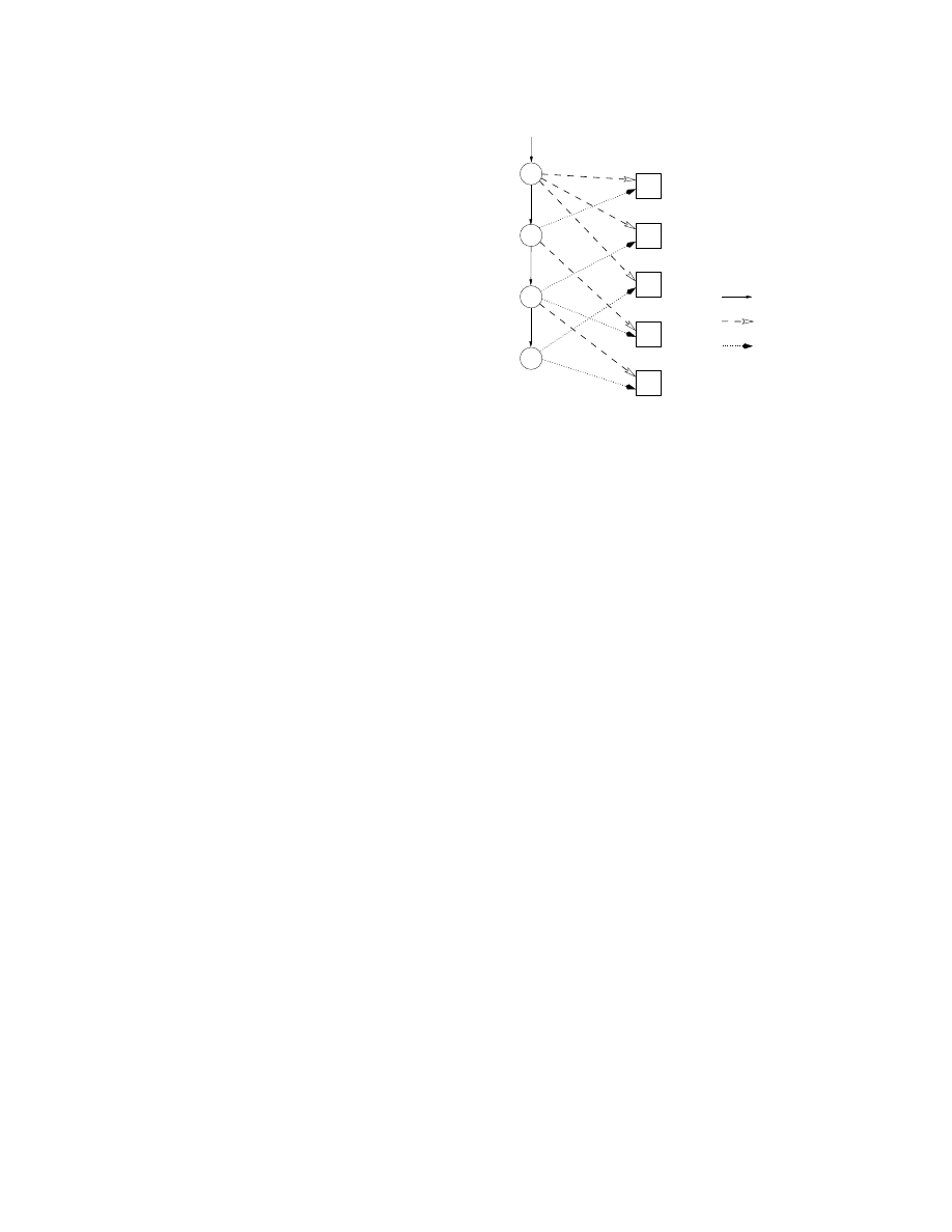
one. This is illustrated by Figure 6, where dashed lines
indicate which memory regions are unpacked by a phase
while dotted lines show the memory regions a phase ex-
ecutes. Phase φ

0

unpacks three memory regions: A, B,

and C. The next phase, φ

1

, executes only one of these

(region A), and unpacks a fourth region, D. The fol-
lowing phase, φ

2

, executes regions B (unpacked by φ

0

)

and D (unpacked by φ

1

), and unpacks region E. Fi-

nally, phase φ

3

executes region C (unpacked by φ

0

) and

E (unpacked by φ

2

). In this example, phase φ

0

unpacks

certain regions of memory that are executed, not by the
next phase φ

1

, but rather by subsequent phases (φ

2

and

φ

3

). We refer to this kind of unpacking as “way-ahead-

of-time (WAT) unpacking.”

WAT-unpacking can be problematic for dynamic mal-

ware analysis tools since it effectively requires that the
tools maintain a complete history of a program’s un-
packing behavior, which can be expensive due to the ad-
ditional memory requirements. In practice, such tools
sometimes make the simplifying assumption that each
phase only unpacks code that is used by the next phase,
i.e., that WAT-unpacking does not take place. This can
compromise soundness by causing some unpacked code
to fail to be detected, as in the case of the Renovo dy-
namic analysis tool [15]. On the other hand, if a static
analysis can guarantee the absence of WAT-unpacking
in a malware executable, subsequent dynamic analyses
of that executable can safely ignore its unpacking his-
tory, thereby improving efficiency significantly without
losing soundness.

WAT-unpacking can be detected by static analysis of

program evolution graphs via a straightforward adapta-
tion of the notion of def-use chains [2]. Using the exec
and write sets for the vertices of a program evolution
graph, we can construct “def-exec chains,” which are
exactly analogous to the traditional static analysis no-
tion of def-use chains and links each modification of a
location (obtainable from the write set of each vertex)
to all of its “uses” (obtainable from the exec set of each
vertex). It is then straightforward to determine whether a
location modified by one phase (vertex) v

1

in a program

evolution graph is used by some other phase (vertex) v

2

where v

2

is not an immediate successor of v

1

.

6.3

Conditionally Activated Unpacking

There are situations where either the unpacker or the

unpacked code may be activated conditionally based on

the value of some input. Examples of such behavior in-
clude the use of anti-monitoring and anti-virtualization
defenses [4, 6, 14, 19], where the malware does not re-
veal itself if it determines that its execution is being
watched; “time bombs” and “logic bombs,” where the
activation occurs only on specific dates (time bombs)
or due to some specific environmental trigger (logic
bombs); and bots that activate specific components of
their payload only when they receive the appropriate
command from a botmaster [10]. We can use static anal-
ysis to identify such situations:

Proposition 6.1 Given a program P containing some
dynamic unpacking code C and a conditional branch B,
the dynamic unpacker code C is conditionally activated
by B if the following hold:

1. the test expression e is computed from a value read

in by an input instruction ‘I

≡ ‘input ⇒

MEM

[e]’;

2. one of the targets of the branch instruction B leads

to C; and

3. the other target of B does not lead to C without

first going through the input instruction I.

The reason for the third condition is that some mal-

ware, such as a bot, may simply sit in a loop, repeatedly
reading in commands and checking to see if any of them
direct it to activate the unpacker code.

The detection of dynamic defenses in this manner can

give security researchers information about the location
and nature of conditionally activated unpackers, thereby
allowing them to take countermeasures if they choose to
use dynamic analysis.

6.4

Cross-Phase Code Analysis

A number of researchers have described techniques

for identifying malware based on examining its code for
incriminating patterns, actions or behaviors. Most mod-
ern anti-virus products use “generic decryptors” to deal
with polymorphic viruses. The idea here is to emulate
the malware code for some amount of time, with the
expectation that this will allow enough of the malware
payload to become unpacked that it can be detected sim-
ply by scanning the contents of memory for telltale byte
sequences [20]. Christodorescu et al. propose a more
general scheme that uses instruction sequence templates
to specify certain kinds of malicious behavior [8]. A sig-
nificant drawback with a great deal of such work is that
they assume that “enough” of the code of the candidate
binary will be available at one time for analysis. This

11

assumption can make it possible for a malware instance
to evade dynamic security analysis tools by taking its
actions and distributing them across multiple unpacking
phases, so that no single phase exposes very much of the
malware code.

These problems can be mitigated by static analysis of

malware code where the entire program evolution graph
is available for analysis. As a simple example, the mal-
ware detection approach of Christodorescu et al. [8] can
be extended to deal with multiple unpacking phases as
follows:

Given an executable program P with program
evolution graph G

= (V, E), a malware tem-

plate τ matches P if either of the following
hold:

1. there is some vertex v

∈ V such that τ

matches v; or

2. there exists a path v

1

, . . . , v

n

in G such

that τ matches the result of concatenat-
ing the code sequences for v

1

, . . . , v

n

.

7

Related Work

The only other work we are aware of that gives a for-

mal semantics for self-modifying code is a recent paper
by Cai et al. [5]. Their goals, namely, verification of
code that is self-modifying but not in a “bad” way, are
very different from ours, namely, static analysis of pro-
grams that may be malicious. The two approaches also
differ considerably in their technical details: Cai et al.
describe an approach based on Hoare logic that they use
to reason about self-modifying code, while our approach
is based on a trace semantics.

Dalla Preda et al. have discussed the use of abstract

interpretation, based on a low-level trace semantics, to
reason about low-level code obfuscations used by mal-
ware [11]. They do not focus on dynamic code modifi-
cations, but assume instead that the program has been
unpacked and correctly disassembled and is available
for analysis; their goal is to use abstract interpretation
to hide the effects of code obfuscations used by mal-
ware, and to use such abstract interpretations to reason
about the soundness and completeness of malware de-
tectors. By contrast, we focus on the actual semantics of
self-modifying code; our goal is to use this semantics as
a basis for constructing behavioral models for, and rea-
soning about, self-modifying programs. The two works
are orthogonal in the sense that the behavioral models
constructed using the approach described here could be

used as input to the techniques described by Dalla Preda
et al..

Christodorescu et al. have proposed incorporating

some knowledge of instruction semantics into virus
scanners to get around simple code obfuscations used
by malware [8]. The semantic information they propose
to use is much simpler than that presented here, and is
based on a notion of “templates,” which are instruction
sequences with place-holders for registers and constants.
They do not consider the semantic issues raised by code
self-modification, but assume that the malware has been
unpacked and is available for analysis. This work is
similarly orthogonal to that described here, and (as dis-
cussed in Section 6.4) could be generalized using our
behavioral models.

There is a large body of literature on malware detec-

tion and analysis; Szor gives a comprehensive summary
[20]. These approaches typically use dynamic analysis,
e.g., via generic decryptors, to deal with runtime code
modification.

8

Conclusions

The rapid growth in the incidence of malware has

made their detection and analysis of fundamental im-
portance in computer system security. Most malware
instances encountered today use packed (i.e., encrypted
or compressed) payloads in an attempt to avoid detec-
tion, unpacking the payloads at runtime via dynamic
code modification. Modern malware detectors use dy-
namic analysis to get around this, but this approach has
the drawback that it may not be able to detect condition-
ally unpacked code, e.g., due to anti-debugging defenses
in the malware or because the malware payload is acti-
vated only on a specific date or time or in response to
some specific command.

This paper describes an approach that complements

such dynamic techniques via static analysis of malware
code. We present a formal semantics that can cope with
self-modifying code, then use this to develop the notion
of a phase-based concrete semantics that describes how
a program’s code evolves due to dynamic code modifi-
cations. We then discuss how this concrete semantics
can be statically approximated. Our ideas can be used to
understand some aspects of the behavior of dynamically
modified code, e.g., the use of anti-monitoring defenses,
and also to statically approximate the code that is un-
packed at runtime.

12

References

[1] A.-R. Adl-Tabatabai, Michał Cierniak, Guei-Yuan

Lueh, Vishesh M. Parikh, and James M. Stichnoth.
Fast, effective code generation in a just-in-time
Java compiler. In Proceedings of the ACM SIG-
PLAN ’98 Conference on Programming Language
Design and Implementation, pages 280–290, June
1998.

[2] A. V. Aho, R. Sethi, and J. D. Ullman. Compil-

ers – Principles, Techniques, and Tools. Addison-
Wesley, Reading, Mass., 1985.

[3] V. Bala, E. Duesterwald, and S. Banerjia.

Dy-

namo: A transparent dynamic optimization sys-
tem. In SIGPLAN ’00 Conference on Program-
ming Language Design and Implementation, pages
1–12, June 2000.

[4] Black Fenix. Black Fenix’s anti-debugging tricks.

http://in.fortunecity.com/skyscraper/browser/12/sicedete.html

.

[5] H. Cai, Z. Shao, and A. Vaynberg. Certified self-

modifying code. In Proc. 2007 ACM SIGPLAN
conference on Programming language design and
implementation (PLDI ’07), pages 66–77, June
2007.

[6] S. Cesare. Linux anti-debugging techniques (fool-

ing the debugger), January 1999. VX Heavens.

http://vx.netlux.org/lib/vsc04.html

.

[7] K. Chiang and L. Lloyd. A case study of the Ru-

stock rootkit and spam bot. In Proc. HotBots ’07:
First Workshop on Hot Topics in Understanding
Botnets. Usenix, April 2007.

[8] M. Christodorescu, S. Jha, S. A. Seshia, D. Song,

and R. E. Bryant. Semantics-aware malware detec-
tion. In Proc. Usenix Security ’05, August 2005.
To appear.

[9] Mihai Christodorescu, Johannes Kinder, Somesh

Jha, Stefan Katzenbeisser, and Helmut Veith. Mal-
ware normalization. Technical Report 1539, Uni-
versity of Wisconsin, Madison, Wisconsin, USA,
November 2005.

[10] E. Cooke, F. Jahanian, and Danny McPherson.

The zombie roundup: Understanding, detecting,
and disrupting botnets.

In Proc. Workshop on

Steps to Reducing Unwanted Traffic on the Inter-
net (SRUTI’05), July 2005.

[11] M. Dalla Preda, M. Christodorescu, S. Jha, and

S. Debray. A semantics-based approach to mal-
ware detection. ACM Transactions on Program-
ming Languages and Systems, 2008. To appear.
(Preliminary version appeared in Proc. 34th An-
nual ACM SIGPLAN-SIGACT Symposium on Prin-
ciples of Programming Languages (POPL’07),
Jan. 2007).

[12] S. K. Debray, R. Muth, and M. Weippert. Alias

analysis of executable code. In Proc. 25th ACM
Symposium on Principles of Programming Lan-
guages (POPL-98), pages 12–24, January 1998.

[13] M. Fernandez and R. Espasa.

Speculative alias

analysis for executable code. In Proc. 11th Inter-
national Conference on Parallel Architectures and
Compilation Techniques (PACT), pages 222–231,
September 2002.

[14] Lord Julus. Anti-debugging in win32, 1999. VX

Heavens.

http://vx.netlux.org/lib/vlj05.html

.

[15] M. G. Kang, P. Poosankam, and H. Yin. Renovo:

A hidden code extractor for packed executables. In
Proc. Fifth ACM Workshop on Recurring Malcode
(WORM 2007), November 2007.

[16] M. Leone and P. Lee. A declarative approach to

run-time code generation. In Proc. Workshop on
Compiler Support for System Software (WCSSS),
February 1996.

[17] J. Maebe and K. De Bosschere. Instrumenting self-

modifying code. In Proc. Fifth International Work-
shop on Automated Debugging (AADEBUG2003),
pages 103–113, September 2003.

[18] F. No¨el, L. Hornof, C. Consel, and J. L. Lawall.

Automatic, template-based run-time specializa-
tion: Implementation and experimental study. In
Proc. 1998 International Conference on Computer
Languages, pages 132–142, 1998.

[19] J. Rutkowska.

Red pill... or how to de-

tect VMM using (almost) one cpu instruction.
http://invisiblethings.org/papers/redpill.html.

[20] P. Sz¨or. The Art of Computer Virus Research and

Defense. Symantek Press, February 2005.

13