
arXiv:gr-qc/0103023 v1 8 Mar 2001
Introduction to relativistic astrophysics and
cosmology through Maple
Vladimir L. Kalashnikov
20th April 2001
Belarussian Polytechnical Academy
kalashnikov vl@mailru.com
www.geocities.com/optomaplev
Abstract
The basics of the relativistic astrophysics including the celestial
mechanics in weak field, black holes and cosmological models are illus-
trated and analyzed by means of Maple 6
Application Areas/Subjects: Science, Astrophysics, General Relativity, Ten-
sor Analysis, Differential geometry, Differential equations
1
Contents
3
2 Relativistic celestial mechanics in weak gravitational field
3
Introduction . . . . . . . . . . . . . . . . . . . . . . . . . . . .
3
Schwarzschild metric . . . . . . . . . . . . . . . . . . . . . . .
3
Equations of motion . . . . . . . . . . . . . . . . . . . . . . .
6
Light ray deflection . . . . . . . . . . . . . . . . . . . . . . . .
10
Planet’s perihelion motion . . . . . . . . . . . . . . . . . . . .
13
Conclusion . . . . . . . . . . . . . . . . . . . . . . . . . . . .
22
3 Relativistic stars and black holes
22
Introduction . . . . . . . . . . . . . . . . . . . . . . . . . . . .
22
Geometric units . . . . . . . . . . . . . . . . . . . . . . . . . .
23
Relativistic star . . . . . . . . . . . . . . . . . . . . . . . . . .
23
Degeneracy stars and gravitational collapse . . . . . . . . . .
40
Schwarzschild black hole . . . . . . . . . . . . . . . . . . . . .
47
om black hole (charged black hole) . . . . . .
55
Kerr black hole (rotating black hole) . . . . . . . . . . . . . .
63
Conclusion . . . . . . . . . . . . . . . . . . . . . . . . . . . .
68
68
Introduction . . . . . . . . . . . . . . . . . . . . . . . . . . . .
68
Robertson-Walker metric . . . . . . . . . . . . . . . . . . . .
69
Standard models . . . . . . . . . . . . . . . . . . . . . . . . .
80
Einstein static . . . . . . . . . . . . . . . . . . . . . .
86
Einstein-de Sitter . . . . . . . . . . . . . . . . . . . . .
87
de Sitter and anti-de Sitter . . . . . . . . . . . . . . .
88
Closed Friedmann-Lemaitre . . . . . . . . . . . . . . .
90
Open Friedmann-Lemaitre . . . . . . . . . . . . . . . .
93
Expanding spherical and recollapsing hyperbolical uni-
verses . . . . . . . . . . . . . . . . . . . . . . . . . . .
96
Bouncing model . . . . . . . . . . . . . . . . . . . . .
98
Our universe (?) . . . . . . . . . . . . . . . . . . . . .
99
Beginning . . . . . . . . . . . . . . . . . . . . . . . . . . . . . 100
4.4.1
Bianchi models and Mixmaster universe . . . . . . . . 100
Inflation . . . . . . . . . . . . . . . . . . . . . . . . . . 117
123
2
1
Introduction
A rapid progress of the observational astrophysics, which resulted from the
active use of orbital telescopes, essentially intensifies the astrophysical re-
searches at the last decade and allows to choose the more definite direc-
tions of further investigations. At the same time, the development of high-
performance computers advances in the numerical astrophysics and cosmol-
ogy. Against a background of these achievements, there is the renascence of
analytical and semi-analytical approaches, which is induced by new genera-
tion of high-efficient computer algebra systems.
Here we present the pedagogical introduction to relativistic astrophysics
and cosmology, which is based on computational and graphical resources
of Maple 6. The pedagogical aims define the use only standard functions
despite the fact that there are the powerful General Relativity (GR) oriented
extensions like GRTensor [1]. The knowledge of basics of GR and differential
geometry is supposed. It should be noted, that our choice of metric signature
(+2) governs the definitions of Lagrangians and energy-momentum tensors.
The computations in this worksheet take about of 6 min of CPU time (PIII-
500) and 9 Mb of memory.
2
Relativistic celestial mechanics in weak gravita-
tional field
2.1
Introduction
The first results in the GR-theory were obtained without exact knowledge
of the field equations (Einstein’s equations for space-time geometry). The
leading idea was the equivalence principle based on the equality of iner-
tial and gravitational masses. We will demonstrate here that the natural
consequences of this principle are the Schwarzschild metric and the basic
experimental effects of GR-theory in weak gravitational field, i. e. planet’s
orbit precession and light ray deflection (see [2]).
2.2
Schwarzschild metric
Let us consider the centrally symmetric gravitational field, which is produced
by mass M. The small cell K
∞
falls along x -axis on the central mass. In the
agreement with the equivalence principle, the uniformly accelerated motion
3
locally compensates the gravitational force hence there is no a gravitational
field in the free falling system K
∞
. This results in the locally Lorenzian
metric with linear element (c is the velocity of light):
d s
2
= d x
∞
2
+ d y
∞
2
+ d z
∞
2
- c
2
d t
∞
2
The velocity v and radial coordinate r are measured in the spherical system
K, which are connected with central mass. It is natural, the observer in
this motionless system ”feels” the gravitational field. Since the first sys-
tem moves relatively second one there are the following relations between
coordinates:
d x
∞
=
dr
√
1
−β
2
( β =
v
c
)
d t
∞
=
p
1
− β
2
dt
d y
∞
=rd θ
d z
∞
=r sin(θ) d φ
The first and second relations are the Lorentzian length shortening and time
slowing down in the moving system. As result, K
∞
from K looks as:
d s
2
= (1
− β
2
)
(
−1)
d r
2
+ r
2
(d θ
2
+ sin(θ)
2
d φ
2
) - c
2
(1 - β
2
)d t
2
The sense of the additional terms in metric has to connect with the char-
acteristics of gravitational field. What is the energy of K
∞
in K ? If the
mass of K
∞
is m, and m
0
is the rest mass, the sum of kinetic and potential
energies is:
4
>
restart:
>
with(plots):
>
(m - m0)*c^2 - G*M*m/r=0;#energy conservation law\
>
(we suppose that the Newtonian law of gravitation\
>
is correct in the first approximation), G is\
>
the gravitational constant
>
%/(m*c^2):
>
subs( m=m0/sqrt(1-beta^2),% ):# relativistic mass
>
expand(%);
>
solve( %,sqrt(1-beta^2) ):
>
sqrt(1-beta^2) = expand(%);
>
1-beta^2 =
>
taylor((1-subs(op(2,%)=alpha/r,rhs(%)))^2,alpha=0,2);\
>
#alpha=G*M/c^2, we use the first-order approximation \
>
on alpha
(m
− m0 ) c
2
−
G M m
r
= 0
1
−
q
1
− β
2
−
G M
c
2
r
= 0
q
1
− β
2
= 1
−
G M
c
2
r
1
− β
2
= 1
− 2
1
r
α + O(α
2
)
The last results in:
d s
2
=
dr
2
1
−
2 α
r
+ r
2
(d θ
2
+ sin(θ)
2
d φ
2
) - c
2
(1 -
2 α
r
)d t
2
This linear element describes the so-called Schwarzschild metric. In the
first-order approximation:
>
taylor(
>
d(r)^2/(1-2*alpha/r)+r^2*(d(theta)^2+sin(theta)^2*\
>
d(phi)^2)-c^2*(1-2*alpha/r)*d(t)^2, alpha=0, 2 ):
>
convert( % , polynom ):
>
metric := d(s)^2 = collect( % ,
{d(r)^2, d(t)^2} );
metric := d(s)
2
=
(
−c
2
+
2 c
2
α
r
) d(t)
2
+ (1 +
2 α
r
) d(r)
2
+ r
2
(d(θ)
2
+ sin(θ)
2
d(φ)
2
)
5
2.3
Equations of motion
Let us consider a motion of the small unit mass in Newtonian gravitational
potential Φ = -
G M
r
. Lagrangian describing the motion in centrally sym-
metric field is:
>
L :=\
>
(diff(r(t),t)^2 + r(t)^2*diff(theta(t),t)^2)/2\
>
+ G*M/r(t);
L :=
1
2
(
∂
∂t
r(t))
2
+
1
2
r(t)
2
(
∂
∂t
θ(t))
2
+
G M
r(t)
The transition to Schwarzschild metric transforms the time and radial differ-
entials of coordinates (see, for example, [3, 4]): dr –> (1 +
α
r
)dr and dt –>
(1 +
α
r
)
(
−1)
dt (it should be noted, that the replacement will be performed
for differentials, not coordinates, and we use the weak field approximation
for square-rooting):
>
L_n := collect(\
>
expand(\
>
subs(\
>
{diff(r(t),t)=gamma(r(t))^2*diff(r(t),t),\
>
diff(theta(t),t)=gamma(r(t))*diff(theta(t),t)
}, L ) ),\
>
{diff(r(t),t)^2, diff(theta(t),t)^2});# modified\
>
Lagrangian, gamma(r) = 1+alpha/r(t)
L n :=
1
2
γ(r(t))
4
(
∂
∂t
r(t))
2
+
1
2
r(t)
2
γ(r(t))
2
(
∂
∂t
θ(t))
2
+
G M
r(t)
Next step for the obtaining of the equations of motion from Lagrangian is
the calculation of the force
∂
∂x
L(x, y) and the momentum
∂
∂y
L(x, y) , where
y=
∂
∂t
x :
6
>
e1 := Diff(Lagrangian(r, Diff(r,t)), r) = \
>
diff(subs(r(t) = r,L_n),r);#first component of force
>
e2 := Diff(Lagrangian(r, Diff(r,t)), Diff(r,t)) = \
>
subs(x=diff(r(t),t), diff(subs(diff(r(t),t)=x, L_n),\
>
x));#first component of momentum
>
e3 := Diff(Lagrangian(theta, Diff(theta,t)), theta) =
>
diff(subs(theta(t) = theta, L_n), theta);#second\
>
component of force
>
e4 := Diff(Lagrangian(theta, Diff(theta,t)),\
>
Diff(theta,t)) = subs(y=diff(theta(t),t),\
>
diff(subs(diff(theta(t),t)=y, L_n), y));#second\
>
component of momentum
e1 :=
∂
∂r
Lagrangian(r,
∂
∂t
r) =
2 γ(r)
3
(
∂
∂t
r)
2
(
∂
∂r
γ(r)) + r γ(r)
2
(
∂
∂t
θ(t))
2
+ r
2
γ(r) (
∂
∂t
θ(t))
2
(
∂
∂r
γ(r))
−
G M
r
2
e2 := Diff(Lagrangian(r,
∂
∂t
r),
∂
∂t
r) = γ(r(t))
4
(
∂
∂t
r(t))
e3 :=
∂
∂θ
Lagrangian(θ,
∂
∂t
θ) = r(t)
2
γ(r(t))
2
(
∂
∂t
θ) (
∂
2
∂θ ∂t
θ)
e4 := Diff(Lagrangian(θ,
∂
∂t
θ),
∂
∂t
θ) = r(t)
2
γ(r(t))
2
(
∂
∂t
θ(t))
The equations of motion are the so-called Euler-Lagrange equations
∂
2
∂t ∂y
L(x, y)
−
∂
∂x
L(x, y) = 0 (in fact, these equations are the second New-
ton’s law and result from the law of least action). Now let us write the
equations of motion in angular coordinates. Since e3 = 0 due to an equality
to zero of the mixed derivative, we have from e4 the equation of motion
∂
2
∂t ∂y
2
L(r, θ, y
1
, y
2
) -
∂
∂θ
L(r, θ, y
1
, y
2
) = 0 ( y
1
=
∂
∂t
r , y
2
=
∂
∂t
θ ) in the
form:
>
Eu_Lagr_1 := Diff(rhs(e4),t) = 0;
Eu Lagr 1 :=
∂
∂t
r(t)
2
γ(r(t))
2
(
∂
∂t
θ(t)) = 0
Hence
7

r(t)
2
γ(r(t))
2
(
∂
∂t
θ(t)) = H = const
>
sol_1 := Diff(theta(t),t) = solve(\
>
gamma^2*diff(theta(t),t)/u(theta)^2 = H,\
>
diff(theta(t),t) );#u=1/r is the new variable
sol 1 :=
∂
∂t
θ(t) =
H u(θ)
2
γ
2
The introduced replacement u=
1
r
leads to the next relations:
>
Diff(r(t), t) = diff(1/u(t),t);
>
Diff(r(t), t) = diff(1/u(theta),theta)*\
>
diff(theta(t),t);# change of variables
>
sol_2 := Diff(r(t), t) =\
>
subs(diff(theta(t),t) = rhs(sol_1),\
>
rhs(%));# the result of substitution of\
>
above obtained Euler-Lagrange equation
∂
∂t
r(t) =
−
∂
∂t
u(t)
u(t)
2
∂
∂t
r(t) =
−
(
∂
∂θ
u(θ)) (
∂
∂t
θ(t))
u(θ)
2
sol 2 :=
∂
∂t
r(t) =
−
(
∂
∂θ
u(θ)) H
γ
2
The last result will be used for the manipulations with second Euler-Lagrange
equation
∂
2
∂t ∂y
1
L(r, θ, y
1
, y
2
) -
∂
∂r
L(r, θ, y
1
, y
2
) = 0. We have for the right-
hand side of e2 :
>
Diff( subs(
{diff(r(t),t)=rhs(%),gamma(r(t))=gamma},\
>
rhs(e2)), t);
∂
∂t
(
−γ
2
(
∂
∂θ
u(θ)) H)
and can rewrite this expression:
8
>
-2*gamma*H*diff(1+alpha/r(t),t)*diff(u(theta),theta) -\
>
H*gamma^2*diff(u(theta),theta$2)*diff(theta(t),t);#from\
>
the previous expression, definition of gamma and\
>
definition of derivative of product
>
first_term := subs(
{r(t)=1/u(theta),\
>
diff(theta(t),t)=rhs(sol_1)
},\
>
subs(diff(r(t),t) = rhs(sol_2),%));# this is \
>
a first term in second Euler-Lagrange equation
2
γ H α (
∂
∂t
r(t)) (
∂
∂θ
u(θ))
r(t)
2
− H γ
2
(
∂
2
∂θ
2
u(θ)) (
∂
∂t
θ(t))
first term :=
−2
H
2
α u(θ)
2
(
∂
∂θ
u(θ))
2
γ
− H
2
(
∂
2
∂θ
2
u(θ)) u(θ)
2
e1 results in:
>
2*gamma(r)^3*diff(r(t),t)^2*diff(gamma(r),r) + \
>
r*gamma(r)^2*diff(theta(t),t)^2 + \
>
r^2*gamma(r)*diff(theta(t),t)^2*diff(gamma(r),r) - \
>
G*M/(r^2);# This is e1
>
subs(\
>
{diff(r(t),t) = rhs(sol_2), diff(gamma(r),r) =\
>
diff(1+alpha/r,r),\
>
diff(theta(t),t) = rhs(sol_1)
},\
>
%):# we used the expressions for diff(r(t),t), gamma(r)\
>
and the first equation of motion
>
subs(gamma(r) = gamma, %):
>
second_term := subs(r = 1/u(theta), %);
2 γ(r)
3
(
∂
∂t
r(t))
2
(
∂
∂r
γ(r)) + r γ(r)
2
(
∂
∂t
θ(t))
2
+ r
2
γ(r) (
∂
∂t
θ(t))
2
(
∂
∂r
γ(r))
−
G M
r
2
second term :=
−2
H
2
α u(θ)
2
(
∂
∂θ
u(θ))
2
γ
+
u(θ)
3
H
2
γ
2
−
H
2
u(θ)
4
α
γ
3
− G M u(θ)
2
And finally:
>
Eu_Lagr_2 := expand( simplify(first_term -\
>
second_term)/u(theta)^2/H^2);
9
Eu Lagr 2 :=
−(
∂
2
∂θ
2
u(θ))
−
u(θ)
γ
2
+
u(θ)
2
α
γ
3
+
G M
H
2
In the first-order approximation:
>
gamma^n = taylor((1+alpha*u)^n, alpha=0,2);
γ
n
= 1 + n u α + O(α
2
)
So
>
taylor( subs(gamma = 1+alpha*u(theta),Eu_Lagr_2),\
>
alpha=0,2 ):
>
basic_equation := convert(%, polynom) = 0;
basic equation :=
−(
∂
2
∂θ
2
u(θ))
− u(θ) +
G M
H
2
+ 3 u(θ)
2
α = 0
2.4
Light ray deflection
In the beginning the obtained equation will be used for the search of the
light ray deflection in the vicinity of a star. The fundamental consideration
has to be based on the condition of null geodesic line d s
2
=0 for light, but
we simplify a problem and consider the trajectory of the particle moving
from the infinity. In this case H=
∞ .
>
eq_def := subs(G*M/(H^2)=0,basic_equation);
eq def :=
−(
∂
2
∂θ
2
u(θ))
− u(θ) + 3 u(θ)
2
α = 0
The free propagation ( α =0) results in:
>
subs(alpha=0, lhs(eq_def)) = 0;
>
sol := dsolve(
{%, u(0) = 1/R, D(u)(0) = 0}, u(theta));
>
# theta is measured from perihelion, where r = R
10

−(
∂
2
∂θ
2
u(θ))
− u(θ) = 0
sol := u(θ) =
cos(θ)
R
That is r=
R
cos(θ)
. The last expression corresponds to the straight ray
passing through point θ =0, r =R. To find the corrected solution in the
gravitational field let substitute the obtained solution into eliminated term
in eq def :
>
-op(1,lhs(eq_def)) - op(2,lhs(eq_def)) =\
>
subs(u(theta)=rhs(sol),op(3,lhs(eq_def)));
>
sol := dsolve(\
>
{%, u(0) = 1/R, D(u)(0) = 0}, u(theta));#corrected\
>
solution in the presence of field
(
∂
2
∂θ
2
u(θ)) + u(θ) = 3
cos(θ)
2
α
R
2
sol := u(θ) =
(
−α + R) cos(θ)
R
2
−
1
2
α cos(2 θ)
R
2
+
3
2
α
R
2
The equation for asymptote lim
θ
→(
π
2
)
u(θ) describes the observed ray.
Then angle of ray deflection is
2 R
r
(symmetrical deflection before and after
perihelion). Hence
>
simplify( 2*subs(
{theta=Pi/2, alpha=G*M/c^2},\
>
rhs(sol))*R );
4
G M
R c
2
This is a correct expression for the light ray deflection in the gravitational
field. For sun we have:
11
>
subs(
{kappa=0.74e-28, M=2e33, R=6.96e10},\
>
4*kappa*M/R/4.848e-6);
>
# in ["],where kappa = G/c^2 [cm/g], \
>
4.848e-6 rad corresponds to 1"
1.754485794
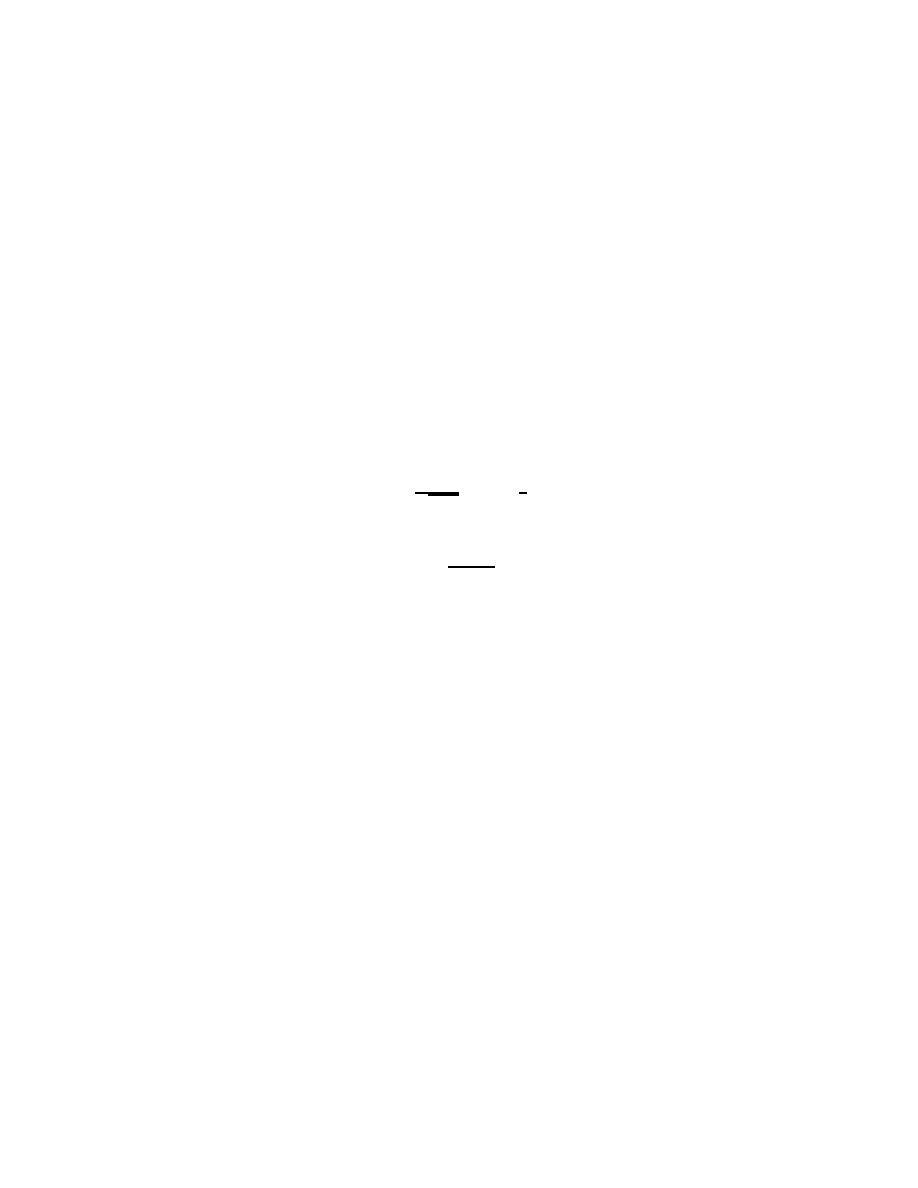
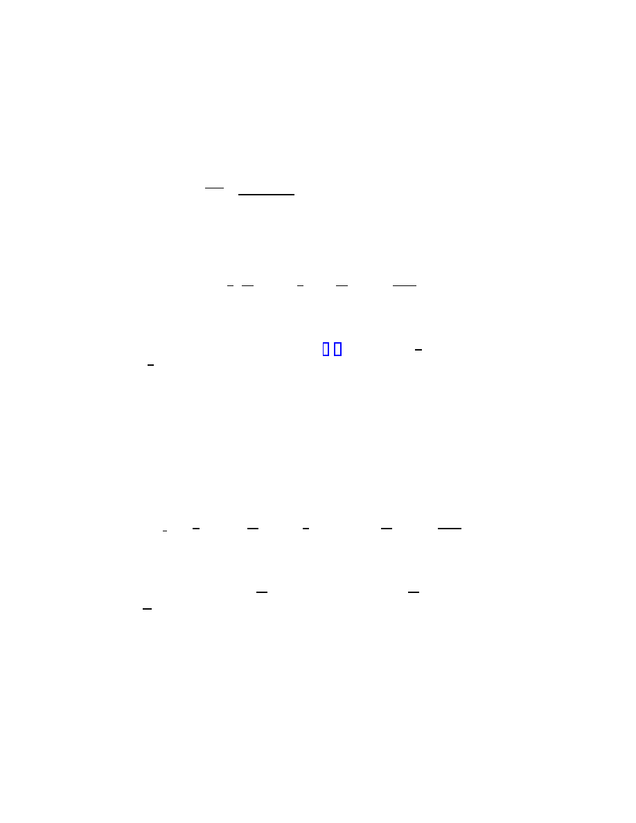
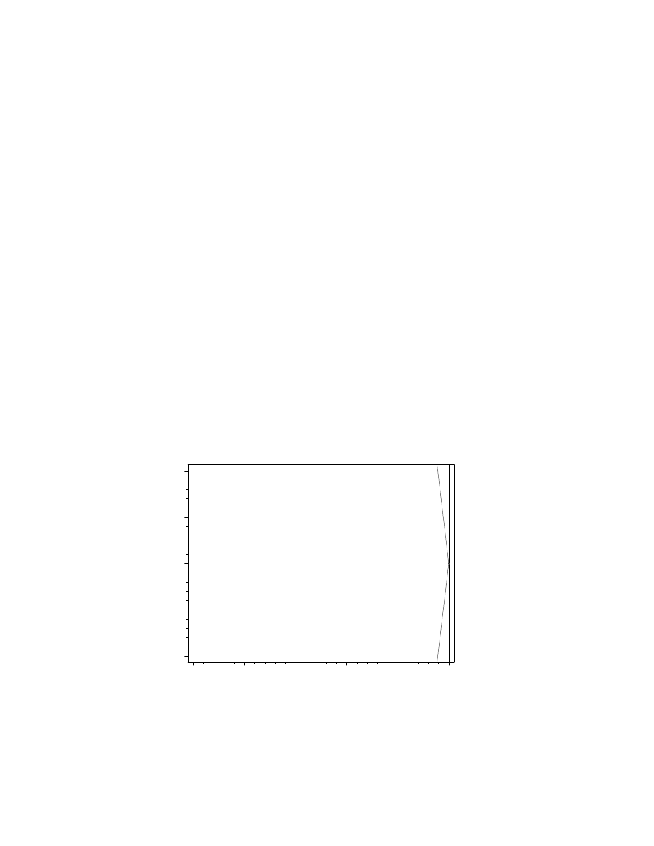
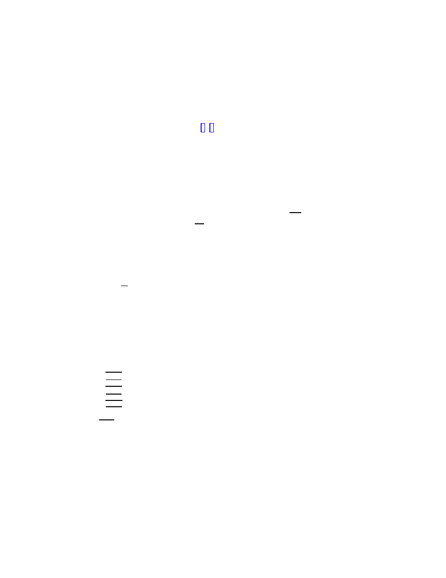
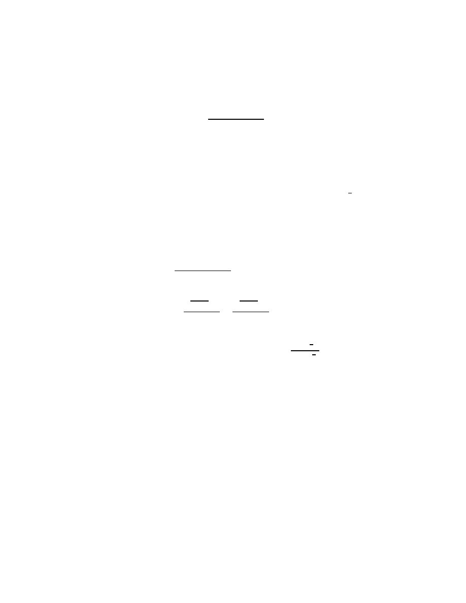
The ray trajectory within Pluto’s orbit distance is presented below:
>
K := (theta, alpha, R) -> 1 /\
>
(-(alpha-R)*cos(theta)/(R^2)-1/2*alpha*cos(2*theta)/\
>
(R^2)+3/2*alpha/(R^2)):
>
S := theta -> K(theta, 2.125e-6, 1):#deflected ray
>
SS := theta -> 1/cos(theta):#ray without deflection
>
p1 := polarplot(\
>
[S,theta->theta,Pi/2..-Pi/2],axes=boxed):
>
p2 :=\
>
polarplot([SS,theta->theta,Pi/2..-Pi/2],\
>
axes=boxed,color=black):
>
display(p1,p2,view=-10700..10700,\
>
title=‘deflection of light ray‘);\
>
#distance of propagation corresponds to\
>
100 AU=1.5e10 km, distance is normalyzed to Sun radius
deflection of light ray
–10000
–5000
0
5000
10000
0
0.2
0.4
0.6
0.8
1
12
2.5
Planet’s perihelion motion
Now we return to basic equation. Without relativistic correction to the
metric ( α =0) the solution is
>
sol :=\
>
dsolve(
{subs({G*M/(H^2)=k,alpha=0},\
>
basic_equation),u(0)=1/R,D(u)(0)=0
},u(theta));
sol := u(θ) = k
−
(k R
− 1) cos(θ)
R
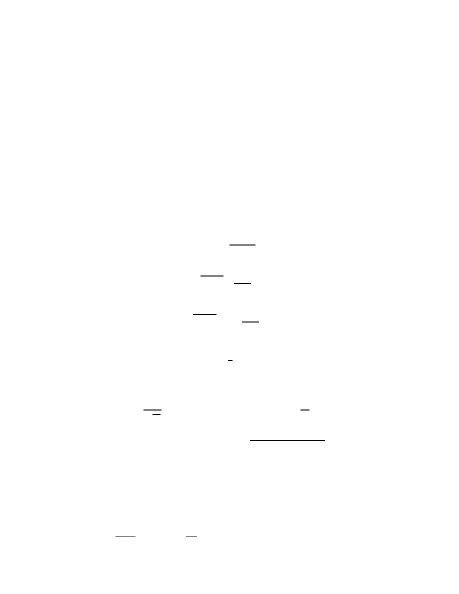
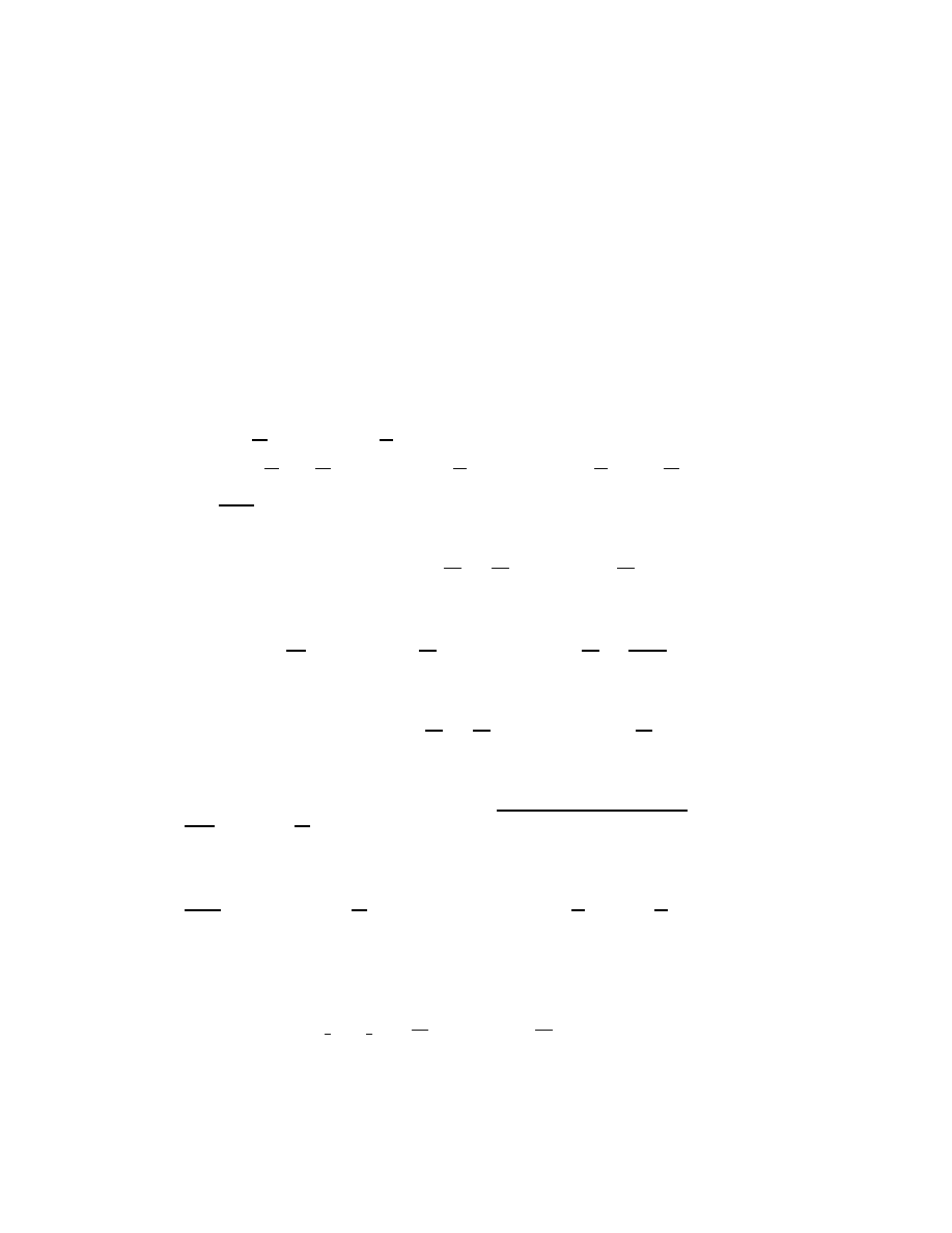
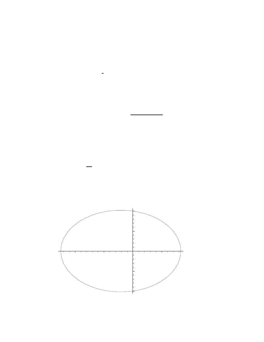
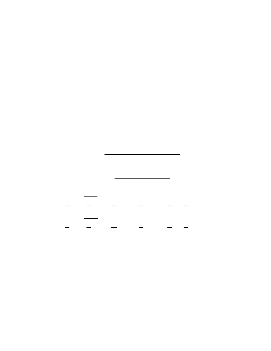
This equation describes an elliptical orbit:
u=k (1+e* cos(θ) ),
where e = (
1
k R
- 1) is the eccentricity. For Mercury k = 0.01, e =
0.2056, R = 83.3
>
K := (theta, k, R) -> 1/(k-(k*R-1)*cos(theta)/R):
>
S := theta -> K(theta, .01, 83.3):
>
polarplot([S,theta->theta,0..2*Pi],\
>
title=‘Orbit of Mercury‘);
Orbit of Mercury
–100
–50
50
100
–100
–50
50
13
The correction to this expression results from the substitution of ob-
tained solution in basic equation.
>
subs(
{G*M/(H^2)=k, 3*u(theta)^2*alpha=\
>
3*alpha*(k*(1+e*cos(theta)))^2
}, basic_equation);
>
dsolve(
{%,u(0)=1/R,D(u)(0)=0},u(theta));
−(
∂
2
∂θ
2
u(θ))
− u(θ) + k + 3 α k
2
(1 + e cos(θ))
2
= 0
u(θ) =
3 α k
2
e cos(θ) + 3 sin(θ) α k
2
e θ +
3
2
α k
2
e
2
−
1
2
α k
2
e
2
cos(2 θ) + k + 3 α k
2
−
(3 α k
2
e R + α k
2
e
2
R + k R + 3 α k
2
R
− 1) cos(θ)
R
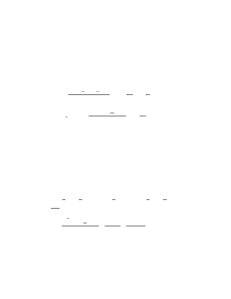
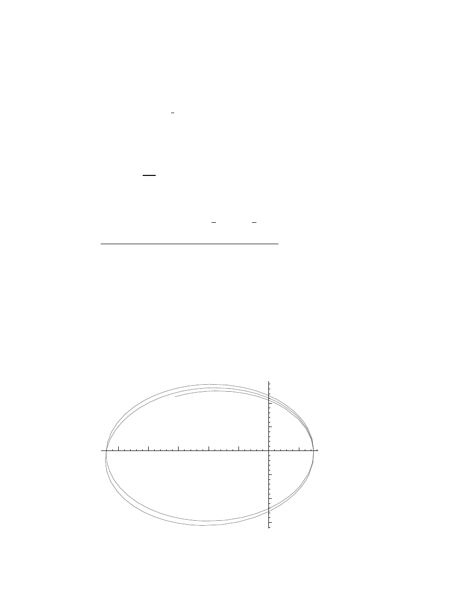
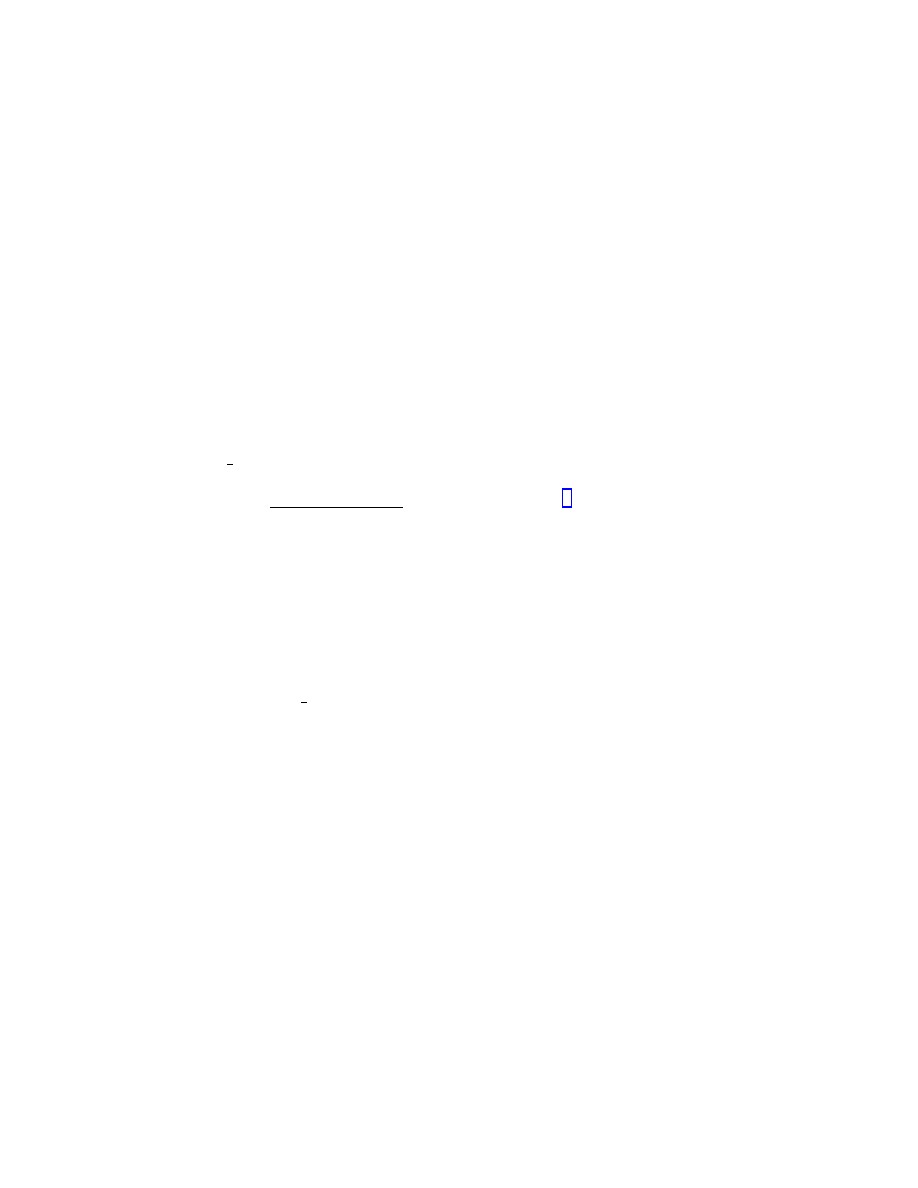
Now it is possible to plot the corrected orbit (we choose the exaggerated
parameters for demonstration of orbit rotation):
>
K := (theta, k, R, alpha, e) -> 1 /\
>
(3*alpha*k^2*e*cos(theta) + \
>
3*sin(theta)*alpha*k^2*e*theta + \
>
3/2*alpha*k^2*e^2 - 1/2*alpha*k^2*e^2*cos(2*theta) +\
>
k + 3*alpha*k^2 - (3*alpha*k^2*e*R + alpha*k^2*e^2*R +\
>
k*R + 3*alpha*k^2*R - 1)*cos(theta)/R):
>
S := theta -> K(theta, .42, 1.5, 0.01, 0.6):
>
polarplot([S,theta->theta,0..4.8*Pi],\
>
title=‘rotation of orbit‘);
rotation of orbit
–3
–2
–1
0
1
2
–5
–4
–3
–2
–1
1
14

Now we try to estimate the perihelion shift due to orbit rotation. Let’s
suppose that the searched solution of basic equation differs from one in the
plane space-time only due to ellipse rotation. The parameter describing this
rotation is ω : u( θ ) = k (1 + e cos(θ
− ω θ) ).
>
subs(
{G*M/(H^2)=k, u(theta)=\
>
k*(1+e*cos(theta-omega*theta))
},\
>
basic_equation):#substitution of approximate solution
>
simplify(%):
>
lhs(%):
>
collect(%, cos(-theta+omega*theta)):
>
coeff(%, cos(-theta+omega*theta)):#the coefficient\
>
before this term gives algebraic equation for omega
>
subs(omega^2=0,%):#omega is the small value and \
>
we don’t consider the quadratic term
>
solve(% = 0, omega):
>
subs(
{alpha = G*M/c^2, k = 1/R/(1+e)},2*Pi*%);#result\
>
is expressed through the minimal distance R between\
>
planet and sun; 2*Pi corresponds to the transition to \
>
circle frequency of rotation
>
subs(R=a*(1-e),%);#result expressed through larger\
>
semiaxis a of an ellipse
6
π G M
c
2
R (1 + e)
6
π G M
c
2
a (1
− e) (1 + e)
Hence for Mercury we have the perihelion shift during 100 years:
>
subs(
{kappa=0.74e-28,M=2e33,a=57.9e11,e=0.2056},\
>
6*Pi*kappa*M/a/(1-e^2)*(100*365.26/87.97)/4.848e-6):\
>
#here we took into account the periods of Earth’s\
>
and Mercury’s rotations
>
evalf(%);#["]
43.08704513
Now we will consider the basic equation in detail [5]. The implicit solu-
tions of this equation are:
15
>
dsolve( subs(G*M/H^2=k, basic_equation), u(theta));
Z
u(θ)
1
√
C1
− a
2
+ 2 k a + 2 a
3
α
d a
− θ − C2 = 0,
Z
u(θ)
−
1
√
C1
− a
2
+ 2 k a + 2 a
3
α
d a
− θ − C2 = 0
Hence, these implicit solutions result from the following equation ( β is the
constant depending on the initial conditions):
>
diff( u(theta), theta)^2 =\
>
2*M*u(theta)^3 - u(theta)^2 + 2*u(theta)*M/H^2 + beta;\
>
# we use the units, where c=1, G=1 (see\
>
definition of the geometrical units in the next part)
>
f := rhs(%):
>
f = 2*M*\
>
( u(theta) - u1 )*( u(theta) - u2 )*( u(theta) - u3 );
(
∂
∂θ
u(θ))
2
= 2 M u(θ)
3
− u(θ)
2
+
2 u(θ) M
H
2
+ β
2 M u(θ)
3
− u(θ)
2
+
2 u(θ) M
H
2
+ β = 2 M (u(θ)
− u1 ) (u(θ) − u2 ) (u(θ) − u3 )
Here u1, u2, u3 are the roots of cubic equation, which describes the ”poten-
tial” defining the orbital motion:
>
fun := rhs(%);
fun := 2 M (u(θ)
− u1 ) (u(θ) − u2 ) (u(θ) − u3 )
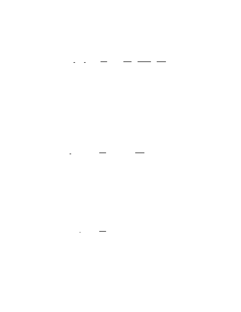
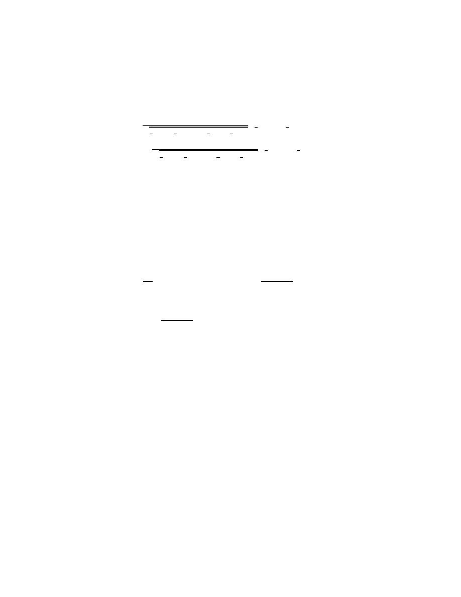
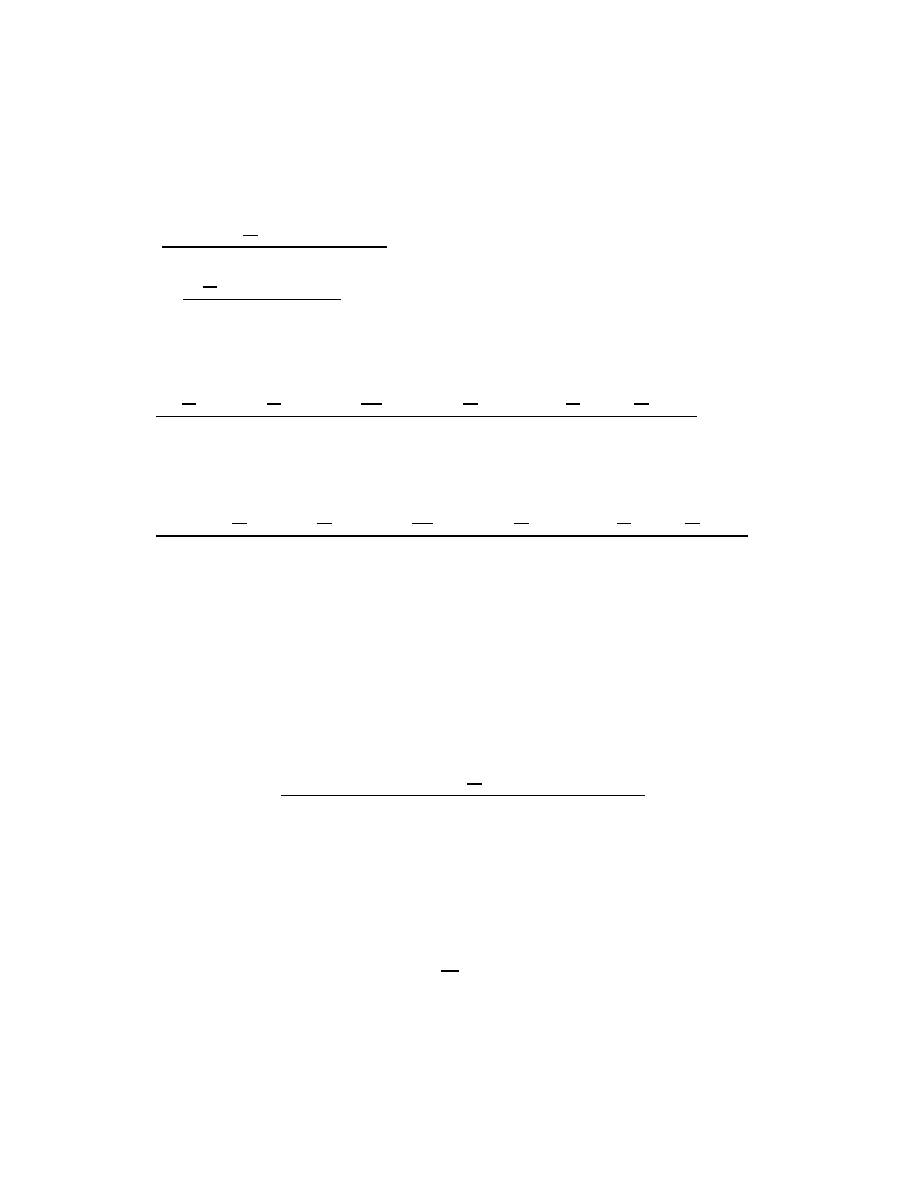
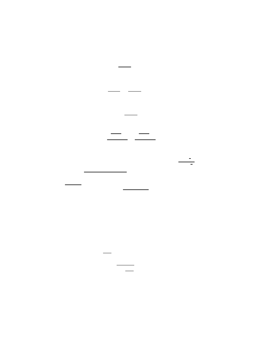
The dependence of this function on u leads to the different types of motion.
The confined motion corresponds to an elliptical orbit
>
plot(subs(
{u3=2, u2=1, u1=0.5, M=1/2},fun),u=0.4..1.1,\
>
title=‘elliptical motion‘, axes=boxed, view=0..0.08);
16
elliptical motion
0
0.01
0.02
0.03
0.04
0.05
0.06
0.07
0.08
0.4
0.5
0.6
0.7
0.8
0.9
1
1.1
u
The next situation with u–>0 (r–>
∞ ) corresponds to an infinite motion:
>
plot(subs(
{u3=2, u2=1, u1=-0.1, M=1/2},fun),u=0..1.1,\
>
title=‘hyperbolical motion‘, axes=boxed, view=0..0.6);
hyperbolical motion
0
0.1
0.2
0.3
0.4
0.5
0.6
0
0.2
0.4
0.6
0.8
1
u
Now we return to the right-hand side of the modified basic equation.
>
f;
17
2 M u(θ)
3
− u(θ)
2
+
2 u(θ) M
H
2
+ β
In this expression, one can eliminate the second term by the substitution u(
θ )= y( θ ) (
2
M
)
(
1
3
)
+
1
6 M
:
>
collect( subs(u(theta) =\
>
(2/M)^(1/3)*y(theta) + 1/(6*M), f),y(theta));
4 y(θ)
3
+
−
1
6
2
(1/3)
(
1
M
)
(1/3)
M
+
2 2
(1/3)
(
1
M
)
(1/3)
M
H
2
y(θ)
−
1
54
1
M
2
+ β +
1
3
H
2
This substitution reduced our equation to canonical form for the Weier-
strass P function [6]:
>
g2 = simplify(coeff(%, y(theta)));
>
g3 = -simplify(coeff(%%, y(theta), 0));
>
diff( y(theta), theta)^2 =\
>
4*y(theta)^3 - g2*y(theta) - g3;
g2 =
1
6
2
(1/3)
(
1
M
)
(1/3)
(
−H
2
+ 12 M
2
)
M H
2
g3 =
−
1
54
−H
2
+ 54 β M
2
H
2
+ 18 M
2
M
2
H
2
(
∂
∂θ
y(θ))
2
= 4 y(θ)
3
− g2 y(θ) − g3
that results in:
>
y(theta) = WeierstrassP(theta, g2, g3);
y(θ) = WeierstrassP(θ, g2 , g3 )
18

In the general case, the potential in the form of three-order polynomial
produces the solution in the form of Jacobi sn-function:
>
Orbit := proc(f, x)
>
print(‘Equation in the form:
u’(theta)^2 =\
>
a[0]*u^3+a[1]*u^2+a[2]*u+a[3]‘):
>
degree(f,x):
>
if(% = 3) then
>
a[0] := coeff(f, x^3):# coefficients of polynomial
>
a[1] := coeff(f, x^2):
>
a[2] := coeff(f, x):
>
a[3] := coeff(f, x, 0):
>
sol := solve(f = 0, x):
>
print(‘Roots of polynomial u[1] < u[2] < u[3]:‘):
>
print(sol[1], sol[2], sol[3]):
>
solution := u[1] + (u[2]-u[1])*JacobiSN(theta*sqrt(\
>
2*M*(u[3]-u[1]) )/2 + delta,\
>
sqrt((u[2]-u[1])/(u[3]-u[1])))^2:
>
print(‘Result through Jacobi sn - function‘):
>
print(u(theta) = solution):
>
else
>
print(‘The polynomial degree is not 3‘)
>
fi
>
end:
Equation in the form :
u
0
(theta)ˆ2 = a[0 ]
∗ uˆ3 + a[1 ] ∗ uˆ2 + a[2 ] ∗ u + a[3 ]
Roots of polynomial u[1 ] < u[2 ] < u[3 ] :
19

1
6
%1
(1/3)
M H
−
1
6
−H
2
+ 12 M
2
M H %1
(1/3)
+
1
6
M
,
−
1
12
%1
(1/3)
M H
+
1
12
(
−H
2
+ 12 M
2
)
M H %1
(1/3)
+
1
6
M
+
1
2
I
√
3
1
6
%1
(1/3)
M H
+
1
6
(
−H
2
+ 12 M
2
)
M H %1
(1/3)
,
−
1
12
%1
(1/3)
M H
+
1
12
(
−H
2
+ 12 M
2
)
M H %1
(1/3)
+
1
6
M
−
1
2
I
√
3
1
6
%1
(1/3)
M H
+
1
6
(
−H
2
+ 12 M
2
)
M H %1
(1/3)
%1 := H
3
− 54 β M
2
H
3
− 18 H M
2
+ 6
√
3
p
−M
2
H
2
+ 16 M
4
− H
6
β + 27 H
6
β
2
M
2
+ 18 H
4
β M
2
M
Result through Jacobi sn
− function
u(θ) = u
1
+ (u
2
− u
1
) JacobiSN(
1
2
θ
√
2
q
M (u
3
− u
1
) + δ,
s
u
2
− u
1
u
3
− u
1
)
2
As u
1
=
1
r
1
and u
2
=
1
r
2
are the small values for the planets ( r
1
and r
2
are
the perihelion and aphelion points) and u
1
+ u
2
+ u
3
=
1
2 M
, we have 2M
u
3
=1 and
>
u(theta) - u[1] =\
>
(u[2] - u[1])*JacobiSN(1/2*theta+delta,0)^2;
u(θ)
− u
1
= (u
2
− u
1
) sin(
1
2
θ + δ)
2
that is the equation of orbital motion (see above) with e =
u
2
−u
1
u
2
+u
1
. u
1
>
0 corresponds to the elliptical motion, u
1
< 0 corresponds to hyperbolical
motion. The period of the orbital motion in the general case:
20
>
(u[2]-u[1])/(u[3]-u[1]):
>
kernel := 2/sqrt((1-t^2)*(1-t^2*%)):#2 in the numerator\
>
corresponds to sn^2-period
>
int(kernel, t=0..1);
2 EllipticK(
s
−
u
2
− u
1
−u
3
+ u
1
)
and can be found approximately for small u
1
and u
2
as result of expansion:
>
series(2*EllipticK(x), x=0,4):
>
convert(%,polynom):
>
subs(x = sqrt( 2*M*(u[2]-u[1]) ), %);
π +
1
2
π M (u
2
− u
1
)
From the expression for u( θ ) and obtained expression for the period of sn
2
we have the change of angular coordinate over period:
>
%/(1/2*sqrt( 2*M*(u[3]-u[1]) )):
>
simplify(%);
1
2
π (2 + M u
2
− M u
1
)
√
2
p
−M (−u
3
+ u
1
)
But
p
2 M (u
3
− u
1
) =
p
1
− 2 M (u
1
− u
2
− u
1
)
≈ 1 + M (2 u
1
+ u
2
) . And
the result is
>
2*Pi*(1 + M*(u[2]-u[1])/2)*(1 + M*(2*u[1]+u[2])):
>
series(%, u[1]=0,2):
>
convert(%,polynom):
>
series(%, u[2]=0,2):
>
convert(%,polynom):
>
expand(%):
>
expand(%-op(4,%)):
>
factor(%);
π (2 + 3 M u
1
+ 3 M u
2
)
The deviation of the period from 2 π causes the shift of the perihelion over
21
one rotation of the planet around massive star.
>
simplify(%-2*Pi):
>
subs(
{u[1]=1/r[1], u[2]=1/r[2]}, %):
>
subs(
{r[1]=a*(1+e), r[2]=a*(1-e)},G*%/c^2):# we\
>
returned the constants G and c
>
simplify(%);
−6
G π M
a (1 + e) (
−1 + e) c
2
This result coincides with the expression, which was obtained on the basis
of approximate solution of basic equation. From the Kepler’s low we can
express this result through orbital period:
>
subs(M=4*Pi^2*a^3/T^2, %):# T is the orbital period
>
simplify(%);
−24
G π
3
a
2
T
2
(1 + e) (
−1 + e) c
2
2.6
Conclusion
So, we found the expression for the Schwarzschild metric from the equiva-
lence principle without introducing of the Einstein’s equations. On this ba-
sis and from Euler-Lagrange equations we obtained the main experimental
consequences of GR-theory: the light ray deflection and planet’s perihelion
motion.
3
Relativistic stars and black holes
3.1
Introduction
The most wonderful prediction of GR-theory is the existence of black holes,
which are the objects with extremely strong gravitational field. The in-
vestigation of these objects is the test of our understanding of space-time
structure. We will base our consideration on the analytical approach that
demands to consider only symmetrical space-times. But this restriction does
22
not decrease the significance of the obtained data because of the rich struc-
ture of analytical results and possibilities of clear interpretation clarify the
physical basis of the phenomenon in the strongly curved space-time. The
basic principles can be found in [7, 8].
3.2
Geometric units
The very useful normalization in GR utilizes the so-called geometric units.
Since the left-hand side of the Einstein equations describes the curvature
tensor (its dimension is cm
(
−2)
), the right-hand side is to have same dimen-
sion. Let’s the gravitational constant is G = 6.673 10
(
−8) cm
3
g s
2
= 1 and the
light velocity is c = 2.998 10
10 cm
s
= 1,
then
G/ c
2
= .7425 10
(
−28)
cm/g = 1
c
5
/ G = 3.63 10
59
erg/s = 1 (power unit)
G/c = 2.23 10
(
−18)
Hz* cm
2
/g = 1 (characteristic of absorption)
c
2
/
√
G = 3.48 10
24
CGSE units (field strength)
h/2 π = 1.054 10
(
−27)
g* cm
2
/s = 2.612 10
(
−66)
cm
2
elementary charge e = 1.381 10
(
−34)
cm
1 ps = 3.0856 10
18
cm
1 eV = 1.324 10
(
−61)
cm
There are the following extremal values of length, time, mass and density,
which are useful in the context of the consederation of GR validity:
q
G h
2 π c
3
= 1.616 10
(
−33)
cm (Planck length)
q
G h
2 π c
5
= 5.391 10
(
−44)
s (Planck time)
q
h c
2 π
G = 2.177 10
(
−5)
g (Planck mass)
2 π c
5
h
G
2
= 5.157 10
93
g/ cm
3
(Planck density)
3.3
Relativistic star
As stated above the first realistic metric was introduced by Schwarzschild
for description of the spherically symmetric and static curved space. Let us
introduce the spherically symmetric metric in the following form:
23

>
restart:
>
with(tensor):
>
with(plots):
>
with(linalg):
>
with(difforms):
>
coord := [t, r, theta, phi]:# spherical coordinates,\
>
which will be designated in text as [0,1,2,3]
>
g_compts :=\
>
array(symmetric,sparse,1..4,1..4):# metric components
>
g_compts[1,1] := -exp(2*Phi(r)):# component\
>
of interval attached to d(t)^2
>
g_compts[2,2] := exp(2*Lambda(r)):# component\
>
of interval attached to d(r)^2
>
g_compts[3,3] := r^2:# component of interval\
>
attached to d(theta)^2
>
g_compts[4,4] := r^2*sin(theta)^2:# component \
>
of interval attached to d(phi)^2
>
g := create([-1,-1], eval(g_compts));# covariant\
>
metric tensor
>
ginv := invert( g, ’detg’ );# contravariant\
>
metric tensor
g :=
table([compts =
−e
(2 Φ(r))
0
0
0
0
e
(2 Λ(r))
0
0
0
0
r
2
0
0
0
0
r
2
sin(θ)
2
,
index char = [
−1, −1]])
ginv :=
table([compts =
−
1
e
(2 Φ(r))
0
0
0
0
1
e
(2 Λ(r))
0
0
0
0
1
r
2
0
0
0
0
1
r
2
sin(θ)
2
,
index char = [1, 1]])
Now we can use the standard Maple procedure for Einstein tensor definition
24
>
# intermediate values
>
D1g := d1metric( g, coord ):
>
D2g := d2metric( D1g, coord ):
>
Cf1 := Christoffel1 ( D1g ):
>
RMN := Riemann( ginv, D2g, Cf1 ):
>
RICCI := Ricci( ginv, RMN ):
>
RS := Ricciscalar( ginv, RICCI ):
>
Estn := Einstein( g, RICCI, RS ):# Einstein tensor
>
displayGR(Einstein,Estn);# Its nonzero components
The Einstein Tensor
non
− zero components :
G11 =
−
e
(2 Φ(r))
(2 (
∂
∂r
Λ(r)) r + e
(2 Λ(r))
− 1)
r
2
e
(2 Λ(r))
G22 =
−
2 (
∂
∂r
Φ(r)) r
− e
(2 Λ(r))
+ 1
r
2
G33 =
−
r
e
(2 Λ(r))
h
∂
∂r
Φ(r)
−
∂
∂r
Λ(r) + r
∂
2
∂r
2
Φ(r) + r (
∂
∂r
Φ(r))
2
− r
∂
∂r
Φ(r)
∂
∂r
Λ(r)
i
G44 =
−
sin(θ)
2
r
e
(2 Λ(r))
h
∂
∂r
Φ(r)
−
∂
∂r
Λ(r) + r
∂
2
∂r
2
Φ(r) + r (
∂
∂r
Φ(r))
2
− r
∂
∂r
Φ(r)
∂
∂r
Λ(r)
i
character : [
−1 , −1 ]
In the beginning we will consider the star in the form of drop of liquid. In
this case the energy-momentum tensor is T
µ, ν
= ( p + ρ ) u
µ
u
ν
+ p g
µ, ν
(all components of u except for u
0
are equal to zero, and -1 = g
(0, 0)
u
0
u
0
;
the signature (-2) results in u
α
u
α
=1 and T
µ, ν
= ( p + ρ ) u
µ
u
ν
- p g
µ, ν
):
25
>
T_compts :=\
>
array(symmetric,sparse,1..4,1..4):# energy-momentum\
>
tensor for drop of liquid
>
T_compts[1,1] := exp(2*Phi(r))*rho(r):
>
T_compts[2,2] := exp(2*Lambda(r))*p(r):
>
T_compts[3,3] := p(r)*r^2:
>
T_compts[4,4] := p(r)*r^2*sin(theta)^2:
>
T := create([-1,-1], eval(T_compts));
T :=
table([compts =
e
(2 Φ(r))
ρ(r)
0
0
0
0
e
(2 Λ(r))
p(r)
0
0
0
0
p(r) r
2
0
0
0
0
p(r) r
2
sin(θ)
2
,
index char = [
−1, −1]])
To write the Einstein equations (sign corresponds to [9])
G
µ, ν
= -8 π T
µ, ν
let’s extract the tensor components:
>
Energy_momentum := get_compts(T);
>
Einstein := get_compts(Estn);
Energy momentum :=
e
(2 Φ(r))
ρ(r)
0
0
0
0
e
(2 Λ(r))
p(r)
0
0
0
0
p(r) r
2
0
0
0
0
p(r) r
2
sin(θ)
2
26
Einstein :=
"
−
e
(2 Φ(r))
(2 (
∂
∂r
Λ(r)) r + %1
− 1)
r
2
%1
, 0 , 0 , 0
#
"
0 ,
−
2 (
∂
∂r
Φ(r)) r
− %1 + 1
r
2
, 0 , 0
#
0 , 0 ,
−
r ((
∂
∂r
Φ(r))
− (
∂
∂r
Λ(r)) + r (
∂
2
∂r
2
Φ(r)) + r (
∂
∂r
Φ(r))
2
− r (
∂
∂r
Φ(r)) (
∂
∂r
Λ(r)))
%1
, 0
0 , 0 , 0 ,
−
sin(θ)
2
r ((
∂
∂r
Φ(r))
− (
∂
∂r
Λ(r)) + r (
∂
2
∂r
2
Φ(r)) + r (
∂
∂r
Φ(r))
2
− r (
∂
∂r
Φ(r)) (
∂
∂r
Λ(r)))
%1
%1 := e
(2 Λ(r))
First Einstein equation for (0,0) - component is:
>
8*Pi*Energy_momentum[1,1] + Einstein[1,1]:
>
expand(%/exp(Phi(r))^2):
>
eq1 := simplify(%) = 0;#first Einstein equation
eq1 :=
−
−8 π ρ(r) r
2
+ 2 e
(
−2 Λ(r))
(
∂
∂r
Λ(r)) r + 1
− e
(
−2 Λ(r))
r
2
= 0
This equation can be rewritten as:
>
eq1 :=\
>
-8*Pi*rho(r)*r^2+Diff(r*(1-exp(-2*Lambda(r))),r) = 0;
eq1 :=
−8 π ρ(r) r
2
+ (
∂
∂r
r (1
− e
(
−2 Λ(r))
)) = 0
The formal substitution results in:
27
>
eq1_n := subs(\
>
r*(1-exp(-2*Lambda(r))) = 2*m(r),\
>
lhs(eq1)) = 0;
eq1 n :=
−8 π ρ(r) r
2
+ (
∂
∂r
(2 m(r))) = 0
>
dsolve(eq1_n,m(r));
m(r) =
Z
4 π ρ(r) r
2
dr + C1
So, m(r) is the mass inside sphere with radius r. To estimate C1 we have
to express Λ from m:
>
r*(1-exp(-2*Lambda(r))) = 2*m(r):
>
expand(solve(%, exp(-2*Lambda(r)) ));
1
−
2 m(r)
r
Hence (see expression for g
µ, ν
through Λ ) the Lorenzian metric in the
absence of matter is possible only if C1=0.
Second Einstein equation for (1,1)-component is:
>
eq2 := simplify( 8*Pi*Energy_momentum[2,2] +\
>
Einstein[2,2] ) = 0;#second Einstein equation
eq2 :=
8 π e
(2 Λ(r))
p(r) r
2
− 2 (
∂
∂r
Φ(r)) r + e
(2 Λ(r))
− 1
r
2
= 0
>
eq2_2 := numer(\
>
lhs(\
>
simplify(\
>
subs(exp(2*Lambda(r)) = 1/(1-2*m(r)/r),eq2)))) = 0;
eq2 2 :=
−8 π r
3
p(r) + 2 (
∂
∂r
Φ(r)) r
2
− 4 (
∂
∂r
Φ(r)) r m(r)
− 2 m(r) = 0
As result we have:
>
eq2_3 := Diff(Phi(r),r) = solve(eq2_2, diff(Phi(r),r) );
28
eq2 3 :=
∂
∂r
Φ(r) =
−
4 π r
3
p(r) + m(r)
r (
−r + 2 m(r))
We can see, that the gradient of the gravitational potential Φ is greater than
in the Newtonian case
∂
∂r
Φ =
m
r
2
, that is the pressure in GR is the source
of gravitation.
For further analysis we have to define the relativist equation of hydrody-
namics (relativist Euler’s equation):
>
compts := array([u_t,u_r,u_th,u_ph]):
>
u := create([1], compts):# 4-velocity
>
Cf2 := Christoffel2 ( ginv, Cf1 ):
>
(rho(r)+p(r))*get_compts(\
>
cov_diff( u, coord, Cf2 ))[1,2]/(u_t) =\
>
-diff(p(r),r);# radial component of Euler equation,\
>
u_r=u_th=u_ph=0
>
eq3 := Diff(Phi(r),r) = solve(%, diff(Phi(r),r) );
(ρ(r) + p(r)) (
∂
∂r
Φ(r)) =
−(
∂
∂r
p(r))
eq3 :=
∂
∂r
Φ(r) =
−
∂
∂r
p(r)
ρ(r) + p(r)
As result we obtain the so-called Oppenheimer-Volkoff equation for hydro-
static equilibrium of star:
>
Diff(p(r),r) = factor( solve(rhs(eq3) =\
>
rhs(eq2_3),diff(p(r),r)));
∂
∂r
p(r) =
(4 π r
3
p(r) + m(r)) (ρ(r) + p(r))
r (
−r + 2 m(r))
One can see that the pressure gradient is greater than in the classical limit (
∂
∂r
p = -
ρ m
r
2
) and this gradient is increased by pressure growth (numerator)
and r decrease (denominator) due to approach to star center. So, one can
conclude that in our model the gravitation is stronger than in Newtonian
case.
29

Out of star m(r )=M, p=0 (M is the full mass of star). Then
>
diff(Phi(r),r) = subs(
{m(r)=M,p(r)=0},rhs(eq2_3));
>
eq4 := dsolve(%, Phi(r));
∂
∂r
Φ(r) =
−
M
r (
−r + 2 M)
eq4 := Φ(r) =
−
1
2
ln(r) +
1
2
ln(r
− 2 M) + C1
The boundary condition
>
0 = limit(rhs(eq4),r=infinity);
0 = C1
results in
>
subs(_C1=0,eq4);
Φ(r) =
−
1
2
ln(r) +
1
2
ln(r
− 2 M)
So, Schwarzschild metric out of star is:
>
g_matrix := get_compts(g);
g matrix :=
−e
(2 Φ(r))
0
0
0
0
e
(2 Λ(r))
0
0
0
0
r
2
0
0
0
0
r
2
sin(θ)
2
30

>
coord := [t, r, theta, phi]:
>
sch_compts :=\
>
array(symmetric,sparse,1..4,1..4):# metric components
>
sch_compts[1,1] := expand(\
>
subs(Phi(r)=-1/2*ln(r)+1/2*ln(r-2*M),\
>
g_matrix[1,1]) ):# coefficient of d(t)^2 in interval
>
sch_compts[2,2] := expand(\
>
subs(Lambda(r)=-ln(1-2*M/r)/2,\
>
g_matrix[2,2]) ):# coefficient of d(r)^2 in interval
>
sch_compts[3,3] := g_matrix[3,3]:# coefficient\
>
of d(theta)^2 in interval
>
sch_compts[4,4] := g_matrix[4,4]:# coefficient\
>
of d(phi)^2 in interval
>
sch :=\
>
create([-1,-1], eval(sch_compts));# Schwarzschild metric
sch :=
table([compts =
−1 +
2 M
r
0
0
0
0
1
1
−
2 M
r
0
0
0
0
r
2
0
0
0
0
r
2
sin(θ)
2
,
index char = [
−1, −1]])
Now we consider the star, which is composed of an incompressible substance
ρ = ρ 0 = const (later we will use also the following approximation: p=( γ
-1) ρ , where γ =1 (dust), 4/3 (noncoherent radiation), 2 (hard matter) ).
Then the mass is
>
m(r) = int(4*Pi*rho0*r^2,r);
>
M = subs(r=R,rhs(%));# full mass
m(r) =
4
3
π ρ0 r
3
M =
4
3
π ρ0 R
3
and the pressure is
31

>
diff(p(r),r) = subs(\
>
{rho(r)=rho0,m(r)=4/3*Pi*rho0*r^3},\
>
-(4*Pi*r^3*p(r)+m(r))*(rho(r)+p(r))/\
>
(r*(r-2*m(r))) );# Oppenheimer-Volkoff equation
>
eq5 := dsolve(%,p(r));
∂
∂r
p(r) =
−
(4 π r
3
p(r) +
4
3
π ρ0 r
3
) (ρ0 + p(r))
r (r
−
8
3
π ρ0 r
3
)
eq5 := p(r) = ρ0 (
−6 %1 + 2
p
−3 %1 + 8 %1 π ρ0 r
2
−3 + 8 π ρ0 r
2
− 9 %1
− 1),
p(r) = ρ0 (
−6 %1 − 2
p
−3 %1 + 8 %1 π ρ0 r
2
−3 + 8 π ρ0 r
2
− 9 %1
− 1)
%1 := e
(
−16 C1 π ρ0)
>
solve(\
>
simplify(subs(r=R,rhs(eq5[1])))=0,\
>
exp(-16*_C1*Pi*rho0));#boundary condition
>
solve(\
>
simplify(subs(r=R,rhs(eq5[2])))=0,\
>
exp(-16*_C1*Pi*rho0));#boundary condition
−3 + 8 π ρ0 R
2
−3 + 8 π ρ0 R
2
>
sol1 := simplify(subs(exp(-16*_C1*Pi*rho0) =
>
-3+8*Pi*rho0*R^2,rhs(eq5[1])));
>
sol2 := simplify(subs(exp(-16*_C1*Pi*rho0) =
>
-3+8*Pi*rho0*R^2,rhs(eq5[2])));
sol1 :=
−
ρ0
4
−3 + 12 π ρ0 R
2
+
p
9
− 24 π ρ0 R
2
− 24 π ρ0 r
2
+ 64 π
2
ρ0
2
r
2
R
2
− 4 π ρ0 r
2
−3 − π ρ0 r
2
+ 9 π ρ0 R
2
sol2 :=
ρ0
4
3
− 12 π ρ0 R
2
+
p
9
− 24 π ρ0 R
2
− 24 π ρ0 r
2
+ 64 π
2
ρ0
2
r
2
R
2
+ 4 π ρ0 r
2
−3 − π ρ0 r
2
+ 9 π ρ0 R
2
In the center of star we have
32

>
simplify(subs(r=0,sol1));
>
simplify(subs(r=0,sol2));
−
1
12
ρ0 (
−3 + 12 π ρ0 R
2
+
p
9
− 24 π ρ0 R
2
)
−1 + 3 π ρ0 R
2
−
1
12
ρ0 (
−3 + 12 π ρ0 R
2
−
p
9
− 24 π ρ0 R
2
)
−1 + 3 π ρ0 R
2
The pressure is infinity when the radius is equal to
>
R_crit1 =\
>
simplify(solve(expand(denom(%)/12)=0,R)[1],\
>
radical,symbolic);
>
R_crit2 =\
>
simplify(solve(expand(denom(%%)/12)=0,R)[2],\
>
radical,symbolic);
R crit1 =
1
3
√
3
√
π ρ0
π ρ0
R crit2 =
−
1
3
√
3
√
π ρ0
π ρ0
>
plot3d(
{subs(R=1,sol1),subs(R=1,sol2)},\
>
r=0..1,rho0=0..0.1,axes=boxed,title=‘pressure‘);#only\
>
positive solution has a physical sense
33
pressure
0
0.2
0.4
0.6
0.8
1
r
0
0.02
0.04
0.06
0.08
0.1
rho0
0
0.1
0.2
To imagine the space-time geometry it is necessary to consider an equator
section of the star ( θ = π /2) at fixed time moment in 3-dimensional flat
space. The corresponding procedure is named as ”embedding”. From the
metric tensor, the 2-dimensional line element is ds
2
=
dr
2
1
−
2 m
r
+ r
2
dphi
2
and for Euclidean 3-space we have ds
2
= dz
2
+ dr
2
+ r
2
dphi
2
. We will
investigate the 2-surface z=z (r ). As dz=
dz
dr
dr, one can obtain Euclidian
line element: ds
2
= [1+ (
dz
dr
)
2
] dr
2
+ r
2
dphi
2
>
subs(theta=Pi/2,get_compts(sch));#Schwarzschild metric\
>
dr^2*%[2,2]
+ dphi^2*%[3,3] =
\
>
(1+diff(z(r),r)^2)*dr^2 + r^2*dphi^2;#equality of\
>
intervals of flat and embedded spaces
>
diff(z(r),r) = solve(%,diff(z(r),r))[1];
>
dsolve(%,z(r));# embedding
−1 +
2 M
r
0
0
0
0
1
1
−
2 M
r
0
0
0
0
r
2
0
0
0
0
r
2
sin(
1
2
π)
2
34

dr
2
1
−
2 M
r
+ r
2
dphi
2
= (1 + (
∂
∂r
z(r))
2
) dr
2
+ r
2
dphi
2
∂
∂r
z(r) =
√
2
p
(r
− 2 M) M
r
− 2 M
z(r) = 2
p
2 r M
− 4 M
2
+ C1
Now let’s take the penultimate equation and to express M through ρ
0
=
const:
>
rho_sol :=\
>
solve(M = 4/3*Pi*rho0*R^3,rho0);#density from full mass
>
fun1 :=\
>
Int(1/sqrt(r/((4/3)*Pi*rho0*r^3)-1),r);# inside space
>
fun2 :=\
>
Int(1/sqrt(r/((4/3)*Pi*rho0)-1),r);# outside space
rho sol :=
3
4
M
π R
3
fun1 :=
Z
2
1
s
3
1
r
2
π ρ0
− 4
dr
fun2 :=
Z
2
1
r
3
r
π ρ0
− 4
dr
>
fun3 := value(subs(rho0=rho_sol,fun1));# inside
>
fun4 := value(subs(rho0=rho_sol,fun2));# outside
fun3 :=
−R
3
+ r
2
M
s
−
−R
3
+ r
2
M
r
2
M
r M
35
fun4 :=
s
4
r R
3
M
− 4 M
R
3
The resulting embedding for equatorial and vertical sections is presented be-
low (Newtonian case corresponds to horizontal surface, that is the asymptote
for r–>
∞ ). The outside space lies out of outside ring representing star
border.
>
fig1 :=\
>
plot3d(\
>
subs(\
>
M=1,subs(R=2.66*M,subs(r=sqrt(x^2+y^2),fun3))),\
>
x=-5..5,y=-5..5,\
>
grid=[100,100],style=PATCHCONTOUR):# the inside\
>
of star [r in units of M]
>
fig2 :=\
>
plot3d(\
>
subs(M=1,subs(R=2.66*M,subs(r=sqrt(x^2+y^2),fun4))),\
>
x=-5..5,y=-5..5,style=PATCHCONTOUR):# the outside\
>
of star
>
display(fig1,fig2,axes=boxed);
–4
–2
0
2
4
x
–4
–2
0
2
4
y
–4
–3
–2
–1
0
1
We can see, that the change of radial coordinate dr versus the variation of
interval dl=
dr
p
1
−
2 M
r
(dl is the length of segment of curve on the depicted
36

surface) in vicinity of the star is smaller in compare with Newtonian case
(plane z =0, where dr=dl ). The star ”rolls” the space so that an observer
moves away from the star, but the radial coordinate increases slowly. But
what is a hole in the vicinity of the center of surface, which illustrates the
outside space? What happens if the star radius becomes equal or less than
the radius of this hole R=2M ? Such unique object is the so-called black hole
(see below).
But before consideration of the main features of black hole let us consider
the motion of probe particle in space with Schwarzschild metric. We will
base our consideration on the relativistic low of motion: g
(α, β)
p
α
p
β
+ µ
2
= 0 (p is 4-momentum, µ is the rest mass). Then (if p =[
−E,
∂
∂λ
r, 0, L ],
where L corresponds to angle momentum, λ is the affine parameter, second
term describes the radial velocity):
>
-E^2/(1-2*M/r(tau))\
>
+ diff(r(tau),tau)^2/(1-2*M/r(tau)) +\
>
L^2/r(tau)^2+1 = 0;# tau=lambda*mu, E=E/mu, L=L/mu
>
eq6 := diff(r(tau),tau)^2
=\
>
expand(solve(%,diff(r(tau),tau)^2));#integral of motion
>
V := sqrt(-factor(op(2,rhs(eq6)) + op(3,rhs(eq6)) +\
>
op(4,rhs(eq6)) + op(5,rhs(eq6))));# effective potential
−
E
2
1
−
2 M
r(τ )
+
(
∂
∂τ
r(τ ))
2
1
−
2 M
r(τ )
+
L
2
r(τ )
2
+ 1 = 0
eq6 := (
∂
∂τ
r(τ ))
2
= E
2
+
2 M
r(τ )
−
L
2
r(τ )
2
+
2 L
2
M
r(τ )
3
− 1
V :=
s
(r(τ )
2
+ L
2
) (r(τ )
− 2 M)
r(τ )
3
The effective potential determining the orbital motion is (we vary the angu-
lar momentum L and r ):
>
subs(
{M=1,r(tau)=x,L=y},V):
>
plot(
{subs(y=3,%),subs(y=4,%),subs(y=6,%),1},\
>
x=0..30,axes=boxed,color=[red,green,blue,brown],\
>
title=‘potentials‘,\
>
view=0.6..1.4);#level E=1 corresponds\
>
to a particle, which was initially motionless
37
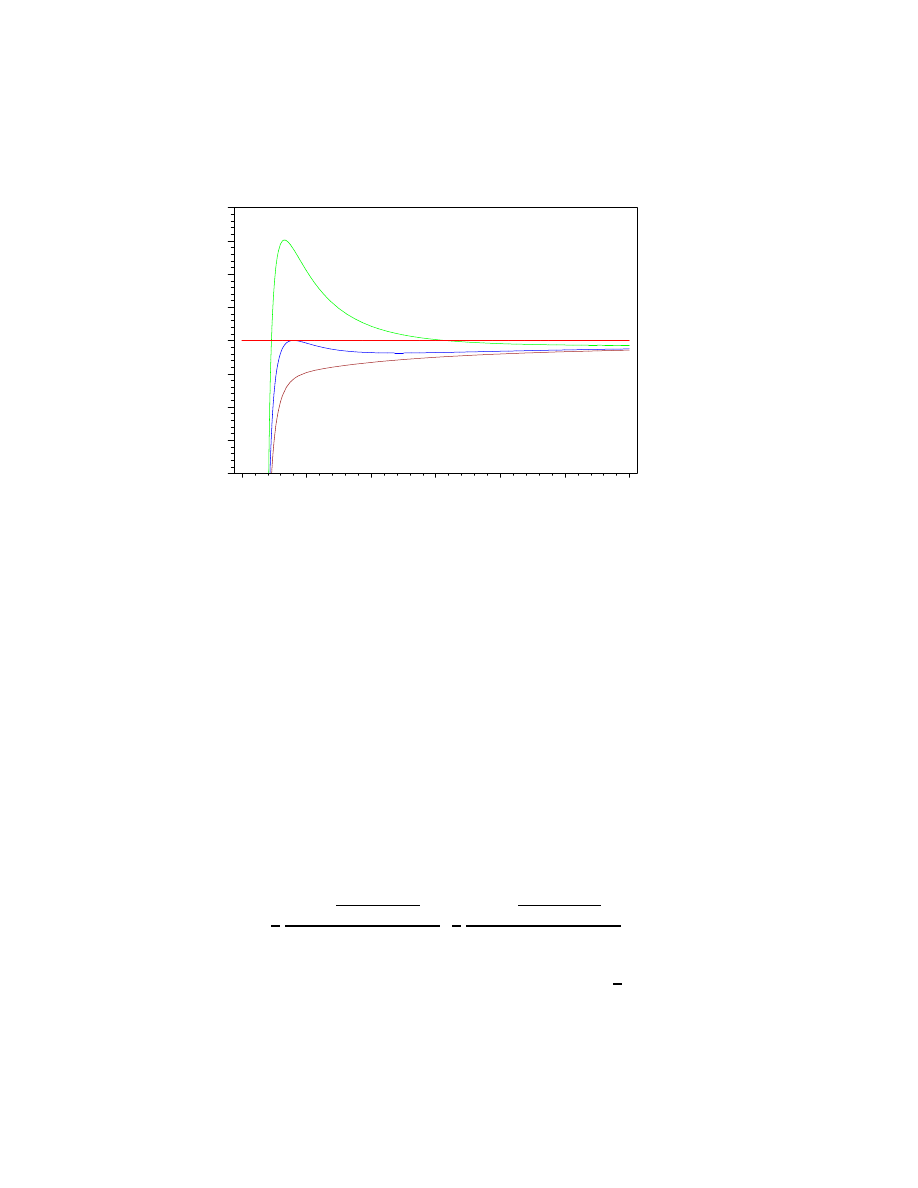
potentials
0.6
0.7
0.8
0.9
1
1.1
1.2
1.3
1.4
0
5
10
15
20
25
30
x
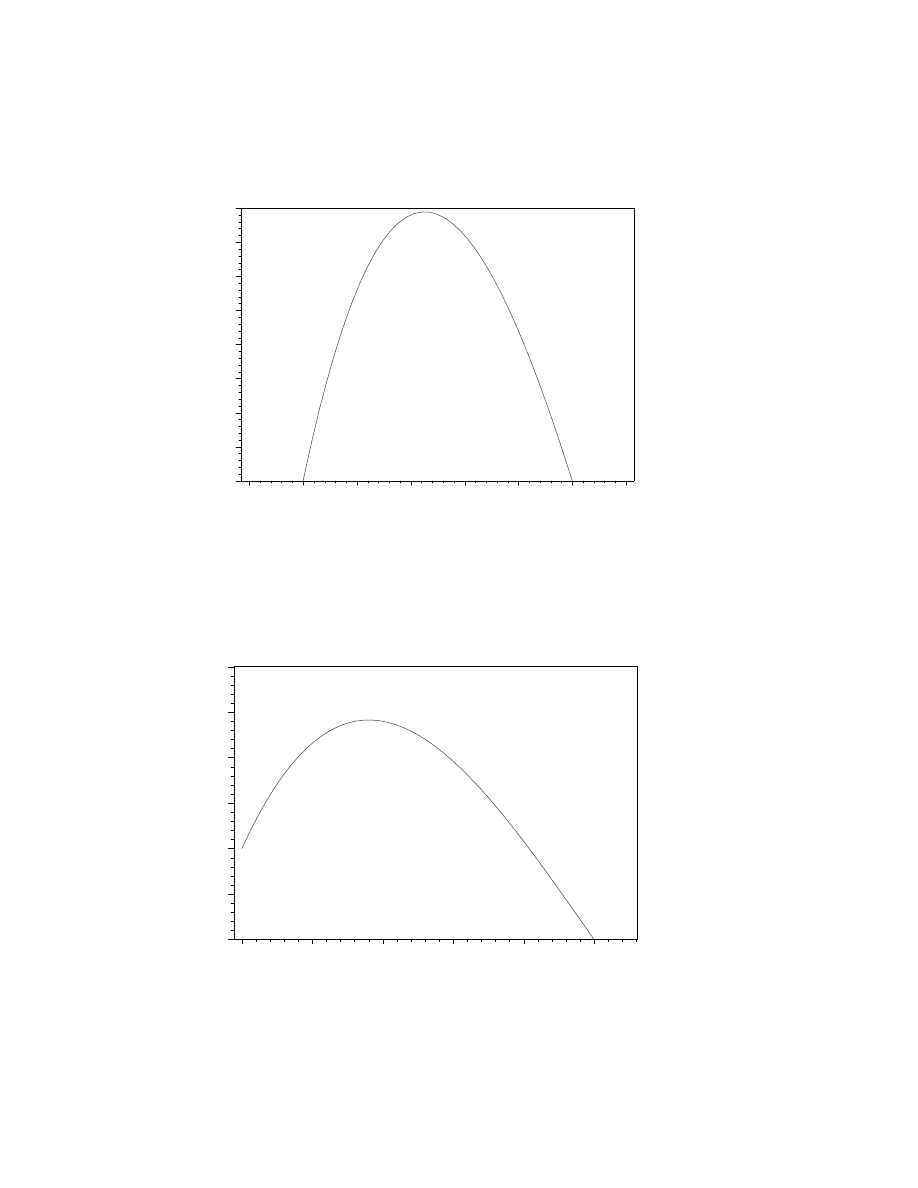
We considered the motion in the relativistic potential in the first part, but
only in the framework of linear approximation (weak field). As result of such
motion the perihelion rotation and light ray deflection appear. But now, in
the more general case, one can see a very interesting feature of the relativistic
orbital motion: unlike Newtonian case there is the maximum V
max
with the
following potential decrease as result of radial coordinate decrease. If V
max
>E > 1 the motion is infinite (it is analogue of the hyperbolical motion in
Newtonian case). V
max
>E =1 corresponds to parabolic motion. When E
lies in the potential hole or E = V, we have the finite motion. The motion
with energy, which is equal to extremal values of potential, corresponds to
circle orbits (the stable motion for potential minimum, unstable one for the
maximum). The existence of the extremes is defined by expressions:
>
numer( simplify( diff( subs(r(tau)=r,V), r) ) ) =\
>
0:# zeros of potential’s derivative
>
solve(%,r);
1
2
(L +
√
L
2
− 12 M
2
) L
M
,
1
2
(L
−
√
L
2
− 12 M
2
) L
M
As consequence, the circle motion is possible if L
≥ 2M
√
3 , when r
≥
3(2M ). The minimal distance, which allows the circular unstable motion, is
defined by
>
limit(1/2*(L-sqrt(L^2-12*M^2))*L/M, L=infinity);
38

3 M
Lack of extremes (red curve) or transition to r < 3M results in the falling
motion (the similar case is E > V
max
). This is the so-called gravitational
capture and has no analogy in Newtonian mechanics of point-like masses.
The finite orbital motion in the case of the right local minimum existence
(blue curve) is the analog of one in the Newtonian case, but has no elliptical
character (see first part).
As the particular case, let’s consider the radial (L=0) fall of particle. The
proper time of falling particle is defined by next expression
>
tau = Int(\ 1/sqrt(subs(
{L=0,r(tau)=r},rhs(eq6))),r);
>
tau = Int(1/(sqrt(2*M/r-2*M/R)),r);#R=2*M/(1-E^2) -\
>
apoastr, i.e.
radius of zero velocity
>
limit( value( rhs(%) ),r=2*M ):
>
simplify(%);#So, this is convergent integral\
>
for r-->2*M
τ =
Z
1
r
E
2
+
2 M
r
− 1
dr
τ =
Z
1
r
2
M
r
−
2 M
R
dr
1
4
r
−2 M + R
R
R(
−2
√
2
p
−(−2 M + R) M + R ln(2)
−R ln(−R + 4 M + 2
√
2
p
−(−2 M + R) M))
√
2
.p
−(−2 M + R) M
For the remote exterior observer we have
∂
∂τ
r =
∂
∂t
r
∂
∂τ
t =
∂
∂t
r
E
1
−
2 M
r
=
E
∂
∂t
r
o
(here r
0
is the time coordinate relatively infinitely remote observer):
>
r[o] := Int(1/(1-2*M/r),r) = int(1/(1-2*M/r),r);
>
limit( value( rhs(%) ),r=2*M );#this is\
>
divergent integral for r-->2*M
39
r
o
:=
Z
1
1
−
2 M
r
dr = r + 2 M ln(r
− 2 M)
−signum(M) ∞
These equations will be utilized below.
3.4
Degeneracy stars and gravitational collapse
The previously obtained expressions for the time of radial fall have an in-
teresting peculiarity if the radius of star is less or equal to 2M (
2 G M
c
2
in
dimensional case, that is the so-called ”gravitational radius” R
g
). The fi-
nite proper time τ of fall corresponds to the infinite ”remote” time r
o
, when
r–>2M. This means, that for the remote observer the fall does not finish
never. It results from the relativistic time’s slowing-down. The consequence
of this phenomena is the infinite red shift of ”falling” photons because of the
red shift in Schwarzschild metric is defined by the next frequencies relation:
ω
1
ω
2
=
∆ τ
2
∆ τ
1
=
r
g
0, 0
(r
2
)
g
0, 0
(r
1
)
=
q
1
−
2 M
r2
q
1
−
2 M
r1
(here ∆ τ are the proper time intervals
between light flash in different radial points). Simultaneously, the escape
velocity is equal to
q
2 G M
R
that is the velocity of light for sphere with R=
R
g
. So, we cannot receive any information from interior of black hole.
How can appear the object with the radius, which is less than R
g
? In the
beginning we consider the pressure free radial (i.e. angular part of metric is
equal to 0) collapse of dust sphere with mass M.
40
>
r := ’r’:
>
E := ’E’:
>
subs( r=r(t),get_compts(sch) ):
>
d(s)^2 =\
>
%[1,1]*d(t)^2 + %[2,2]*d(r)^2;#Schwarzschild metric
>
-d(tau)^2 = collect(\
>
subs( d(r)=diff(r(t),t)*d(t),rhs(%)),d(t));#tau is\
>
the proper time for the observer on the surface\
>
of sphere
>
%/d(tau)^2;
>
subs(
{d(t)=E/(1-2*M/r(t)),d(tau)=1},%);#we used \
>
d(t)/d(tau) = E/(1-2*M/r)
>
pot_1 :=\
>
factor( solve(%,(diff(r(t),t))^2) );#"potential"
d(s)
2
= (
−1 +
2 M
r(t)
) d(t)
2
+
d(r)
2
1
−
2 M
r(t)
−d(τ)
2
=
−1 +
2 M
r(t)
+
(
∂
∂t
r(t))
2
1
−
2 M
r(t)
d(t)
2
−1 =
−1 +
2 M
r(t)
+
(
∂
∂t
r(t))
2
1
−
2 M
r(t)
d(t)
2
d(τ )
2
−1 =
−1 +
2 M
r(t)
+
(
∂
∂t
r(t))
2
1
−
2 M
r(t)
E
2
(1
−
2 M
r(t)
)
2
pot 1 :=
(r(t)
− 2 M)
2
(
−r(t) + E
2
r(t) + 2 M )
E
2
r(t)
3
41
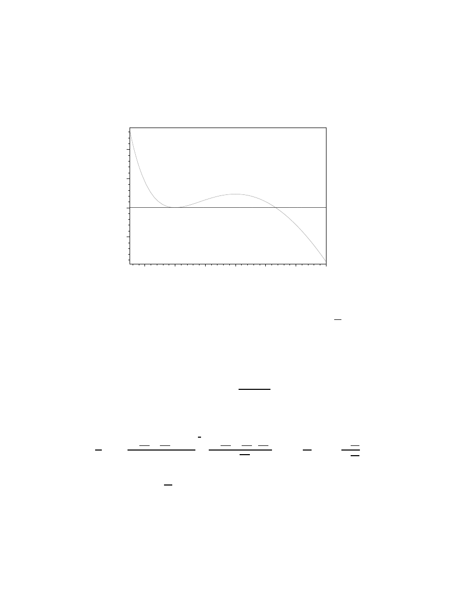
>
plot(
{subs({E=0.5,M=1,r(t)=r},pot_1),0*r},\
>
r=1.7..3,axes=boxed,title=‘(dr/dt)^2 vs r‘);
(dr/dt)^2 vs r
–0.02
0
0.02
0.04
1.8
2
2.2
2.4
2.6
2.8
3
r
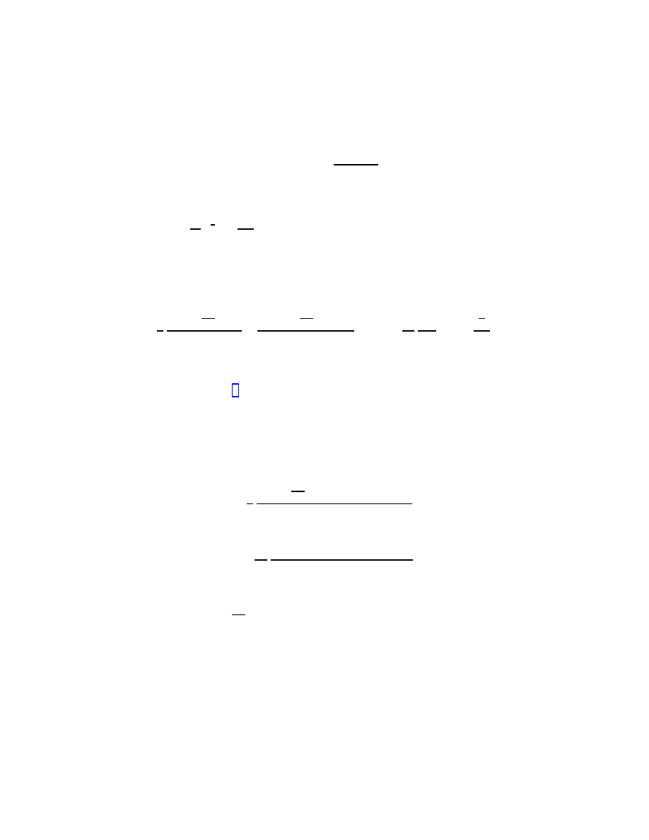
The collapse is the motion from the right point of zero velocity
∂
∂t
r (this
is the velocity for remote observer) to the left point of zero velocity. These
points are
>
solve(subs(r(t)=r,pot_1)=0,r);
2 M, 2 M,
−2
M
−1 + E
2
that are the apoastr (see above) and the gravitational radius. Hence (from
the value for apoastr and pot 1 )
(
∂
∂t
r)
2
=
(1
−
2 M
r
)
2
(
2 M
r
−1+E
2
)
E
2
=
(1
−
2 M
r
)
2
(
2 M
r
−
2 M
R
)
1
−
2 M
R
= (1
−
R
g
r
)
2
1
−
1
−
Rg
r
1
−
Rg
R
.
The slowing-down of the collapse for remote observer in vicinity of R
g
results
from the time slowing-down (see above). But the collapsing observer has
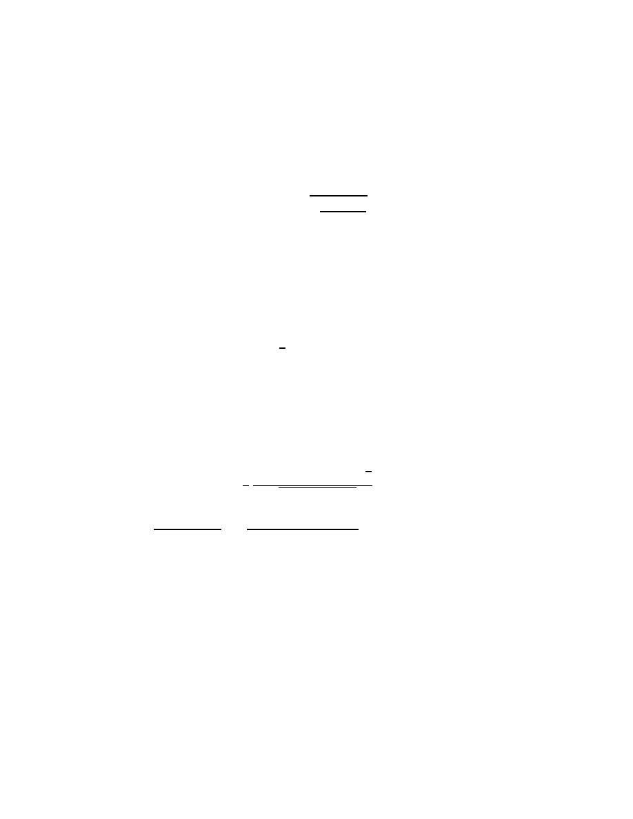
the proper velocity
∂
∂τ
r :
>
pot_2 := simplify(pot_1*(E/(1-2*M/r(t)))^2);#
>
d/d(t)=(d/d(tau))*(1-2*M/r)/E
42
pot 2 :=
−r(t) + E
2
r(t) + 2 M
r(t)
>
plot(
{subs({E=0.5,M=1,r(t)=r},pot_2),0*r},\
>
r=1.7..3,axes=boxed,title=‘(dr/dtau)^2 vs r‘);
(dr/dtau)^2 vs r
0
0.1
0.2
0.3
0.4
1.8
2
2.2
2.4
2.6
2.8
3
r
As result, the collapsing surface crosses the gravitational radius at finite
time moment and lim
r
→R
g
∂
∂t
r =1 (that is the velocity of light), when E =
1 (R=
∞ ). Time of collapse for falling observer is
>
Int(1/sqrt(R/r-1),r)/sqrt(1-E^2);#from pot_2,\
>
R is apoastr simplify( value(%), radical, symbolic);
Z
1
r
R
r
− 1
dr
√
1
− E
2
−
1
2
2
p
r (R
− r) + R arctan(
1
2
R
− 2 r
p
r (R
− r)
)
√
1
− E
2
It is obvious, that the obtained integral is
1
√
1
−E
2
R
R
r
1
p
R
r
−1
dr =
π R
√
1
−E
2
=
43

π M
(1
−E
2
)
( 3
2 )
.
It is natural, that the real stars are not clouds of dust and the equilibrium is
supported by nuclear reactions. But when the nuclear reactions in the star
finish, the ”fall” of the star’s surface can be prevented only by pressure of
electron or baryons. The equilibrium state corresponds to the minimum of
the net-energy composed of gravitational energy
−G M
2
R
and thermal kinetic
energy of composition. Let consider the hydrogen ball. When the temper-
ature tends to zero, the kinetic energy of electrons is not equal to zero due
to quantum degeneracy. In this case one electron occupies the cell with vol-
ume ˜ λ
3
, where λ =
h
2 π p
e
is the Compton wavelength ( p
e
is the electron’s
momentum). For non-relativistic electron:
>
E[e] := p[e]^2/m[e];#kinetic energy of electron
>
E[k] := simplify( n[e]*R^3*subs( p[e]=\
>
h*n[e]^(1/3)/(2*pi),E[e] ) );#full kinetic energy,\
>
n[e] is the number density of electrons
>
E[k] := subs( n[e]=M/R^3/m[p],%);# m[p] is the mass\
>
of proton.
We supposed m[e]<<m[p] and n[p]=n[e]
>
E[g] := -G*M^2/R:# gravitational energy
>
E := E[g] + E[k];# full energy
E
e
:=
p
e
2
m
e
E
k
:=
1
4
n
e
(5/3)
R
3
h
2
π
2
m
e
E
k
:=
1
4
(
M
R
3
m
p
)
(5/3)
R
3
h
2
π
2
m
e
E :=
−
G M
2
R
+
1
4
(
M
R
3
m
p
)
(5/3)
R
3
h
2
π
2
m
e
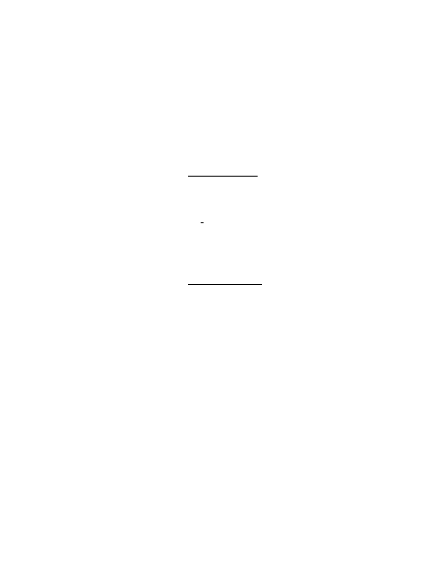
>
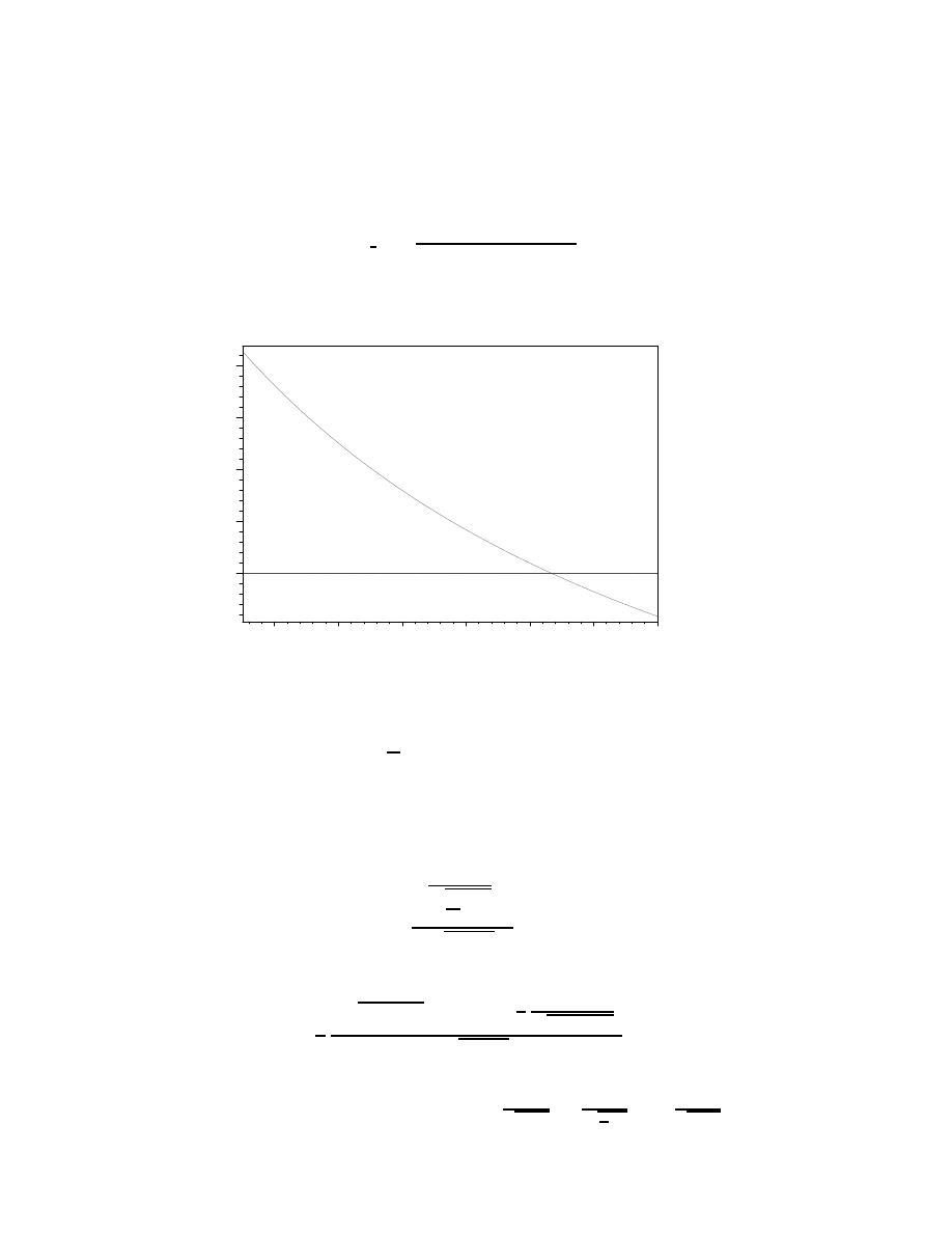
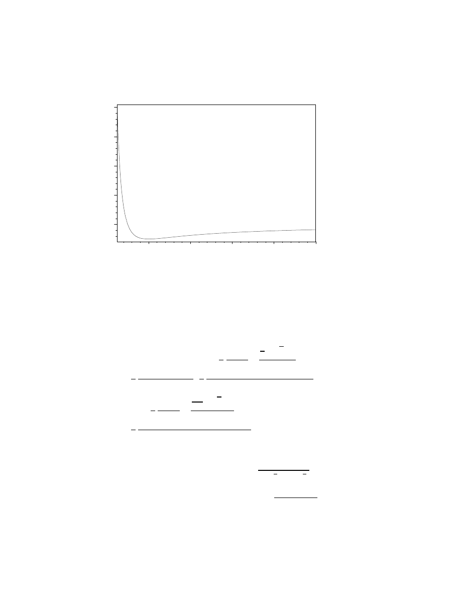
pot := -1/R+1/R^2:# the dependence of energy on R
>
plot(pot,R=0.5..10, \
>
title=‘energy of degenerated star‘);
44
energy of degenerated star
0
0.5
1
1.5
2
2
4
6
8
10
R
One can see that the dependence of energy on radius has the minimum and,
as consequence, there is the equilibrium state.
>
solve( diff(E, R) = 0, R);# minimum of energy\
>
corresponding to equilibrium state
1
2
%1 h
2
M m
p
2
π
2
m
e
G
,
1
2
−
1
2
%1
M m
p
+
1
2
I
√
3 %1
M m
p
h
2
π
2
m
p
m
e
G
,
1
2
−
1
2
%1
M m
p
+
−1
2
I
√
3 %1
M m
p
h
2
π
2
m
p
m
e
G
%1 := (M
2
m
p
)
(1/3)
So, we have the equilibrium state with R
min
˜
h
2
G M
( 1
3 )
m
e
m
p
( 5
3 )
and the star,
which exists in such equilibrium state as result of the termination of nuclear
reactions with the following radius decrease, is the white dwarf. The value
of number density in this state is
>
simplify( subs(\
>
R[min]=h^2/(G*M^(1/3)*m[e]*m[p]^(5/3)),\
>
n[e]=M/R[min]^3/m[p]));#equilibrium number density
45
n
e
=
M
2
G
3
m
e
3
m
p
4
h
6
So, the mass’s increase decreases the equilibrium radius (unlike model of
liquid drop, see above) and to increase the number density (the maximal
density of solid or liquid defined by atomic packing is ˜20 g/ cm
3
, for white
dwarf this value is ˜ 10
7
g/ cm
3
!). But, in compliance with principle of
uncertainty, the last causes the electron momentum increase ( p
e
n
e
(
−
1
3
)
˜
h). Our nonrelativistic approximation implies p
e
<< m
e
c or
>
simplify( rhs(%)^(1/3)*h ) - c*m[e];#this must be\
>
large negative value
>
solve(%=0,M);
(
M
2
G
3
m
e
3
m
p
4
h
6
)
(1/3)
h
− c m
e
√
G c h h c
G
2
m
p
2
,
−
√
G c h h c
G
2
m
p
2
The last result gives the nonrelativistic criterion M <<
(h c)
( 3
2
)
m
p
2
G
( 3
2
)
. Therefore
in the massive white dwarf the electrons have to be the relativistic particles:
>
E[e] := h*c*n[e]^(1/3);#E=p*c for relativistic particle
>
E[k] := simplify( n[e]*R^3*E[e] );
>
E[k] := subs( n[e]=M/R^3/m[p],%);
>
E[g] := -G*M^2/R:
>
E := E[g] + E[k];#this is dependence -a/R+b/R
>
#equilibrium state:
>
simplify( diff(E, R), radical ):
>
numer(%);#there is not dependence on R therefore\
>
there is not stable configuration with energy minimum
>
solve( %=0, M );
E
e
:= h c n
e
(1/3)
E
k
:= n
e
(4/3)
R
3
h c
46
E
k
:= (
M
R
3
m
p
)
(4/3)
R
3
h c
E :=
−
G M
2
R
+ (
M
R
3
m
p
)
(4/3)
R
3
h c
−(−G M m
p
+ (
M
R
3
m
p
)
(1/3)
h c R) M
0,
√
G c h h c
G
2
m
p
2
,
−
√
G c h h c
G
2
m
p
2
We obtained the estimation for so-called critical mass M
c
˜
(h c)
( 3
2 )
m
p
2
G
( 3
2 )
=1.4
M
sun
(so-called Chandrasekhar limit for white dwarfs). The smaller masses
produce the white dwarf with non-relativistic electrons but larger masses
causes collapse of star, which can not be prevented by pressure of degeneracy
electrons. Such collapse can form a neutron star for 1.4 M
sun
< M < 3 M
sun
.
Collapse for larger masses has to result in the black hole formation.
3.5
Schwarzschild black hole
Now we return to Schwarzschild metric.
>
get_compts(sch);
−1 +
2 M
r
0
0
0
0
1
1
−
2 M
r
0
0
0
0
r
2
0
0
0
0
r
2
sin(θ)
2
One can see two singularities: r =2M and r =0. What is a sense of first
singularity? When we cross the horizon, sh
1, 1
and sh
2, 2
(i.e. g
0, 0
and
47
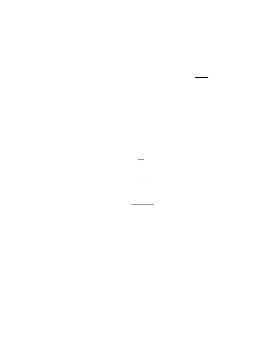
g
1, 1
) change signs. The space and time exchange the roles! The fall gets
inevitable as the time flowing. As consequence, when particle or signal cross
the gravitational radius, they cannot escape the falling on r =0. This fact
can be illustrated by infinite value of acceleration on r=2M, which is -
(Γ
α
)
0, 0
g
0, 0
( Γ are the Christoffel symbols):
>
D1sch := d1metric( sch, coord ):
>
Cf1 := Christoffel1 ( D1sch ):
>
displayGR(Christoffel1,%);
The Christoffel Symbols of the First Kind
non
− zero components :
[11 , 2 ] =
M
r
2
[12 , 1 ] =
−
M
r
2
[22 , 2 ] =
−
M
(r
− 2 M)
2
[23 , 3 ] = r
[24 , 4 ] = r sin(θ)
2
[33 , 2 ] =
−r
[34 , 4 ] = r
2
sin(θ) cos(θ)
[44 , 2 ] =
−r sin(θ)
2
48

[44 , 3 ] =
−r
2
sin(θ) cos(θ)
>
-get_compts(Cf1)[1,1,2]/get_compts(sch)[1,1];#radial\
>
component of acceleration
−
M
r
2
(
−1 +
2 M
r
)
Such particles and signals will be expelled from the cause-effect chain of
universe. Therefore an imaginary surface r = R
g
is named ”event horizon”.
The absence of true physical singularity for r = R
g
can be illustrated in the
following way. The invariant of Riemann tensor R
α, β, γ, δ
R
(α, β, γ, δ)
is
>
schinv := invert( sch, ’detg’ ):
>
D2sch := d2metric( D1sch, coord ):
>
Cf1 := Christoffel1 ( D1sch ):
>
RMN := Riemann( schinv, D2sch, Cf1 ):
>
raise(schinv,RMN,1):#raise of indexes\
>
in Riemann tensor
>
raise(schinv,%,2):
>
raise(schinv,%,3):
>
RMNinv := raise(schinv,%,4):
>
prod(RMN,RMNinv,[1,1],[2,2],[3,3],[4,4]);
table([compts = 48
M
2
r
6
, index char = []])
and has no singularity on horizon. This is only coordinate singularity and
its sense is the lack of rigid coordinates inside horizon. True physical sin-
gularity is r =0 and has the character of the so-called space-like singularity
(the inavitable singularity for the observer crossing horizon).
Now try to embed the instant equator section of curved space into flat space
(see above):
>
z(r)[1] = int(sqrt(2*r*M-4*M^2)/(-r+2*M),r);
>
z(r)[2] = int(-sqrt(2*r*M-4*M^2)/(-r+2*M),r);
z(r)
1
=
−2
p
2 r M
− 4 M
2
49
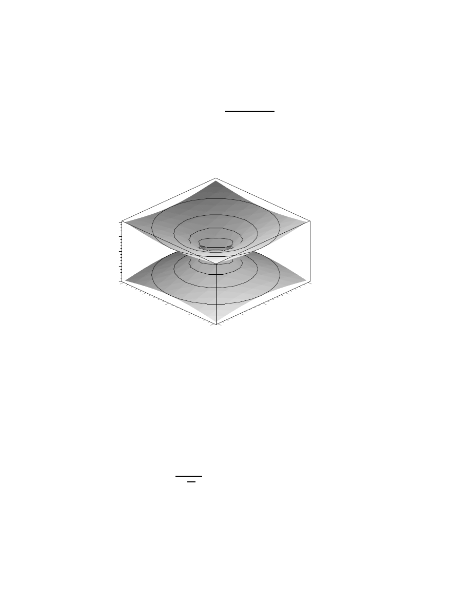
z(r)
2
= 2
p
2 r M
− 4 M
2
>
plot3d(
{subs({M=1,r=sqrt(x^2+y^2)},rhs(%%)),\
>
subs(
{M=1,r=sqrt(x^2+y^2)},rhs(%))},\
>
x=-10..10,y=-10..10,axes=boxed,style=PATCHCONTOUR,\
>
grid=[100,100],title=‘Schwarzschild black hole‘);
Schwarzschild black hole
–10
–5
0
5
10
x
–10
–5
0
5
10
y
–10
–5
0
5
10
This is the black hole, which looks as a neck of battle (Einstein-Rosen
bridge): the inside way to horizon and the outside way to horizon are the
ways between different but identically asymptotically flat universes (”worm-
hole” through 2-dimensional sphere with minimal radius 2M ). But since the
static geometry is not valid upon horizon (note, that here t–>t+dt is not
time translation), this scheme is not stable.
Let’s try to exclude the above-mentioned coordinate singularity on the hori-
zon by means of coordinate change. For example, we consider the null
geodesics ( ds
2
=0) in Schwarzschild space-time corresponding to radial mo-
tion of photons: dt
2
=
dr
2
(1
−
Rg
r
)
2
. Hence (see above considered expression for
r
0
):
>
t = combine( int(-1/(1-R[g]/r),r) );
t =
−r − R
g
ln(r
− R
g
)
50
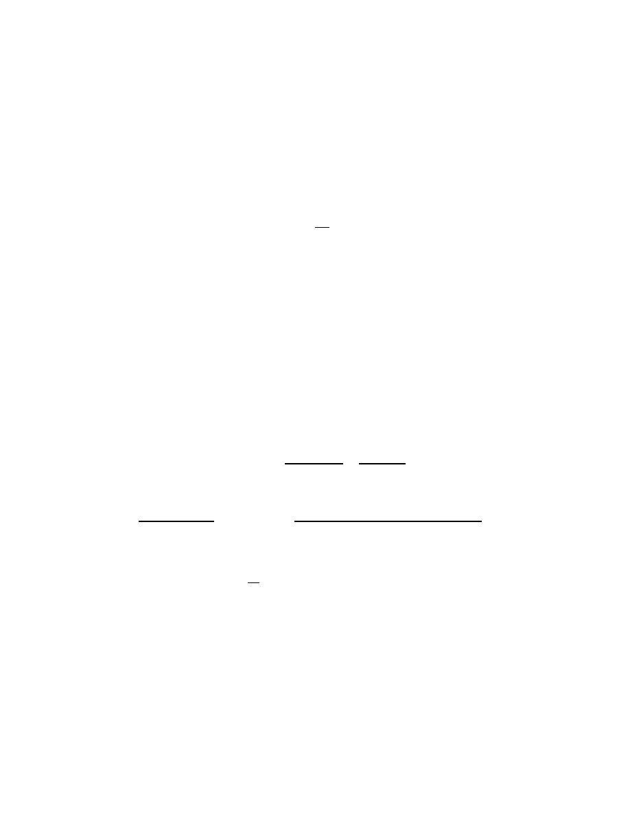
Then if v is the constant, which defines the radial coordinate for fixed t, we
have
>
t = -r - R[g]*ln( abs(-r/R[g]+1) ) + v;#module\
>
allows to extend the expression for r<R[g]
t =
−r − R
g
ln(
r
R
g
− 1
) + v
Differentiation of this equation with subsequent substitution of dt
2
in ex-
pression for interval in Schwarzschild metric produce
>
defform(f=0,w1=1,w2=1,w3=1,v=1,R[g]=0,r=0,v=0);
>
d(t)^2 = expand(\
>
subs( d(R[g])=0,\
>
d( -r-R[g]*ln( r/R[g]-1 )+v ) )^2);# differentials\
>
in new coordinates
>
subs( d(t)^2=rhs(%),sch_compts[1,1]*d(t)^2 ) +\
>
sch_compts[2,2]*d(r)^2 + sch_compts[3,3]*d(theta)^2 +\
>
sch_compts[4,4]*d(phi)^2:
>
collect( simplify( subs(R[g]=2*M,%) ),\
>
{d(r)^2,d(v)^2});#new metric
d(t)
2
= d(v)
2
−
2 d(v) r d(r)
r
− R
g
+
r
2
d(r)
2
(r
− R
g
)
2
−
(r
− 2 M) d(v)
2
r
+ 2 d(r) d(v)
−
−r
3
d(θ)
2
− r
3
d(φ)
2
+ r
3
d(φ)
2
cos(θ)
2
r
So, we have a new linear element (in the so-called Eddington - Finkelstein
coordinates) ds
2
= - ( 1
−
R
g
r
) dV
2
+ 2dvdr + r
2
d(Ω)
2
( d(Ω) is the spher-
ical part). The corresponding metric has the regular character in all region
of r (except for r =0). It should be noted, that the regularization was made
by transition to ”light coordinate” v therefore such coordinates can not be
realized physically, but formally we continued analytically the coordinates
to all r >0. We can see, that for future directed (i.e. dv
2
>0) null ( ds
2
=0) or time like ( ds
2
<0) worldlines dr <0 for r < R
g
that corresponds to
above-mentioned conclusion about inevitable fall on singularity.
In the conclusion, we consider the problem of the deviation from spher-
ical symmetry for static black hole. Such deviation can be described by
the characteristic of quadrupole momentum q. Erez and Rosen found the
51

corresponding static metric with axial symmetry:
>
coord := [t, lambda, mu, phi]:
>
er_compts :=\
>
array(symmetric,sparse,1..4,1..4):# metric components
>
er_compts[1,1] :=\
>
-exp(2*psi):# coefficient of d(t)^2 in interval
>
er_compts[2,2] :=\
>
M^2*exp(2*gamma-2*psi)*(lambda^2-mu^2)/\
>
(lambda^2-1):# coefficient of d(lambda)^2 in interval
>
er_compts[3,3] :=\
>
M^2*exp(2*gamma-2*psi)*(lambda^2-mu^2)/\
>
(1-mu^2):# coefficient of d(mu)^2 in interval
>
er_compts[4,4] :=\
>
M^2*exp(-2*psi)*(lambda^2-1)*(1-mu^2):#coefficient\
>
of d(phi)^2 in interval
>
er := create([-1,-1], eval(er_compts));# axially\
>
symmetric metric
er := table([compts =
−e
(2 ψ)
0
0
0
0
M
2
e
(2 γ
−2 ψ)
(λ
2
− µ
2
)
λ
2
− 1
0
0
0
0
M
2
e
(2 γ
−2 ψ)
(λ
2
− µ
2
)
1
− µ
2
0
0
0
0
M
2
e
(
−2 ψ)
(λ
2
− 1) (1 − µ
2
)
, index char = [
−1, −1]
])
where
>
f1 := psi = 1/2*(
>
(1+q*(3*lambda^2-1)*(3*mu^2-1)/4)*ln((lambda-1)/\
>
(lambda+1))+3/2*q*lambda*(3*mu^2-1) );
>
f2 := gamma =\
>
1/2*(1+q+q^2)*ln((lambda^2-1)/(lambda^2-mu^2))\
>
-3/2*q*(1-mu^2)*(lambda*ln((lambda-1)/(lambda+1))+2)\
>
+9/4*q^2*(1-mu^2)*((lambda^2+mu^2-1-9*lambda^2*mu^2)*\
>
(lambda^2-1)/16*ln((lambda-1)/(lambda+1))^2+\
>
(lambda^2+7*mu^2-5/3-9*mu^2*lambda^2)*lambda*\
>
ln((lambda-1)/(lambda+1))/4+1/4*lambda^2*(1-9*mu^2)+\
>
(mu^2-1/3) );
>
f3 := lambda = r/M-1;
>
f4 := mu = cos(theta);
f1 :=
ψ =
1
2
(1 +
1
4
q (3 λ
2
− 1) (3 µ
2
− 1)) ln(
λ
− 1
λ + 1
) +
3
4
q λ (3 µ
2
− 1)
52

f2 := γ =
1
2
(1 + q + q
2
) ln(
λ
2
− 1
λ
2
− µ
2
)
−
3
2
q (1
− µ
2
) (λ ln(
λ
− 1
λ + 1
) + 2) +
9
4
q
2
(1
− µ
2
)(
1
16
(λ
2
+ µ
2
− 1 − 9 λ
2
µ
2
) (λ
2
− 1) ln(
λ
− 1
λ + 1
)
2
+
1
4
(λ
2
+ 7 µ
2
−
5
3
− 9 λ
2
µ
2
) λ ln(
λ
− 1
λ + 1
)+
1
4
λ
2
(1
− 9 µ
2
) + µ
2
−
1
3
)
f3 := λ =
r
M
− 1
f4 := µ = cos(θ)
In the case q=0 we have
>
get_compts(er):
>
map2(subs,
{psi=rhs(f1),gamma=rhs(f2)},%):
>
map2(subs,q=0,%):
>
map2(subs,
{lambda=rhs(f3),mu=rhs(f4)},%):
>
map(simplify,%);
−
r
− 2 M
r
0
0
0
0
r M
2
r
− 2 M
0
0
0
0
−
r
2
−1 + cos(θ)
2
0
0
0
0
−r
2
(
−1 + cos(θ)
2
)
That is the Schwarzschild metric with regard to f3 and f4.
Now let’s find the horizon in the general case of nonzero quadrupole moment.
For static field (
∂
∂t
g
α, β
=0) the corresponding condition is g
0, 0
=0. Then
>
map2(subs,psi=rhs(f1),er):
>
er2 := map2(subs,gamma=rhs(f2),%):
>
get_compts(er2)[1,1];
53

−e
((1+1/4 q (3 λ
2
−1) (3 µ
2
−1)) ln(
λ
−1
λ+1
)+3/2 q λ (3 µ
2
−1))
That is r =2M ( λ =1). But the result for invariant of curvature is:
>
erinv := invert( er2, ’detg’ ):
>
D1er := d1metric( er2, coord ):
>
D2er := d2metric( D1er, coord ):
>
Cf1 := Christoffel1 ( D1er ):
>
RMN := Riemann( erinv, D2er, Cf1 ):
>
raise(erinv,RMN,1):#raise of indexes\
>
in Riemann tensor
>
raise(erinv,%,2):
>
raise(erinv,%,3):
>
RMNinv := raise(erinv,%,4):
>
prod(RMN,RMNinv,[1,1],[2,2],[3,3],[4,4]):
>
get_compts(%):
>
series(%,q=0,2):#expansion on q
>
convert(%,polynom):
>
res := simplify(%):
In the spherical case the result corresponds to above obtained:
>
factor( subs(q=0,res) ):#spherical symmetry
>
subs(lambda=1,%);# this is 48*M^2/r^6
3
4
1
M
4
There is no singularity. But for nonzero q (let’s choose µ = 0 for sake of
simplification):
>
subs(mu=0,res):
>
#L’Hospital’s rule for calculation of limit
>
limit(diff(numer(%),lambda),lambda=1);
>
limit(diff(denom(%),lambda),lambda=1);
−signum(q) ∞
0
Hence, there is a true singularity on horizon that can be regarded as the
54

demonstration of the impossibility of static axially symmetric black hole
with nonzero quadrupole momentum. Such momentum will be ”taken away”
by the gravitational waves in the process of the black hole formation.
3.6
Reissner-Nordstr¨
om black hole (charged black hole)
The generalization of Schwarzschild metric on the case of spherically sym-
metric vacuum solution of bounded Einstein-Maxwell equations results in
>
coord := [t, r, theta, phi]:
>
rn_compts := \
>
array(symmetric,sparse,1..4,1..4):# metric components
>
rn_compts[1,1] :=\
>
-(1-2*M/r+Q^2/r^2):# coefficient of d(t)^2 in interval
>
rn_compts[2,2] :=\
>
1/(1-2*M/r+Q^2/r^2):# coefficient of d(r)^2 in interval
>
rn_compts[3,3] := \
>
g_matrix[3,3]:# coefficient of d(theta)^2 in interval
>
rn_compts[4,4] :=\
>
g_matrix[4,4]:# coefficient of d(phi)^2 in interval
>
rn :=\
>
create([-1,-1], eval(rn_compts));# Reissner-Nordstrom\
>
(RN) metric
rn :=
table([compts =
−1 +
2 M
r
−
Q
2
r
2
0
0
0
0
1
1
−
2 M
r
+
Q
2
r
2
0
0
0
0
r
2
0
0
0
0
r
2
sin(θ)
2
,
index char = [
−1, −1]
])
Here Q is the electric charge. The metric has three singularities: r =0 and
>
denom(get_compts(rn)[2,2]) = 0;
>
r_p := solve(%, r)[1];
>
r_n := solve(%%, r)[2];
r
2
− 2 r M + Q
2
= 0
55

r p := M +
q
M
2
− Q
2
r n := M
−
q
M
2
− Q
2
Let’s calculate the invariant of curvature:
>
rninv := invert( rn, ’detg’ ):
>
D1rn := d1metric( rn, coord ):
>
D2rn := d2metric( D1rn, coord ):
>
Cf1 := Christoffel1 ( D1rn ):
>
RMN := Riemann( rninv, D2rn, Cf1 ):
>
raise(rninv,RMN,1):#raise of indexes\
>
in Riemann tensor
>
raise(rninv,%,2):
>
raise(rninv,%,3):
>
RMNinv := raise(rninv,%,4):
>
prod(RMN,RMNinv,[1,1],[2,2],[3,3],[4,4]);
table([compts = 8
6 r
2
M
2
− 12 r M Q
2
+ 7 Q
4
r
8
, index char = []])
>
solve(get_compts(%),r);#nonphysical roots for\
>
numerator with nonzero Q
(1 +
1
6
I
√
6) Q
2
M
,
(1
−
1
6
I
√
6) Q
2
M
That is the situation like to one in Schwarzschild metric and two last sin-
gularities have a coordinate character. Now let us plot the signs of two first
terms in linear element (we plot inverse value for second term in order to
escape the divergence due to coordinate singularities).
>
plot(
{subs({M=1,Q=1/2},get_compts(rn)[1,1]),\
>
subs(
{M=1,Q=1/2},1/get_compts(rn)[2,2])},\
>
r=0.1..2, title=‘signs of first and second terms of\
>
linear element‘);
56
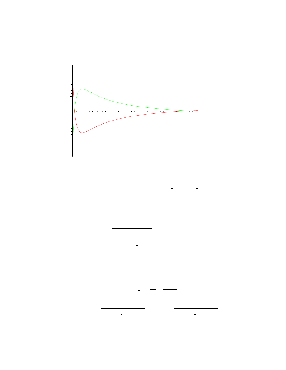
signs of first and second terms of linear element
–6
–4
–2
0
2
4
6
0.2 0.4 0.6 0.8
1
1.2 1.4 1.6 1.8
2
r
One can see the radical difference from the Schwarzschild black hole. The
space and time terms exchange the roles in region r n < r < r p (between
so-called inner and outer horizons with g
0, 0
=0). But there are the usual
signs in the vicinity of physical singularity, i. e. it has a time-like character
and the falling observer can avoid this singularity.
Next difference is the lack of coordinate singularities for M
2
< Q
2
. In this
case we have the so-called naked singularity. One can demonstrate that there
is no such singularity as result of usual collapse of charged shell with mass
M and charge Q. The total energy (in Newtonian limit but with correction
in framework of special relativity, M 0 is the rest mass) is
>
en := M(r) = M_0 + Q^2/r - M(r)^2/r;#we use\
>
the geometric units of charge so that the Coulomb low is\
>
G*Q_1*Q_2/r^2
>
sol := solve(en,M(r));
en := M(r) = M 0 +
Q
2
r
−
M(r)
2
r
sol :=
−
1
2
r +
1
2
q
r
2
+ 4 M 0 r + 4 Q
2
,
−
1
2
r
−
1
2
q
r
2
+ 4 M 0 r + 4 Q
2
The choice of the solution is defined by the correct asymptotic lim
r
→∞
sol
57
= M 0 :
>
if limit(sol[1],r=infinity)=M_0 then true_sol :=\
>
sol[1] fi:
>
if limit(sol[2],r=infinity)=M_0 then true_sol :=\
>
sol[2] fi:
>
true_sol;
−
1
2
r +
1
2
q
r
2
+ 4 M 0 r + 4 Q
2
>
diff(true_sol,r):
>
subs(M_0=solve(en,M_0),%):
>
simplify(%,radical,symbolic);
−Q
2
+ M(r)
2
(r + 2 M(r)) r
So,
∂
∂r
M(r) =
M(r)
2
−Q
2
r (r+2 M(r))
. The collapse is possible if M decreases with
decreasing R (domination of gravity over the Coulomb interaction in the
process of collapse) that is possible, when M
2
> Q
2
. It should be noted,
that the limit
>
limit(true_sol,r=0);
q
Q
2
resolves the problem of the infinite proper energy of charged particle.
Now we will consider the pressure free collapse of charged sphere of dust by
analogy with Schwarzschild metric.
58
>
r := ’r’:
>
E := ’E’:
>
subs( r=r(t),get_compts(rn) ):
>
d(s)^2 = %[1,1]*d(t)^2 + %[2,2]*d(r)^2;#RN metric
>
-d(tau)^2 =\
>
collect(subs( d(r)=diff(r(t),t)*d(t),\
>
rhs(%)),d(t));#tau is the proper time for the observer\
>
on the surface of sphere
>
%/d(tau)^2;
>
subs(
{d(t)=E/(1-2*M/r(t)+Q^2/r^2),\
>
d(tau)=1
},%);#we used d(t)/d(tau)=E/(1-2*M/r+Q^2/r^2)
>
pot_1 :=\
>
factor( solve(%,(diff(r(t),t))^2) ):#"potential"\
>
for remote observer
>
pot_2 :=\
>
simplify(pot_1*(E/(1-2*M/r(t)+Q^2/r^2))^2):#"potential"\
>
for collapsing observer\
>
d/d(t)=(d/d(tau))*(1-2*M/r+Q^2/r^2)/E
d(s)
2
= (
−1 +
2 M
r(t)
−
Q
2
r(t)
2
) d(t)
2
+
d(r)
2
1
−
2 M
r(t)
+
Q
2
r(t)
2
−d(τ)
2
=
−1 +
2 M
r(t)
−
Q
2
r(t)
2
+
(
∂
∂t
r(t))
2
1
−
2 M
r(t)
+
Q
2
r(t)
2
d(t)
2
−1 =
−1 +
2 M
r(t)
−
Q
2
r(t)
2
+
(
∂
∂t
r(t))
2
1
−
2 M
r(t)
+
Q
2
r(t)
2
d(t)
2
d(τ )
2
−1 =
−1 +
2 M
r(t)
−
Q
2
r(t)
2
+
(
∂
∂t
r(t))
2
1
−
2 M
r(t)
+
Q
2
r(t)
2
E
2
(1
−
2 M
r(t)
+
Q
2
r
2
)
2
59
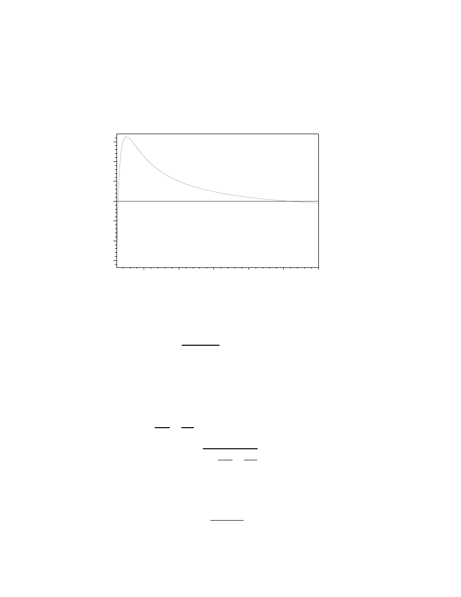
>
plot(
{subs({E=0.5,M=1,Q=1/2,r(t)=r},pot_2),\
>
0*r
},r=0.11..3,axes=boxed,title=‘(dr/dtau)^2 vs r for\
>
collapsing observer‘);
(dr/dtau)^2 vs r for collapsing observer
–3
–2
–1
0
1
2
3
0.5
1
1.5
2
2.5
3
r
The difference from Schwarzschild collapse is obvious: the observer crosses
the outer and inner horizons but does not reach the singularity because of
the collapsar explodes as white hole due to repulsion with consequent rec-
ollapse and so on.
And at last, we consider the ”extreme” case M
2
= Q
2
.
>
subs(Q^2=M^2, get_compts(rn));
>
factor(%[1,1]);
−1 +
2 M
r
−
M
2
r
2
0
0
0
0
1
1
−
2 M
r
+
M
2
r
2
0
0
0
0
r
2
0
0
0
0
r
2
sin(θ)
2
−
(r
− M)
2
r
2
60

So, we have one coordinate singularity in r =M. What happen with second
horizon? Let’s find the distance between horizons for fixed t and angular
coordinates for RN-metric:
>
get_compts(rn):
>
d(s)^2 = %[2,2]*d(r)^2;#RN metric
>
# or
>
d(s)^2 = d(r)^2/expand( (1-r_p/r)*(1-r_n/r) );#second\
>
representation of expression
d(s)
2
=
d(r)
2
1
−
2 M
r
+
Q
2
r
2
d(s)
2
=
d(r)
2
1
−
2 M
r
+
Q
2
r
2
Hence, when r p–>r n ( M
2
− Q
2
–>0)
>
r_p := ’r_p’:
>
r_n := ’r_n’:
>
s = Int(1/sqrt((1-r_p/r)*(1-r_n/r)),r=r_n..r_p) ;
>
simplify( value(rhs(%)),radical,symbolic );
s =
Z
r p
r n
1
r
(1
−
r p
r
) (1
−
r n
r
)
dr
1
2
r n ln(r p
− r n) +
1
2
r p ln(r p
− r n)−
1
2
r n ln(
−r p + r n) −
1
2
r p ln(
−r p + r n)
we have s–>
∞ . So, there is the infinitely long Einstein-Rosen bridge
(charged string) between horizons that means a lack of wormhole between
asymptotically flat universes. This fact can be illustrated by means of em-
bedding of equatorial section of static RN space in flat Euclidian space (see
above).
61
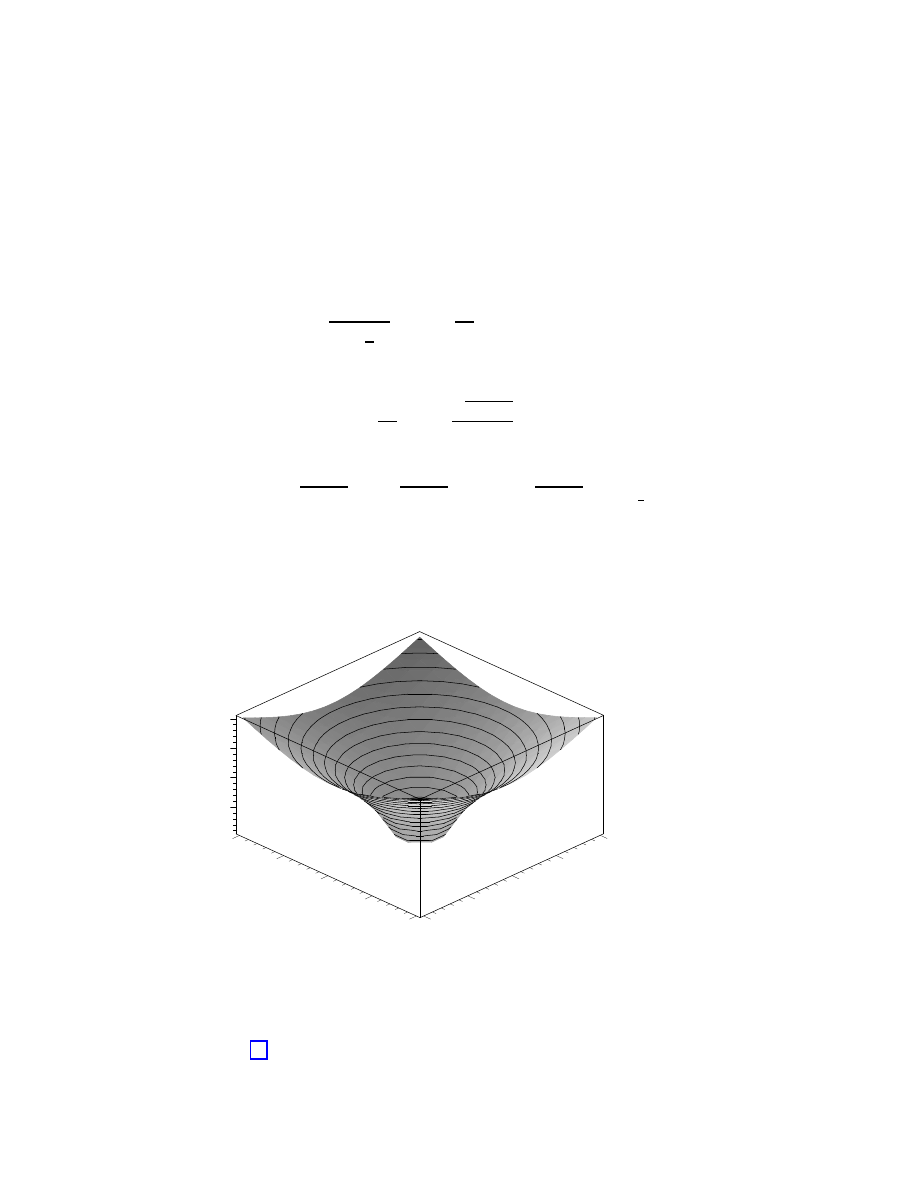
>
d(r)^2/(1-1/r)^2
=\
>
(1+diff(z(r),r)^2)*d(r)^2;#equality of radial elements\
>
of intervals, M=1
>
diff(z(r),r) = solve(%,diff(z(r),r))[1];
>
dsolve(%,z(r));# embedding
d(r)
2
(1
−
1
r
)
2
= (1 + (
∂
∂r
z(r))
2
) d(r)
2
∂
∂r
z(r) =
√
2 r
− 1
r
− 1
z(r) = 2
√
2 r
− 1 + ln(
√
2 r
− 1 − 1) − ln(
√
2 r
− 1 + 1) + C1
>
plot3d(subs(r=sqrt(x^2+y^2),\
>
2*sqrt(2*r-1)+ln(sqrt(2*r-1)-1)-ln(sqrt(2*r-1)+1)),\
>
x=-10..10,y=-10..10,axes=boxed,style=PATCHCONTOUR,\
>
grid=[100,100],title=‘extreme RN black hole‘);\
>
#we expressed arctanh through ln
extreme RN black hole
–10
–5
0
5
10
x
–10
–5
0
5
10
y
4
6
8
10
The asymptotic behavior of RN-metric as r–>
∞ is Minkowski. For inves-
tigation of the situation r–>M let introduce the new coordinate (see, for
example, [10]):
62

>
rn_assym := subs(\
>
{r=M*(1+lambda),Q^2=M^2},get_compts(rn) );
rn assym :=
−1 +
2
λ + 1
−
1
(λ + 1)
2
0
0
0
0
1
1
−
2
λ + 1
+
1
(λ + 1)
2
0
0
0
0
M
2
(λ + 1)
2
0
0
0
0
M
2
(λ + 1)
2
sin(θ)
2
>
m1 :=\
>
series(rn_assym[1,1],lambda=0,3);# we keep only\
>
leading term in lambda
>
m2 :=\
>
series(rn_assym[2,2],lambda=0,3);# we keep only\
>
leading term in lambda
>
d(s)^2 = convert(m1,polynom)*d(t)^2\
>
+ M^2*convert(m2,polynom)*d(lambda)^2 +\
>
M^2*d(Omega)^2;#d(Omega) is spherical part
m1 :=
−λ
2
+ O(λ
3
)
m2 := λ
−2
+ O(λ
−1
)
d(s)
2
=
−λ
2
d(t)
2
+
M
2
d(λ)
2
λ
2
+ M
2
d(Ω)
2
This is the Robinson-Bertotti metric. The last term describes two - dimen-
sional sphere with radius M (these dimensions are compactified in the vicin-
ity of horizon) and the first terms corresponds to anti-de Sitter space-time
(see below) with constant negative curvature.
3.7
Kerr black hole (rotating black hole)
In the general form the stationary rotating black hole is described by so-
called Kerr-Newman metric, which in the Boyer-Linquist coordinates can
be presented as:
63

>
coord := [t, r, theta, phi]:
>
kn_compts :=\
>
array(sparse,1..4,1..4):# metric components,\
>
a=J/M, J is the angular momentum
>
kn_compts[1,1] :=\
>
-(Delta-a^2*sin(theta)^2)/Sigma:#coefficient of d(t)^2
>
kn_compts[1,4] :=\
>
-2*a*sin(theta)^2*(r^2+a^2-Delta)/\
>
Sigma:# coefficient of d(t)*dphi
>
kn_compts[2,2] :=\
>
Sigma/Delta:# coefficient of d(r)^2
>
kn_compts[3,3] :=\
>
Sigma:# coefficient of d(theta)^2
>
kn_compts[4,4] :=\
>
(((r^2+a^2)^2-Delta*a^2*sin(theta)^2)/\
>
Sigma)*sin(theta)^2:#coefficient of d(phi)^2
>
kn := create([-1,-1], eval(kn_compts));# Kerr-Newman\
>
(KN) metric
>
#where
>
sub_1 := Sigma = r^2+a^2*cos(theta)^2;
>
sub_2 := Delta = r^2-2*M*r+a^2+sqrt(Q^2+P^2);# P is\
>
the magnetic (monopole) charge
kn := table([compts =
−
∆
− a
2
sin(θ)
2
Σ
0
0
−2
a sin(θ)
2
(r
2
+ a
2
− ∆)
Σ
0
Σ
∆
0
0
0
0
Σ
0
0
0
0
((r
2
+ a
2
)
2
− ∆ a
2
sin(θ)
2
) sin(θ)
2
Σ
,
index char = [
−1, −1]
])
sub 1 := Σ = r
2
+ a
2
cos(θ)
2
sub 2 := ∆ = r
2
− 2 r M + a
2
+
q
Q
2
+ P
2
In the absence of charges, this results in Kerr metric. The obvious singular-
ities are (except for an usual singularity of spherical coordinates θ =0):
64

>
r_p :=\
>
solve( subs(
{Q=0,P=0},\
>
rhs(sub_2))=0,r )[1];#outer horizon
>
r_n :=\
>
solve( subs(
{Q=0,P=0},\
>
rhs(sub_2))=0,r )[2];#inner horizon
>
solve( subs(
{Q=0,P=0},rhs(sub_1))=0,theta );
r p := M +
p
M
2
− a
2
r n := M
−
p
M
2
− a
2
1
2
π
− I arcsinh(
r
a
),
1
2
π + I arcsinh(
r
a
)
The last produces r =0, θ =
π
2
.
As it was in the case of charged static black hole, there are three different
situations: M
2
< a
2
, M
2
= a
2
, M
2
> a
2
.
Let us consider the signs of g
0, 0
, g
1, 1
, g
4, 4
( M
2
> a
2
).
>
plot3d(subs(
{M=1,a=1/2,P=0,Q=0},subs(\
>
{Sigma=rhs(sub_1),Delta=rhs(sub_2)},\
>
get_compts(kn)[1,1])),r=0.1..4,theta=0..Pi,color=red):
>
plot3d(subs(
{M=1,a=1/2,P=0,Q=0,theta=2*Pi/3},\
>
subs(
{Sigma=rhs(sub_1),Delta=rhs(sub_2)},\
>
1/get_compts(kn)[2,2])),\
>
r=0.1..4,theta=0..Pi,color=green):
>
display(%,%%,\
>
title=‘signs of first and second diagonal elements\
>
of metric‘,axes=boxed);
>
plot3d(subs(
{M=1,a=1/2,P=0,Q=0},subs(\
>
{Sigma=rhs(sub_1),Delta=rhs(sub_2)},\
>
get_compts(kn)[4,4])),r=-0.01..0.01,\
>
theta=Pi/2-0.01..Pi/2+0.01,color=blue,\
>
title=‘four diagonal element of metric in vicinity of\
>
singularity‘,axes=boxed);
65
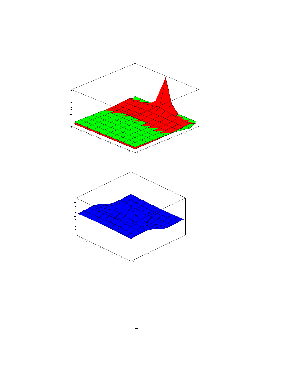
signs of first and second diagonal elements of metric
1
2
3
4
r
0
0.5
1
1.5
2
2.5
3
theta
0
5
10
15
four diagonal element of metric in vicinity of singularity
–0.01
–0.005
0
0.005
0.01
r
1.565
1.57
1.575
1.58
theta
–200
–100
0
100
200
One can see, that the approach to r =0 in the line, which differs from θ =
π
2
,
corresponds to usual signs of diagonal elements of metric, i.e. the observer
crosses r =0 and comes into region r <0 without collision with singularity.
But from the second picture we can see the change of the g
3, 3
-sign for r <0.
Now φ is the time like coordinate. But this coordinate has circle character
and, as consequence, we find oneself in the world with closed time lines. The
approach to r =0 in the line of θ =
π
2
produces the change of g
0, 0
-sign, i.e.
we find a true singularity in this direction. These facts demonstrate that
66

the singularity in Kerr black hole has a more complicated character than in
above considered black holes.
The more careful consideration gives the following results:
1) M
2
< a
2
. There exist no horizon (r p and r n are complex), but the
singularity in r =0, θ =
π
2
keeps. To remove the coordinate singularity in θ
=0 we introduce the Kerr-Schild coordinates with linear element
>
macro(ts=‘t*‘):
>
ks_le := d(s)^2 = -d(ts)^2 + d(x)^2 + d(y)^2\
>
+ d(z)^2 + (2*M*r^3/(r^4+a^2*z^2))*\
>
((r*(x*d(x)+y*d(y))-a*(x*d(y)-y*d(x)))/\
>
(r^2+a^2)+z*d(z)/r+d(ts) )^2;
>
x + I*y = (r + I*a)*sin(theta)*\
>
exp(I*(Int(1,phi)+Int(a/Delta,r)));
>
z = r*cos(theta);
>
ts = Int(1,t) + Int((r^2+a^2/Delta),r) - r;
ks le := d(s)
2
=
−d(t∗)
2
+ d(x)
2
+ d(y)
2
+ d(z)
2
+
2 M r
3
(
r (x d(x) + y d(y))
− a (x d(y) − y d(x))
r
2
+ a
2
+
z d(z)
r
+ d(t
∗))
2
r
4
+ a
2
z
2
x + I y = (r + I a) sin(θ) e(
I
(
R
1 dφ+
R
a
∆
dr
))
z = r cos(θ)
t
∗ =
Z
1 dt +
Z
r
2
+
a
2
∆
dr
− r
which is reduced to Minkowski metric by M–>0.
>
int(subs(
{P=0,Q=0},\
>
subs(Delta=rhs(sub_2),a/Delta) ),r):
>
x+I*y=(r+I*a)*sin(theta)*exp(I*(phi+%));
x + I y = (r + I a) sin(θ) e
I
φ+
a arctan(1/2 2 r−2 M
√
a2
−M 2
)
√
a2
−M 2
!!
When r =0, θ =
π
2
the singularity is the ring x
2
+ y
2
= a
2
, z = 0.
67

2) M
2
> a
2
. As before we have the ring singularity, but there are the
horizons r p and r n. As an additional feature of Kerr metric we note here
the existence of coordinate singularity:
>
get_compts(kn)[1,1]=0;
>
subs( Delta=rhs( sub_2 ),numer( lhs(%) ) ):
>
solve( subs(
{Q=0,P=0},%) = 0,r );
−
∆
− a
2
sin(θ)
2
Σ
= 0
M +
q
M
2
− a
2
+ a
2
sin(θ)
2
, M
−
q
M
2
− a
2
+ a
2
sin(θ)
2
The crossing of ellipsoid r 1 = M +
p
M
2
− a
2
cos(θ)
2
produces the change of
g
0, 0
-sign. As it was for Schwarzschild black hole this fact demonstrates the
lack of static coordinates under this surface, which is called ”ergosphere” and
the region between r p and r 1 is the ergoregion. The absence of singularity
for r
r, r
suggests that the nonstatic behavior results from entrainment of
observer by black hole rotation, but not from fall on singularity, as it takes
place for observer under horizon in Schwarzschild black hole.
3.8
Conclusion
So, the elementary analysis by means of basic Maple 6 functions allows to
obtain the main results of black hole physics including conditions of collapsar
formation, the space-time structure of static spherically symmetric charged
and uncharged black holes and stationary axially symmetric black hole.
4
Cosmological models
4.1
Introduction
I suppose that the most impressive achievements of the GR-theory belong
to the cosmology. The description of the global structure of the universe
changes our opinion about reality and radically widens the horizon of knowl-
edge. The considerable progress in the observations and measures allows to
say that we are living in a gold age of cosmology. Here we will consider some
68

basic conceptions of relativistic cosmology by means of analytical capabili-
ties of Maple 6.
4.2
Robertson-Walker metric
We will base on the conception of foliation of 4-dimensional manifold on
3-dimensional space-like hyperplanes with a time-dependent geometry. Now
let’s restrict oneself to the isotropic and homogeneous evolution models, i.e.
the models without dependence of curvature on the observer’s location or
orientation. We will suppose also, that such foliation with isotropic and ho-
mogeneous geometry and energy-momentum distribution exists at each time
moment. These space-like foliations are the so-called hyperplanes of homogeneity.
The time vectors are defined by the proper time course in each space point.
Let us consider 3-geometry at fixed time moment. As it is known, in 3-
dimensional space the curvature tensor has the following form:
R
iklm
=
R
il
g
km
- R
im
g
kl
+ R
km
g
il
- R
kl
g
im
+
R
2
( g
im
g
kl
- g
il
g
km
).
But if (as it takes a place in our case) there is not the dependence of curvature
on space-direction in arbitrary point, our space has a constant curvature
(Schur’s theorem) that results in
R
iklm
=
R
2
( g
im
g
kl
- g
il
g
km
), (1)
where R is the constant Ricci scalar.
Now we will consider the so-called Robertson-Walker metric:
g
ij
=
δ
ij
(1+
R δij xi xj
8
)
2
(2)
For this metric the spatial curvature tensor is:
69

>
restart:
>
with(tensor):
>
with(linalg):
>
with(difforms):
>
coord := [x, y, z]:# coordinates
>
g_compts :=\
>
array(symmetric,sparse,1..3,1..3):# metric components
>
g_compts[1,1] := 1/\
>
(1+R*(x^2+y^2+z^2)/8)^2:# component of interval\
>
attached to d(x)^2
>
g_compts[2,2] :=\
>
1/(1+R*(x^2+y^2+z^2)/8)^2:# component of interval\
>
attached to d(y)^2
>
g_compts[3,3] :=\
>
1/(1+R*(x^2+y^2+z^2)/8)^2:# component of\
>
interval attached to d(z)^2
>
g := create([-1,-1], eval(g_compts));# covariant\
>
metric tensor
>
ginv := invert( g, ’detg’ ):# contravariant\
>
metric tensor
>
D1g := d1metric( g, coord ):# calculation of \
>
curvature tensor
>
D2g := d2metric( D1g, coord ):
>
Cf1 := Christoffel1 ( D1g ):
>
RMN := Riemann( ginv, D2g, Cf1 ):
>
displayGR(Riemann, RMN);
g := table([index char = [
−1, −1], compts =
%1
0
0
0
%1
0
0
0
%1
])
%1 :=
1
(1 +
1
8
R (x
2
+ y
2
+ z
2
))
2
The Riemann Tensor
non
− zero components :
R1212 = 2048
R
(8 + R x
2
+ R y
2
+ R z
2
)
4
R1313 = 2048
R
(8 + R x
2
+ R y
2
+ R z
2
)
4
70

R2323 = 2048
R
(8 + R x
2
+ R y
2
+ R z
2
)
4
character : [
−1 , −1 , −1 , −1 ]
Now we try to perform the direct calculations from Eq. (1):
>
A := get_compts(g):
>
B := array(1..3, 1..3, 1..3, 1..3):
>
for i from 1 to 3 do
>
for j from 1 to 3 do
>
for k from 1 to 3 do
>
for l from 1 to 3 do
>
B[i,j,k,l] :=\
>
eval(R*(A[i,k]*A[j,l] - A[i,l]*A[j,k])/2):# Eq.
1.\
>
These calculations can be performed also by means of\
>
tensor[prod] and tensor[permute_indices]
>
if B[i,j,k,l]<>0 then \
>
print([i,j,k,l],B[i,j,k,l]);# non-zero components
>
else
>
fi:
>
od:
od:
od:
od:
[1, 2, 1, 2],
1
2
R
(1 +
1
8
R (x
2
+ y
2
+ z
2
))
4
[1, 2, 2, 1],
−
1
2
R
(1 +
1
8
R (x
2
+ y
2
+ z
2
))
4
[1, 3, 1, 3],
1
2
R
(1 +
1
8
R (x
2
+ y
2
+ z
2
))
4
[1, 3, 3, 1],
−
1
2
R
(1 +
1
8
R (x
2
+ y
2
+ z
2
))
4
71
[2, 1, 1, 2],
−
1
2
R
(1 +
1
8
R (x
2
+ y
2
+ z
2
))
4
[2, 1, 2, 1],
1
2
R
(1 +
1
8
R (x
2
+ y
2
+ z
2
))
4
[2, 3, 2, 3],
1
2
R
(1 +
1
8
R (x
2
+ y
2
+ z
2
))
4
[2, 3, 3, 2],
−
1
2
R
(1 +
1
8
R (x
2
+ y
2
+ z
2
))
4
[3, 1, 1, 3],
−
1
2
R
(1 +
1
8
R (x
2
+ y
2
+ z
2
))
4
[3, 1, 3, 1],
1
2
R
(1 +
1
8
R (x
2
+ y
2
+ z
2
))
4
[3, 2, 2, 3],
−
1
2
R
(1 +
1
8
R (x
2
+ y
2
+ z
2
))
4
[3, 2, 3, 2],
1
2
R
(1 +
1
8
R (x
2
+ y
2
+ z
2
))
4
The direct calculation on the basis of Eq. (1) and metric (2) results in the
tensor with symmetries [i,j,k,l ] = [k,l,i,j ] = [j,i,k,l ] = -[ i,j,l,k ] and [i,j,k,l ] +
[i,l,j,k ] + [i,k,l,j ] = 0. These symmetries and values of nonzero components
correspond to curvature tensor, which was calculated previously from (2). As
72

consequence, metric (2) satisfies to condition of constant curvature (Schur’s
theorem, Eq. (1)). We will base our further calculations on this metric.
The next step is the choice of the appropriate coordinates. We consider two
types of coordinates: spherical and pseudospherical.
In the case of the spherical coordinates the transition of Eq. (2) to a new
basis results in:
>
g_sp :=\
>
simplify(subs(\
>
{x=r*cos(phi)*sin(theta),y=r*sin(phi)*sin(theta),\
>
z=r*cos(theta)
},get_compts(g))):# This is transformation\
>
of coordinates in metric tensor
>
Sp_compts := array(1..3,1..3):# matrix of\
>
conversion from (NB!) spherical coordinates
>
Sp_compts[1,1] := cos(phi)*sin(theta):
>
Sp_compts[2,1] := sin(phi)*sin(theta):
>
Sp_compts[3,1] := cos(theta):
>
Sp_compts[1,2] := r*cos(phi)*cos(theta):
>
Sp_compts[2,2] := r*sin(phi)*cos(theta):
>
Sp_compts[3,2] := -r*sin(theta):
>
Sp_compts[1,3] := -r*sin(phi)*sin(theta):
>
Sp_compts[2,3] := r*cos(phi)*sin(theta):
>
Sp_compts[3,3] := 0:
>
Sp := eval(Sp_compts):
>
simplify(\
>
multiply(transpose(Sp), g_sp, Sp));#transition\
>
to new coordinates in metric
64
1
%1
0
0
0
64
r
2
%1
0
0
0
−64
r
2
(
−1 + cos(θ)
2
)
%1
%1 := (8 + R r
2
cos(φ)
2
sin(θ)
2
+ R r
2
sin(φ)
2
sin(θ)
2
+ R r
2
cos(θ)
2
)
2
The denominator is
>
denom(%[1,1]):
>
expand(%):
>
simplify(%,trig):
>
factor(%);
(R r
2
+ 8)
2
73
After substitution r* = r
q
R
2
(we will omit asterix and suppose R > 0),
the metric is converted as:
>
coord := [r, theta, phi]:# spherical coordinates
>
g_compts_sp :=\
>
array(symmetric,sparse,1..3,1..3):# metric components
>
g_compts_sp[1,1] :=\
>
(2/R)/(1+r^2/4)^2:# component of interval\
>
attached to d(r)^2
>
g_compts_sp[2,2] :=\
>
(2/R)*r^2/(1+r^2/4)^2:# component of interval\
>
attached to d(theta)^2
>
g_compts_sp[3,3] :=\
>
(2/R)*r^2*sin(theta)^2/(1+r^2/4)^2:# component of\
>
interval attached to d(phi)^2
>
g_sp := create([-1,-1], eval(g_compts_sp));# covariant\
>
metric tensor
g sp := table([index char = [
−1, −1],
compts =
2
1
R (1 +
1
4
r
2
)
2
0
0
0
2
r
2
R (1 +
1
4
r
2
)
2
0
0
0
2
r
2
sin(θ)
2
R (1 +
1
4
r
2
)
2
])
The denominator’s form suggests the transformation of radial coordinate:
sin( χ ) = r/ (1 + r
2
/4). Then for dr
2
-component we have
>
diff(sin(chi),chi)*d(chi) =\
>
simplify(diff(r/(1+r^2/4),r))*d(r);
>
lhs(%)^2 = rhs(%)^2;
>
subs(cos(chi)^2=1-r^2/(1+r^2/4)^2,lhs(%))\
>
= rhs(%):
>
factor(%);
cos(χ) d(χ) =
−4
(
−4 + r
2
) d(r)
(4 + r
2
)
2
cos(χ)
2
d(χ)
2
= 16
(
−4 + r
2
)
2
d(r)
2
(4 + r
2
)
4
74

(r
− 2)
2
(r + 2)
2
d(χ)
2
(4 + r
2
)
2
= 16
(r
− 2)
2
(r + 2)
2
d(r)
2
(4 + r
2
)
4
that leads to a new metric (d χ =
dr
(1+
r2
4
)
2
):
>
coord := [r, theta, phi]:# spherical coordinates
>
g_compts_sp :=\
>
array(symmetric,sparse,1..3,1..3):# metric components
>
g_compts_sp[1,1] := \
>
2/R:# component of interval attached to d(chi)^2
>
g_compts_sp[2,2] :=\
>
(2/R)*sin(chi)^2:# component of interval\
>
attached to d(theta)^2
>
g_compts_sp[3,3] :=\
>
(2/R)*sin(chi)^2*sin(theta)^2:# component of\
>
interval attached to d(phi)^2
>
g_sp :=\
>
create([-1,-1], eval(g_compts_sp));# covariant\
>
metric tensor
g sp := table([index char = [
−1, −1], compts =
2
1
R
0
0
0
2
sin(χ)
2
R
0
0
0
2
sin(χ)
2
sin(θ)
2
R
])
Here R/2 is the Gaussian curvature K (K >0) so that the linear element is:
>
l_sp := d(s)^2 = a^2*(d(chi)^2 +\
>
sin(chi)^2*(d(theta)^2+sin(theta)^2*d(phi)^2));
l sp := d(s)
2
= a
2
(d(χ)
2
+ sin(χ)
2
(d(θ)
2
+ sin(θ)
2
d(φ)
2
))
Here a =
q
1
K
is the scaling factor. Note, that substitution r = a sin(χ)
produces the alternative form of metric:
>
subs(\
>
{sin(chi)=r/a,d(chi)^2=d(r)^2/(a^2*(1-r^2/a^2))},\
>
l_sp):#we use d(r)=a*cos(chi)*d(chi)
>
expand(%);
75
d(s)
2
=
d(r)
2
1
−
r
2
a
2
+ r
2
d(θ)
2
+ r
2
sin(θ)
2
d(φ)
2
For negative curvature:
>
coord := [r, theta, phi]:# spherical coordinates
>
g_compts_hyp :=\
>
array(symmetric,sparse,1..3,1..3):# metric components
>
g_compts_hyp[1,1] :=\
>
(-2/R)/(1-r^2/4)^2:# component of interval\
>
attached to d(r)^2
>
g_compts_hyp[2,2] :=\
>
(-2/R)*r^2/(1-r^2/4)^2:# component of interval\
>
attached to d(theta)^2
>
g_compts_hyp[3,3] :=\
>
(-2/R)*r^2*sin(theta)^2/(1-r^2/4)^2:#component of\
>
interval attached to d(phi)^2
>
g_hyp :=\
>
create([-1,-1], eval(g_compts_hyp));# covariant metric\
>
tensor
g hyp := table([index char = [
−1, −1], compts =
−2
1
R (1
−
1
4
r
2
)
2
0
0
0
−2
r
2
R (1
−
1
4
r
2
)
2
0
0
0
−2
r
2
sin(θ)
2
R (1
−
1
4
r
2
)
2
])
where R is the module of Ricci scalar and new radial coordinate is I r
q
R
2
.
Let’s try to use the substitution sh( χ ) = r/ (1- r
2
/4). Then for dr
2
-component we have
>
diff(sinh(chi),chi)*d(chi) =\
>
simplify(diff(r/(1-r^2/4),r))*d(r);
>
lhs(%)^2 = rhs(%)^2;
>
subs(cosh(chi)^2=1+r^2/(1-r^2/4)^2,lhs(%))\
>
= rhs(%):
>
factor(%);
76
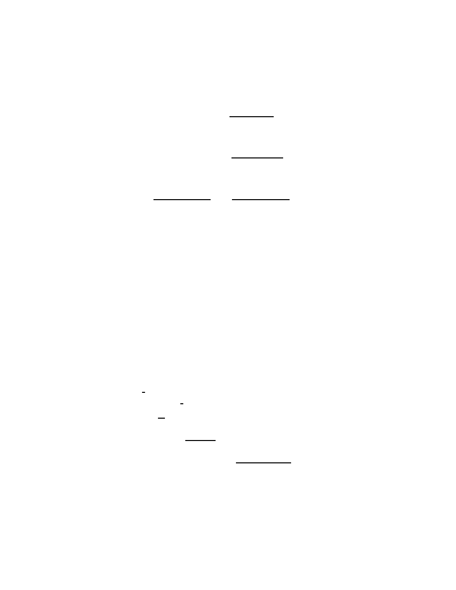
cosh(χ) d(χ) = 4
(4 + r
2
) d(r)
(
−4 + r
2
)
2
cosh(χ)
2
d(χ)
2
= 16
(4 + r
2
)
2
d(r)
2
(
−4 + r
2
)
4
(4 + r
2
)
2
d(χ)
2
(r
− 2)
2
(r + 2)
2
= 16
(4 + r
2
)
2
d(r)
2
(r
− 2)
4
(r + 2)
4
And finally
>
coord := [r, theta, phi]:# spherical coordinates
>
g_compts_hyp :=\
>
array(symmetric,sparse,1..3,1..3):# metric components
>
g_compts_hyp[1,1] :=\
>
-2/R:# component of interval\
>
attached to d(chi)^2
>
g_compts_hyp[2,2] :=\
>
(-2/R)*sinh(chi)^2:# component of interval\
>
attached to d(theta)^2
>
g_compts_hyp[3,3] :=\
>
(-2/R)*sinh(chi)^2*sin(theta)^2:# component\
>
of interval attached to d(phi)^2
>
g_hyp :=\
>
create([-1,-1], eval(g_compts_hyp));# covariant\
>
metric tensor
g hyp :=
table([index char = [
−1, −1], compts =
−2
1
R
0
0
0
−2
sinh(χ)
2
R
0
0
0
−2
sinh(χ)
2
sin(θ)
2
R
])
Here R/2 is the Gaussian curvature K (K <0). So, the linear element is
>
l_hyp := d(s)^2 = a^2*(d(chi)^2 +\
>
sinh(chi)^2*(d(theta)^2+sin(theta)^2*d(phi)^2));
77
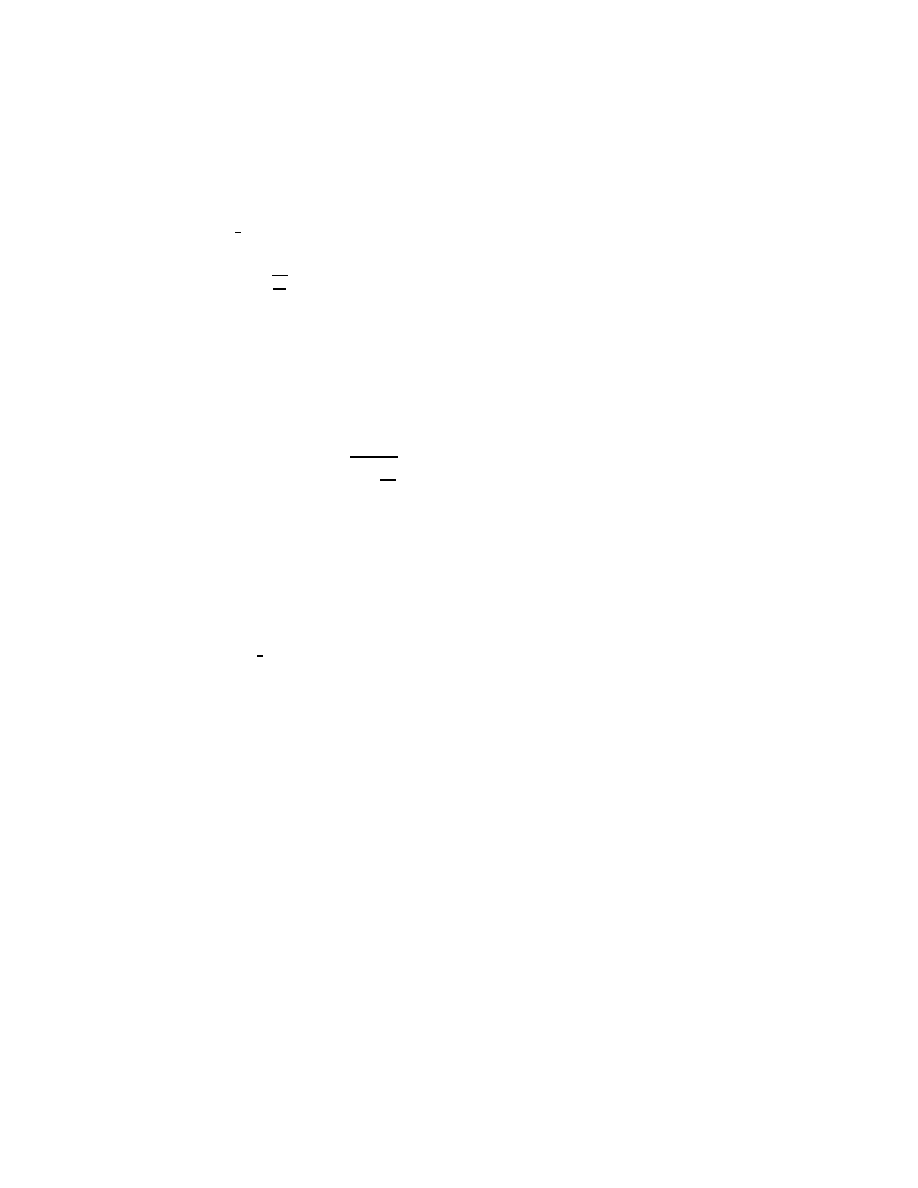
l hyp := d(s)
2
= a
2
(d(χ)
2
+ sinh(χ)
2
(d(θ)
2
+ sin(θ)
2
d(φ)
2
))
where a =
q
1
K
is the imaginary scale factor. The substitution r = a sinh(
χ ) results in:
>
subs(\
>
{sinh(chi)=r/a,d(chi)^2=d(r)^2/(a^2*(1+r^2/a^2))},\
>
l_hyp):#we use d(r)=a*cosh(chi)*d(chi)
>
expand(%);
d(s)
2
=
d(r)
2
1 +
r
2
a
2
+ r
2
d(θ)
2
+ r
2
sin(θ)
2
d(φ)
2
At last, for flat space:
>
l_flat := d(s)^2 = a^2*(d(chi)^2 +\
>
chi^2*(d(theta)^2+sin(theta)^2*d(phi)^2));
l flat := d(s)
2
= a
2
(d(χ)
2
+ χ
2
(d(θ)
2
+ sin(θ)
2
d(φ)
2
))
Here a is the arbitrary scaling factor.
To imagine the considered geometries we can use the usual technique of
embedding. In the general case the imbedding of 3-space is not possible
if the dimension of enveloping flat space is only 4 (we have 6 functions
g
i, j
, but the number of free parameters in 4-dimensional space is only 4).
However, the constant nonzero curvature allows to embed our curved space
in 4-dimensional flat space as result of next transformation of coordinates
(for spherical geometry):
>
defform(f=0,w1=1,w2=1,w3=1,v=1,chi=0,theta=0,phi=0);
>
e_1 := Dw^2 = a^2*d(cos(chi))^2;
>
e_2 := Dx^2 =\
>
(a*d(sin(chi)*sin(theta)*cos(phi)))^2;
>
e_3 := Dy^2 =\
>
(a*d(sin(chi)*sin(theta)*sin(phi)))^2;
>
e_4 := Dz^2 =\
>
(a*d(sin(chi)*cos(theta)))^2;
78

e 1 := Dw
2
= a
2
sin(χ)
2
d(χ)
2
e 2 := Dx
2
= a
2
(sin(θ) cos(φ) cos(χ) d(χ) + sin(χ) cos(φ) cos(θ) d(θ)
−
sin(χ) sin(θ) sin(φ) d(φ))
2
e 3 := Dy
2
= a
2
(sin(θ) sin(φ) cos(χ) d(χ) + sin(χ) sin(φ) cos(θ) d(θ)+
sin(χ) sin(θ) cos(φ) d(φ))
2
e 4 := Dz
2
= a
2
(cos(θ) cos(χ) d(χ)
− sin(χ) sin(θ) d(θ))
2
>
#so we have for Euclidian 4-metric:
>
simplify(\
>
rhs(e_1) + rhs(e_2) + rhs(e_3) + rhs(e_4), trig);
a
2
(d(φ)
2
cos(χ)
2
cos(θ)
2
+ d(θ)
2
+ d(φ)
2
− d(θ)
2
cos(χ)
2
−
d(φ)
2
cos(θ)
2
− d(φ)
2
cos(χ)
2
+ d(χ)
2
)
>
collect(%,d(phi)^2);
a
2
(1
− cos(θ)
2
− cos(χ)
2
+ cos(χ)
2
cos(θ)
2
) d(φ)
2
+
a
2
(d(θ)
2
+ d(χ)
2
− d(θ)
2
cos(χ)
2
)
This expression can be easily converted in l sp, i. e. the imbedding is correct.
Since
>
w^2 + x^2 + y^2 + z^2 =\
>
simplify(\
>
(a*cos(chi))^2 +(a*sin(chi)*sin(theta)*cos(phi))^2 +\
>
(a*sin(chi)*sin(theta)*sin(phi))^2 +\
>
(a*sin(chi)*cos(theta))^2);
w
2
+ x
2
+ y
2
+ z
2
= a
2
the considered hypersurface is the 3-sphere in flat 4-space. The scale factor
is the radius of the closed spherical universe.
In the case l hyp there is not the imbedding in flat Euclidian 4-space, but
there is the imbedding in flat hyperbolical flat space with interval
79

-d w
2
+ d x
2
+ d y
2
+ d z
2
As result we have
>
w^2 - x^2 - y^2 - z^2 =\
>
simplify(\
>
(a*cosh(chi))^2 - (a*sinh(chi)*sin(theta)*cos(phi))^2 -\
>
(a*sinh(chi)*sin(theta)*sin(phi))^2 -\
>
(a*sinh(chi)*cos(theta))^2);
w
2
− x
2
− y
2
− z
2
= a
2
This is expression for 3-hyperboloid in flat 4-space.
4.3
Standard models
Now we turn to some specific isotropic and homogeneous models. The as-
sumption of time-dependent character of the geometry results in the time-
dependence of scaling factor a(t). Then 4-metric (spherical geometry) is
>
coord := [t, chi, theta, phi]:
>
g_compts := array(symmetric,sparse,1..4,1..4):
>
g_compts[1,1] := -1:#dt^2
>
g_compts[2,2] := a(t)^2:#chi^2
>
g_compts[3,3]:=a(t)^2*sin(chi)^2:#dtheta^2
>
g_compts[4,4]:=a(t)^2*sin(chi)^2*sin(theta)^2:#dphi^2
>
g := create([-1,-1], eval(g_compts));
>
ginv := invert( g, ’detg’ ):
g := table([index char = [
−1, −1], compts =
−1
0
0
0
0 a(t)
2
0
0
0
0
a(t)
2
sin(χ)
2
0
0
0
0
a(t)
2
sin(χ)
2
sin(θ)
2
])
The Einstein tensor is
>
D1g := d1metric( g, coord ):
>
D2g := d2metric( D1g, coord ):
>
Cf1 := Christoffel1 ( D1g ):
>
RMN := Riemann( ginv, D2g, Cf1 ):
>
RICCI := Ricci( ginv, RMN ):
>
RS := Ricciscalar( ginv, RICCI ):
>
G := Einstein( g, RICCI, RS );
80

G := table([index char = [
−1, −1],
compts =
−2 sin(χ)
2
− 3 (
∂
∂t
a(t))
2
sin(χ)
2
− 1 + cos(χ)
2
a(t)
2
sin(χ)
2
, 0 , 0 , 0
0 ,
−
−2 a(t) sin(χ)
2
(
∂
2
∂t
2
a(t))
− (
∂
∂t
a(t))
2
sin(χ)
2
− 1 + cos(χ)
2
sin(χ)
2
, 0 , 0
0 , 0 , 2 a(t) sin(χ)
2
(
∂
2
∂t
2
a(t)) + sin(χ)
2
+ (
∂
∂t
a(t))
2
sin(χ)
2
, 0
0 , 0 , 0 , 2 a(t) sin(χ)
2
sin(θ)
2
(
∂
2
∂t
2
a(t)) + sin(θ)
2
sin(χ)
2
+ (
∂
∂t
a(t))
2
sin(χ)
2
sin(θ)
2
])
Let’s the matter is defined by the energy-momentum tensor T
µ, ν
= (p+ ρ )
u
µ
u
ν
+p g
µ, ν
:
>
T_compts :=\
>
array(symmetric,sparse,1..4,1..4):# energy-momentum\
>
tensor for drop of liquid
>
T_compts[1,1] := rho(t):
>
T_compts[2,2] := a(t)^2*p(t):
>
T_compts[3,3] := a(t)^2*sin(chi)^2*p(t):
>
T_compts[4,4] :=\
>
a(t)^2*sin(chi)^2*sin(theta)^2*p(t):
>
T := create([-1,-1], eval(T_compts));
T := table([index char = [
−1, −1], compts =
ρ(t)
0
0
0
0
a(t)
2
p(t)
0
0
0
0
a(t)
2
sin(χ)
2
p(t)
0
0
0
0
a(t)
2
sin(χ)
2
sin(θ)
2
p(t)
])
Then the first Einstein equation G
0, 0
- Λ g
0, 0
= - 8 π T
0, 0
(we add the
so-called cosmological constant Λ , which can be considered as the energy
density of vacuum):
81

>
get_compts(G):
>
%[1,1]:
>
e1 := simplify(%):
>
get_compts(g):
>
%[1,1]:
>
e2 := simplify(%):
>
get_compts(T):
>
%[1,1]:
>
e3 := simplify(%):
>
E[1] := expand(e1/(-3)) = -8*Pi*expand(e3/(-3)) +\
>
expand(e2*Lambda/(-3));#first Einstein equation
E
1
:=
1
a(t)
2
+
(
∂
∂t
a(t))
2
a(t)
2
=
8
3
π ρ(t) +
1
3
Λ
Second equation is:
>
get_compts(G):
>
%[2,2]:
>
e1 := simplify(%):
>
get_compts(g):
>
%[2,2]:
>
e2 := simplify(%):
>
get_compts(T):
>
%[2,2]:
>
e3 := simplify(%):
>
E[2] :=\
>
expand(e1/a(t)^2) = -8*Pi*expand(e3/a(t)^2) +\
>
expand(e2*Lambda/a(t)^2);#second Einstein equation
E
2
:= 2
∂
2
∂t
2
a(t)
a(t)
+
(
∂
∂t
a(t))
2
a(t)
2
+
1
a(t)
2
=
−8 π p(t) + Λ
Two other equations are tautological.
After elementary transformation we have for the second equation:
>
expand(simplify(E[2]-E[1])/2);
∂
2
∂t
2
a(t)
a(t)
=
−4 π p(t) +
1
3
Λ
−
4
3
π ρ(t)
Similarly, for the hyperbolical geometry we have:
82
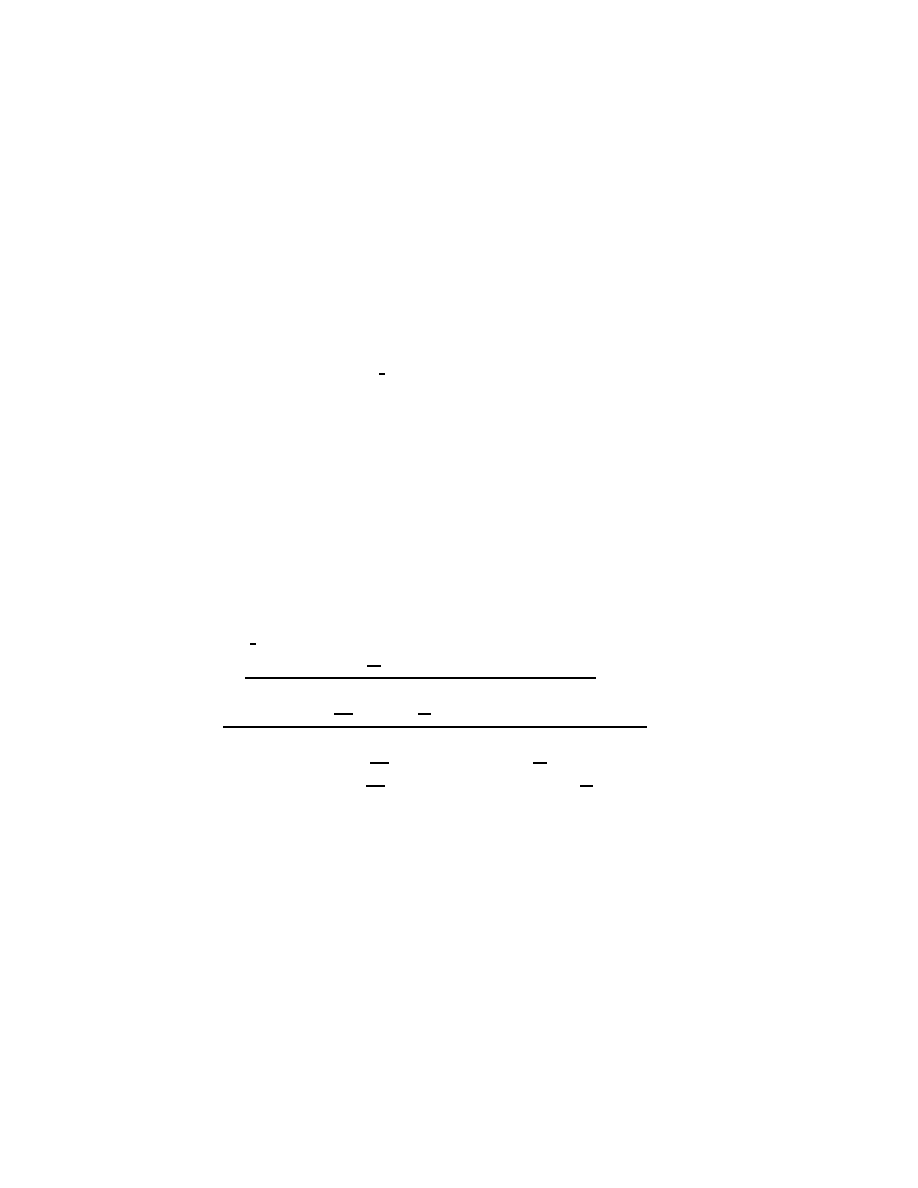
>
coord := [t, chi, theta, phi]:
>
g_compts := array(symmetric,sparse,1..4,1..4):
>
g_compts[1,1] := -1:#dt^2
>
g_compts[2,2] := a(t)^2:#chi^2
>
g_compts[3,3]:=a(t)^2*sinh(chi)^2:#dtheta^2
>
g_compts[4,4]:=\
>
a(t)^2*sinh(chi)^2*sin(theta)^2:#dphi^2
>
g := create([-1,-1], eval(g_compts));
>
ginv := invert( g, ’detg’ ):
g := table([index char = [
−1, −1], compts =
−1
0
0
0
0 a(t)
2
0
0
0
0
a(t)
2
sinh(χ)
2
0
0
0
0
a(t)
2
sinh(χ)
2
sin(θ)
2
])
>
D1g := d1metric( g, coord ):
>
D2g := d2metric( D1g, coord ):
>
Cf1 := Christoffel1 ( D1g ):
>
RMN := Riemann( ginv, D2g, Cf1 ):
>
RICCI := Ricci( ginv, RMN ):
>
RS := Ricciscalar( ginv, RICCI ):
>
G := Einstein( g, RICCI, RS );
G := table([index char = [
−1, −1], compts =
−
−2 sinh(χ)
2
+ 3 (
∂
∂t
a(t))
2
sinh(χ)
2
+ 1
− cosh(χ)
2
a(t)
2
sinh(χ)
2
, 0 , 0 , 0
0 ,
2 a(t) sinh(χ)
2
(
∂
2
∂t
2
a(t)) + (
∂
∂t
a(t))
2
sinh(χ)
2
+ 1
− cosh(χ)
2
sinh(χ)
2
, 0 , 0
0 , 0 , 2 a(t) sinh(χ)
2
(
∂
2
∂t
2
a(t))
− sinh(χ)
2
+ (
∂
∂t
a(t))
2
sinh(χ)
2
, 0
0 , 0 , 0 , 2 a(t) sinh(χ)
2
sin(θ)
2
(
∂
2
∂t
2
a(t))
− sin(θ)
2
sinh(χ)
2
+ (
∂
∂t
a(t))
2
sinh(χ)
2
sin(θ)
2
])
>
T_compts :=\
>
array(symmetric,sparse,1..4,1..4):# energy-momentum\
>
tensor for drop of liquid
>
T_compts[1,1] := rho(t):
>
T_compts[2,2] := a(t)^2*p(t):
>
T_compts[3,3] := a(t)^2*sinh(chi)^2*p(t):
>
T_compts[4,4] := a(t)^2*sinh(chi)^2*sin(theta)^2*p(t):
>
T := create([-1,-1], eval(T_compts));
83
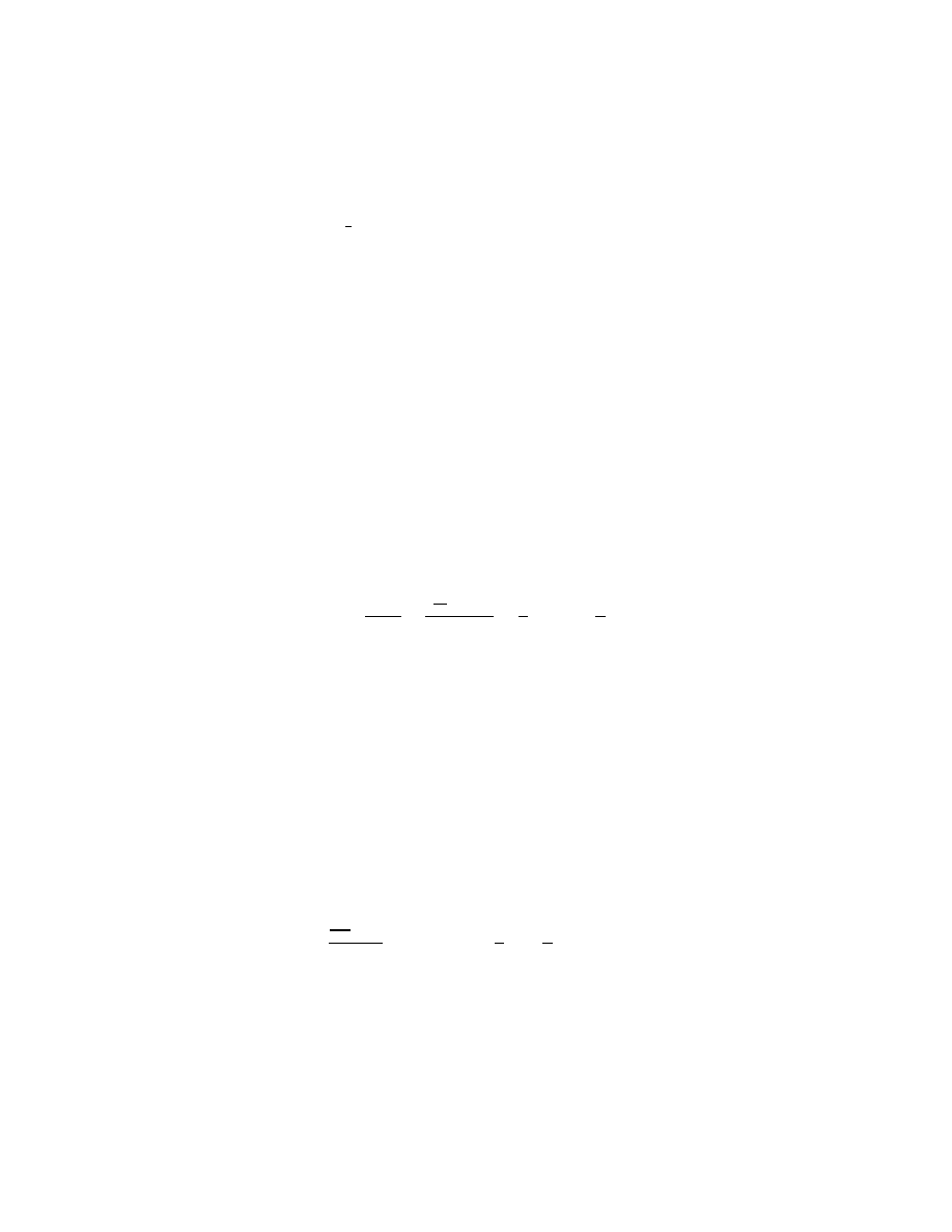
T := table([index char = [
−1, −1], compts =
ρ(t)
0
0
0
0
a(t)
2
p(t)
0
0
0
0
a(t)
2
sinh(χ)
2
p(t)
0
0
0
0
a(t)
2
sinh(χ)
2
sin(θ)
2
p(t)
])
>
get_compts(G):
>
%[1,1]:
>
e1 := simplify(%):
>
get_compts(g):
>
%[1,1]:
>
e2 := simplify(%):
>
get_compts(T):
>
%[1,1]:
>
e3 := simplify(%):
>
E[1] :=\
>
expand(e1/(-3)) = -8*Pi*expand(e3/(-3)) +\
>
expand(e2*Lambda/(-3));#first Einstein equation
E
1
:=
−
1
a(t)
2
+
(
∂
∂t
a(t))
2
a(t)
2
=
8
3
π ρ(t) +
1
3
Λ
>
get_compts(G):
>
%[2,2]:
>
e1 := simplify(%):
>
get_compts(g):
>
%[2,2]:
>
e2 := simplify(%):
>
get_compts(T):
>
%[2,2]:
>
e3 := simplify(%):
>
E[2] :=\
>
expand(e1/a(t)^2) = -8*Pi*expand(e3/a(t)^2) +\
>
expand(e2*Lambda/a(t)^2):#second Einstein equation
>
expand(simplify(E[2]-E[1])/2);
∂
2
∂t
2
a(t)
a(t)
=
−4 π p(t) +
1
3
Λ
−
4
3
π ρ(t)
The second equation is identical with one in spherical geometry.
In general, the first and second differential equations for scaling factor in
our ideal universe:
84
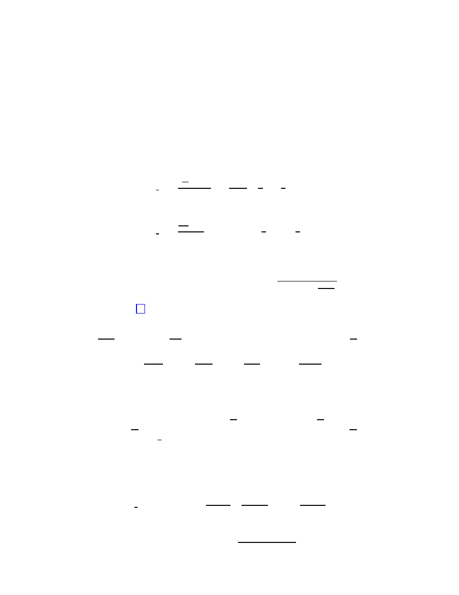
>
basic_1 :=\
>
(diff(a(t),t)/a(t))^2 = -K/a(t)^2 + Lambda/3 +\
>
8*Pi*rho(t)/3;#first basic equation for\
>
homogeneous universe
>
basic_2 :=\
>
diff(a(t),‘$‘(t,2))/a(t) =\
>
-4*Pi*(p(t)+rho(t)/3)+1/3*Lambda;# second\
>
basic equation for homogeneous universe
basic 1 :=
(
∂
∂t
a(t))
2
a(t)
2
=
−
K
a(t)
2
+
1
3
Λ +
8
3
π ρ(t)
basic 2 :=
∂
2
∂t
2
a(t)
a(t)
=
−4 π (p(t) +
1
3
ρ(t)) +
1
3
Λ
Here K =+1 for spherical, -1 for hyperbolical and 0 for flat geometries. The
left-hand side of the first equation is the square of Hubble constant H. If
we denote recent value of this parameter as H
0
, then H
0
= 65
km
s Mpc
(ps is
the parallax second corresponding to distance about of 3.26 light-years or
3* 10
13
km) [11].
When K= Λ =0, the universe is defined by the so-called critical density ρ
c
=
3 H
0
2
8 π
=7.9* 10
(
−30)
g
cm
3
. Let’s denote the recent relative values Ω
i
=
ρ
i
ρ
c
of the matter, radiation, cosmological constant and curvature as:
Ω
M
=
8 π ρ
M
3 H
0
2
, Ω
R
=
8 π ρ
R
3 H
0
2
, Ω
Λ
=
Λ
3 H
0
2
, Ω
K
= -
K
a
0
2
H
0
2
.
Here a
0
is the recent scaling factor. At this moment the contribution of the
radiation to density is negligible Ω
R
<< Ω
M
. To rewrite the evolutionary
equation in terms of Ω
i
we have to take into account the time dependence
of these parameters: Λ does not depend on a(t) (in framework of standard
model), the dependence of curvature ˜
1
a
2
, density of matter ˜
1
a
3
, but for
radiation ˜
1
a
4
. The last results from the change of density of quanta ˜
1
a
3
and their energy ˜
1
a
. The resulting equation can be written as:
>
basic_3 := H(a)^2 =\
>
H[0]^2*(Omega[R]*a[0]^4/a^4 + Omega[M]*a[0]^3/a^3\
>
+ Omega[Lambda] + Omega[K]*a[0]^2/a^2);
basic 3 := H(a)
2
= H
0
2
(
Ω
R
a
0
4
a
4
+
Ω
M
a
0
3
a
3
+ Ω
Λ
+
Ω
K
a
0
2
a
2
)
As result of these definitions we have the cosmic sum rule:
85

1 = Ω
M
+ Ω
R
+ Ω
Λ
+ Ω
K
.
Let us transit to the new variables: y=
a
a
0
, τ = H
0
( t
− t
0
), where t
0
is
the present time moment. Then
>
basic_4 :=\
>
diff(y(tau),tau) = sqrt(1 + (1/y(tau)-1)*Omega[M] +\
>
(y(tau)^2-1)*Omega[Lambda]);#we neglect the radiation\
>
contribution and use the cosmic sum rule.\
>
d(tau)=H[0]*d(t) --> a[0]*H[0]*(d(y)/d(tau))/a =\
>
(d(a)/d(t))/a = H
basic 4 :=
∂
∂τ
y(τ ) =
s
1 + (
1
y(τ )
− 1) Ω
M
+ (y(τ )
2
− 1) Ω
Λ
Now we will consider some typical standard models. For review see, for
example, [12], or on-line survey [13].
4.3.1
Einstein static
>
rhs(basic_1) = 0:
>
rhs(basic_2) = 0:
>
allvalues(\
>
solve(
{%, %%},{a(t), Lambda}) );# static universe
{Λ = 12 π p(t) + 4 π ρ(t), a(t) =
s
K
4 π p(t) + 4 π ρ(t)
},
{Λ = 12 π p(t) + 4 π ρ(t), a(t) = −
s
K
4 π p(t) + 4 π ρ(t)
}
At this moment for the matter p=0 and the contribution of the radiation is
small, therefore:
a
2
=
1
4 π ρ
, Λ = 4 π ρ
This solution has a very simple form and requires K = +1 (the closed
spherical universe) and positive Λ (repulsive action of vacuum), but does not
satisfy the observations of red shift in the spectra of extragalactic sources.
The last is the well-known fact demonstrating the expansion of universe (the
increase of scaling factor).
86
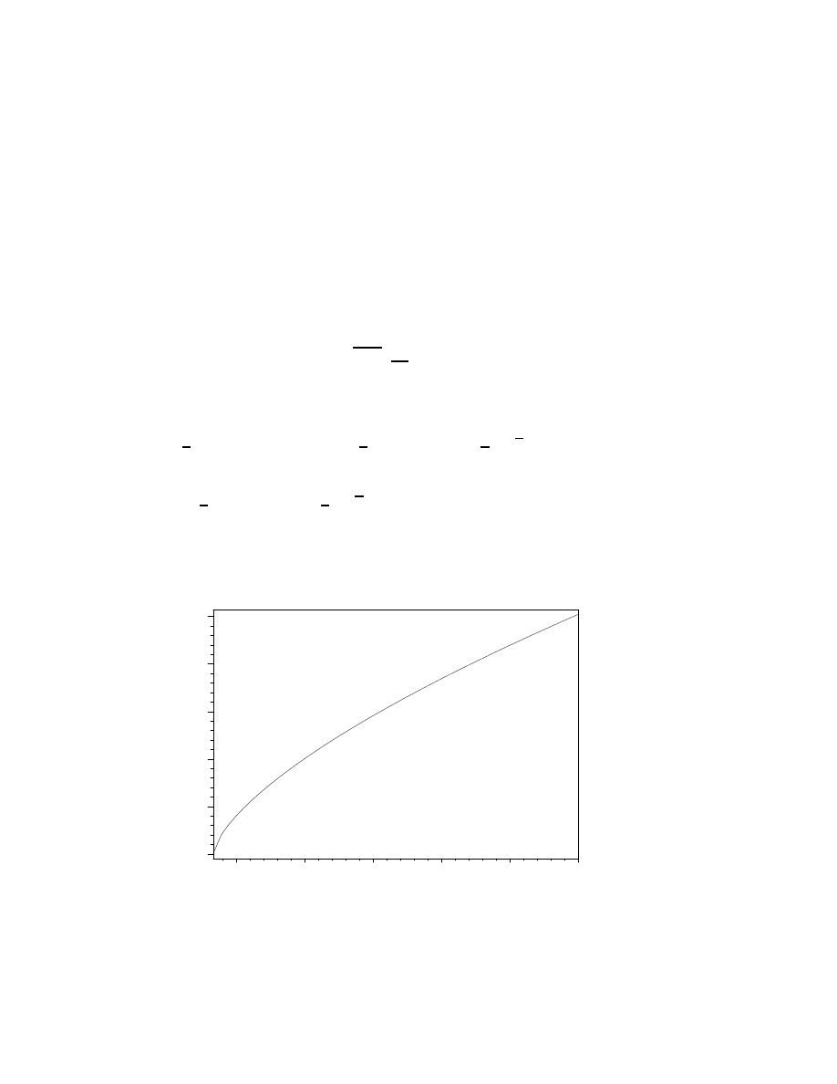
4.3.2
Einstein-de Sitter
Ω
M
= 1 and, as consequence Ω
Λ
= Ω
K
= 0. This is the flat universe
described by equation
>
y(tau)^(1/2)*diff(y(tau),tau) = 1;
>
dsolve(
{%, y(0)=1}, y(tau)):
>
allvalues(%);
q
y(τ ) (
∂
∂τ
y(τ )) = 1
y(τ ) =
1
4
(12 τ + 8)
(2/3)
, y(τ ) = (
−
1
4
(12 τ + 8)
(1/3)
+
1
4
I
√
3 (12 τ + 8)
(1/3)
)
2
,
y(τ ) =
(
−
1
4
(12 τ + 8)
(1/3)
−
1
4
I
√
3 (12 τ + 8)
(1/3)
)
2
>
plot(1/4*(12*tau+8)^(2/3), \
>
tau= -2/3..2, axes=BOXED,\
>
title=‘Einstein-de Sitter universe‘);
Einstein-de Sitter universe
0
0.5
1
1.5
2
2.5
–0.5
0
0.5
1
1.5
2
tau
We have the infinite expansion from the initial singularity (Big Bang).
87

From the value of scaling factor y(τ ) =
(12 τ +8)
( 2
3 )
4
it is possible to find the
universe’s age:
>
0 =\
>
(12*H[0]*(0-t[0]) + 8)^(2/3)/4:# y(0)=0
>
solve(%,t[0]);
2
3
1
H
0
>
evalf((2/3)*3*10^19/65/60/60/24/365);#[yr]
.9756859072 10
10
The obtained universe’s age does not satisfy the observations of the star’s
age in older globular clusters.
4.3.3
de Sitter and anti-de Sitter
The empty universes ( Ω
M
=0) with R > 0 (de Sitter) and R < 0 (anti-de
Sitter). Turning to basic 1 we have for de Sitter universe:
>
assume(lambda,positive):
>
subs(
{rho(t)=0,K=1,Lambda=lambda*3},\
>
basic_1):#lambda=Lambda/3
>
expand(%*a(t)^2);
>
dsolve(%,a(t));
(
∂
∂t
a(t))
2
=
−1 + a(t)
2
λ˜
a(t) =
1
√
λ˜
, a(t) =
−
1
√
λ˜
,
a(t) =
1
2
(1 +
%2
2
%1
2
) %1
%2
√
λ˜
, a(t) =
1
2
(1 +
%1
2
%2
2
) %2
%1
√
λ˜
%1 := e
( C1
√
λ˜)
%2 := e
(t
√
λ˜)
It is obvious, that the first two solutions don’t satisfy the basic 2. Another
88
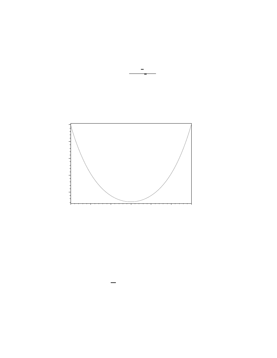
solutions give:
a(t) =
cosh(
√
λ (t
−C))
2
√
λ
where C is the positive or negative constant defining the time moment cor-
responding to the minimal scaling factor.
>
plot(subs(lambda=0.5,\
>
cosh(sqrt(lambda)*tau)/2/sqrt(lambda)),\
>
tau=-3..3,title=‘de Sitter universe‘,axes=boxed);
de Sitter universe
1
1.5
2
2.5
3
–3
–2
–1
0
1
2
3
tau
For anti-de Sitter model we have:
>
assume(lambda,negative):
>
subs(
{rho(t)=0,K=-1,Lambda=lambda*3},\
>
basic_1):#lambda=Lambda/3
>
expand(%*a(t)^2);
>
dsolve(%,a(t));
(
∂
∂t
a(t))
2
= 1 + a(t)
2
λ˜
89
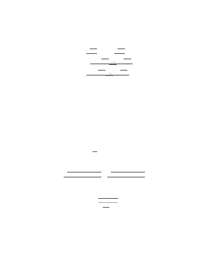
a(t) =
√
−λ˜
λ˜
, a(t) =
−
√
−λ˜
λ˜
,
a(t) =
−
sin(t
√
−λ˜ − C1
√
−λ˜)
√
−λ˜
,
a(t) =
sin(t
√
−λ˜ − C1
√
−λ˜)
√
−λ˜
De Sitter and anti-de Sitter universes play a crucial role in many modern
issues in GR and cosmology, in particular, in inflationary scenarios of the
beginning of universe evolution.
4.3.4
Closed Friedmann-Lemaitre
Ω
M
> 1 Λ = 0 and, as consequence Ω
K
< 0 (K =+1). This is the closed
spherical universe.
>
y(tau)*(diff(y(tau),tau)^2+b) =\
>
Omega[M];# b=Omega[M]-1 > 0
y(τ ) ((
∂
∂τ
y(τ ))
2
+ b) = Ω
M
>
solve( %,diff(y(tau),tau) );
p
y(τ ) (
−y(τ) b + Ω
M
)
y(τ )
,
−
p
y(τ ) (
−y(τ) b + Ω
M
)
y(τ )
>
d(t)=sqrt(y/b/(Omega[M]/b - y))*d(y);
d(t) =
v
u
u
t
y
b (
Ω
M
b
− y)
d(y)
Introducing a new variable φ we have :
>
sqrt(y/(Omega[M]/b - y)) = tan(phi);
>
y = solve(%, y);
>
y = convert(rhs(%),sincos);
90
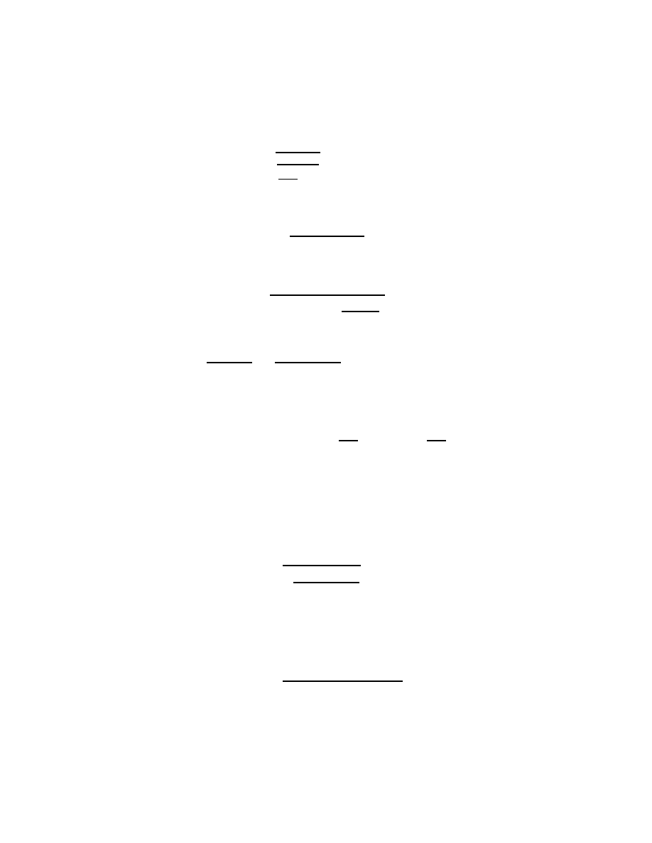
v
u
u
t
y
Ω
M
b
− y
= tan(φ)
y =
tan(φ)
2
Ω
M
b (1 + tan(φ)
2
)
y =
sin(φ)
2
Ω
M
cos(φ)
2
b (1 +
sin(φ)
2
cos(φ)
2
)
But this is y =
Ω
M
sin(φ)
2
b
=
Ω
M
(1
−cos(2 φ))
2 b
. And
>
defform(f=0,w1=0,w2=0,v=1,phi=0,y=0);
>
d(y) = d( (Omega[M]/b)*sin(phi)^2 );
d(y) = 2 sin(φ) cos(φ) (d(φ) &ˆ
Ω
M
b
) + sin(φ)
2
d(
Ω
M
b
)
Then our equation results in
>
subs(\
>
y=Omega[M]*sin(phi)^2/b,sqrt(y/(b*(Omega[M]/b-y))) ):
>
simplify(%);
s
−
−1 + cos(φ)
2
b cos(φ)
2
>
d(t) = simplify(\
>
(Omega[M]/b)*tan(phi)*2*sin(phi)*cos(phi))\
>
*d(phi)/sqrt(b);
d(t) =
−2
Ω
M
(
−1 + cos(φ)
2
) d(φ)
b
(3/2)
Hence, the age of universe is:
91
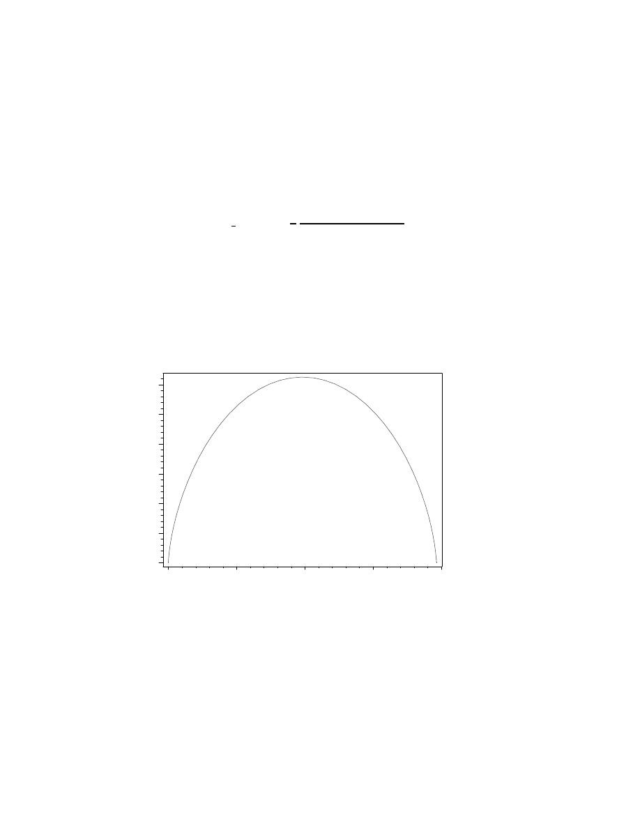
>
#initial conditions:
y(0)=0 --> phi=0
>
int( Omega[M]*(1-cos(2*x))/(Omega[M]-1)^(3/2),\
>
x=0..phi):
>
sol_1 := t = simplify(%);#age\
>
of universe vs phi
sol 1 := t =
−
1
2
Ω
M
(
−2 φ + sin(2 φ))
(Ω
M
− 1)
(3/2)
This equation in the combination with y( φ ) is the parametric representation
of cycloid:
>
y = Omega[M]*(1-cos(2*phi))/(2*(Omega[M]-1)):
>
plot([subs(Omega[M]=5,rhs(sol_1)),\
>
subs(Omega[M]=5,rhs(%)),phi=0..Pi], axes=boxed,\
>
title=‘closed Friedmann-Lemaitre universe‘);
closed Friedmann-Lemaitre universe
0
0.2
0.4
0.6
0.8
1
1.2
0
0.5
1
1.5
2
In this model the expansion from the singularity changes into contraction
and terminates in singularity (Big Crunch).
The age of universe is:
92
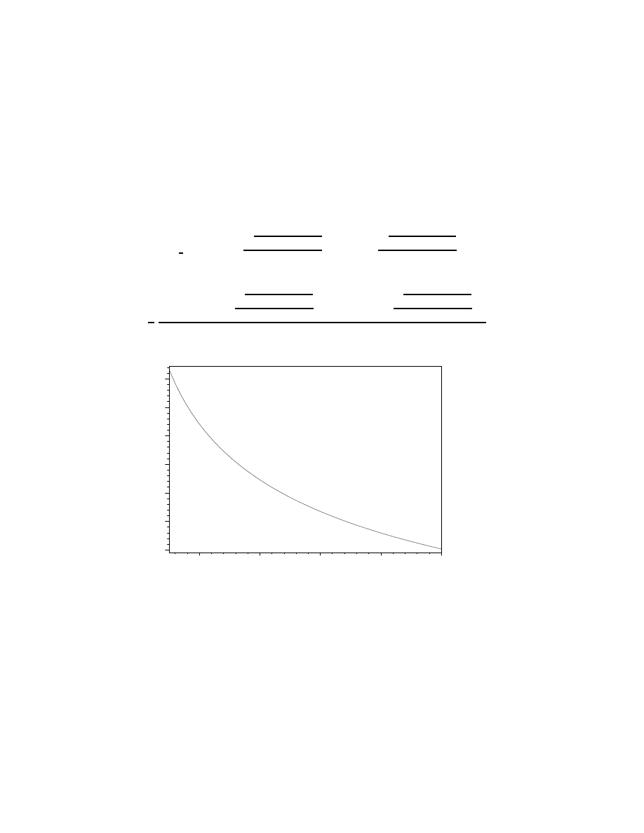
>
#initial conditions:
y(t0)=1 --> phi=?
>
1 = sin(phi)^2*Omega[M]/(Omega[M]-1):
>
sol_2 := solve(%,phi);
>
subs(phi=sol_2[1],rhs(sol_1));#age \
>
of universe vs Omega[M]
>
plot(%, Omega[M]=1.01..10, axes=BOXED, \
>
title=‘age of universe [1/H[0] ]‘);
sol 2 := arcsin(
p
Ω
M
(Ω
M
− 1)
Ω
M
),
−arcsin(
p
Ω
M
(Ω
M
− 1)
Ω
M
)
−
1
2
Ω
M
(
−2 arcsin(
p
Ω
M
(Ω
M
− 1)
Ω
M
) + sin(2 arcsin(
p
Ω
M
(Ω
M
− 1)
Ω
M
)))
(Ω
M
− 1)
(3/2)
age of universe [ 1/H[0] ]
0.35
0.4
0.45
0.5
0.55
0.6
0.65
2
4
6
8
10
Omega[M]
So, the increase of Ω
M
decreases the age of universe, which is less than
in Einstein-de Sitter model. The last and the modern observations of mi-
crowave background suggesting Ω
K
˜0 do not agree with this model.
4.3.5
Open Friedmann-Lemaitre
Ω
M
< 1 Λ = 0 and, as consequence Ω
K
> 0 (K = -1). This is the open
hyperbolical spherical universe. From the above introduced equation we
93

have
>
y(tau)*(diff(y(tau),tau)^2 - a) =\
>
Omega[M];# a = -b = 1-Omega[M]>0
y(τ ) ((
∂
∂τ
y(τ ))
2
− a) = Ω
M
>
solve( %,diff(y(tau),tau) );
p
y(τ ) (y(τ ) a + Ω
M
)
y(τ )
,
−
p
y(τ ) (y(τ ) a + Ω
M
)
y(τ )
>
diff(y(tau), tau)=sqrt((Omega[M] +\
>
a*y(tau))/y(tau));
∂
∂τ
y(τ ) =
s
y(τ ) a + Ω
M
y(τ )
>
dsolve(%, y(tau)):
>
sol_1 := simplify( subs(a=1-Omega[M],%),\
>
radical,symbolic);#implicit solution for y(tau)
sol 1 :=
−
1
2
(
−2 τ %1 Ω
M
+ Ω
M
ln(
−
1
2
−Ω
M
− 2 y(τ) + 2 y(τ) Ω
M
− 2
p
−y(τ) (−y(τ) + y(τ) Ω
M
− Ω
M
) %1
√
1
− Ω
M
)
− 2 C1 %1 Ω
M
+ 2 τ %1
− 2
p
−y(τ) (−y(τ) + y(τ) Ω
M
− Ω
M
) %1+
2 C1 %1)
.
(
√
1
− Ω
M
(Ω
M
− 1)) = 0
%1 :=
√
1
− Ω
M
>
#definition of _C1
>
subs(tau=1,sol_1):
>
subs(y(1)=1,%):
>
solve(%,_C1):
>
simplify( subs(_C1=%,sol_1) ):
>
subs(y(tau)=y,%):
>
sol_2 := solve(%,tau);#implicit solution\
>
with defined _C1
94
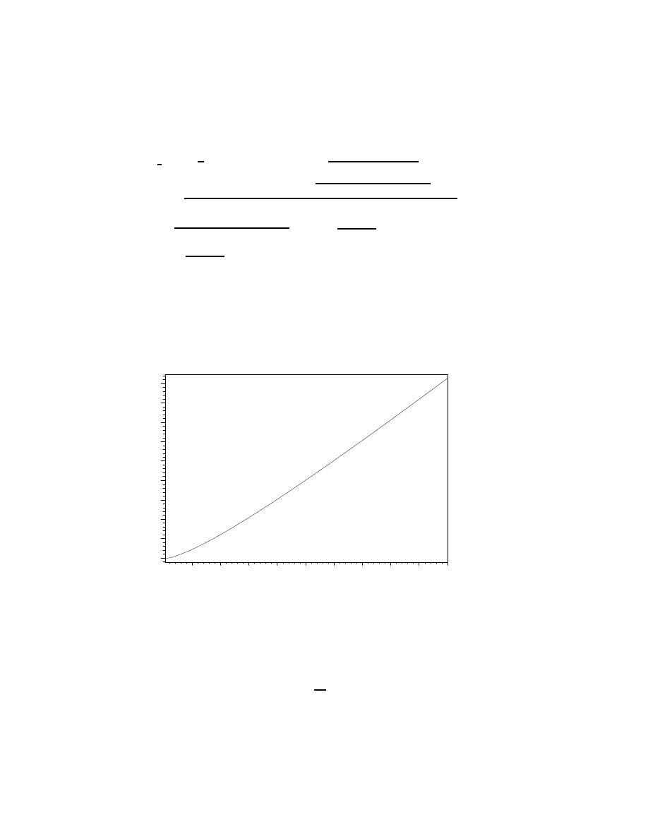
sol 2 :=
−
1
4
− 4 %1 Ω
M
+ Ω
M
ln(
−
(Ω
M
− 2 − 2 %1)
2
Ω
M
− 1
)
− ln
−
(Ω
M
+ 2 y
− 2 y Ω
M
+ 2
p
−y (−y + y Ω
M
− Ω
M
) %1)
2
Ω
M
− 1
!
Ω
M
+ 4
p
−y (−y + y Ω
M
− Ω
M
) %1
!
.
(
√
1
− Ω
M
(Ω
M
− 1))
%1 :=
√
1
− Ω
M
This solution can be plotted in the following form:
>
subs(Omega[M]=0.3,sol_2):
>
plot(%, y=0.01..2, axes=BOXED, colour=RED,\
>
title=‘hyperbolical universe\
>
(time vs scaling factor)‘ );
hyperbolical universe (time vs scaling factor)
0.2
0.4
0.6
0.8
1
1.2
1.4
1.6
1.8
2
0.2 0.4 0.6 0.8
1
1.2 1.4 1.6 1.8
2
y
The extreme case Ω
M
–>0 (almost empty world)
>
limit(sol_2,Omega[M]=0);
q
y
2
results in the linear low of universe expansion and gives the estimation for
maximal age of universe in this model:
95
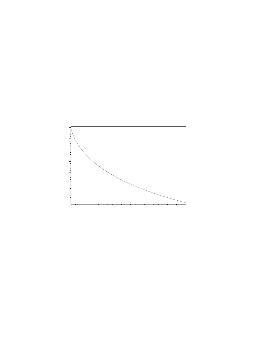
>
evalf(3*10^19/65/60/60/24/365);#[yr]
.1463528861 10
11
The dependence on Ω
M
looks as:
>
-(subs(y=0,sol_2)-subs(y=1,sol_2)):#age\
>
of universe [ 1/H[0] ]
>
plot(%, Omega[M]=0..1,axes=boxed,\
>
title=‘age of universe [ 1/H[0]]‘);
age of universe [ 1/H[0] ]
0.7
0.75
0.8
0.85
0.9
0.95
1
0
0.2
0.4
0.6
0.8
1
Omega[M]
It is natural, the growth of matter density decreases the universe age. If esti-
mations of Ω
M
give 0.3 (that results in the age
≈ 12 gigayears for considered
model), then this model does not satisfies the observations. Moreover, it is
possible, that the nonzero curvature is not appropriate (see below).
4.3.6
Expanding spherical and recollapsing hyperbolical universes
This model demonstrates the possibility of the infinite expansion of universe
with spherical geometry in the presence of nonzero cosmological constant.
96
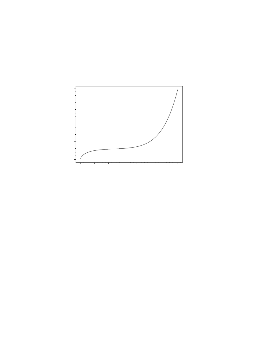
>
with(DEtools):
>
DEplot(subs(
{Omega[M]=1,Omega[Lambda]=2.59},\
>
basic_4),[y(tau)],tau=-2.5..1,[[y(0)=1]],stepsize=0.01,\
>
axes=boxed,linecolor=red,arrows=none,\
>
title=‘loitering expansion‘);
loitering expansion
0
1
2
3
4
y(tau)
–2.5
–2
–1.5
–1
–0.5
0
0.5
1
tau
We selected the parameters, which are close to ones for static universe (Ω
M
=1) but the cosmological term slightly dominates Ω
Λ
> 2 Ω
M
. There is the
delay of expansion, which looks like transition to collapse, but the domina-
tion of Ω
Λ
causes the further expansion. This model can explain the large
age of universe for large H
0
and to explain the misalignment in the ”red
shift-distance” distribution for distant quasars.
The next example demonstrate the collapsing behavior of an open (hyper-
bolical) universe:
>
p1 :=\
>
DEplot(subs(
{Omega[M]=0.5,Omega[Lambda]=-1},\
>
basic_4),[y(tau)],tau=-0.65..0.7,[[y(0)=1]],\
>
stepsize=0.01,axes=boxed,linecolor=red,\
>
arrows=none):#expansion
>
p2 :=\
>
DEplot(subs(
{Omega[M]=0.5,Omega[Lambda]=-1},\
>
lhs(basic_4)=-rhs(basic_4)),[y(tau)],\
>
tau=0.71..1.98,[[y(0.71)=1.36]],stepsize=0.01,\
>
axes=boxed,linecolor=red,arrows=none):#we have to\
>
change the sign in right-hand side of basic_4 and\
>
to change the initial condition
>
with(plots):
>
display(p1,p2,title=‘recollapsing open universe‘);
97
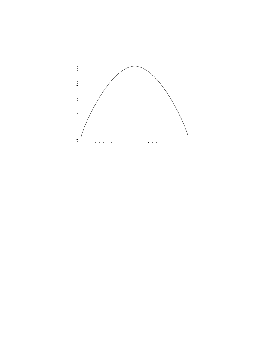
recollapsing open universe
0
0.2
0.4
0.6
0.8
1
1.2
1.4
y(tau)
–0.5
0
0.5
1
1.5
2
tau
4.3.7
Bouncing model
Main feature of the above considered nonstatic models (except for de Sitter
model) is the presence of singularity at the beginning of expansion and, it
is possible, at the end of evolution. On the one hand, the singularity is not
desirable, but, on the other hand, the standard model of Big Bang demands
a high-density and hot beginning of expansion. The last corresponds to the
conditions in the vicinity of the singularity. The choice of the parameters
allows the behavior without singularity:
>
p1 :=\
>
DEplot(subs(
{Omega[M]=0.1,Omega[Lambda]=1.5},basic_4),\
>
[y(tau)],tau=-1.13..1,[[y(0)=1]],stepsize=0.01,\
>
axes=boxed,linecolor=red,arrows=none):#expansion
>
p2 :=\
>
DEplot(subs(
{Omega[M]=0.1,Omega[Lambda]=1.5},\
>
lhs(basic_4)=-rhs(basic_4)),[y(tau)],tau=-3..-1.14,\
>
[[y(-3)=2.3]],stepsize=0.01,axes=boxed,linecolor=red,\
>
arrows=none):#contraction
>
display(p1,p2,title=‘bouncing universe‘);
98
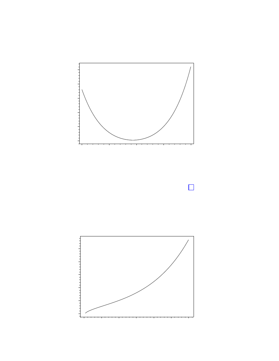
bouncing universe
0.5
1
1.5
2
2.5
3
y(tau)
–3
–2
–1
0
1
tau
4.3.8
Our universe (?)
The modern observations of microwave background suggest [11]: Ω
K
≈ 0
(flat), Ω
Λ
≈ 0.7, Ω
M
≈ 0.3. The corresponding behavior of scaling factor
looks as:
>
DEplot(subs(
{Omega[M]=0.3,Omega[Lambda]=0.7},\
>
basic_4),[y(tau)],tau=-.96...2,[[y(0)=1]],\
>
stepsize=0.01,axes=boxed,linecolor=red,arrows=none,\
>
title=‘ Our universe?
‘);
Our universe?
0
1
2
3
4
5
y(tau)
–1
–0.5
0
0.5
1
1.5
2
tau
99

We are to note, that our comments about appropriate (or not appropriate)
character of the considered models are not rigid. The picture of topologically
nontrivial space-time can combine the universes with the very different local
geometries and dynamics in the framework of a hypothetical Big Universe
(”Tree of Universes”).
4.4
Beginning
4.4.1
Bianchi models and Mixmaster universe
A good agreement of the isotropic homogeneous models with observations
does not provide for their validity nearby singularity. In particular, in frame-
work of analytical approach, we can refuse the isotropy of universe in the
beginning of expansion (for review see [14]). Let us consider the anisotropic
homogeneous flat universe without rotation:
>
coord := [t, x, y, z]:
>
g_compts :=\
>
array(symmetric,sparse,1..4,1..4):# metric components
>
g_compts[1,1] := -1:
>
g_compts[2,2] := a(t)^2:
>
g_compts[3,3] := b(t)^2:
>
g_compts[4,4] := c(t)^2:
>
g := create([-1,-1], eval(g_compts));
>
ginv := invert( g, ’detg’ ):
g := table([index char = [
−1, −1], compts =
−1
0
0
0
0 a(t)
2
0
0
0
0
b(t)
2
0
0
0
0
c(t)
2
])
The Einstein tensor is:
100
>
# intermediate values
>
D1g := d1metric( g, coord ):
>
D2g := d2metric( D1g, coord ):
>
Cf1 := Christoffel1 ( D1g ):
>
RMN := Riemann( ginv, D2g, Cf1 ):
>
RICCI := Ricci( ginv, RMN ):
>
RS := Ricciscalar( ginv, RICCI ):
>
Estn := Einstein( g, RICCI, RS ):# Einstein tensor
>
displayGR(Einstein,Estn);# Its nonzero components
The Einstein Tensor
non
− zero components :
G11 =
−
(
∂
∂t
b(t)) (
∂
∂t
a(t)) c(t) + (
∂
∂t
c(t)) (
∂
∂t
a(t)) b(t) + (
∂
∂t
c(t)) (
∂
∂t
b(t)) a(t)
a(t) b(t) c(t)
G22 =
a(t)
2
((
∂
2
∂t
2
b(t)) c(t) + (
∂
2
∂t
2
c(t)) b(t) + (
∂
∂t
c(t)) (
∂
∂t
b(t)))
b(t) c(t)
G33 =
b(t)
2
((
∂
2
∂t
2
a(t)) c(t) + (
∂
2
∂t
2
c(t)) a(t) + (
∂
∂t
c(t)) (
∂
∂t
a(t)))
a(t) c(t)
G44 =
c(t)
2
((
∂
2
∂t
2
a(t)) b(t) + (
∂
2
∂t
2
b(t)) a(t) + (
∂
∂t
b(t)) (
∂
∂t
a(t)))
a(t) b(t)
character : [
−1 , −1 ]
In the vacuum state the right-hand sides of Einstein equations are 0. Then
>
E_eqn := get_compts(Estn):
>
e1 := numer( E_eqn[1,1] ) = 0;
>
e2 :=\
>
expand( numer( E_eqn[2,2] )/a(t)^2 ) = 0;
>
e3 :=\
>
expand( numer( E_eqn[3,3] )/b(t)^2 ) = 0;
>
e4 :=\
>
expand( numer( E_eqn[4,4] )/c(t)^2 ) = 0;
101
e1 :=
−(
∂
∂t
b(t)) (
∂
∂t
a(t)) c(t)
− (
∂
∂t
c(t)) (
∂
∂t
a(t)) b(t)
−
(
∂
∂t
c(t)) (
∂
∂t
b(t)) a(t) = 0
e2 := (
∂
2
∂t
2
b(t)) c(t) + (
∂
2
∂t
2
c(t)) b(t) + (
∂
∂t
c(t)) (
∂
∂t
b(t)) = 0
e3 := (
∂
2
∂t
2
a(t)) c(t) + (
∂
2
∂t
2
c(t)) a(t) + (
∂
∂t
c(t)) (
∂
∂t
a(t)) = 0
e4 := (
∂
2
∂t
2
a(t)) b(t) + (
∂
2
∂t
2
b(t)) a(t) + (
∂
∂t
b(t)) (
∂
∂t
a(t)) = 0
We will search the power-behaved solutions of this system (Kasner metric):
>
e5 := simplify(\
>
subs(
{a(t)=a_0*t^p_1,b(t)=b_0*t^p_2,c(t)=c_0*t^p_3},\
>
e1) );
>
e6 := simplify(\
>
subs(
{a(t)=a_0*t^p_1,b(t)=b_0*t^p_2,c(t)=c_0*t^p_3},\
>
e2) );
>
e7 := simplify(\
>
subs(
{a(t)=a_0*t^p_1,b(t)=b_0*t^p_2,c(t)=c_0*t^p_3},\
>
e3) );
>
e8 := simplify(\
>
subs(
{a(t)=a_0*t^p_1,b(t)=b_0*t^p_2,c(t)=c_0*t^p_3},\
>
e4) );
e5 :=
−b 0 t
(p 2
−2+p 1 +p 3 )
p 2 a 0 p 1 c 0
− c 0 t
(p 2
−2+p 1 +p 3 )
p 3 a 0 p 1 b 0
− c 0 t
(p 2
−2+p 1 +p 3 )
p 3 b 0 p 2 a 0 = 0
e6 := b 0 t
(p 3
−2+p 2 )
p 2
2
c 0
− b 0 t
(p 3
−2+p 2 )
p 2 c 0
+ c 0 t
(p 3
−2+p 2 )
p 3
2
b 0
− c 0 t
(p 3
−2+p 2 )
p 3 b 0
+ c 0 t
(p 3
−2+p 2 )
p 3 b 0 p 2 = 0
e7 := a 0 t
(p 3
−2+p 1 )
p 1
2
c 0
− a 0 t
(p 3
−2+p 1 )
p 1 c 0
+ c 0 t
(p 3
−2+p 1 )
p 3
2
a 0
− c 0 t
(p 3
−2+p 1 )
p 3 a 0
+ c 0 t
(p 3
−2+p 1 )
p 3 a 0 p 1 = 0
102
e8 := a 0 t
(p 1
−2+p 2 )
p 1
2
b 0
− a 0 t
(p 1
−2+p 2 )
p 1 b 0
+ b 0 t
(p 1
−2+p 2 )
p 2
2
a 0
− b 0 t
(p 1
−2+p 2 )
p 2 a 0
+ b 0 t
(p 1
−2+p 2 )
p 2 a 0 p 1 = 0
If t is not equal to zero, we have:
>
e9 := factor( e5/t^(p_2-2+p_1+p_3) );
>
e10 := factor( e6/t^(p_3-2+p_2) );
>
e11 := factor( e7/t^(p_3-2+p_1) );
>
e12 := factor( e8/t^(p_2-2+p_1) );
e9 :=
−b 0 a 0 c 0 (p 2 p 1 + p 3 p 1 + p 3 p 2 ) = 0
e10 := b 0 c 0 (p 2
2
− p 2 + p 3
2
− p 3 + p 3 p 2 ) = 0
e11 := a 0 c 0 (p 1
2
− p 1 + p 3
2
− p 3 + p 3 p 1 ) = 0
e12 := a 0 b 0 (p 1
2
− p 1 + p 2
2
− p 2 + p 2 p 1 ) = 0
>
e13 := e9/(-b_0*a_0*c_0);
>
e14 := e10/(b_0*c_0);
>
e15 := e11/(a_0*c_0);
>
e16 := e12/(a_0*b_0);
e13 := p 2 p 1 + p 3 p 1 + p 3 p 2 = 0
e14 := p 2
2
− p 2 + p 3
2
− p 3 + p 3 p 2 = 0
e15 := p 1
2
− p 1 + p 3
2
− p 3 + p 3 p 1 = 0
e16 := p 1
2
− p 1 + p 2
2
− p 2 + p 2 p 1 = 0
The following manipulation gives a connection between parameters:
103
>
((e14 + e15 + e16) - e13)/2;
p 2
2
− p 2 + p 3
2
− p 3 + p 1
2
− p 1 = 0
That is p 1
2
+ p 2
2
+ p 3
2
= p 1 + p 2 + p 3 (3).
>
collect(e15-e16,
{p_2,p_3});
>
collect(e14-e15,
{p_1,p_2});
p 3
2
+ (p 1
− 1) p 3 − p 2
2
+ (1
− p 1 ) p 2 = 0
p 2
2
+ (p 3
− 1) p 2 − p 1
2
+ (1
− p 3 ) p 1 = 0
Hence
p 3 (p 3 + p 1 - 1) = p 2 (p 2 + p 1 - 1),
p 2 (p 3 + p 2 - 1) = p 1 (p 3 + p 1 - 1).
The last expressions suggest the simple solution:
(p 3 + p 1 - 1) = p 2, (p 2 + p 1 - 1) = p 3 and
(p 3 + p 2 - 1) = p 1, (p 3 + p 1 - 1) = p 2,
or
(p 3 + p 1 - 1) = - p 2, (p 2 + p 1 - 1) = - p 3 and
(p 3 + p 2 - 1) = - p 1, (p 3 + p 1 - 1) = - p 2
The first results in
>
p_3 + p_1 - 1 + p_2 + p_1 - 1 + p_3 + p_2\
>
- 1 - (p_1+p_2+p_3);
p 3 + p 1
− 3 + p 2
The second produces
104
>
(p_3 + p_1 - 1 + p_2 + p_1 - 1 +\
>
p_3 + p_2 - 1 + (p_1+p_2+p_3))/3;
p 3 + p 1
− 1 + p 2
These expressions in the combination with Eq.(3) suggest that there is only
one independent parameter p:
>
solve(
{p_1 + p_2 + p =\
>
1, p_1^2 + p_2^2 + p^2 = 1
},{p_1,p_2}):
>
sol_1 := allvalues(%);#first choice
>
solve(
{p_1 + p_2 + p = 3, p_1^2 + p_2^2 + p^2 = 3},\
>
{p_1,p_2}):
>
sol_2 := allvalues(%);#second choice
sol 1 :=
{p 1 = −
1
2
p +
1
2
−
1
2
%1, p 2 =
−
1
2
p +
1
2
+
1
2
%1
},
{p 1 = −
1
2
p +
1
2
+
1
2
%1, p 2 =
−
1
2
p +
1
2
−
1
2
%1
}
%1 :=
p
−3 p
2
+ 2 p + 1
sol 2 :=
{p 2 = −
1
2
p +
3
2
+
1
2
I (p
− 1)
√
3, p 1 =
−
1
2
p +
3
2
−
1
2
I (p
− 1)
√
3
},
{p 2 = −
1
2
p +
3
2
−
1
2
I (p
− 1)
√
3, p 1 =
−
1
2
p +
3
2
+
1
2
I (p
− 1)
√
3
}
So, if the parameters p 1, p 2, p 3 are real, we have p 1
2
+ p 2
2
+ p 3
2
=
p 1 + p 2 + p 3 =1 and
>
sol_p_1 := factor(subs(sol_1,p_1));
>
sol_p_2 := factor(subs(sol_1,p_2));
>
sol_p_3 := 1 - %% - %;
sol p 1 :=
−
1
2
p +
1
2
−
1
2
q
−(3 p + 1) (p − 1)
sol p 2 :=
−
1
2
p +
1
2
+
1
2
q
−(3 p + 1) (p − 1)
sol p 3 := p
105
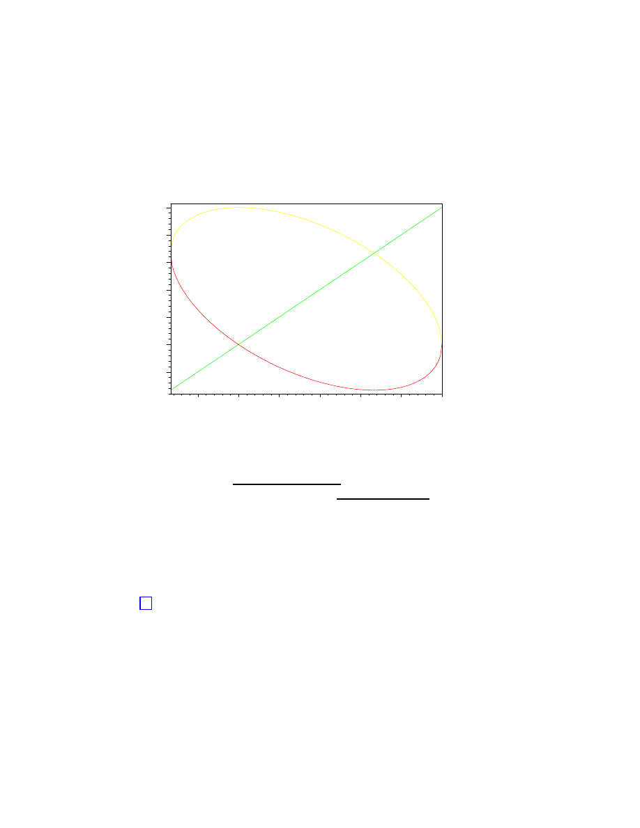
The values of the analyzed parameters are shown in the next figure:
>
plot(
{sol_p_1,sol_p_2,sol_p_3},p=-1/3..1,\
>
axes=boxed, title=‘powers of t‘);
powers of t
–0.2
0
0.2
0.4
0.6
0.8
1
–0.2
0
0.2
0.4
0.6
0.8
1
p
Hence, there are two directions of expansion and one direction of contraction
for t–>
∞ (so-called ”pancake” singularity) or one direction of expansion
and two direction of contraction for t–>0 (”sigar” singularity).
Now let’s consider more complicated situation with homogeneous anisotropic
metric.
We will use the tetrad notation of Einstein equations that allows to avoid
the explicit manipulations with coordinates. In the synchronous frame we
have for the homogeneous geometry (here Greek indexes change from 1 to
3) [15]:
g
0, 0
= -1, g
α, β
= η
a, b
(e
a
)
α
(e
b
)
β
,
where η
a, b
is the time dependent matrix, (e
a
)
α
is the frame vector (a changes
from 1 to 3, that is the number of space triad). We will use the following
representation for η :
106
>
eta :=\
>
array(\
>
[[a(t)^2,0,0],[0,b(t)^2,0],[0,0,c(t)^2]]);#a, b, c\
>
are the time-dependent coefficients of anisotropic\
>
deformation
>
eta_inv := inverse(eta):
>
kappa1 :=\
>
map(diff,eta,t):#kappa1[a,b]=diff(eta[a,b],t)
>
kappa2 := multiply(\
>
map(diff,eta,t),eta_inv);#kappa2[a]^b=\
>
diff(eta[a,b],t)*eta_inv, i.e.
we raise the index\
>
by eta_inv
η :=
a(t)
2
0
0
0
b(t)
2
0
0
0
c(t)
2
κ2 :=
2
∂
∂t
a(t)
a(t)
0
0
0
2
∂
∂t
b(t)
b(t)
0
0
0
2
∂
∂t
c(t)
c(t)
The first vacuum Einstein equation has a form
R
0
0
= -
1
2
∂
∂t
κ
a
a
-
1
4
κ
a
b
κ
b
a
= 0
>
eq_1 :=\
>
evalm( -trace(map(diff,kappa2,t))/2 -\
>
trace(multiply(kappa2,transpose(kappa2))/4) )\
>
= 0;#first Einstein equation
eq 1 :=
−
∂
2
∂t
2
a(t)
a(t)
−
∂
2
∂t
2
b(t)
b(t)
−
∂
2
∂t
2
c(t)
c(t)
= 0
The next Einstein equations demand the definition of Bianchi structured
constants: C
ab
= n
ab
+ e
abc
a
c
, (C
c
)
ab
= e
abd
C
dc
. Here e
abc
= e
abc
is
the unit antisymmetric symbol, n
ab
is the symmetric ”tensor”, which can
be expressed through its principal values n
i
, a
c
is the vector. The Bianchi
types are:
107

Type
a
n
1
n
2
n
3
I
0
0
0
0
II
0
1
0
0
VII
0
1
1
0
VI
0
1
-1
0
IX
0
1
1
1
VIII
0
1
1
-1
V
1
0
0
0
IV
1
0
0
1
VII
ζ
0
1
1
III (ζ=1), VI (ζ
6= 0) ζ
0
1
-1
Table 1: Bianchi constants
We will analyze type IX model, where C
11
= C
22
= C
33
= C
23
1
= C
31
2
=
C
12
3
= 1. The curvature P
a
b
=
1
2 η
{2 C
bd
C
ad
+ C
db
C
ad
+ C
bd
C
da
- C
d
d
( (C
b
)
a
+ C
a
b
) + δ
a
b
[ (C
d
)
d
2
-2 C
df
C
df
]
} is
>
Cab :=\
>
array([[1,0,0],[0,1,0],[0,0,1]]);#C^(ab)
>
C_ab := multiply(eta,eta,Cab);#C[ab]
>
Ca_b := multiply(eta,Cab);#C[a]^b
>
C_a_b := multiply(Cab,eta);#C^b[a];
>
delta := array([[1,0,0],[0,1,0],[0,0,1]]):
>
evalm( (4*multiply(Cab,C_ab) -\
>
trace(C_a_b)*evalm(C_a_b+Ca_b) +\
>
delta*(trace(C_a_b)^2 -\
>
2*trace(multiply(Cab,C_ab))))/(2*det(eta))):#here\
>
we use the diagonal form of eta and symmetry\
>
of structured constants
>
P := map(simplify,%);
Cab :=
1 0 0
0 1 0
0 0 1
C ab :=
a(t)
4
0
0
0
b(t)
4
0
0
0
c(t)
4
108

Ca b :=
a(t)
2
0
0
0
b(t)
2
0
0
0
c(t)
2
C a b :=
a(t)
2
0
0
0
b(t)
2
0
0
0
c(t)
2
P :=
−
1
2
−a(t)
4
+ b(t)
4
− 2 b(t)
2
c(t)
2
+ c(t)
4
a(t)
2
b(t)
2
c(t)
2
, 0 , 0
0 ,
−
1
2
−b(t)
4
+ a(t)
4
− 2 a(t)
2
c(t)
2
+ c(t)
4
a(t)
2
b(t)
2
c(t)
2
, 0
0 , 0 ,
1
2
c(t)
4
− a(t)
4
+ 2 a(t)
2
b(t)
2
− b(t)
4
a(t)
2
b(t)
2
c(t)
2
So, in the degenerate case a = b = c, t = const this model describes the
closed spherical universe with a positive scalar curvature.
Hence we can obtained the next group of vacuum Einstein equations:
R
a
b
= -
1
2 √η
[(
∂
∂t
√
η κ
a
b
) - P
a
b
] = 0
>
evalm(\
>
-map(diff,evalm(sqrt(det(eta))*kappa2),t)/\
>
(2*sqrt(det(eta)))):
>
evalm( map(simplify,%) - P );
109

−
(
∂
2
∂t
2
a(t)) b(t) c(t) + (
∂
∂t
b(t)) (
∂
∂t
a(t)) c(t) + (
∂
∂t
c(t)) (
∂
∂t
a(t)) b(t)
a(t) b(t) c(t)
+
1
2
(
−a(t)
4
+ b(t)
4
− 2 b(t)
2
c(t)
2
+ c(t)
4
)
a(t)
2
b(t)
2
c(t)
2
, 0 , 0
0 ,
−
(
∂
2
∂t
2
b(t)) a(t) c(t) + (
∂
∂t
b(t)) (
∂
∂t
a(t)) c(t) + (
∂
∂t
c(t)) (
∂
∂t
b(t)) a(t)
a(t) b(t) c(t)
+
1
2
(
−b(t)
4
+ a(t)
4
− 2 a(t)
2
c(t)
2
+ c(t)
4
)
a(t)
2
b(t)
2
c(t)
2
, 0
0 , 0 ,
−
(
∂
2
∂t
2
c(t)) a(t) b(t) + (
∂
∂t
c(t)) (
∂
∂t
a(t)) b(t) + (
∂
∂t
c(t)) (
∂
∂t
b(t)) a(t)
a(t) b(t) c(t)
−
1
2
c(t)
4
− a(t)
4
+ 2 a(t)
2
b(t)
2
− b(t)
4
a(t)
2
b(t)
2
c(t)
2
The obtained expression gives three Einstein equations:
>
eq_2 :=\
>
Diff( (diff(a(t),t)*b(t)*c(t)),t )/(a(t)*b(t)*c(t))\
>
= ((b(t)^2-c(t)^2)^2 - a(t)^4 )/\
>
(2*a(t)^2*b(t)^2*c(t)^2);
>
eq_3 :=\
>
Diff( (diff(b(t),t)*a(t)*c(t)),t )/(a(t)*b(t)*c(t))\
>
= ((a(t)^2-c(t)^2)^2 - b(t)^4 )/\
>
(2*a(t)^2*b(t)^2*c(t)^2);
>
eq_4 :=\
>
Diff( (diff(c(t),t)*b(t)*a(t)),t )/(a(t)*b(t)*c(t))\
>
= ((a(t)^2-b(t)^2)^2 - c(t)^4 )/\
>
(2*a(t)^2*b(t)^2*c(t)^2);
eq 2 :=
∂
∂t
(
∂
∂t
a(t)) b(t) c(t)
a(t) b(t) c(t)
=
1
2
(b(t)
2
− c(t)
2
)
2
− a(t)
4
a(t)
2
b(t)
2
c(t)
2
eq 3 :=
∂
∂t
(
∂
∂t
b(t)) a(t) c(t)
a(t) b(t) c(t)
=
1
2
(a(t)
2
− c(t)
2
)
2
− b(t)
4
a(t)
2
b(t)
2
c(t)
2
110
eq 4 :=
∂
∂t
(
∂
∂t
c(t)) b(t) a(t)
a(t) b(t) c(t)
=
1
2
(a(t)
2
− b(t)
2
)
2
− c(t)
4
a(t)
2
b(t)
2
c(t)
2
The last group of Einstein equations results from
R
a
0
= -
1
2
κ
b
c
( (C
b
)
ca
- δ
a
b
(C
d
)
dc
) = 0
It is obvious, that in our case this equation is identically zero (see expression
for (C
b
)
ca
). The substitutions of a= e
α
, b= e
β
, c= e
γ
(do not miss these
exponents with frame vectors!), dt=a b c (d τ ) and the expressions
∂
∂t
a =
∂
∂τ
a
∂
∂t
τ =
∂
∂τ
a
a b c
=
∂
∂τ
α
b c
and
∂
2
∂t
2
a =
1
a b c
∂
∂τ
∂
∂τ
α
b c
=
1
a b c
[
∂2
∂τ 2
α
b c
- (
(
∂
∂τ
γ)+(
∂
∂τ
β)
b c
)
∂
∂τ
α ] result in the simplification of the equations form:
>
eq_1 :=\
>
diff((alpha(tau)+beta(tau)+gamma(tau)), tau$2)/2 =\
>
diff(alpha(tau), tau)*diff(beta(tau),tau) +\
>
diff(alpha(tau),tau)*diff(gamma(tau),tau) +\
>
diff(beta(tau),tau)*diff(gamma(tau),tau);
>
eq_2 :=\
>
2*diff(alpha(tau),tau$2) = (b(t)^2-c(t)^2)^2-a(t)^4;
>
eq_3 :=\
>
2*diff(beta(tau),tau$2) = (a(t)^2-c(t)^2)^2-b(t)^4;
>
eq_4 :=\
>
2*diff(gamma(tau),tau$2) = (a(t)^2-b(t)^2)^2-c(t)^4;
eq 1 :=
1
2
(
∂
2
∂τ
2
α(τ )) +
1
2
(
∂
2
∂τ
2
β(τ )) +
1
2
(
∂
2
∂τ
2
γ(τ )) =
(
∂
∂τ
α(τ )) (
∂
∂τ
β(τ )) + (
∂
∂τ
α(τ )) (
∂
∂τ
γ(τ )) + (
∂
∂τ
β(τ )) (
∂
∂τ
γ(τ ))
eq 2 := 2 (
∂
2
∂τ
2
α(τ )) = (b(t)
2
− c(t)
2
)
2
− a(t)
4
eq 3 := 2 (
∂
2
∂τ
2
β(τ )) = (a(t)
2
− c(t)
2
)
2
− b(t)
4
eq 4 := 2 (
∂
2
∂τ
2
γ(τ )) = (a(t)
2
− b(t)
2
)
2
− c(t)
4
Comparison of obtained equations with above considered Kasner’s type
equations suggests that these systems are identical if the right-hand sides
111
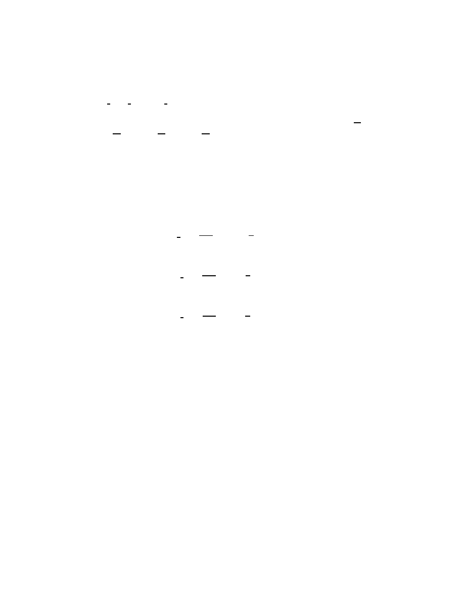
of eq 2, eq 3 and eq 4 are equal to zero. Therefore we will consider the
system’s evolution as dynamics of Kasner’s solution perturbation. In this
case τ = ln(t) + const (dt=a b c d τ = t
(p
1
+p
2
+p
3
)
d τ , as result d τ =
dt
t
) and
∂
∂τ
α = p
1
,
∂
∂τ
β = p
2
,
∂
∂τ
γ = p
3
. We assume that the right-hand
sides are close to zero, but contribution of e
(4 α)
- terms dominates. Hence:
>
eq_5 := diff(alpha(tau),‘$‘(tau,2)) =\
>
-exp(4*alpha(tau))/2;
>
eq_6 := diff(beta(tau),‘$‘(tau,2)) =\
>
exp(4*alpha(tau))/2;
>
eq_7 := diff(gamma(tau),‘$‘(tau,2)) =\
>
exp(4*alpha(tau))/2;
eq 5 :=
∂
2
∂τ
2
α(τ ) =
−
1
2
e
(4 α(τ ))
eq 6 :=
∂
2
∂τ
2
β(τ ) =
1
2
e
(4 α(τ ))
eq 7 :=
∂
2
∂τ
2
γ(τ ) =
1
2
e
(4 α(τ ))
The first equation is analog of equation describing the one-dimensional mo-
tion ( α is the coordinate) in the presence of exponential barrier:
>
p:=\
>
dsolve(
{eq_5,alpha(5)=-2,D(alpha)(5)=-0.5},alpha(tau),\
>
type=numeric):
>
with(plots):
>
odeplot(p,[tau,diff(alpha(tau),tau)],-5..5,\
>
color=green):
>
plot(exp(4*(-0.5)*tau)/2,tau=-5..5,color=red):
>
display(%,%%,view=-1..1,axes=boxed,\
>
title=‘reflection on barrier‘);
112
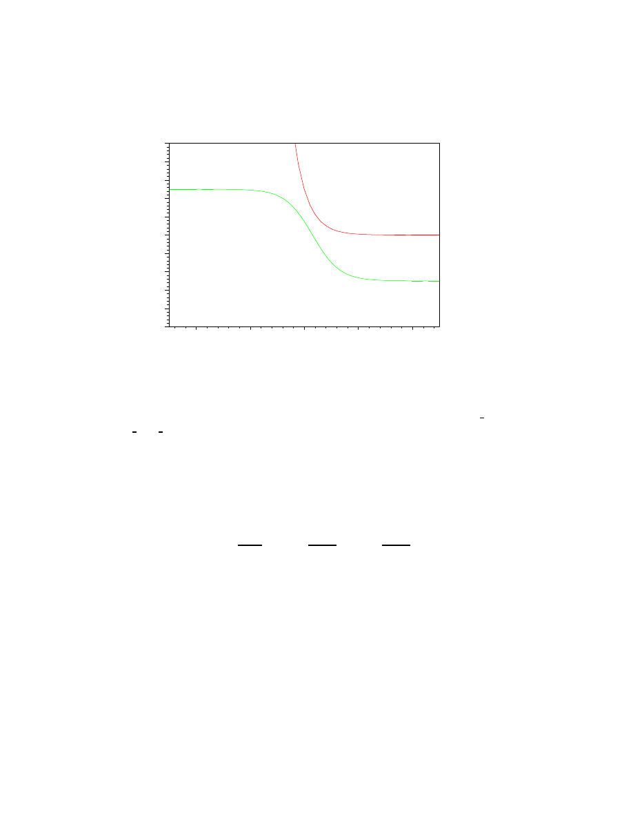
reflection on barrier
–1
–0.8
–0.6
–0.4
–0.2
0
0.2
0.4
0.6
0.8
1
–4
–2
0
2
4
tau
We can see, that the”particle” with initial velocity p
1
= -0.5 (green curve)
is reflected on barrier (red curve) with change of velocity sign. But eq 5,
eq 6, eq 7 results in p
1
+ p
2
= const, p
1
+ p
3
= const therefore
(p
new
)
2
= p
2
+ p
1
- (p
new
)
1
= p
2
+ 2 p
1
, (p
new
)
3
= p
3
+ p
1
- (p
new
)
1
=
p
3
+ 2 p
1
,
t = a b c = e
((1+2 p
1
) τ )
,
and the result is:
a = t
(
−
p1
1+2 p1
)
, b = t
(
p2+2 p1
1+2 p1
)
, c = t
(
p3+2 p1
1+2 p1
)
The following procedure gives a numerical algorithm for iteration of powers
of t.
113

>
iterations := proc(iter,p)
>
p_1_old :=\
>
evalhf( -1/2*p+1/2-1/2*sqrt(-(3*p+1)*(p-1)) );
>
p_2_old :=\
>
evalhf( -1/2*p+1/2+1/2*sqrt(-(3*p+1)*(p-1)) );
>
p_3_old := evalhf( p ):
>
for m from 1 to iter do
>
if(p_1_old<0) then
>
pp := evalhf(1+2*p_1_old):
>
p_1_n := evalhf(-p_1_old/pp):
>
p_2_n := evalhf((p_2_old+2*p_1_old)/pp):
>
p_3_n := evalhf((p_3_old+2*p_1_old)/pp):
>
else fi:
>
if(p_2_old<0) then
>
pp := evalhf(1+2*p_2_old):
>
p_1_n := evalhf((p_1_old+2*p_2_old)/pp):
>
p_2_n := evalhf(-p_2_old/pp):
>
p_3_n := evalhf((p_3_old+2*p_2_old)/pp):
>
else fi:
>
if(p_3_old<0) then
>
pp := evalhf(1+2*p_3_old):
>
p_1_n := evalhf((p_1_old+2*p_3_old)/pp):
>
p_2_n := evalhf((p_2_old+2*p_3_old)/pp):
>
p_3_n := evalhf(-p_3_old/pp):
>
else fi:
>
p_1_old := p_1_n:
>
p_2_old := p_2_n:
>
p_3_old := p_3_n:
>
if m = iter then pts :=\
>
[p_1_old, p_2_old,p_3_old] fi;
>
od:
>
pts
>
end:
>
with(plots):
>
pointplot3d(\
>
{seq(iterations(i,0.6), i=1 ..8)},symbol=diamond,\
>
axes=BOXED,labels=[p_1,p_2,p_3]);
>
pointplot3d(\
>
{seq(iterations(i,0.6), i=7 ..12)},symbol=diamond,\
>
axes=BOXED,labels=[p_1,p_2,p_3]);
114
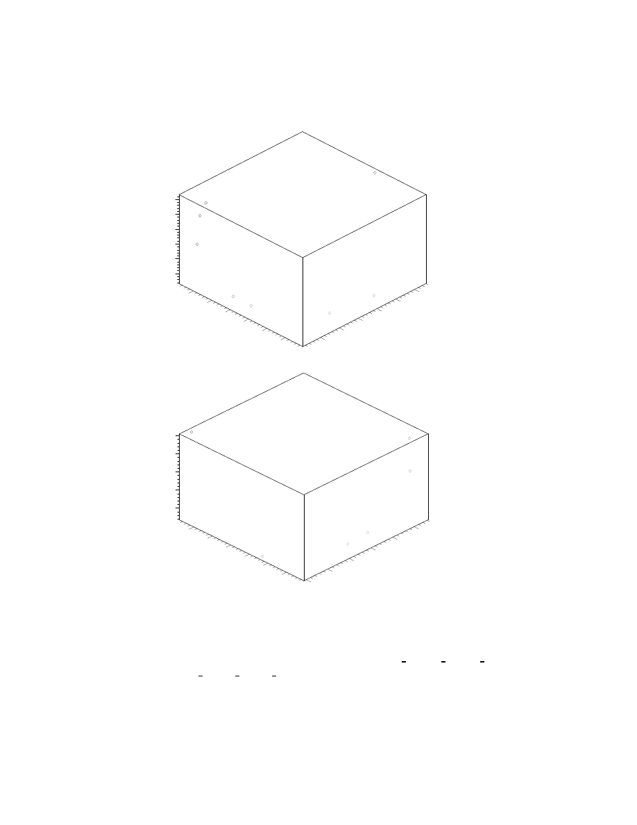
–0.2
0
0.2
0.4
0.6
0.8
p_1
–0.2
0
0.2
0.4
0.6
0.8
p_2
–0.2
0
0.2
0.4
0.6
0.8
p_3
–0.2
0
0.2
0.4
0.6
0.8
p_1
–0.2
0
0.2
0.4
0.6
0.8
p_2
–0.2
0
0.2
0.4
0.6
p_3
One can see, that the evolution has character of switching between different
Kasner’s epochs (all points lie on the section of sphere p 1
2
+ p 2
2
+ p 3
2
=1 by plane p 1 + p 2 + p 3 =1). The negative power of t increases
the corresponding scaling factor if t–>0. In the upper figure the periodical
change of signs takes place between y- and z - directions. The universe
oscillates in these directions and monotone contracts in x-direction (t–>0).
Next the evolution changes (lower figure): x-z oscillations are accompanied
by the contraction in y-direction. The whole picture is the switching between
115
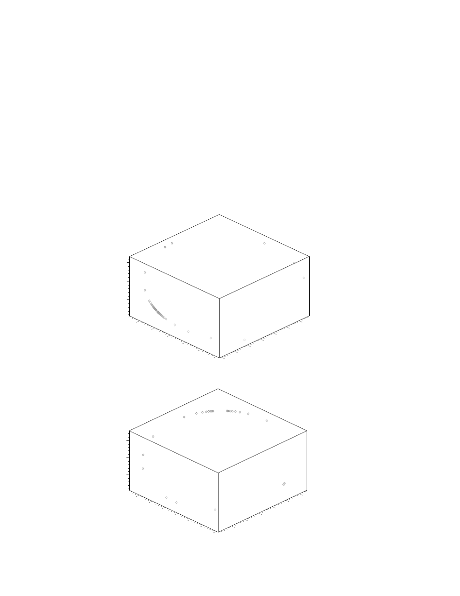
different oscillations as the result of logarithmical approach to singularity. It
is important, that there is the strong dependence on initial conditions that
can cause the chaotical scenario of oscillations:
>
pointplot3d(\
>
{seq(iterations(i,0.601),i=1..100)},symbol=diamond,\
>
axes=BOXED,labels=[p_1,p_2,p_3],\
>
title=‘Kasner’s epochs (I)‘);
>
pointplot3d(\
>
{seq(iterations(i,0.605),i=1..100)},symbol=diamond,\
>
axes=BOXED,labels=[p_1,p_2,p_3],\
>
title=‘Kasner’s epochs (II)‘);
Kasner’s epochs (I)
–0.2
0
0.2
0.4
0.6
0.8
1
p_1
–0.2
0
0.2
0.4
0.6
0.8
p_2
0
0.4
0.8
p_3
Kasner’s epochs (II)
–0.2
0
0.2
0.4
0.6
0.8
p_1
–0.2
0
0.2
0.4
0.6
0.8
1
p_2
0
0.4
0.8
p_3
116
So, we can conclude that the deflection from isotropy changes the scenario
of the universe’s evolution in the vicinity of singularity, so that the dynamics
of the geometry looks like chaotical behavior of the deterministic nonlinear
systems (so-called Mixmaster universe, see [16]).
4.4.2
Inflation
The above-considered standard homogeneous models face the challenge of
so-called horizon. The homogeneity of the universe results from the causal
connection between its different regions. But the distance between these
regions is defined by the time of expansion. Let’s find the maximal distance
of the light signal propagation in the expanding region. As ds
2
= 0 the
accompanying radial coordinate of horizon is
>
r = Int(1/a(t),t=0..t0);# t0 is the age\
>
of the universe
>
#or
>
r = Int(1/y(tau),tau=-t0*H0..0)/(a0*H0);
r =
Z
t0
0
1
a(t)
dt
r =
Z
0
−t0 H0
1
y(τ )
dτ
a0 H0
For instance, in the Einstein-de Sitter model we have
>
int(\
>
subs(y(tau)=1/4*(12*tau+8)^(2/3),1/y(tau)),\
>
tau=-2/3..0)/(a0*H0):# we use the above obtained\
>
expressions for this model
>
simplify( subs(a0=1/4*(12*0+8)^(2/3),%),radical );
2
1
H0
and in the Friedmann-Lemaitre:
117
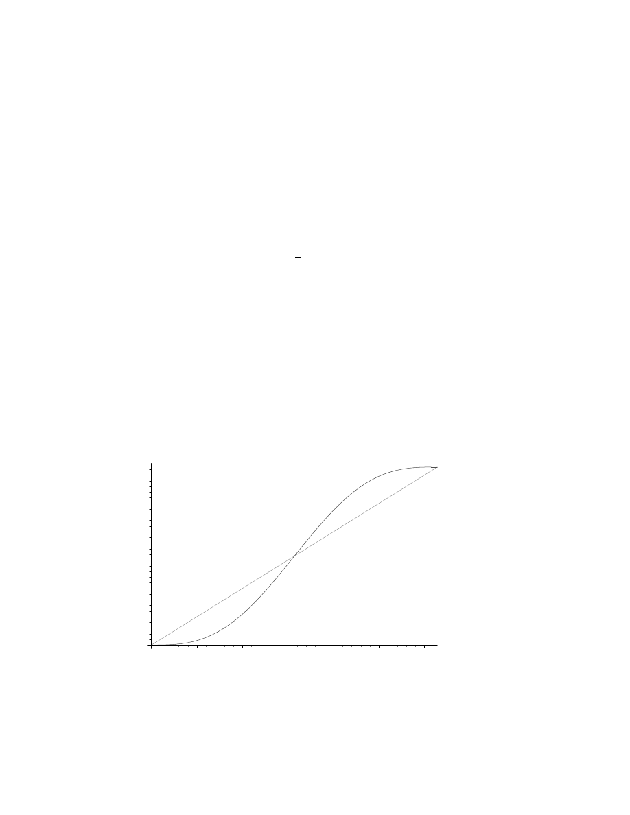
>
int(\
>
subs(y(phi)=Omega[M]*(1-cos(2*phi))/\
>
(2*b),1/2*Omega[M]*(2-2*cos(2*phi))/\
>
(b^(3/2))/y(phi)),phi )/a0/H0;# we use \
>
the above obtained expressions for this model
>
simplify( subs(K=-1,subs(b=-K/a0^2/H0^2,%)),\
>
radical,symbolic);#b=Omega[M]-1=Omega[K] and K=-1\
>
(spherical universe)
2
φ
√
b a0 H0
2 φ
The last example is of interest. The increase of φ from 0 to π /2 corresponds
to expansion of universe up to its maximal radius (see above). At the mo-
ment of maximal expansion the observer can see the photons from antipole
of universe that corresponds to formation of full causal connection:
>
plot([2*phi-sin(2*phi),2*phi],\
>
phi=0..Pi, title=‘age of universe and time of\
>
photon travel (a.u.)‘);
age of universe and time of photon travel (a.u.)
0
1
2
3
4
5
6
0.5
1
1.5
2
2.5
3
phi
This figure shows the age of Friedmann-Lemaitre universe in comparison
with the time of photon propagation from outermost point of universe. For
118
φ < π /2 there are the regions, which don’t connect with us. After this
points there is the causal connection. At the moment of recollapse the pho-
tons complete revolutions around universe.
The different approaches were developed in order to overcome the problem
of horizon (see above considered loitering and Mixmaster models). But the
most popular models are based on the so-called inflation scenario, which can
explain also the global flatness of universe (see, for example, [17], on-line re-
views [18, 19]).
For escape the horizon problem we have to suppose the accelerated expan-
sion with
∂
2
∂t
2
a(t) > 0. As result of this condition, the originally causally
connected regions will expand faster, than the horizon expands. So, we ob-
serve the light from the regions, which was connected at the early stage of
universe’s evolution. In the subsection ”Standard models” we derived from
Einstein equations the energy conservation low basic 2 :
∂2
∂t2
a(t)
a(t)
=
−4 π (p(t) +
ρ(t)
3
) +
Λ
3
This equation demonstrates that in the usual conditions (p > 0) the pressure
is a source of gravitation, but if p < -
ρ
3
( Λ = 0) or Λ > 4 π ρ (p=0) the
repulsion dominates and the expansion is accelerated. As the source of the
repulsion, the scalar ”inflaton” field φ is considered.
Let us introduce the simple Lagrangian for this homogeneous field:
L=-
1
2
∂
∂x
i
φ
∂
∂x
j
φ g
ij
- V ( φ ),
where V is the potential energy. The procedure, which was considered in
first section, allows to derive from this Lagrangian the field equation:
1
√
−g
∂
∂x
i
√
−g g
ij
(
∂
∂x
j
φ) +
∂
∂φ
V = 0.
In the case of flat RW metric this equation results in:
119
>
coord := [t, r, theta, phi]:
>
g_compts :=\
>
array(symmetric,sparse,1..4,1..4):
>
g_compts[1,1] := -1:
>
g_compts[2,2] := a(t)^2:
>
g_compts[3,3]:= a(t)^2*r^2:
>
g_compts[4,4]:= a(t)^2*r^2*sin(theta)^2:
>
g := create([-1,-1], eval(g_compts)):#definition\
>
of flat RW metric
>
d1g:= d1metric(g, coord):
>
g_inverse:= invert( g, ’detg’):
>
Cf1:= Christoffel1 ( d1g ):
>
Cf2:= Christoffel2 ( g_inverse, Cf1 ):
>
det_scal := simplify(\
>
sqrt( -det( get_compts(g) )),radical,symbolic ):
>
g_det_sq :=\
>
create([], det_scal):#sqrt(-g)
>
field :=\
>
create([], phi(t)):#field
>
#calculation of first term in the field equation
>
cov_diff( field, coord, Cf2 ):
>
T := prod(g_inverse,%):
>
contract(T,[2,3]):
>
Tt := prod(g_det_sq,%):
>
Ttt := cov_diff( Tt, coord, Cf2 ):
>
get_compts(%)[1,1]/det_scal:
>
expand(-%):
>
field_eq := % + diff(V(phi),phi) = 0;
field eq := 3
(
∂
∂t
φ(t)) (
∂
∂t
a(t))
a(t)
+ (
∂
2
∂t
2
φ(t)) + (
∂
∂φ
V(φ)) = 0
Now let’s define the energy-momentum tensor for first Einstein equation:
T
ij
= g
ij
L - g
jl
f
x i
∂
∂f
x l
L ,
where f
x i
=
∂
∂x
i
φ . As consequence, ρ = [-
1
2
(
∂
∂t
φ)
2
+ V ( φ )] + (
∂
∂t
φ)
2
=
1
2
(
∂
∂t
φ)
2
+ V ( φ ), and (for i, j = 1,2,3) T
ij
= g
ij
(
1
2
(
∂
∂t
φ)
2
- V ( φ ))
⇒ p
=
1
2
(
∂
∂t
φ)
2
- V ( φ ). Last expression emplies that the necessary condition
p < -
ρ
3
may result from large V.
The dynamics of our system is guided by coupled system of equations:
>
basic_inf_1 :=\
>
K/(a(t)^2)+diff(a(t),t)^2/(a(t)^2) =\
>
8/3*Pi*(1/2*diff(phi(t),t)^2+V(phi));#see above E[1]
>
basic_inf_2 := field_eq;
120
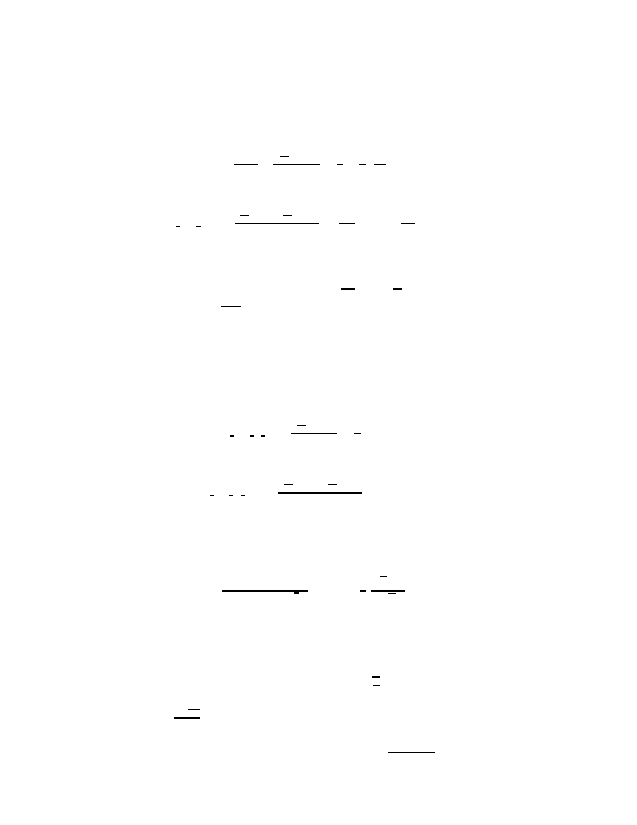
basic inf 1 :=
K
a(t)
2
+
(
∂
∂t
a(t))
2
a(t)
2
=
8
3
π (
1
2
(
∂
∂t
φ(t))
2
+ V(φ))
basic inf 2 := 3
(
∂
∂t
φ(t)) (
∂
∂t
a(t))
a(t)
+ (
∂
2
∂t
2
φ(t)) + (
∂
∂φ
V(φ)) = 0
The meaning of K is considered earlier, here we will suppose K =0 (local
flatness). In the slow-rolling approximation
∂
2
∂t
2
φ(t) , (
∂
∂t
φ(t))
2
–>0 and for
potential V ( φ ) =
m φ
2
2
we have:
>
basic_inf_1_n :=\
>
subs(K=0,K/(a(t)^2)+diff(a(t),t)^2/(a(t)^2)) =\
>
8/3*Pi*m^2*phi(t)^2/2;#see above E[1]
>
basic_inf_2_n :=
op(1,lhs(field_eq)) +\
>
subs(phi=phi(t),expand(subs(V(phi)=m^2*phi^2/2,\
>
op(3,lhs(field_eq)))))=0;
basic inf 1 n :=
(
∂
∂t
a(t))
2
a(t)
2
=
4
3
π m
2
φ(t)
2
basic inf 2 n := 3
(
∂
∂t
φ(t)) (
∂
∂t
a(t))
a(t)
+ m
2
φ(t) = 0
>
dsolve(
{basic_inf_1_n,basic_inf_2_n,\
>
phi(0)=phi0,a(0)=a0
},{phi(t),a(t)}):
>
expand(%);
(
a(t) =
e
(
−1/6 m
2
t
2
)
a0
e
−(2/3 φ0
√
π m
√
3 t)
, φ(t) =
−
1
6
√
3 m t
√
π
+ φ0
)
One can see, that for φ
0
>>1 there is an quasi-exponential expansion (in-
flation) of universe:
a(t)= a
0
e
(H t)
, where H = 2
q
π
3
φ
0
m
When t ˜
2
√
3 π
m
φ
0
the regime of slow rolling ends and the potential energy
of inflaton field converts into kinetic form that causes the avalanche-like
creation of other particles from vacuum (so-called ”reheating”). Only at
121

this moment the scenario become similar to Big Bang picture. What is the
size of universe after inflation?
>
a(t)=subs(\
>
{H=2*sqrt(Pi/3)*phi[0]*m,t=2*sqrt(3*Pi)/m*phi[0]},\
>
a[0]*exp(H*t));
a(t) = a
0
e
(4 π φ
0
2
)
If at the beginning of inflation the energy and size of universe are defined by
Plank density and length, then m
2
(φ
2
)
0
˜1, a
0
˜10
(
−33)
cm. The necessary
value of m ˜10
(
−6)
is constrained from the value of fluctuation of back-
ground radiation ( ˜10
(
−5)
). As result a ˜ 10
(
−33)
e
(
4 π
m2
)
= 10
(
−33)
e
(4 π 10
12
)
cm , that is much larger of the observable universe. This is the reason why
observable part of universe is flat, homogeneous and isotropic.
Let’s return to basic inf 2. The reheating results from oscillation of inflaton
field around potential minimum that creates new boson particles. The last
damps the oscillations that can be taking into consideration by introducing
of dumping term in basic inf 2 :
>
reh_inf :=\
>
3*diff(phi(t),t)*H+Gamma*diff(phi(t),t) +\
>
diff(phi(t),‘$‘(t,2)) = -m^2*phi(t);
reh inf := 3 (
∂
∂t
φ(t)) H + Γ (
∂
∂t
φ(t)) + (
∂
2
∂t
2
φ(t)) =
−m
2
φ(t)
Here H is the Hubble constant, Γ is the decay rate, which is defined by
coupling with material boson field. When H > Γ , there are the coherent
oscillations:
>
dsolve(subs(Gamma=0,reh_inf),phi(t));
>
diff(%,t);
φ(t) = C1 e
(
−1/2 (3 H+
√
(3 H
−2 m) (3 H+2 m)) t)
+
C2 e
(
−1/2 (3 H−
√
(3 H
−2 m) (3 H+2 m)) t)
122

∂
∂t
φ(t) = C1 (
−
3
2
H
−
1
2
%1) e
(
−1/2 (3 H+%1) t)
+
C2 (
−
3
2
H +
1
2
%1) e
(
−1/2 (3 H−%1) t)
%1 :=
p
(3 H
− 2 m) (3 H + 2 m)
The last expression demonstrates the decrease of energy density via time
increase ( ρ ˜ (
∂
∂t
φ)
2
) and, as result, the decrease of H (see basic inf 1 ).
This leads to H < Γ , that denotes the reheating beginning.
In the conclusion of this short and elementary description it should be noted,
that the modern inflation scenarios modify the standard model essentially.
The Universe here looks like fractal tree of bubbles-universes, inflating and
recollapsing foams, topological defects etc. The main features of this picture
wait for thorough investigations.
5
Conclusion
Our consideration was brief and I omitted some important topics like per-
turbation theory for black holes and cosmological models, Penrose diagrams
and conformal mappings for investigation of causal structure, gravitational
waves etc. But I suppose to advance this worksheet hereafter.
References
[1] see http://grtensor.phy.queensu.ca
[2] Sommerfeld A. Lectures on theoretical physics, v. 3, Academic Press,
NY, 313-315 (1952).
[3] Kai-Chia Cheng. A simple calculation of the perihelion Mercury from
the principle of equivalence. Nature (Lond.), v. 155, 574 (1945).
[4] N.T. Roseveare, Mercury’s perihelion from Le Verrier to Einstein,
Clarendon Press - Oxford (1982).
[5] J. L. Synge, Relativity: the general theory, Amsterdam (1960).
[6] E. T. Whittaker, G. N. Watson, A course of modern analysis, Cam-
bridge (1927).
[7] C. W. Misner, K. S. Thorne, J. A. Wheeler, Gravitation, San Francisco
(1973).
123
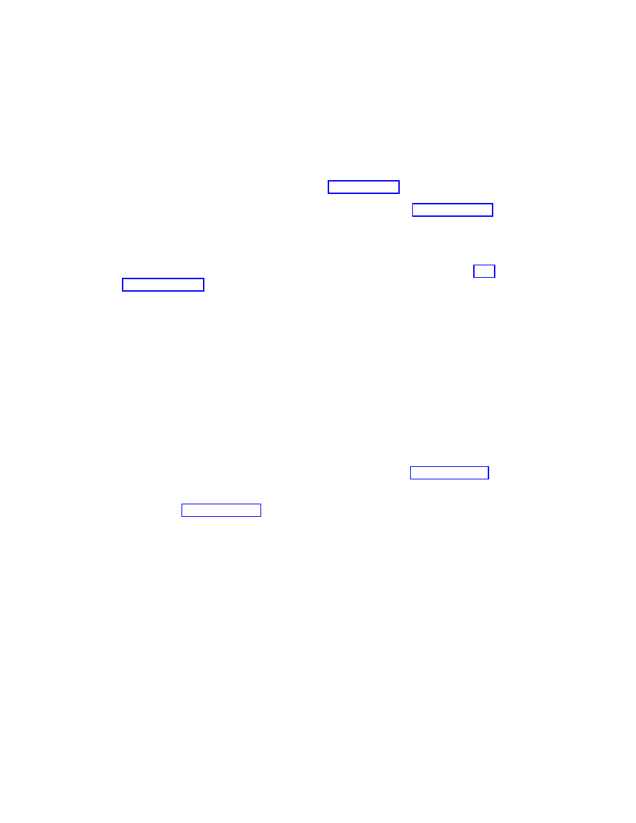
[8] V. Frolov, I. Novikov, Physics of Black Holes, Kluwer, Dordrecht (1998).
[9] W. Pauli, Theory of relativity, Pergamon Press (1958).
[10] P.K. Townsend, Black Holes, arXiv: gr-gc/9707012.
[11] J. Garcia-Bellido, Astrophysics and cosmology, arXiv: hep-ph/0004188.
[12] P.J.E. Peebles, Principles of physical cosmology, Prinston Univ. Press
(1993).
[13] P. B. Pal, Determination of cosmological parameters, arXiv: hep-
[14] Ya.B. Zel’dovich, I.D. Novikov, Relativistic Astrophysics, V. 2: The
structure and evolution of the universe, The university of Chicago Press,
Chicago (1983).
[15] L.D. Landau, E.M. Lifshitz, The classical theory of fields, Pergamon
Press, Oxford (1962).
[16] J. Wainwright, C.F.R. Ellis, eds., Dynamical systems in cosmology,
Cambridge University press, Cambridg (1997).
[17] A.D. Linde, Particle physics and inflationary cosmology, Harwood aca-
demic press, Switzerland (1990).
[18] A. Linde, Lectures on inflationary cosmology, arXiv: hep-th/9410082.
[19] R.H. Brandenberger, Inflationary cosmology: progress and problems,
arXiv: hep-ph/9910410.
124
Wyszukiwarka
Podobne podstrony:
Introduction to Differential Geometry and General Relativity
Introduction to the MOSFET and MOSFET Inverter(1)
An Introduction to USA 5 Science and Technology
An Introduction to USA 2 Geographical and Cultural Regions of the USA
Graham Cole & Michael Schluter FROM PERSONALISM TO RELATIONISM COMMONALITIES AND DISTINCTIVES
Bruzzo U Introduction to Algebraic Topology and Algebraic Geometry
Baker A Introduction To p adic Numbers and p adic Analysis
Introduction to language acquisition and language learning
PP BH&C 0 1 Introduction to the History and Culture of the B
Taylor; Introduction To The Philosophy And Writings Of Plato
SCHAFER, Christian The Philosophy of Dionysius the Areopagite an introduction to the structure and
An Introduction to Statistical Inference and Data Analysis M Trosset (2001) WW
Zizek, Slavoj Looking Awry An Introduction to Jacques Lacan through Popular Culture
Introduction to Lagrangian and Hamiltonian Mechanics BRIZARD, A J
Introduction to CPLD and FPGA Design
Introduction to Mechatronics and Measurement Systems
Introduction to Prana and Pranic Healing – Experience of Breath and Energy (Pran
An Introduction to USA 1 The Land and People
więcej podobnych podstron