
Generalized functions
in mathematical physics.
Main ideas and concepts
A.S. Demidov


Contents
vii
xi
Introduction to problems of mathematical physics
1
Temperature at a point? No! In volumes contracting to
1
The notion of δ-sequence and δ-function
4
Some spaces of smooth functions. Partition of unity
6
10
11
19
The Ostrogradsky–Gauss formula. The Green formulae
28
31
40
45
Simplest hyperbolic equations. Generalized Sobolev
solutions
46
distribution theory (generalized function in the
sense of L. Schwartz)
59
59
63
66
Generalized functions with a point support. The Borel
theorem
68
of generalized functions (distributions by
72
v

vi
CONTENTS
. Pseudodifferential operators
81
The Fourier series and the Fourier transform. The
spaces S and S
81
The Fourier–Laplace transform. The Paley–Wiener
theorem
94
Fundamental solutions. Convolution
99
102
On pseudodifferential operators (PDO)
106
111
A new approach to the theory
of generalized functions
(Yu.V. Egorov)
129
137
141

Preface
Presently, the notion of function is not as finally crystallized
and definitely established as it seemed at the end of the 19th cen-
tury; one can say that at present this notion is still in evolution,
and that the dispute concerning the vibrating string is still going on
only, of course, in different scientific circumstances, involving other
personalities and using other terms.
Luzin N.N. (1935) [42]
It is symbolic that in that same year of 1935, S.L. Sobolev, who
was 26 years old that time, submitted to the editorial board of the
journal “Matematicheskiy sbornik” his famous work [61] and pub-
lished at the same time its brief version in “Doklady AN SSSR” [60].
This work laid foundations of a completely new outlook on the con-
cept of function, unexpected even for N.N. Luzin — the concept of
a generalized function (in the framework of the notion of distribu-
tion introduced later). It is also symbolic that the work by Sobolev
was devoted to the Cauchy problem for hyperbolic equations and, in
particular, to the same vibrating string.
In recent years Luzin’s assertion that the discussion concern-
ing the notion of function is continuing was confirmed once again,
and the stimulus for the development of this fundamental concept
of mathematics is, as it was before, the equations of mathematical
physics (see, in particular, Addition written by Yu.V. Egorov and
[10, 11, 16, 17, 18, 32, 49, 67]). This special role of the equa-
tions of mathematical physics (in other words, partial differential
equations directly connected with natural phenomena) is explained
by the fact that they express the mathematical essence of the funda-
mental laws of the natural sciences and consequently are a source and
stimulus for the development of fundamental mathematical concepts
and theories.
vii
viii
PREFACE
The crucial role in appearance of the theory of generalized func-
tions (in the sense the theory of distributions) was played by J. Ha-
damard, K.O. Friedrichs, S. Bochner, and especially to L. Schwartz,
who published, in 1944–1948, a series of remarkable papers concern-
ing the theory of distributions, and in 1950–1951 a two-volume book
[54], which immediately became classical. Being a masterpiece and
oriented to a wide circle of specialists, this book attracted the at-
tention of many people to the theory of distributions. The huge
contribution to its development was made by such prominent math-
ematicians as I.M. Gel’fand, L. H¨
ormander and many others. As a
result, the theory of distributions has changed all modern analysis
and first of all the theory of partial differential equations. Therefore,
the foundations of the theory of distributions became necessary for
general education of physicists and mathematicians. As for students
specializing in the equations of mathematical physics, they cannot
even begin any serious work without knowing the foundations of the
theory of distributions.
Thus, it is not surprising that a number of excellent monographs
and textbooks (see, for example, [12, 22, 23, 25, 31, 40, 44, 54,
57, 59, 62, 68, 69]) are devoted to the equations of mathematical
physics and distributions. However, most of them are intended for
rather well prepared readers. As for this small book, I hope that it
will be clear even to undergraduates majoring in physics and math-
ematics and will serve to them as starting point for a deeper study
of the above-mentioned books and papers.
In a nutshell the book gives an interconnected presentation of
a some basic ideas, concepts, results of the theory of generalized
functions (first of all, in the framework of the theory of distributions)
and equations of mathematical physics.
Chapter 1 acquaints the reader with some initial elements of the
language of distributions in the context of the classical equations
of mathematical physics (the Laplace equation, the heat equation,
the string equation). Here some basic facts from the theory of the
Lebesgue integral are presented, the Riesz spaces of integrable func-
tions are introduced. In the section devoted to the heat equation,
the student of mathematics can get familiar with the method of
dimensionality and similarity, which is not usually included in the
university program for mathematicians, but which is rather useful on
the initial stage of study of the problems of mathematical physics.

PREFACE
ix
Chapter 2 is devoted to the fundamentals of the theory of distri-
butions due to L. Schwartz. Section 16 is the most important. The
approach to some topics can also be interesting for the experts.
Chapter 3 acquaints the reader with some modern tools and
methods for the study of linear equations of mathematical physics.
The basics of the theory of Sobolev spaces, the theory of pseudodif-
ferential operators, the theory of elliptic problems (including some
elementary results concerning the index of elliptic operators) as well
as some other problems connected in some way with the Fourier
transform (ordinary functions and distributions) are given here.
Now I would like to say a few words concerning the style of the
book. A part of the material is given according to the scheme: defini-
tion — theorem — proof. This scheme is convenient for presenting
results in clear and concentrated form. However, it seems reason-
able to give a student the possibility not only to study a priori given
definitions and proofs of theorems, but also to discover them while
considering the problems involved. A series of sections serves this
purpose. Moreover, a part of the material is given as exercises and
problems. Thus, reading the book requires, in places, a certain ef-
fort. However, the more difficult problems are supplied with hints
or references. Problems are marked by the letter P (hint on Parking
for the solution of small Problems).
The importance of numerous notes is essentially connected with
a playful remark by V.F. D’yachenko: “The most important facts
should be written in notes, since only those are read”. The notes are
typeset in a small font and located in the text immediately after the
current paragraph.
I am very grateful to Yu.V. Egorov, who kindly agreed to write
Addendum to the book. I would also like to acknowledge my grati-
tude to M.S. Agranovich, A.I. Komech, S.V. Konyagin, V.P. Palam-
odov, M.A. Shubin, V.M. Tikhomirov, and M.I. Vishik for the useful
discussions and critical remarks that helped improve the manuscript.
I am also thankful to E.V. Pankratiev who translated this book and
produced the CRC.
While preparing this edition, some corrections were made and
the detected misprints have been corrected.
A.S. Demidov

Notation
N = {1, 2, 3, . . . }, Z = {0, ±1, ±2, . . . } and Z
+
= {0, ±1, ±2, . . . } are
the sets of natural numbers, integers and non-negative integers.
X × Y is the Cartesian product of the sets X and Y , X
n
= X
n−1
× X.
i =
√
−1 is the imaginary unit (“dotted i”).
◦
ı = 2πi the imaginary 2π (“i with a circle”).
R
n
and C
n
are n-dimensional Euclidean and complex spaces; R = R
1
,
C = C
1
3 z = x + iy, where x = <z ∈ R and y = =z ∈ R.
x < y, x ≤ y, x > y, x ≥ y are the order relations on R.
a 1 means the a sufficiently large.
{x ∈ X | P } is the set of elements which belong to X and have a
property P .
]a, b] = {x ∈ R | a < x ≤ b}; [a, b], ]a, b[ and [a, b[ are defined similarly.
{a
n
} is the sequence {a
n
}
∞
n=1
= {a
1
, a
2
, a
3
, . . . }.
f : X 3 x 7→ f (x) ∈ Y is the mapping f : X → Y , putting into
correspondence to an element x ∈ X the element f (x) ∈ Y .
1
A
is the characteristic function of the set A, i.e. 1
A
= 1 in A and
1
A
= 0 outside of A.
arccot α =
π
2
− arctan α.
x → a means that the numerical variable x converges (tends) to a.
=⇒ means “it is necessary follows”.
⇐⇒ means “if and only if” (“iff”), i.e an equivalence.
A b Ω means A is compactly embedded in Ω (see Definition 3.2).
C
m
(Ω), C
m
b
(Ω), C
m
( ¯
Ω), P C
m
(Ω), P C
m
b
(Ω), C
m
0
(Ω), C
m
0
( ¯
Ω) see Defi-
nition 3.1 (for 0 ≤ m ≤ ∞).
L
p
(Ω), L
∞
(Ω), L
p
loc
(Ω) see Definitions 9.1, 9.9, 9.15.
D
[
(Ω), D
#
(Ω), D(Ω), D
0
(Ω) see Definitions 12.2, 13.1, 16.7, 16.9.
E(Ω), E
0
(Ω) see P.16.13.
S(R
n
), S
0
(R
n
) see Definitions 17.10, 17.18.
xi


CHAPTER 1
Introduction to problems of
mathematical physics
1. Temperature at a point? No! In volumes contracting to
the point
Temperature. We know this word from our childhood. The tem-
perature can be measured by a thermometer. . . This first impression
concerning the temperature is, in a sense, nearer to the essence than
the representation of the temperature as a function of a point in
space and time. Why? Because the concept of the temperature as
a function of a point arose as an abstraction in connection with the
conception of continuous medium. Actually, a physical parameter
of the medium under consideration (for instance, its temperature)
is first measured by a device in a “large” domain containing the
fixed point ξ, then using a device with better resolution in a smaller
domain (containing the same point) an so on. As a result, we ob-
tain a (finite) sequence of numbers {a
1
, . . . , a
M
} — the values of the
physical parameter in the sequence of embedded domains contain-
ing the point ξ. We idealize the medium considered, by assuming
that the construction of the numerical sequence given above is for
an infinite system of domains containing the point ξ and embedded
in each other. Then we obtain an infinite numerical sequence {a
m
}.
If we admit (this is the essence of the conception of the continuous
medium
1)
, that such a sequence exists and has a limit (which does
not depend on the choice of the system of embedded in each other
domains), then this limit is considered as the value of the physical
parameter (for instance, temperature) of the considered medium at
the point ξ.
1)
In some problems of mathematical physics, first of all in nonlin-
ear ones, it is reasonable (see, for example, [10, 11, 16, 18, 32, 49]) to
1

2
1. INTRODUCTION TO PROBLEMS OF MATHEMATICAL PHYSICS
consider a more general conception of the continuous medium in which a
physical parameter (say, temperature, density, velocity. . . ) is character-
ized not by the values measured by one or another set of “devices”, in
other words, not by a functional of these “devices”, but a “convergent”
sequence of such functionals which define, similarly to nonstandard anal-
ysis [5, 13, 73], a thin structure of a neighbourhood of one or another
point of continuous medium.
Thus, the concept of continuous medium occupying a domain
2)
Ω, assumes that the numerical characteristic f of a physical param-
eter considered in this domain (i.e. in Ω) is a function in the usual
sense: a mapping from the domain Ω into the numerical line (i.e. into
R or into C). Moreover, the function f has the following property:
hf, ϕ
ξ
m
i = a
m
,
m = 1, . . . , M.
(1.1)
Here, a
m
are the numbers introduced above, and the left-hand side
of (1.1), which is defined
3)
by the formula hf, ϕ
ξ
i =
R f (x)ϕ
ξ
(x)dx,
represents the “average” value of the function f , measured in the
neighbourhood of the point ξ ∈ Ω by using a “device”, which will
be denoted by h·, ϕ
ξ
i. The “device” has the resolving power, that
is determined by its “device function” (or we may also say “test
function”) ϕ
ξ
: Ω → R. This function is normed:
R ϕ
ξ
(x)dx = 1.
2)
Always below, if the contrary is not said explicitly, the domain Ω
is an open connected set in R
n
, where n > 1, with a sufficiently smooth
(n − 1)-dimensional boundary ∂Ω.
3
) Integration of a function g over a fixed (in this context) domain
will be often written without indication of the domain of integration, and
sometimes simply in the form
R g.
Let us note that more physical are “devices”, in which ϕ
ξ
has
the form of a “cap” in the neighbourhood of the point ξ, i.e. ϕ
ξ
(x) =
ϕ(x − ξ) for x ∈ Ω, where the function ϕ : R
n
3 x = (x
1
, . . . , x
n
) 7−→
ϕ(x) ∈ R has the following properties:
ϕ ≥ 0,
Z
ϕ = 1,
ϕ = 0 outside the ball {x ∈ R
n
|x| ≡
q
x
2
1
+ · · · + x
2
n
≤ ρ}.
(1.2)
Here, ρ ≤ 1 is such that {x ∈ Ω
|x − ξ| < ρ} ⊂ Ω. Often one
can assume that the “device” measures the quantity f uniformly

1. TEMPERATURE AT A POINT? NO! IN VOLUMES
3
in the domain ω ∈ Ω. In this case, ϕ = 1
ω
/|ω|, where 1
ω
is the
characteristic function of the domain ω (i.e. 1
ω
= 1 in ω and 1
ω
= 0
outside ω), and |ω| is the volume of the domain ω (i.e. |ω| =
R 1
ω
). In
particular, if Ω = R
n
and ω = {x ∈ R
n
|x| < α}, then ϕ(x) = δ
α
(x),
where
δ
α
(x) =
(
α
−n
/|B
n
|
f or |x| ≤ α,
0
f or |x| > α,
(1.3)
and |B
n
| is the volume of the unit ball B
n
in R
n
.
1.1.P. It is well known that |B
2
| = π and |B
3
| = 4π/3. Try to
calculate |B
n
| for n > 3. We shall need it below.
Hint. Obviously, |B
n
| = σ
n
/n, where σ
n
is the area of the
surface of the unit (n − 1)-dimensional sphere in R
n
, since |B
n
| =
R
1
0
r
n−1
σ
n
dr. If the calculation of σ
n
for n > 3 seems to the reader
difficult or noninteresting, he can read the following short and unex-
pectedly beautiful solution.
Solution. We have
∞
Z
−∞
e
−t
2
dt
!
n
=
Z
R
n
e
−|x|
2
dx =
∞
Z
0
e
−r
2
r
n−1
σ
n
dr = (σ
n
/2) · Γ(n/2),
(1.4)
where Γ(·) is the Euler function defined by the formula
Γ(λ) =
∞
Z
0
t
λ−1
e
−t
dt, where <λ > 0.
(1.5)
For n = 2 the right-hand side of (1.4) is equal to π. Therefore,
∞
Z
−∞
e
−t
2
dt =
√
π.
(1.6)
Thus, σ
n
= 2π
n/2
Γ
−1
(n/2). By taking n = 3, we obtain 2Γ(3/2) =
√
π. By virtue of the remarkable formula Γ(λ + 1) = λ · Γ(λ), (ob-
tained from (1.5) by integration by parts and implying Γ(n+1) = n!),

4
1. INTRODUCTION TO PROBLEMS OF MATHEMATICAL PHYSICS
this implies that Γ(1/2) =
√
π. Now we get that
σ
2n
=
2π
n
(n − 1)!
,
σ
2n+1
=
2π
n
(n − 1/2) · (n − 3/2) · · · · · 3/2 · 1/2
.
(1.7)
2. The notion of δ-sequence and δ-function
In the preceding section the idea was indicated that the defini-
tion of a function f : Ω → R (or of a function f : Ω → C) as a
mapping from a domain Ω ⊂ R
n
into R (or into C) is equivalent to
determination of its “average values”:
hf, ϕi =
Z
Ω
f (x)ϕ(x) dx,
ϕ ∈ Φ,
(2.1)
where Φ is a sufficiently “rich” set of functions on Ω. A sufficiently
general result concerning this fact is given in Section 10. Here, we
prove a simple but useful lemma.
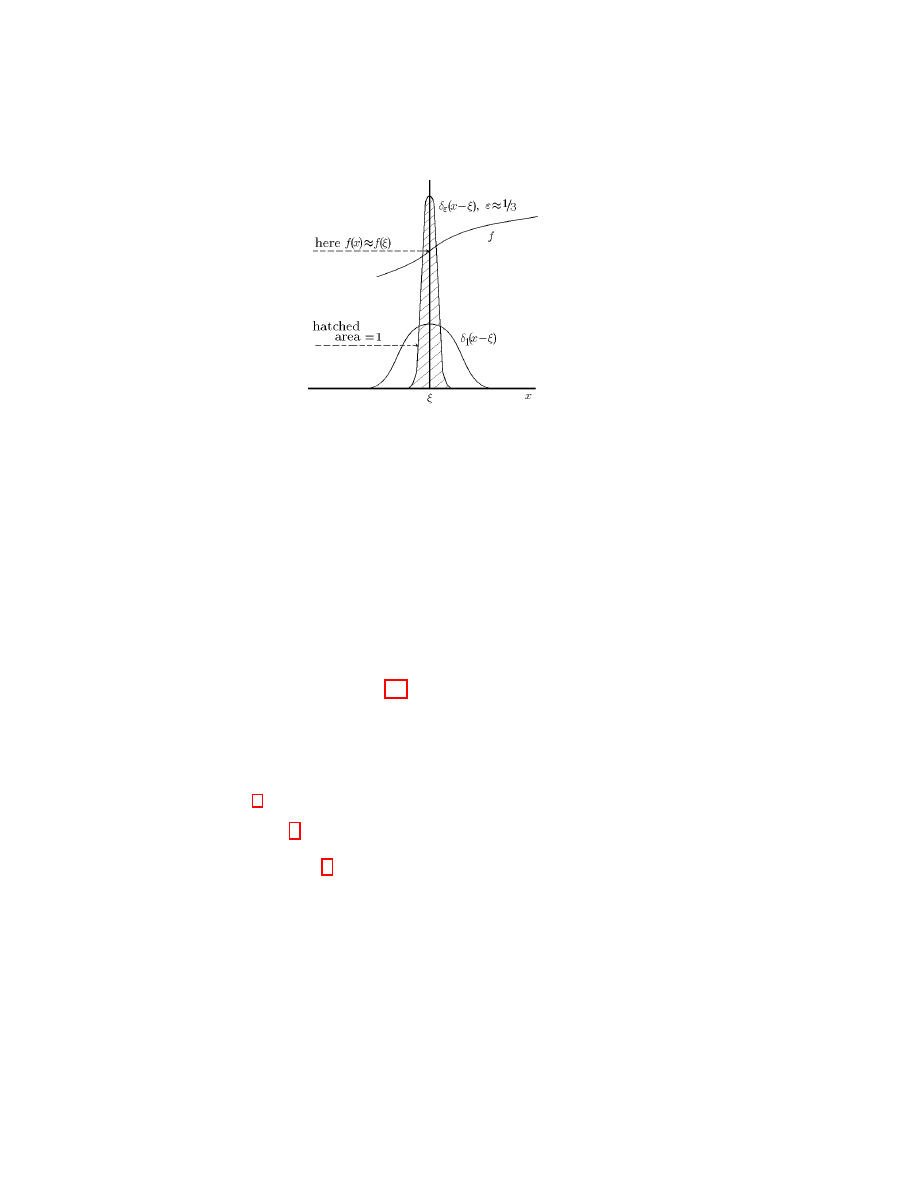
Preliminary, we introduce for
ε ∈]0, 1] the function δ
ε
: R
n
→ R by the formula
δ
ε
(x) = ϕ(x/ε)/ε
n
, ϕ ≥ 0,
Z
ϕ = 1, ϕ = 0 outside B
n
.
(2.2)
Let us note that for 1/ε 1 we have
Z
R
n
δ
ε
(x) dx =
Z
Ω
δ
ε
(x − ξ) dx = 1,
ξ ∈ Ω.
2.1. Lemma. Let f ∈ C(Ω), i.e. f is continuous in Ω ⊂ R
n
.
Then
f (ξ) = lim
ε→0
Z
Ω
f (x)δ
ε
(x − ξ) dx,
ξ ∈ Ω,
(2.3)
i.e. the function f can be recovered by the family of “average values”
Z
f (x) · δ
ε
(x − ξ)dx
ξ∈Ω, ε>0
.
Proof. For any η > 0, there exists ε > 0 such that |f (x) −
f (ξ)| ≤ η if |x − ξ| ≤ ε. Therefore,
2. THE NOTION OF δ-SEQUENCE AND δ-FUNCTION
5
Z
Ω
f (x)δ
(x − ξ) dx
− f (ξ)
=
Z
Ω
(f (x) − f (ξ))δ
(x − ξ) dx
≤
Z
|x−ξ|≤
|f (x) − f (ξ)|δ
(x − ξ) dx
≤ η
Z
|x−ξ|≤
δ
(x − ξ) dx = η.
2.2. Definition. Let Φ be a subspace of the space C(Ω) and
ξ ∈ Ω. A sequence {δ
(x − ξ), x ∈ Ω}
∈R,→0
of functions x 7−→
δ
(x − ξ) such that equality (2.3) holds for any f ∈ C(Ω) (for any
f ∈ Φ) is called δ-sequence (on the space
1)
Φ) concentrated near the
point ξ. The last words are usually skipped.
1)
The notion of δ-sequence on the space Φ allow to obtain a series of
rather important results. Some of them are mentioned at the beginning
of Section 4.
In Section 4 some examples of δ-sequences on one or another
subspace Φ ⊂ C(Ω) are given. Important examples of such sequences
are given in Section 3.

6
1. INTRODUCTION TO PROBLEMS OF MATHEMATICAL PHYSICS
2.3. Definition. A linear functional
2)
δ
ξ
defined on the space
C(Ω) by the formula
δ
ξ
: C(Ω) 3 f 7−→ f (ξ) ∈ R (or C), ξ ∈ Ω,
(2.4)
is called the δ-function, or the Dirac function concentrated at the
point ξ.
2)
A (linear) functional on a (linear) space of functions is defined as
a (linear) mapping from this functional space into a number set.
Often one writes δ-function (2.4) in the form δ(x − ξ) and its
action on a function f ∈ C(Ω) writes (see formula (1.1)) in the form
hf (x), δ(x − ξ)i = f (ξ)
or
hδ(x − ξ), f (x)i = f (ξ).
(2.5)
The following notation is also used: hf, δ
ξ
i = f (ξ) or hδ
ξ
, f i =
f (ξ). The Dirac function can be interpreted as a measuring instru-
ment at a point (a “thermometer” measuring the “temperature” at
a point). If ξ = 0, then we write δ or δ(x).
3. Some spaces of smooth functions. Partition of unity
The spaces of smooth functions being introduced in this section
play very important role in the analysis. In particular, they give
examples of the space Φ in the “averaging” formula (2.1).
3.1. Definition. Let Ω be an open set in R
n
, ¯
Ω the closure of
Ω in R
n
, and m ∈ Z
+
, i.e., m is a non-negative integer. Then
1)
1)
If m = 0, then the index m in the designation of the spaces defined
below is usually omitted.
3.1.1. C
m
(Ω) (respectively, C
m
b
(Ω)) is the space! C
m
(Ω) of m-
times continuously differentiable (respectively, with bounded
derivatives) functions ϕ : Ω → C, i.e., such that the func-
tion ∂
α
ϕ is continuous (and respectively, bounded) in Ω for
|α| ≤ m. Here and below
∂
α
ϕ(x) =
∂
|α|
ϕ(x)
∂x
α
1
1
. . . ∂x
α
n
n
, |α| = α
1
+· · ·+α
n
, α
j
∈ Z
+
= {0, 1, 2, . . . }.
The vector α = (α
1
, . . . , α
n
) is called a multiindex.

3. SOME SPACES OF SMOOTH FUNCTIONS. PARTITION OF UNITY
7
3.1.2. C
m
( ¯
Ω) = C
m
(R
n
)
Ω
, i.e.
2)
C
m
( ¯
Ω) is the restriction of the
space C
m
(R
n
) to Ω. This means that ϕ ∈ C
m
( ¯
Ω) ⇐⇒
there exists a function ψ ∈ C
m
(R
n
) such that ϕ(x) = ψ(x)
for x ∈ Ω.
2)
The space C
m
( ¯
Ω), in general, does not coincide with
the space of functions m-times continuously differentiable up to
the boundary. However, they coincide, if the boundary of the
domain is sufficiently smooth.
3.1.3. P C
m
(Ω) (respectively, P C
m
b
(Ω)) is the space of functions
m-times piecewise continuously differentiable (and respec-
tively, bounded ) in Ω; this means that ϕ ∈ P C
m
(Ω) (re-
spectively, ϕ ∈ P C
m
b
(Ω)) if and only if the following two
conditions are satisfied. First, ϕ ∈ C
m
(Ω \ K
0
) (respec-
tively, ϕ ∈ C
m
b
(Ω \ K
0
)) for a compact
3)
K
0
⊂ Ω. Second,
for any compact K ⊂ ¯
Ω there exists a finite number of do-
mains Ω
j
⊂ Ω, j = 1, . . . , N , each of them is an intersection
of a finite number of domains with smooth boundaries, such
that K ⊂
S
N
j=1
¯
Ω
j
and ϕ
ω
∈ C
m
(¯
ω) for any connected
component ω of the set
N
S
j=1
Ω
j
\
N
S
j=1
∂Ω
j
!
.
3)
A set K ⊂ R
n
is called compact , if K is bounded and
closed.
3.1.4. The support of a function ϕ ∈ C(Ω), denoted by supp ϕ,
is the complement in Ω of the set {x ∈ Ω | ϕ(x) 6= 0}.
In other words, supp ϕ is the smallest set closed in Ω such
that the function ϕ vanishes outside this set.
3.1.5. C
m
0
( ¯
Ω) = {ϕ ∈ C
m
( ¯
Ω) | supp ϕ is a compact}.
3.1.6. C
m
0
(Ω) = {ϕ ∈ C
m
0
( ¯
Ω) | supp ϕ ⊂ Ω}.
3.1.7. C
∞
(Ω) =
T
m
C
m
(Ω),. . . , C
∞
0
(Ω) =
T
m
C
m
0
(Ω).
3.1.8. If ϕ ∈ C
m
0
(Ω) (or ϕ ∈ C
∞
0
(Ω)) and supp ϕ ⊂ ω, where ω
is a subdomain of Ω, then the function ϕ is identified with
its restriction to ω. In this case we write: ϕ ∈ C
m
0
(ω) (or
ϕ ∈ C
∞
0
(ω)).
3.2. Definition. We say that a set A is compactly embedded in
Ω, if ¯
A is a compact and ¯
A ⊂ Ω. In this case we write A b Ω.
8
1. INTRODUCTION TO PROBLEMS OF MATHEMATICAL PHYSICS
Obviously, C
m
0
(Ω) = {ϕ ∈ C
m
(Ω) | supp ϕ b Ω}, and
C
m
0
(Ω) ( C
m
0
( ¯
Ω) ( C
m
( ¯
Ω) ( C
m
(Ω) ( P C
m
(Ω),
where the first inclusion and the third one should be replaced by =,
if Ω = R
n
.
3.3. Example.
C
m
0
(R
n
) 3 ϕ : x 7−→ ϕ(x) =
(
(1 − |x|
2
)
m+1
f or |x| < 1,
0
f or |x| ≥ 1.
3.4. Example.
C
∞
0
(R
n
) 3 ϕ : x 7−→ ϕ(x) =
(
exp(1/(|x|
2
− 1))
f or |x| < 1,
0
f or |x| ≥ 1.
3.5. Example (A special case of (2.2)). Let > 0. we set
ϕ
(x) = ϕ(x/),
(3.1)
where ϕ is the function from Example 3.4. Then the function
δ
: x 7−→ ϕ
(x)/
Z
R
n
ϕ
(x)dx,
x ∈ R
n
,
(3.2)
belongs to C
∞
0
(R
n
) and, moreover,
δ
(x) ≥ 0, ∀x ∈ R
n
, δ
(x) = 0 f or |x| > ,
Z
R
n
δ
(x) dx = 1. (3.3)
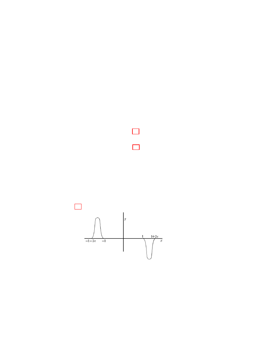
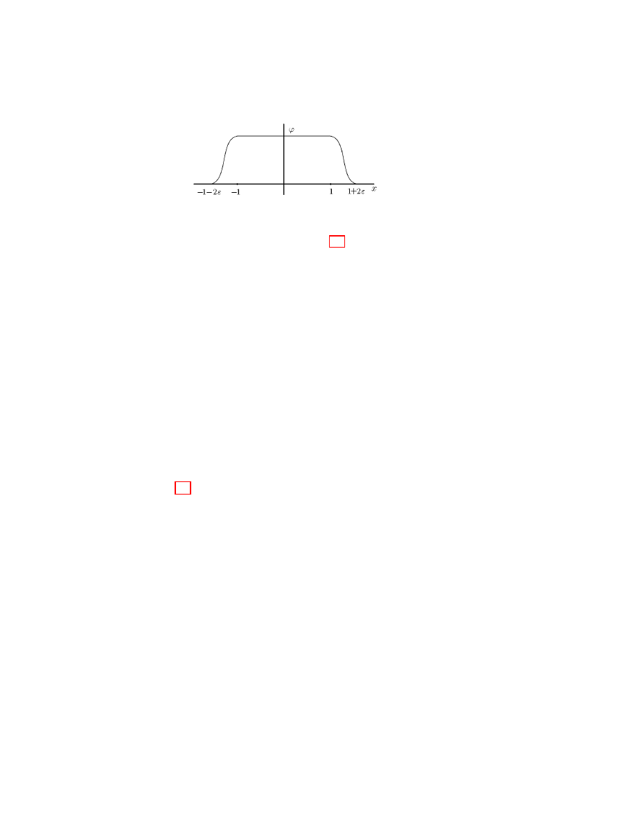
3.6. Example. Let x ∈ R, ϕ : x 7−→ ϕ(x) =
R
x
−∞
g(τ )dτ , where
(see Fig.) g(−x) = −g(x) and g(x) = δ
(x + 1 + ) for x < 0 (δ
satisfies (3.3)).
3. SOME SPACES OF SMOOTH FUNCTIONS. PARTITION OF UNITY
9
We have ϕ ∈ C
∞
0
(R), 0 ≤ ϕ ≤ 1, ϕ(x) = 1 for |x| < 1.
3.7. Example. Let (x
1
, . . . , x
n
) ∈ R
n
be Euclidian coordinates
of a point x ∈ R
n
. Taking ϕ from Example 3.6, we set
ψ
ν
(x) =
X
|k|=ν
ϕ(x
1
+2k
1
)·· · ··ϕ(x
n
+2k
n
), k
j
∈ Z, |k| = k
1
+· · ·+k
n
.
Then the family {ϕ
ν
}
∞
ν=0
of the functions ϕ
ν
(x) = ψ
ν
(x)/
∞
P
ν=0
ψ
ν
(x)
form a partition of unity in Ω = R
n
, i.e., ϕ
ν
∈ C
∞
0
(Ω), and
(1) for any compact K ⊂ Ω, only a finite number of functions
ϕ
ν
is non-zero in K;
(2) 0 ≤ ϕ
ν
(x) ≤ 1 and
P
ν
ϕ
ν
(x) = 1 ∀x ∈ Ω.
3.8. Proposition. For any domain ω b Ω, there exists a func-
tion ϕ ∈ C
∞
0
(Ω) such that 0 ≤ ϕ ≤ 1 and ϕ(x) = 1 for x ∈ ω.
Proof. Let > 0 is such that 3 is less than the distance from
ω to ∂Ω = ¯
Ω\Ω. We denote the -neighbourhood of ω by ω
. Then
the function
x 7−→ ϕ(x) =
Z
ω
δ
(x − y)dy,
x ∈ Ω
(δ
from (3.2)) has the required properties.
3.9. Definition. Let {Ω
ν
} be a family of subdomains Ω
ν
b Ω
of a domain Ω = ∪Ω
ν
.
Suppose that any compact K b Ω has
a nonempty intersection with only a finite number of domains Ω
ν
.
Then we say that the family {Ω
ν
} forms a locally finite cover of Ω.
3.10. Theorem (on partition of unity). Let {Ω
ν
} be a locally
finite cover of a domain Ω. Then there exists a partition of unity
subordinate to a locally finite cover, i.e., there exists a family of
functions ϕ
ν
∈ C
∞
0
(Ω
ν
) that satisfies conditions (1)–(2) above.

10
1. INTRODUCTION TO PROBLEMS OF MATHEMATICAL PHYSICS
The reader can himself readily obtain the proof; see, for example,
[69]. The partition of unity is a very common and convenient tool, by
using which some problems for the whole domain Ω can be reduced
to problems for subdomains covering Ω (see, in particular, in this
connection Sections 11, 20, and 22).
4. Examples of δ-sequences
The examples in this section are given in the form of exercises.
Exercise P.4.1 will be used below in the deduction of the Poisson
formula for the solution of the Laplace equation (see Section 5),
P.4.2 will be used for the Poisson formula for the solution of the
heat equation (see Section 6), P.4.3 will be used in the proof of the
theorem on the inversion of the Fourier transform (see Section 17),
and with the help of P.4.3 the Weierstrass theorem on approximation
of continuous functions by polynomials can be easily proved (see
Section 19).
4.1.P. Show that the sequence {δ
y
}
y→+0
of the functions δ
y
(x) =
1
π
y
x
2
+y
2
, where x ∈ R, is a δ-sequence on the space C
b
(R) (see Defi-
nition 3.1.1) and is not a δ-sequence on C(R).
4.2.P. Show that the sequence {δ
t
}
t→+0
of the functions δ
t
(x) =
1
2
√
πt
e
−x
2
/4t
, where x ∈ R, is not a δ-sequence on C(R), but is a
δ-sequence on the space Φ ⊂ C(R) of the functions that satisfy the
condition ∀ϕ ∈ Φ ∃a > 0 such that |ϕ(x) exp(−ax
2
)| → 0 for |x| →
∞.
4.3.P. Show that the sequence {δ
ν
}
1/ν→0
of the functions δ
ν
(x) =
sin νx
πx
, where x ∈ R, is a δ-sequence on the space Φ ⊂ C
1
(R) of the
functions ϕ such that
Z
R
|ϕ(x)| dx < ∞,
Z
R
|ϕ
0
(x)| dx < ∞,
4.4.P. By taking the polynomials δ
k
(x) =
k
√
π
1 −
x
2
k
k
3
, where
x ∈ R and k is a positive integer, show that the sequence {δ
k
}
1/k→0
is a δ-sequence on the space C
0
(R), but is not a δ-sequence on the
space C
b
(R) (compare P.4.1)
5. ON THE LAPLACE EQUATION
11
4.5. Remark. For exercises P.4.1–P.4.4 it is helpful to draw
sketches of graphs of the appropriate functions. Exercises P.4.1–
P.4.2 are simple enough, exercises P.4.3–P.4.4 are more difficult,
because the corresponding functions are alternating. In Section 13
Lemma 13.10 is proven that allows us to solve readily P.4.3–P.4.4.
While solving P.4.2–P.4.4, one should use the well-known equalities:
∞
Z
−∞
e
−y
2
dy =
√
π,
∞
Z
−∞
sin x
x
dx = π,
lim
ν→∞
(1 − a/ν)
ν
= e
−a
.
5. On the Laplace equation
Three pearls of mathematical physics. Rephrasing the title of
the well-known book by A.Ya. Khinchin [33], one can say so about
three classical equations in partial derivatives: the Laplace equation,
the heat equation and the string equation. One of this pearls has
been found by Laplace, when he analyzed
1)
Newton’s gravitation
law.
1)
See in this connection Section 1 of the book by S.K. Godunov [25].
5.1. Definition. A function u ∈ C
2
(Ω) is called harmonic on
an open set Ω ⊂ R
n
, if it satisfies in Ω the (homogeneous
2)
) Laplace
equation
∆u = 0, where ∆ : C
2
(Ω) 3 u 7−→ ∆u ≡
∂
2
u
∂x
2
1
+ · · · +
∂
2
u
∂x
2
n
∈ C(Ω),
(5.1)
and x
1
, . . . , x
n
are the Euclidian coordinates of the point x ∈ Ω ⊂
R
n
. Operator
3)
(5.1) denoted by the Greek letter ∆ — “delta” — is
called the Laplace operator or Laplacian.
2)
The equation ∆u = f with non-zero right-hand side is sometimes
called the Poisson equation.
3)
By an operator we mean a mapping f : X → Y , where X and Y
are functional spaces.

12
1. INTRODUCTION TO PROBLEMS OF MATHEMATICAL PHYSICS
5.2.P. Let a function u ∈ C
2
(Ω), where x ∈ Ω ⊂ R
n
, depend
only on ρ = |x|, i.e., u(x) = v(ρ). Show that ∆u also depends only
on ρ and ∆u =
∂
2
v(ρ)
∂ρ
2
+
n−1
ρ
∂v(ρ)
∂ρ
.
Harmonic functions of two independent variables are closely con-
nected with analytic functions of one complex variable, i.e., with the
functions
w(z) = u(x, y) + iv(x, y),
z = x + iy ∈ C,
which satisfy the so-called Cauchy–Riemann equations
u
x
− v
y
= 0,
v
x
+ u
y
= 0.
(5.2)
Here, the subscript denotes the derivative with respect to the corre-
sponding variable, i.e., u
x
= ∂u/∂x, . . . , u
yy
= ∂
2
u/∂y
2
, . . . ). From
(5.2) it follows that
u
xx
+ u
yy
= (u
x
− v
y
)
x
+ (v
x
+ u
y
)
y
= 0,
v
xx
+ v
yy
= 0.
Thus, the real and imaginary parts of any analytic function w(z) =
u(x, y) + iv(x, y) are harmonic functions.
Consider the following problem for harmonic functions in the
half-plane R
2
+
= {(x, y) ∈ R
2
| y > 0}. Let f ∈ P C
b
(R), i.e., (see
Definition 3.1.3) f is a bounded and piecewise continuous function
of the variable x ∈ R. We seek a function u ∈ C
2
(R
2
+
) satisfying the
Laplace equation
u
xx
+ u
yy
= 0
in
R
2
+
(5.3)
and the following boundary conditions
lim
y→+0
u(x, y) = f (x),
(5.4)
where x is a point of continuity of the function f .
Problem (5.3)–(5.4) is called the Dirichlet problem for the Laplace
equation in the half-plane and the function u is called its solution.
The Dirichlet problem has many physical interpretations, one of
which is given in Remark 6.1.
According to Exercises P.5.12 and P.5.15 below, problem (5.3)–
(5.4) has at most one bounded solution. We are going to find it.
Note that the imaginary part of the analytic function
ln(x + iy) = ln |x + iy| + i arg(x + iy),
(x, y) ∈ R
2
+

5. ON THE LAPLACE EQUATION
13
coincides with arccot(x/y) ∈]0, π[. Hence, this function is harmonic
in R
2
+
. Moreover,
lim
y→+0
arccot
x
y
=
(
π,
if x < 0,
0,
if x > 0.
These properties of the function arccot(x/y) allow us to use it in
order to construct functions harmonic in R
2
+
with piecewise constant
boundary values. In particular, the function
P
(x, y) =
1
2π
arccot
x −
y
− arccot
x +
y
is harmonic in R
2
+
and satisfies the boundary condition
lim
y→+0
P
(x, y) = δ
(x)
for |x| 6= ,
where the function δ
(x) is defined in (1.3). On the other hand, if x
is a point of continuity for f , then, by virtue of Lemma 2.1,
f (x) = lim
→0
∞
Z
−∞
δ
(ξ − x)f (ξ)dξ.
This allows us to suppose that the function
R
2
3 (x, y) 7−→ lim
→0
∞
Z
−∞
P
(ξ − x, y)f (ξ)dξ
(5.5)
assumes (at the points of continuity of f ) the values f (x) as
14
1. INTRODUCTION TO PROBLEMS OF MATHEMATICAL PHYSICS
y → +0 and that this function is harmonic in R
2
, since
∂
2
∂x
2
+
∂
2
∂y
2
N
X
k=1
P
(ξ
k
− x, y)f (ξ
k
)(ξ
k+1
− ξ
k
)
!
=
N
X
k=1
f (ξ
k
)(ξ
k+1
− ξ
k
))
∂
2
∂x
2
+
∂
2
∂y
2
P
(ξ
k
− x, y)
= 0.
The formal transition to the limit in (5.5) leads us to the Poisson
integral (the Poisson formula)
u(x, y) =
∞
Z
−∞
f (ξ)P (x − ξ, y)dξ, where P (x, y) =
1
π
y
x
2
+ y
2
, (5.6)
since
lim
→0
P
(x, y) = −
1
π
∂
∂x
arccot
x
y
=
1
π
y
x
2
+ y
2
.
Let us note that condition (5.4) is satisfied by virtue of P.4.1. More-
over, note that the function u is bounded. Indeed,
|u(x, y)| =
∞
Z
−∞
|f (ξ)|P (x − ξ, y) dξ ≤ C
∞
Z
−∞
P (x − ξ, y) dy = C.
We are going to show that the function u is harmonic in R
2
+
. Differ-
entiating (5.6), we obtain
∂
j+k
u(x, y)
∂x
j
∂y
k
=
∞
Z
−∞
f (ξ)
∂
j+k
∂x
j
∂y
k
P (x − ξ, y) dξ
∀j ≥ 0, ∀k ≥ 0.
(5.7)
Differentiation under the integral sign is possible, because
∂
j+k
P (x − ξ, y)
∂x
j
∂y
k
≤
C
1 + |ξ|
2
for |x| < R,
1
R
< y < R,
(5.8)
where C depends only on j ≥ 0, k ≥ 0 and R > 1. From (5.7) it
follows that
∆u(x, y) =
∞
Z
−∞
f (ξ)∆P (x − ξ, y) dξ.
5. ON THE LAPLACE EQUATION
15
However, ∆P (x − ξ, y) = ∆P (x, y) = 0 in R
2
+
,
since
P (x, y) = −
1
π
∂
∂x
arccot
x
y
, ∆
arccot
x
y
= 0 and ∆
∂
∂x
=
∂
∂x
∆.
Thus, we have proved that the Poisson integral (5.6) gives a solution
of problem (5.3)–(5.4) bounded in R
2
+
.
5.3.P. Prove estimate (5.8).
5.4. Remark. The function P defined in (5.6) is called the Pois-
son kernel . It can be interpreted as the solution of the problem
∆P = 0 in R
2
+
, P (x, 0) = δ(x), where δ(x) is the δ-function
4)
.
4)
The formula (5.6) which gives the solution of the problem ∆u = 0
in R
2
+
, u(x, 0) = f (x), can be very intuitively interpreted in the following
way. The source “stimulating” the physical field u(x, y) is the function
f (x) which is the “sum” over ξ of point sources f (ξ)δ(x − ξ). Since one
point source δ(x − ξ) generates the field P (x − ξ, y), the “sum” of such
sources generates (by virtue of linearity of the problem) the field which is
the “sum” (i.e., the integral) by ξ of fields of the form f (ξ)P (x − ξ, y). In
this case, physicists usually say that we have superposition (covering) of
fields generated by point sources. This superposition principle is observed
in many formulae which give solutions of
linear
problems of mathematical
physics (see in this connection formulae (5.10), (6.15), (7.14),. . . ). In these
cases, mathematicians usually use the term “convolution” (see Section 19).
5.5. Remark. Note that the function P is (in the sense of the
definition given above) a solution unbounded in R
2
+
of problem
(5.3)–(5.4), if f (x) = 0 for x 6= 0 and f (0) is equal to, for in-
stance, one.
On the other hand, for this (piecewise continuous)
boundary function f , problem (5.3)–(5.4) admits a bounded solu-
tion u(x, y) ≡ 0. Thus, there is no uniqueness of the solution of the
Dirichlet problem (5.3)–(5.4) in the functional class C
2
(R
2
+
). In this
connection also see P.5.6, P.5.12 and P.5.15.
5.6. P. Find an unbounded solution u ∈ C
∞
(R
2
+
) of problem
5.7.P. Let k ∈ R, and u be the solution of problem (5.3)–(5.4)
represented by formula (5.6). Find lim
y→+0
(x
0
+ky, y) in the two cases:

16
1. INTRODUCTION TO PROBLEMS OF MATHEMATICAL PHYSICS
(1) f is continuous;
(2) f has a jump of the first kind at the point x
0
.
5.8.P. Prove
5.9. Proposition. Let Ω and ω be two domains in R
2
. Suppose
that u : Ω 3 (x, y) 7−→ u(x, y) ∈ R is a harmonic function and
z(ζ) = x(ξ, η) + iy(ξ, η),
(ξ, η) ∈ ω ⊂ R
2
is an analytic function of the complex variable ζ = ξ + iη with the
values in Ω (i.e., (x, y) ∈ Ω). Then the function
U (ξ, η) = u(x(ξ, η), y(ξ, η)),
(ξ, η) ∈ ω
is harmonic in ω.
5.10.P. Let ρ and ϕ be polar coordinates in the disk D = {ρ <
R, ϕ ∈ [0, 2π[} of radius R. Suppose that f ∈ P C(∂D), i.e., f
is a function defined on the boundary ∂D of the disk D and f is
continuous everywhere on ∂D except at a finite number of points,
where it has discontinuities of the first kind. Consider the Dirichlet
problem for the Laplace equation in the disk D: to find a function
u ∈ C
2
(D) such that
∆u = 0 in D,
lim
ρ→R
u(ρ, ϕ) = f (Rϕ),
(5.9)
where s = Rϕ is a point of continuity of the function f ∈ P C
b
(∂D).
Show that the formula
u(ρ, ϕ) =
1
2πR
2πR
Z
0
f (s)
(R
2
− ρ
2
)ds
R
2
+ ρ
2
− 2Rρ cos(ϕ − θ)
, θ =
s
R
(5.10)
represents a bounded solution of problem (5.9). Formula (5.10) was
obtained by Poisson in 1823.
Hint. Make the transformation w = R
z−i
z+i
of the half-plane R
2
+
onto the disk D and use formula (5.6).
5.11.P. Interpret the kernel of the Poisson integral (5.10), i.e.,
the function
1
2πR
(R
2
− ρ
2
)
R
2
+ ρ
2
− 2Rρ cos(ϕ − θ)
,
similar to what has been done in Remark 5.4 with respect to the
function P .
5. ON THE LAPLACE EQUATION
17
5.12.P. Using Theorem 5.13 below, prove the uniqueness of the
solution of problem (5.9) as well as the uniqueness of the bounded
solution of problem (5.3)–(5.4) in the assumption that the bounded
function f is continuous. (Compare with Remark 5.5.)
5.13. Theorem (Maximum principle). Let Ω be a bounded open
set in R
n
with the boundary ∂Ω. Suppose that u ∈ C( ¯
Ω) and u is
harmonic in Ω. Then u attains its maximum on the boundary of the
domain Ω, i.e., there exists a point x
◦
= (x
◦
1
, . . . , x
◦
n
) ∈ ∂Ω such that
u(x) ≤ u(x
◦
) ∀x ∈ ¯
Ω.
Proof. Let m = sup
x∈∂Ω
u(x), M = sup
x∈Ω
u(x) = u(x
◦
), x
◦
∈ ¯
Ω.
Suppose on the contrary that m < M . Then x
◦
∈ Ω. We set
v(x) = u(x) +
M − m
2d
2
|x − x
◦
|
2
,
where d is the diameter of the domain Ω. The inequality |x − x
◦
|
2
≤
d
2
implies that
v(x) ≤ m +
M − m
2d
2
d
2
=
M + m
2
< M,
x ∈ ∂Ω.
Note that v(x
◦
) = u(x
◦
) = M . Thus, v attains its maximum
at a point lying inside Ω. It is know that at such a point ∆v ≤ 0.
Meanwhile,
∆v = ∆u +
M − m
2d
2
∆
n
X
k=1
(x
k
− x
◦
k
)
2
!
=
M − m
2d
2
· 2n > 0.
The contradiction obtained proves the theorem.
5.14.P. In the assumptions of Theorem 5.13, show that u attains
its minimum as well on ∂Ω. (This is the reason why the appropriate
result (Theorem 5.13) is known as minimum principle.)
5.15.P. Using Theorem 5.16 below, prove the uniqueness of the
bounded
solution of problem (5.9) as well as problem (5.3)–(5.4).
Compare with Exercise P.5.12.
5.16. Theorem (on discontinuous majorant). Let Ω be a
bounded open set in R
2
with the boundary ∂Ω, and F a finite set
of points x
k
∈ ¯
Ω, k = 1, . . . , N . Let u and v be two functions har-
monic in Ω \ F and continuous in ¯
Ω \ F . Suppose that there exists
a constant M such that |u(x)| ≤ M , |v(x)| ≤ M ∀x ∈ ¯
Ω \ F . If

18
1. INTRODUCTION TO PROBLEMS OF MATHEMATICAL PHYSICS
u(x) ≤ v(x) for any point x ∈ ∂Ω \ F , then u(x) ≤ v(x) for all
points x ∈ ¯
Ω \ F .
Proof. First, note that the function ln |x|, where x ∈ R
2
\ {0},
is harmonic. We set
w
(x) = u(x) − v(x) −
N
X
k=1
2M
ln(d/)
ln
d
|x − x
k
|
.
Here, 0 < < d, where d is the diameter of Ω, hence, ln(d/|x−x
k
|) ≥
0.
Consider the domain Ω
obtained by cutting off the disks of
the radius centered at the points x
k
∈ F , k = 1, . . . , N , from Ω.
Obviously, w
is harmonic in Ω
, continuous in ¯
Ω
, and w
(x) ≤ 0 for
x ∈ ∂Ω
= ¯
Ω
\ Ω
. Therefore, by virtue of the maximum principle,
w
(x) ≤ 0 for x ∈ Ω
. It remains to tend to zero.
5.17.P. Let Ω ⊂ R
2
be a simply connected open set bounded by
a closed Jordan curve ∂Ω. Suppose that a function f is specified on
∂Ω and is continuous everywhere except a finite number of points at
which it has discontinuities of the first kind. Using Proposition 5.9,
the Riemann theorem on existence of a conformal mapping from Ω
onto the unit disk (see, for instance, [38]), prove that there exists a
bounded solution u ∈ C
2
(Ω) of the following Dirichlet problem:
∆u = 0 in Ω,
lim
x∈Ω,x→s
u(x) = f (s),
(5.11)
where s is a point of continuity of the function f ∈ P C(∂Ω). Us-
ing Theorem 5.16, prove the uniqueness of the bounded solution of
problem (5.11) and continuous (make clear in what sense) depen-
dence of the solution on the boundary function f . (Compare with
Corollary 22.31.)
5.18. Theorem (on the mean value). Let u be a function har-
monic in a disk D of radius R. Suppose that u ∈ C( ¯
D). Then the
value of u at the centre of the disk D is equal to the mean u(x),
x ∈ ∂D, i.e., (in notation of P.5.10)
u
ρ=0
=
1
2πR
2πR
Z
0
u(R,
s
R
)ds.
(5.12)
Proof. The assertion obviously follows from (5.10).
6. ON THE HEAT EQUATION
19
5.19.P. Let u be a continuous function in a domain Ω ⊂ R
2
and
u satisfy (5.12) for any disk D ⊂ Ω. Prove (by contradiction) that
if u 6= const, then u(x) < kuk ∀x ∈ Ω, where kuk is the maximum
of |u| in ¯
Ω.
By virtue of Theorem 5.18, the result of Exercise 5.19 can be
formulated in the form of the following assertion.
5.20. Theorem (strong maximum principle). Let u be a har-
monic function in a domain Ω ⊂ R
2
. If u 6= const, then u(x) <
kuk ∀x ∈ Ω, where kuk is the maximum of |u| in ¯
Ω.
5.21.P. In the assumptions of P.5.19, show that u is harmonic
in the domain Ω.
Hint. Let a ∈ Ω and D ⊂ Ω be a disk centred at a. Suppose
that v is a function bounded and harmonic in D such that v = u on
∂D. Using the result of P.5.19, show that the function w = u − v is
a constant in D.
5.22. Remark. It follows from P.5.21 and Theorem 5.18 that a
function continuous in a domain Ω ⊂ R
2
is harmonic if and only if
the mean value property (5.12) holds for any disk D ⊂ Ω. This fact
as well as all others in this section is valid for any bounded domain
Ω ⊂ R
n
, n ≥ 3, with a smooth (n − 1)-dimensional boundary (with
an appropriate change of the formulae).
Let us note one more useful fact.
5.23. Lemma (Giraud–Hopf–Oleinik). Let u be harmonic in Ω
and continuous in ¯
Ω, where the domain Ω b R
n
has a smooth (n−1)-
dimensional boundary Γ. Suppose that at a point x
◦
∈ Γ there exists
a normal derivative ∂u/∂ν,where ν is the outward normal to Γ and
u(x
◦
) > u(x) ∀x ∈ Ω. Then ∂u/∂ν
x=x
◦
> 0.
The proof can be found, for instance, in [12, 23, 24, 28, 46].
6. On the heat equation
It is known that in order to heat a body occupying a domain
Ω ⊂ R
3
from the temperature u
0
= const to the temperature u
1
=
const, we must transmit the energy equal to C · (u
1
− u
0
) · |Ω| to
the body as the heat, where |Ω| is the volume of the domain Ω and
C is a (positive) coefficient called the specific heat. Let u(x, t) be

20
1. INTRODUCTION TO PROBLEMS OF MATHEMATICAL PHYSICS
the temperature at a point x = (x
1
, x
2
, x
3
) ∈ Ω at an instant t. We
deduce the differential equation which is satisfied by the function u.
We assume that the physical model of the real process is such that
functions considered in connection with this process (heat energy,
temperature, heat flux) are sufficiently smooth. Then the variation
of the heat energy in the parallelepiped
Π = {x ∈ R
3
| x
◦
k
< x < x
◦
k
+ h
k
, k = 1, 2, 3}
at time τ (starting from the instant t
◦
) can be represented in the
form
C · [u(x
◦
, t
◦
+ τ ) − u(x
◦
, t
◦
)] · |Π| + o(τ · |Π|)
= C · [u
t
(x
◦
, t
◦
) · τ + o(τ )] · |Π| + o(τ · |Π|),
(6.1)
where |Π| = h
1
· h
2
· h
3
and o(A) is small o of A ∈ R as A → 0.
This variation of the heat energy is connected with the presence
of a heat flux through the boundary of the parallelepiped Π. Ac-
cording to the Fourier law, the heat flux per unit of time through
an area element in direction of the normal to this element is propor-
tional with a (negative) coefficient of proportionality to −k derivative
of the temperature along this normal. The coefficient of proportion-
ality k > 0 is called the coefficient of heat conductivity. Thus, the
quantity of the energy entered into the parallelepiped Π during the
time τ through the area element x
1
= x
◦
1
+ h
1
is equal to
k(x
◦
1
+ h
1
, x
◦
2
, x
◦
3
) ·
∂u
∂x
1
(x
◦
1
+ h
1
, x
◦
2
, x
◦
3
; t
◦
) · τ · h
2
· h
3
+ o(τ · |Π|),
and gone out during the same time through the area element x
1
= x
◦
1
is equal to
k(x
◦
1
, x
◦
2
, x
◦
3
) ·
∂u
∂x
1
(x
◦
1
, x
◦
2
, x
◦
3
; t
◦
) · τ · h
2
· h
3
+ o(τ · |Π|).
Therefore, the variation of the heat energy in Π caused by the heat
flux along the axis x
1
is equal to
∂
∂x
1
(k(x
◦
)
∂u
∂x
1
(x
◦
, t
◦
))h
1
+ o(h
1
)
τ · h
2
· h
3
+ o(τ · |Π|).
It is clear that the variation of the heat energy in Π in all three
directions is equal to the total variation of the heat energy in Π, i.e.,

6. ON THE HEAT EQUATION
21
(6.1). By dividing the equality obtained in this way by τ · |Π| and
tending τ , h
1
, h
2
, and h
3
to zero, we obtain the heat equation
C
∂u
∂t
=
∂
∂x
1
k
∂u
∂x
1
+
∂
∂x
2
k
∂u
∂x
2
+
∂
∂x
3
k
∂u
∂x
3
.
(6.2)
If the coefficients C and k are constant, then equation (6.2) can be
rewritten in the form
∂u
∂t
= a
∂
2
u
∂x
2
1
+
∂
2
u
∂x
2
2
+
∂
2
u
∂x
2
3
,
where a =
k
C
> 0.
6.1. Remark. In the case when the distribution of the temper-
ature does not depend on the time, i.e., u
t
= 0, the temperature
u satisfies the Laplace equation (if k = const). Thus, the Dirichlet
problem for the Laplace equation (see Section 5) can be interpreted
as a problem on the distribution of stabilized (stationary) tempera-
ture in the body, if the distribution of the temperature on the surface
of the body is known.
If we are interested in distribution of the temperature inside the
body, where (during some time) influence of the boundary conditions
is not very essential, then we idealize the situation and consider the
following problem:
C
∂u
∂t
= div(k · grad u),
(x, y, z) ∈ R
3
,
t > 0,
u
t=0
=f (x, y, z),
where f is the distribution of the temperature (in the body without
boundary, i.e., in R
3
) at the instant t = 0. This problem is sometimes
called by the Cauchy problem for the heat equation.
Suppose that f and k, hence, also u do not depend on y and z.
Then u is a solution of the problem
C
∂u
∂t
=
∂
∂x
k ·
∂u
∂x
,
(x, t) ∈ R
2
+
= {x ∈ R, t > 0},
(6.3)
u
t=0
= f (x),
(6.4)
22
1. INTRODUCTION TO PROBLEMS OF MATHEMATICAL PHYSICS
6.2. Hint. The method which was used to solve problem (5.3)–
1)
suggests that the solution to problem (6.3)–(6.4) can be rep-
resented by the formula
u(x, t) =
∞
Z
−∞
f (ξ)v(x − ξ, t) dξ,
where v is the solution of equation (6.3), satisfying the condition
lim
t→+0
v(x, t) = δ(x),
where δ is the δ-function.
(6.5)
1)
See note 4 in Section 5.
Below (see Theorem 6.5) we show that this is true.
Let us try to find the function v. It satisfies the following con-
ditions:
C
∂v
∂t
=
∂
∂x
k ·
∂v
∂x
,
∞
Z
−∞
Cv dx = Q,
(6.6)
where Q is the total quantity of the heat that in our case is equal to
C. Thus, we see that v is a function G of five independent variables
x, t, C, k, and Q, i.e.,
v = G(x, t, C, k, Q).
(6.7)
6.3. Remark. The method with the help of which we seek for
the function v is originated from mechanics [55]. It is known as the
dimensionless parameters (variables) method.
Note that the units of measurement of the quantities v, x, t, and
Q in the SI system, for instance, are the following: [v] = K, [x] =
m, [t] = sec, [Q] = w. By virtue of (6.6), [C][v]/[t] = [k][v]/[x]
2
,
[C][v][x] = [Q]; therefore the dimensions of the quantities C and k
are expressed by the formulae:
[C] = w/(m · K),
[k] = w · m/(sec · K).
Since C, k, and Q play the role of the parameters of the function
v(x, t), it is preferable to express the units of measurement v and,
say, x via [t], [C], [k] and [Q]. We have
[x] =
p
[t] · [k]/[C],
[v] = [Q]/
p
[t] · [k] · [C].

6. ON THE HEAT EQUATION
23
Let us take another system of units of measurement
[t
∗
] = σ
t
[t], [C
∗
] = σ
C
[C], [k
∗
] = σ
k
[k], [Q
∗
] = σ
Q
[Q],
where σ
t
, σ
C
, σ
k
, σ
Q
are scaling coefficients, i.e., positive (dimen-
sionless) numbers. We formulate the question: what are the values
of the scaling coefficients σ
x
and σ
v
(for the variables x and v which
are “derivatives” of the chosen “basic” physical variables t, C, k, and
Q)? We have
[x
∗
] =
s
[t
∗
][k
∗
]
[C
∗
]
= σ
x
[x] = σ
x
p
[t][k]/[C]
= σ
x
p
σ
C
[t
∗
][k
∗
]/(σ
t
σ
k
[C
∗
]).
Therefore,
σ
x
=
p
σ
t
σ
k
/σ
C
and similarly σ
v
= σ
Q
/
√
σ
t
σ
k
σ
C
.
(6.8)
The numerical values t
∗
, . . . , v
∗
of the variables t, . . . , v in the new
system of units are determined from the relation
t
∗
[t
∗
] = t[t], . . . , v
∗
[v
∗
] = v[v].
Thus,
t
∗
=
t
σ
t
,
C
∗
=
C
σ
C
,
k
∗
=
k
σ
k
,
Q
∗
=
Q
σ
Q
,
x
∗
= x
r
σ
C
σ
t
σ
k
,
v
∗
= v
√
σ
t
σ
k
σ
C
σ
Q
.
For instance, if [t] = sec and [t
∗
] = hour, then σ
t
= 3600 and t
∗
=
t/3600.
Let us now note that relation (6.7) expresses a law that does not
depend on the choice of the units. Therefore,
v
∗
= G(x
∗
, t
∗
, C
∗
, k
∗
, Q
∗
)
(6.9)
with the same function G. Now, we choose the system of units such
that t
∗
= C
∗
= k
∗
= Q
∗
= 1, i.e., we set σ
t
= t, σ
C
= C, σ
k
= k,
σ
Q
= Q. Then
x
∗
= x
p
C/(kt),
v
∗
= v
√
tkC/Q.
24
1. INTRODUCTION TO PROBLEMS OF MATHEMATICAL PHYSICS
Hence, by virtue of (6.9), we have
v(x, t) =
Q
√
kCt
g
r
C
kt
· x
!
,
where g(y) = G(y, 1, 1, 1, 1).
(6.10)
6.4. Remark. We can come to formula (6.10) strongly mathe-
matically. Namely, by making the change of variables
t
∗
=
t
σ
t
, C
∗
=
C
σ
C
, k
∗
=
k
σ
k
, Q
∗
=
Q
σ
Q
, x
∗
=
x
σ
x
, v
∗
=
v
σ
v
,
we require v
∗
be equal to G(x
∗
, t
∗
, C
∗
, k
∗
, Q
∗
), i.e., we require that
C
∗
·
∂v
∗
∂t
∗
=
∂
∂x
∗
k
∗
·
∂v
∗
∂x
∗
,
∞
Z
−∞
C
∗
v
∗
dx = Q
∗
.
Then (6.6) necessarily implies (6.8). Choosing, as before, the scaling
coefficients σ
t
, σ
C
, σ
k
, and σ
Q
, we again obtain (6.10).
Nevertheless, it is helpful to use the dimension arguments. Firstly,
they allow us to test the correctness of involving some parameters
when formulating the problem: both sides of any equality used in the
problem should have consistent dimensions. Secondly, the reasoning
of dimension allows to find the necessary change of variables (not
necessarily connected only with scaling coefficients). All these facts
allow automatically (hence, easily) to get rid of “redundant” param-
eters and so to simplify the analysis as well as the calculations
2)
.
Moreover, the passage to dimensionless coordinates allows us to ap-
ply the reasoning by similarity that sometimes essentially simplify
the solution of rather difficult problems (see [55]).
2)
Consider the problem on the temperature field of an infinite plate of
a thickness 2S, with an initial temperature T
0
= const, in the case, when
there is the heat transfer on the surface of the plate (with the coefficient
of the heat transfer α) with the medium whose temperature is equal to
T
1
= const. In other words, we consider the problem
∂T
∂τ
= a
∂
2
T
∂ξ
2
, τ > 0, |ξ| < S; ∓k
∂T
∂ξ
˛
˛
ξ=±S
= α(T −T
1
)
˛
˛
ξ=±S
; T
˛
˛
τ =0
= T
0
.
The function T = f (τ, ξ, a, S, k, α, T
1
, T
0
) depends a priori on eight pa-
rameters. The tabulating the values of such a function, if each of the pa-
rameters run over at least ten values, is unreasonable, because one should
6. ON THE HEAT EQUATION
25
analyze million pages. At the same time, the passage to the dimensionless
parameters
u = (T − T
1
)/(T
1
− T
0
), x = ξ/S, t = aτ /S
2
, σ = k/αS
reduces this problem to the problem
∂u
∂t
=
∂
2
u
∂x
2
, t > 0, |x| < 1;
„
u ± σ
∂u
∂x
«
˛
˛
x=±1
= 0; u
˛
˛
t=0
= 1,
(6.11)
whose solution u = u(t, x, σ) can be represented (this is very important
for applications) in the form of compact tables (one page for each value
of σ ≥ 0).
In order to find the function g and, hence, v we substitute ex-
pression (6.10) into the heat equation (6.2). We obtain
Q
p
C/kt
3
[g(y)/2+y·g
0
(y)/2+g
00
(y)] = 0, i.e., (yg(y))
0
/2+g
00
(y) = 0.
Thus, the function g satisfies the linear equation
g
0
(y) + yg(y)/2 = const .
(6.12)
If g is even, i.e., g(−y) = g(y), then g
0
(0) = 0; therefore, the func-
tion g satisfies the homogeneous equation (6.12) whose solution, ob-
viously, is represented by the formula g(y) = A · exp(−y
2
/4). The
constant A is to be determined from the second condition in (6.6):
Q =
∞
Z
−∞
Cvdx = ACQ/
√
kCt
∞
Z
−∞
e
−Cx
2
/4kt
dx = 2AQ
∞
Z
−∞
e
−ξ
2
dξ,
i.e., (accounting formula (1.6)) A = 1/(2
√
π), hence,
v(x, t) = (Q/2
√
kCπt) · exp(−Cx
2
/4kt).
(6.13)
6.5. Theorem. Let f ∈ C(R), and for some σ ∈ [1, 2[, a > 0,
and M > 0 the following inequality holds:
|f (x)| ≤ M exp(a|x|
σ
)
∀x ∈ R.
(6.14)
Then the function u : R
2
+
= {(x, t) ∈ R
2
| t > 0} → R defined by the
formula
u(x, t) =
∞
Z
−∞
f (ξ)P (x − ξ, t)dξ, P (x, t) = (1/2
√
πt) exp(−x
2
/4t),
(6.15)
26
1. INTRODUCTION TO PROBLEMS OF MATHEMATICAL PHYSICS
is a solution of the heat equation
∂u
∂t
=
∂
2
u
∂x
2
in
R
2
+
= {(x, t) ∈ R
2
| t > 0}.
(6.16)
This solution is infinitely differentiable and satisfies the initial con-
dition (which is sometimes called the Cauchy condition)
lim
t→+0
u(x, t) = f (x).
(6.17)
Moreover, ∀T > 0 ∃C(T ) > 0 such that
|u(x, t)| ≤ C(T ) exp((2a|x|)
σ
)
∀x ∈ R and ∀t ∈ [0, T ].
(6.18)
Proof. From construction of function (6.13), it follows that the
function P (x, t) = (4πt)
−1/2
exp(−x
2
/4t) satisfies relations (6.6) in
which C = k = Q = 1. Therefore, formula (6.17) follows from
P.4.2, and (6.16) as well as the smoothness of the function u follows
from the known theorem on differentiability of integrals with respect
to the parameter (see, for instance, [72]), because the appropriate
integral converges uniformly, since ∀R > 1 ∀ > 0 ∃N > 1 such that
Z
|ξ|>N
∂
j+k
∂x
j
∂t
k
(f (ξ)P (x − ξ, t))
dξ <
(6.19)
for x ∈ [−R, R], t ∈ [1/R, R]. For j + k > 0, the integrand in
(6.19) can be estimated for the specified x and t via C
R
f (ξ)P (x −
ξ, t). Therefore, in order to prove inequality (6.19) it is sufficient to
establish estimate (6.18). Note that for σ ∈ [1, 2[,
|ξ|
σ
≤ 2
σ
(|x|
σ
+ |ξ − x|
σ
),
|ξ − x|
σ
≤ (ξ − x)
2
+ C
|ξ − x|.
Take such that 1 − 4T · a
◦
· > 0, where a
◦
= a · 2
σ
. Then for
t ≤ T , (compare with [25])
|u(x, t)| ≤
M
2
√
π
Z
e
a|ξ|
σ
· exp(−(x − ξ)
2
/4t)
dξ
√
t
≤ M
1
e
(2a|x|)
σ
Z
e
a(2|ξ−x|)
σ
· e
−((x−ξ)/2
√
t)
2
dξ
2
√
t
≤ M
1
e
(2a|x|)
σ
Z
e
−(1−4T a
◦
)(x−ξ)
2
/4t
· e
a
◦
C
ξ
(|x−ξ|/2
√
t)2
√
t
dξ
2
√
t
.
Setting η = (ξ − x)(1 − 4T a
◦
)
1/2
/(2
√
t), we have
|u(x, t)| ≤ C(T )e
(2a|x|)
σ
Z
e
−η
2
+α|η|·2
√
t
dη.
6. ON THE HEAT EQUATION
27
This implies estimate (6.18), if we note that
∞
Z
0
e
−η
2
+αη·2
√
t
dη = e
α
2
t
∞
Z
0
e
−(η−α
√
t)
dη ≤ e
α
2
t
∞
Z
0
e
−ζ
2
dζ.
6.6. Remark. In general, there exists a solution of problem
(6.16)–(6.17) different from (6.15). For instance, the function u(x, t)
represented by the series
u(x, t) =
∞
X
m=0
ϕ
(m)
(t) · x
2m
/(2m)!,
(x, t) ∈ R
2
+
,
(6.20)
in which the function ϕ ∈ C
∞
(R) satisfies the conditions:
supp ϕ ⊂ [0, 1], ∀m ∈ Z
+
|ϕ
(m)
(t)| ≤ (γm)!, where 1 < γ < 2,
(6.21)
is, obviously, a solution of problem (6.16)–(6.17) for f = 0. (The
condition γ < 2 is needed for uniform (with respect to x and t, |x| ≤
R < ∞) convergence of series (6.20) ad its derivatives.) This simple
but important fact was observed in 1935 by A.N. Tikhonov [64],
who, while constructing series (6.20), used the result by Carleman
[9] on the existence of a non-zero function ϕ with properties (6.21).
It is important to emphasize that the non-zero solution (6.20) of
the heat equation constructed by Tikhonov (satisfying the condition
u(x, 0) = 0) grows for |x| → ∞ faster than exp Cx
2
∀C > 0 (and
slower than exp Cx
σ
, where σ = 2/(2 − γ) > 2). On the other hand,
one can show, by using the maximum principle for the heat equation
(see, for instance, [20, 25, 44, 64]) that the solution of problem
(6.16)–(6.17) is unique, if condition (6.18) holds. The uniqueness
theorem for a more large class of function was proved in 1924 by
Holmgren [27].
From Remark 6.6, it follows
6.7. Theorem. Let f ∈ C(R), and f satisfy (6.14). Then for-
mula (6.15) represents a solution of problem (6.16)–(6.17) and this
solution is unique in class (6.18).
28
1. INTRODUCTION TO PROBLEMS OF MATHEMATICAL PHYSICS
7. The Ostrogradsky–Gauss formula. The Green formulae
and the Green function
Let Ω be a bounded domain in R
n
with a smooth (n − 1)-
dimensional boundary ∂Ω. Let f = (f
1
, . . . , f
n
) be a vector-function
such that f
k
∈ C( ¯
Ω) and ∂f
k
/∂x
k
∈ P C(Ω) ∀k. It is known [63, 72]
that in this case the Ostrogradsky–Gauss formula
1)
Z
Ω
n
X
k=1
∂f
k
(x)
∂x
k
dx =
Z
∂Ω
n
X
k=1
f
k
(x) · α
k
dΓ
(7.1)
holds, where α
k
= α
k
(x) is the cosine of the angle between the
outward normal ν to Γ = ∂Ω at the point x ∈ Γ and kth coordinate
axis, and dΓ is the “area element” of Γ. For n = 1, formula (7.1)
becomes the Newton–Leibniz formula.
1)
Formula (7.1) is a special case of the important Stokes theorem
on integration of differential forms on manifolds with boundary (see, for
instance, [63, 72]), which can be represented by the Poincar´
e formula:
R
Ω
dω =
R
∂Ω
ω. The Poincar´
e formula implies (7.1) for
ω =
X
k
f
k
(x)dx
1
V . . . Vdx
k−1
Vdx
k+1
V . . . Vdx
n
,
because
dω =
X
(∂f
k
(x)/∂x
k
)dx, and ω
˛
˛
∂Ω
=
X
f
k
(x)α
k
dΓ.
If f
k
(x) = A
k
(x)v(x), where v ∈ P C
2
(Ω) ∩ C
1
( ¯
Ω), then (7.1)
implies that
Z
Ω
v·
n
X
k=1
∂A
k
∂x
k
!
dx = −
Z
Ω
n
X
k=1
A
k
∂v
∂x
k
dx+
Z
∂Ω
n
X
k=1
A
k
·v·α
k
dΓ. (7.2)
Setting A
k
=
∂u
∂x
k
, where u ∈ P C
2
(Ω) ∩ C
1
( ¯
Ω), we obtain the first
Green formula
Z
Ω
v · ∆udx =
Z
∂Ω
v
∂u
∂ν
dΓ −
Z
Ω
n
X
k=1
∂u
∂x
k
·
∂v
∂x
k
dx,
(7.3)
where ∆ is the Laplace operator (see Section 5). Renaming u by v in
(7.3) and v by u and subtracting the formula obtained from (7.3), we
7. THE OSTROGRADSKY–GAUSS AND GREEN FORMULAE
29
obtain the so-called second Green formula for the Laplace operator
Z
Ω
(v · ∆u − u · ∆v)dx =
Z
∂Ω
v ·
∂u
∂ν
− u ·
∂v
∂ν
dΓ.
(7.4)
Formula (7.4) implies (if we set v ≡ 1) the remarkable corollary:
Z
Ω
∆u dx =
Z
∂Ω
∂u
∂ν
dΓ.
(7.5)
In particular, it the function u ∈ C
1
( ¯
Ω) is harmonic in Ω, then
R
∂Ω
∂u
∂ν
dΓ = 0. This is the so-called integral Gauss formula.
Rewrite formula (7.4) in the form
Z
Ω
u(y)∆v(y)dy =
Z
Ω
v(y)∆u(y) dy
+
Z
∂Ω
u(y)
∂v
∂ν
(y) − v(y)
∂u
∂ν
(u)
dΓ.
(7.6)
Let us take a point x ∈ Ω. Replace the function u in (7.6) by the
function E
α
(x, ·) ∈ P C
2
(Ω) which depends on x as an parameter
and which satisfies the equation
∆
y
E
α
(x, y) ≡
n
X
k=1
∂
2
∂y
2
k
E
α
(x, y) = δ
α
(x − y),
(7.7)
where δ
α
is defined in (1.3), and 1/α 1.
Using the result of
Exercise 7.1, we tend α to zero. As a result, taking into account
Lemma 2.1, we obtain
u(x) =
Z
Ω
E(x − y)∆u(y)dy
+
Z
∂Ω
u(y)
∂E(x − y)
∂ν
− E(x − y)
∂u(y)
∂ν
dy.
(7.8)
7.1.P. Using the result of P.5.2 and Theorem 5.13, show that
the general solution of equation (7.7) depending only on |x − y| can
be represented in the form E
α
(x − y) + const, where the function
30
1. INTRODUCTION TO PROBLEMS OF MATHEMATICAL PHYSICS
E
α
∈ C
1
(R
n
) coincides for |x| ≥ α with the function
E(x) =
(
(1/2π) · ln |x|
x 6= 0, n = 2,
−1/((n − 2)σ
n
· |x|
n−2
)
x 6= 0, n ≥ 3,
(7.9)
and for |x| < α, the estimate |E
α
(x)| ≤ |E(x)| holds. Here, σ
n
denotes (see P.1.1) the area of the unit sphere in R
n
.
Hint. By virtue of (7.5) and (1.3),
Z
|x|=α
(∂E
α
/∂ν)dΓ =
Z
|x|<α
∆E
α
dx = 1.
Let x ∈ Ω. We take
2)
the function g(x, ·) : ¯
Ω 3 y 7−→ g(x, y),
which is the solution of the following Dirichlet problem for the ho-
mogeneous Laplace equation with the special boundary condition
∆
y
g(x, y) = 0 in Ω,
g(x, y) = −E(x − y) for y ∈ Γ.
(7.10)
Substituting the function g(x, ·) into formula (7.6) for the function v
and summing termwise the equality obtained with (7.8), as a result,
we have the following integral representation of the function u ∈
P C
2
(Ω) ∩ C
1
( ¯
Ω):
u(x) =
Z
Ω
G(x, y)∆u(y) dy +
Z
∂Ω
∂G(x, y)
∂ν
u(y) dΓ,
(7.11)
where
G(x, y) = E(x − y) + g(x, y).
(7.12)
2)
In Section 22 the theorem is presented on existence of solutions for
problems much more general than problem (7.10). In the same section the
theorem concerning the smoothness of the solutions is given.
Function (7.12) is called the Green function of the Dirichlet prob-
lem for the Laplace equation
∆u = f in Ω,
u = ϕ on ∂Ω.
(7.13)
This term is connected with the fact that, by virtue of (7.11), the
solution of problem (7.13), where f ∈ P C(Ω), ϕ ∈ C(∂Ω), can be
8. THE LEBESGUE INTEGRAL
31
represented , using the function G, in the form
u(x) =
Z
Ω
f (y)G(x, y) dy +
Z
∂Ω
ϕ(y)
∂G(x, y)
∂ν
dΓ.
(7.14)
Formula (7.14) is often called the Green formula.
7.2. P. Let Ω = R
n
+
, where R
n
+
= {x = (x
0
, x
n
) ∈ R
n
| x
0
∈
R
n−1
, x
n
> 0} and x
0
= (x
1
, . . . , x
n−1
) ∈ R
n−1
. Show that in this
case G(x, y) = E(x, y) − E(x
∗
, y), where x
∗
= (x
0
, −x
n
) is the flip of
the point x over the hyperplane x
n
= 0. Verify (compare with (5.6))
that
∂G(x, y)
∂y
y
n
=0
=
2
σ
n
x
n
[(x
1
− y
1
)
2
+ · · · + (x
n−1
− y
n−1
)
2
+ x
n
]
n/2
.
8. The Lebesgue integral
1)
1)
The theory of the Lebesgue integral is, as a rule, included now in
the educational programs for the students of low courses. Nevertheless,
maybe some readers are not familiar with this subject. This section and
the following one are addressed to these readers. At the first reading, one
can, having a look at the definitions and formulations of the assertions of
this sections, go further. For what follows, it is important to know at least
two facts:
(1) if a function f is piecewise continuous in Ω b R
n
, then f is
integrable in the sense of Riemann;
(2) a function integrable in the sense of Riemann is integrable in
the sense of Lebesgue, and its Riemann integral coincides with
its Lebesgue integral (see P.8.15 below).
If the need arises (when we consider the passage to the limit under the
integral sign, the change of the order of integration and so on), it is ad-
visable to come back to more attentive reading of Sections 8–9 and the
text-books cited.
In Sections 1–2 we have outlined the idea of representability (in
other words, of determination) of a function by its “average values”.
This idea is connected with the notion of an integral. Let us recall
that the definition of an integral, known to all the students since
their first year of studies, has been given by Cauchy. It was the
first analytic definition of the integral. Cauchy gave the first strict
definition of continuity of a function. He proved that functions con-
tinuous on a closed interval are integrable. In connection with the
32
1. INTRODUCTION TO PROBLEMS OF MATHEMATICAL PHYSICS
development (Dirichlet, Riemann) of the concept of a function as a
pointwise mapping into the real axis, the question arose concerning
the class of functions for which the integral in the sense of Cauchy
exists. This question has been answered by Riemann (see, for in-
stance, [65]). This is the reason, why the integral introduced by
Cauchy is called the Riemann integral.
The space of functions integrable in the Riemann sense is rather
large. However, it is not complete (see note 5 in Section 8) with
respect to the convergence defined by the Riemann integral similarly
to the fact the set of rational numbers (in contrast to the set of real
numbers) is not complete with respect to the convergence defined by
the Euclidian distance on the line. Actually, let
f
n
(x) = x
−1/2
for x ∈]1/n, 1] and f
n
(x) = 0 for x ∈]0, 1/n].
Obviously,
R
1
0
|f
m
(x) − f
n
(x)| dx → 0 as m and n → ∞, i.e., the
sequence {f
k
} is a fundamental sequence (see note 5 in Section 8)
with respect to the convergence defined by the riemann integral. It
follows from the definition the Riemann integral that the function
x 7−→ x
−1/2
(to which the sequence {f
n
(x)} converges pointwise)
is not integrable in the Riemann sense. Moreover, one can easily
show, using P.8.15 and Theorem 8.17, that there exists no function f
integrable in the Riemann sense such that lim
m→∞
R |f (x)−f
m
(x)| dx =
0, i.e., the space of functions integrable in the Riemann sense, is not
complete with respect to the convergence defined by the Riemann
integral (see also Exercise P.8.23).
This reason as well as some others stimulated (see, for instance,
[65]) the development of the notion of integral. A particular role
due to its significance is played by the Lebesgue integral. In 1901
26-year Lebesgue introduced (see Definition 8.12 below) the space
L(Ω) of functions defined on an open set Ω ⊂ R
n
and called now
by integrable in the Lebesgue sense and the integral that is called
now by his name (see Definition 8.12). This integral was defined by
Lebesgue as the functional
Z
: L(Ω) 3 f 7−→
Z
f ∈ R,
which in the case Ω =]a, b[ is noted by the standard symbol and
possesses the following six properties:
8. THE LEBESGUE INTEGRAL
33
(1)
b
Z
a
f (x) dx =
b+h
Z
a+h
f (x − h) dx for any a, b, and h.
(2)
b
Z
a
f (x) dx +
c
Z
b
f (x) dx +
a
Z
c
f (x) dx = 0
for any a, b, and
c.
(3)
b
Z
a
[f (x) + g(x)] dx =
b
Z
a
f (x)d x +
b
Z
a
g(x) dx for any a and b.
(4)
b
Z
a
f (x) dx ≥ 0, if f ≥ 0 and b > a.
(5)
1
Z
0
1 · dx = 1.
(6) If, when n increases, the function f
n
(x) tends increasing
to f (x), then the integral of f
n
(x) tends to the integral of
f (x).
“Condition 6, – wrote Lebesgue [39], – takes a special place.
It have neither the character of simplicity as the first five nor the
character of necessity”. Nevertheless, it is Condition 6 that became
a corner-stone in Lebesgue’s presentation of his theory of integration.
Below we give
2)
the construction theory of the Lebesgue inte-
gral and the space L(Ω) and formulate results of the theory of the
Lebesgue integral that we need in further considerations.
2)
Following mainly the book by G.E. Shilov and B.L. Gurevich [58];
8.1. Definition. A set A ⊂ Ω is said to be a set of zero measure,
if ∀ > 0 there exists a family of parallelepipeds
Π
k
= {x = (x
1
, . . . , x
n
) ∈ R
n
| x
j
∈]a
j
k
, b
j
k
[},
k ∈ N,
such that
(1) A ⊂
∞
S
k=1
Π
k
;

34
1. INTRODUCTION TO PROBLEMS OF MATHEMATICAL PHYSICS
(2)
∞
P
k=1
µ(Π
k
) < , where µ(Π
k
) is the measure of the paral-
lelepiped, i.e., µ(Π
k
) =
∞
Q
j=1
(b
j
k
− a
j
k
).
8.2. Definition. We say that a property P (x) depending on
the point x ∈ Ω is valid almost everywhere, if the set of points x, at
which P (x) does not hold, is of zero measure. We also say that P (x)
is valid for almost all x ∈ Ω.
8.3. Definition. By a step function in Ω we mean a function f :
Ω → R that is a finite linear combination of characteristic functions
of some parallelepipeds Π
k
, k = 1, . . . , N , N ∈ N, i.e.,
f (x) =
N
X
k=1
c
k
· 1
Π
k
(x),
c
k
∈ R, x ∈ Ω.
(8.1)
In this case the sum
N
P
k=1
c
k
· µ(Π
k
), denoted by
R f , is called the
integral of the step function (8.1).
8.4. Definition. A function f : Ω 3 x 7−→ f (x) ∈ C with
complex values finite for almost all x ∈ Ω is called measurable, if
there exists sequences {g
m
} and {h
m
} step functions in Ω such that
lim
m→∞
[g
m
(x) + ih
m
(x)] = f (x) for almost all x ∈ Ω.
8.5.P. Show that if f and g are measurable in Ω and h : C
2
→ C
is continuous, then the function Ω 3 x 7−→ h(f (x), g(x)) ∈ C is also
measurable.
8.6. Definition. A set A ⊂ Ω is called measurable, if 1
A
is a
measurable function.
8.7.P. Show that any open set and any closed set are measurable.
Show that the complement of a measurable set is measurable. Show
that a countable union and a countable intersection of measurable
sets are measurable.
8.8. Definition. We say that f belongs to the class L
+
(more
exactly, to L
+
(Ω)), if in Ω there exists an increasing sequence {h
k
}
∞
k=1
of step functions such that
R h
m
≤ C ∀m for a constant C and, more-
over, h
m
↑ f . The last condition means
3)
that h
1
(x) ≤ h
2
(x) ≤ · · · ≤
h
m
(x) ≤ . . . and lim
m→∞
h
m
(x) = f (x) for almost all x ∈ Ω.
8. THE LEBESGUE INTEGRAL
35
3)
The notation h
m
↓ f has the similar meaning.
One can readily prove
8.9. Proposition. If f ∈ L
+
(Ω), then f is measurable in Ω.
8.10. Definition. The (Lebesgue) integral of a function f ∈
L
+
(Ω) is defined by the formula
R f = lim
m→∞
R h
m
, where {h
m
}
∞
m=1
is an increasing sequence of functions determining f (see Defini-
tion 8.8).
One can show that Definition 8.10 is correct, i.e.,
R f depends
only on f but not on the choice of the sequence h
m
↑ f .
8.11. Lemma (see, for instance, [56]). Let f
n
∈ L
+
, f
n
↑ f ,
R f
n
≤ C ∀n. Then f ∈ L
+
and
R f = lim
n→∞
f
n
.
8.12. Definition. A function f : Ω → ¯
R is said to be Lebesgue
integrable (in Ω), if there exists two functions g and h in L
+
such that
f = g − h. In this case, the number
R g − R h denoted by R
Ω
f (x) dx
(or simply,
R f ) is called the Lebesgue integral of the function f . The
linear (real) space of functions integrable in Ω is denoted by L(Ω)
(or L)
4)
. If 1
A
∈ L(Ω), then the number µ(A) =
R 1
A
is called the
measure of the set A ⊂ Ω.
4)
In this case two functions are identified, if their difference is equal
to zero almost everywhere (see, in this connection, P.8.14 and P.8.18).
8.13. Remark. One can readily check that
R f depends only on
f , i.e., Definition 8.12 is correct.
8.14.P. Show that
R f = 0, if f = 0 almost everywhere.
8.15.P. Let h
N
(x) =
N
P
k=1
m
k
· 1
Π
k
(x), where m
k
= inf
x∈Π
k
f (x) is a
step function corresponding to the lower Darboux sum
N
P
k=1
m
k
µ(Π
k
)
of a function f which is Riemann integrable. Verify that Definitions
8.8, 8.10, and 8.12 immediately imply that f ∈ L
+
(thus, f ∈ L),
and, moreover, the Riemann integral equal to
lim
N →∞
N
P
k=1
m
k
µ(Π
k
),
coincides with the Lebesgue integral
R f (x)dx = lim
N →∞
R h
N
(x) dx.
36
1. INTRODUCTION TO PROBLEMS OF MATHEMATICAL PHYSICS
8.16.P. Let f be measurable on [0, 1] and bounded: m ≤ f (x) ≤
M . Consider the partition of the closed interval [m, M ] by the points
y
k
: y
0
< y
1
< · · · < y
N
= M . Let σ = max(y
k
− y
k−1
). Consider
the sum
S =
N
X
k=1
y
k
µ{x ∈ [0, 1] | y
k−1
≤ f (x) ≤ y
k
}.
Prove that ∃ lim
σ→0
S, and this limit is the Lebesgue integral
R f (x) dx.
8.17. Theorem (Beppo Levi, 1906; see, for instance, [56]). Let
f
n
∈ L(Ω) and f
n
(x) ↑ f (x) ∀x ∈ Ω. If there exists a constant C
such that
R f
n
≤ C ∀n, then f ∈ L(Ω) and lim
n→∞
R f
n
=
R f .
8.18.P (Compare with P.8.14). Show that f = 0 almost every-
where if f ≥ 0 and
R f = 0.
8.19. P. Verify that if ϕ ∈ L, ψ ∈ L, then max(ϕ, ψ) ∈ L,
min(ϕ, ψ) ∈ L.
8.20. Theorem (Lebesgue, 1902; see, for instance, [56]). Let
f
n
∈ L(Ω) and f
n
(x) → f (x) almost everywhere in Ω. Suppose
that there exists a function g ∈ L(Ω), which is called the majorant,
such that |f
n
(x)| ≤ g(x) ∀n ≥ 1, ∀x ∈ Ω. Then f ∈ L(Ω) and
R f = lim
n→∞
R f
n
.
8.21. Lemma (Fatou, 1906; see, for instance, [56]). Let f
n
∈ L,
f
n
≥ 0 and f
n
→ f almost everywhere. If
R f
n
≤ C ∀n, where
C < ∞, then f ∈ L and 0 ≤
R f ≤ C.
8.22. Theorem (Fischer and F. Riesz, 1907). A space L with
the norm kϕk =
R |ϕ|, is a Banach space
5)
.
5)
A norm in a linear space X is a function k · k : X 3 f 7−→ kf k ∈ R,
with the following properties: kf k > 0 for f 6= 0 ∈ X, k0k = 0, kλf k =
|λ| · kf k for any number λ, kf + gk ≤ kf k + kgk. The words “the space
X is endowed with the norm” mean that a notion of the convergence is
introduced in the space X. Namely, f
n
→ f as n → ∞, if ρ(f
n
, f ) → 0,
where ρ(f
n
, f ) = kf
n
− f k. In this case one say that the space X is
normed. The function introduced ρ has, as can be easily seen, the following
properties: ρ(f, g) = ρ(g, f ), ρ(f, h) ≤ ρ(f, g) + ρ(g, h), and ρ(f, g) > 0,
if f 6= g.
If a function ρ with these properties is defined on the set

8. THE LEBESGUE INTEGRAL
37
X × X, then this function is called the distance in X, and the pair (X, ρ)
is called a metric space (in general, non-linear). It is clear that a normed
space is a linear metric space. A metric space is called complete, if for
any fundamental sequence {f
n
}
n≥1
(this means that ρ(f
n
, f
m
) → 0 as
n, m → ∞) there exists f ∈ X such that ρ(f
n
, f ) → 0.
A complete
normed space is called a Banach space.
Proof. Let kϕ
n
− ϕk → 0 as n, m → ∞. Then there exists
an increasing sequence if indices {n
k
}
k≥1
such that kϕ
n
− ϕ
m
k ≤
2
−k
∀n > n
k
. Let us set f
N
(x) =
N −1
P
k=1
|ϕ
n
k+1
(x) − ϕ
n
k
(x)|. The
sequence {f
N
}
∞
N =2
is increasing and
R f
N
≤ 1. Using the theorem of
B. Levi, we obtain that the series
∞
P
k=1
|ϕ
n
k+1
(x) − ϕ
n
k
(x)| converges
almost everywhere.
Therefore, the series
∞
P
k=1
|ϕ
n
k+1
(x) − ϕ
n
k
(x)|
also converges almost everywhere. In other words, for almost all x,
the limit lim
k→∞
ϕ
n
k
= ϕ(x) exists
6)
. Let us show that ϕ ∈ L and
kϕ
n
− ϕk → 0 as n → ∞. We have ∀ > 0 ∃N ≥ 1 such that
R |ϕ
n
m
(x) − ϕ
n
k
(x)|dx ≤ for n
m
≥ N , n
k
≥ N . Using the Fatou
lemma, we pass to the limit as n
m
→ ∞. We obtain ϕ − ϕ
n
k
∈ L,
R |ϕ(x) − ϕ
n
k
(x)| dx ≤ ; therefore, ϕ ∈ L, and kϕ − ϕ
n
k
k → 0 as
k → ∞. Hence, kϕ − ϕ
n
k → 0 as n → ∞, because kϕ − ϕ
n
k ≤
kϕ − ϕ
n
k
k + kϕ
n
k
− ϕ
n
k.
6)
Thus, any fundamental sequence in L contains a subsequence that
converges almost everywhere. We shall use this fact in Corollary 9.7 and
in Lemma 10.2.
8.23.P. Construct an example of a bounded sequence (compare
with the example at the beginning of Section 8) which is fundamental
with respect to the convergence defined by the Riemann integral but
has no limit with respect to this convergence.
Hint. For λ ∈ [0, 1[, consider the sequence of characteristic func-
tions of the sets C
n
that are introduced below, when constructed
a Cantor set of measure 1 − λ. Let {λ
n
} be a sequence of posi-
tive numbers such that
∞
P
n=1
2
n−1
λ
n
= λ ∈ [0, 1]. The Cantor set

38
1. INTRODUCTION TO PROBLEMS OF MATHEMATICAL PHYSICS
C ⊂ [0, 1] (see [21, 36, 56]) corresponding to the sequence {λ
n
} is
constructed in the following way: C = ∩C
n
, C
n
= [0, 1] \ (
n
S
m=1
I
n
),
I
n
=
2
n−1
S
k=1
I
k
m
. Here, I
k
m
is the kth interval of the mth rank, i.e., an in-
terval of length λ
m
whose centre coincides with the centre of the kth
(k = 1, . . . , 2
m−1
) closed interval of the set C
m−1
. In other words,
the Cantor set is constructed step by step in the following way. At the
first step we “discard” from the closed interval C
0
= [0, 1] its “mid-
dle part” I
1
of length λ
1
, at the second step from the two remaining
closed intervals of the set C
1
= C
0
\ I we “discard” their “middle
parts” each of which has the length λ
2
. At mth step (m ≥ 3) we
“discard” from the remaining 2
m−1
closed intervals of the set C
m−1
their “middle parts”, each one the length λ
m
. It can be easily seen
(verify!) that the set C is measurable and its measure µ(C) is equal
to µ = 1 − λ ≥ 0. It can be rather easily shown that the set C is not
countable and, moreover, there exists a one-to-one correspondence
between C and R. At first sight, this seems astonishing, since the
measure µ(C) = 0 for λ = 1. Nevertheless, it is true! (Prove.) The
Cantor set is often used as the base of constructing some “puzzling”
examples.
8.24. Theorem (Fubini, 1907; see, for instance, [58]). Let Ω
x
be an open set in R
k
and Ω
y
an open set in R
m
.
Suppose that
f : Ω 3 (x, y) 7−→ f (x, y) is an integrable functions in the direct
product Ω = Ω
x
× Ω
y
. Then
(1) for almost all y ∈ Ω
x
(respectively, x ∈ Ω
y
) the function
f (·, y) : Ω
x
3 x 7−→ f (x, y) (respectively, f (·, y) : Ω
y
3
x 7−→ f (x, y)) is an element of the space L(Ω
x
) (respec-
tively, L(Ω
y
));
(2)
Z
Ω
x
f (x, ·)dx ∈ L(Ω
y
) (respectively,
Z
Ω
y
f (·, y)dy ∈ L(Ω
x
));
(3)
Z
Ω
f (x, y)dxdy =
Z
Ω
y
Z
Ω
x
f (x, y)dx
dy =
Z
Ω
x
Z
Ω
y
f (x, y)dy
dx.

8. THE LEBESGUE INTEGRAL
39
8.25. Remark. The existence of two (iterated) integrals
Z
Ω
y
Z
Ω
x
f (x, y)dx
dy and
Z
Ω
x
Z
Ω
y
f (x, y)dy
dx
implies, in general, neither their equality nor the integrability of the
function f in Ω = Ω
x
× Ω
y
(see, for instance, [21]). However, the
following lemma holds.
8.26. Lemma. Let f be a function defined in Ω = Ω
x
× Ω
y
. Sup-
pose that f is measurable and f ≥ 0. Suppose also that there exists
the iterated integral
Z
Ω
y
Z
Ω
x
f (x, y)dx
dy = A. Then f ∈ L(Ω
x
×Ω
y
);
therefore, property 3) of Theorem 8.24 holds.
Proof. We set f
m
= min(f, H
m
), where H
m
= max(h
1
, . . . , h
m
),
{h
k
} is a sequence of step functions such that h
k
→ f almost every-
where (see Definition 8.4). Note that f
m
= lim
k→∞
min(h
k
, H
m
) almost
everywhere and |f
m
| ≤ |H
m
|, since f ≥ 0. Therefore, f
m
= lim
k→∞
g
km
almost everywhere, where g
km
= max(min(h
k
, H
m
), −|H
m
|). Fur-
thermore, |g
km
| ≤ |H
m
| ∈ L ∀k ≥ 1. Hence, by the Lebesgue
theorem, f ∈ L. By virtue of the Fubini theorem, we have
Z
f
m
=
Z
Ω
y
Z
Ω
x
f
m
(x, y)dx
dy ≤ A.
Let us note that f
n
↑ f . Therefore, by the B. Levi theorem, f ∈
L(Ω).
8.27. Theorem (see, for instance, [56]). Let f ∈ L(R), g ∈
L(R), F (x) =
x
R
0
f (t)dt, G(x) =
x
R
0
g(t)dt. Then
b
Z
a
F (x)g(x)dx +
b
Z
a
f (x)G(x)dx = F (b)G(b) − F (a)G(a).

40
1. INTRODUCTION TO PROBLEMS OF MATHEMATICAL PHYSICS
In this case the function F (x) has for almost all x ∈ R the deriv-
ative F
0
(x) = lim
σ→0
(F (x + σ) − F (x))/σ, and F
0
(x) = f (x) almost
everywhere.
9. The spaces L
p
and L
p
loc
9.1. Definition (F. Riesz). Let 1 ≤ p ≤ ∞. By the space
L
p
(Ω) (or simply L
p
) of functions integrable in pth power we call
the complex space of measurable functions
1)
f defined in Ω and such
that |f |
p
∈ L(Ω). If f ∈ L
1
(Ω), then the integral of f is defined by
the formula
Z
f =
Z
<f + i
Z
=f.
1)
More exactly, of the classes of functions {f } : Ω → C, where
g ∈ {f } ⇐⇒ g = f almost everywhere.
9.2. Lemma. Let p ∈ [1, ∞[. Then the mapping
k · k
p
: L
p
3 f 7−→ kf k
p
=
Z
Ω
kf (x)k
p
dx
1/p
,
(9.1)
which will sometimes be noted by k · k
L
p
is a norm
2)
.
2)
That is the properties of a norm (see note 5 in Section 8) hold.
Proof. It is not obvious only the validity of the triangle in-
equality, i.e., the inequality
kf + gk
p
≤ kf k
p
+ kgk
p
(9.2)
which (in case of norm (9.1)) is called the Minkowski inequality. It
is trivial for p = 1. Let us prove it for p > 1, using the known [36]
H¨
older inequality
kf · gk
1
≤ kf k
p
· kgk
q
, where 1/p + 1/q = 1, p > 1.
(9.3)
We have
Z
|f + g|
p
≤
Z
|f + g|
p−1
|f | +
Z
(|f + g|
p−1
|g|)
≤
Z
|f + g|
(p−1)·q
1/q
(
Z
|f |
p
1/p
+
Z
|g|
p
1/p
)
.

9. THE SPACES L
p
AND L
p
loc
41
However,
Z
|f + g|
(p−1)·q
1/q
=
Z
|f + g|
p
1−(1/p)
.
Similarly to the proof of Theorem 8.22, one can prove
9.3. Lemma. Let 1 ≤ p < ∞. The space L
p
with norm (9.1) is
a Banach space.
9.4. Lemma. The complexification of the space of step functions
3)
is dense in L
p
, 1 ≤ p < ∞.
3)
The complexification of a real linear space X is the complex linear
space of elements of the form f = g + ih, where g and h are elements of
X.
Proof. It is sufficient to prove that ∀f ∈ L
p
, where f ≥ 0,
there exists a sequence {h
k
} of step functions such that
kf − h
k
k
p
→ 0 as k → ∞.
(9.4)
In case p = 1, we take the sequence {h
k
}
∞
k=1
such that h
k
↑ f ∈ L
+
and
R h
k
→
R f . Then we obtain (9.4). If 1 < p < ∞, then we
set E
n
= {x ∈ Ω | 1/n ≤ f (x) ≤ n}, where n ≥ 1 and f
n
(x) =
1
E
n
(x) · f (x) (1
E
n
is the characteristic function of E
n
). We have
f
n
↑ f ; hence, (f − f
n
)
p
↓ 0. By the B. Levi theorem, kf − f
n
k
p
=
R
Ω
|f (x) − f
n
(x)|
p
dx
1/2
→ 0 for n → ∞. Therefore, ∀ > 0 ∃n ≥ 1
such that kf − f
n
k
p
< /2. Let us fix this n. Note that
R 1
E
n
=
R 1
p
E
n
≤
R n
p
|f |
p
< ∞. By virtue of the H¨
older inequality,
R f
n
=
R 1
E
n
f ≤
R 1
q
E
n
1/q
R (f
p
)
1/p
< ∞. Since f
n
∈ L(Ω) and f
n
(x) ∈
[0, n] ∀x ∈ Ω, there exists a sequence {h
k
} of step functions defined
in Ω with values in [0, n] such that lim
k→∞
R |f
n
− h
k
| = 0. Therefore,
kf
n
− h
k
k
p
=
Z
|f
n
− h
k
|
p
1/p
=
Z
|f
n
− h
k
|
p−1
|f
n
− h
k
|
1/p
≤ n
1−(1/p)
Z
|f
n
− h
k
|
1/p
→ 0 for k → ∞.

42
1. INTRODUCTION TO PROBLEMS OF MATHEMATICAL PHYSICS
Choose K such that kf
n
− h
k
k
p
< /2 for k ≥ K. Then
kf − h
k
k
p
≤ kf − f
n
k
p
+ kf
n
− h
k
k <
∀k ≥ K.
9.5. Theorem. Let f ∈ L
1
(Ω) and f = 0 almost everywhere
outside some K b Ω. Let ρ > 0 be the distance between K and ∂Ω.
Then for any ∈]0, ρ], the function
R
(f ) = f
: Ω 3 x 7−→ f
(x) =
Z
f (y)δ
(x − y)dy,
(9.5)
where δ
is defined in (3.2), belongs to the space C
∞
0
(Ω). Moreover
4)
,
lim
→0
kf − f
k
p
= 0,
1 ≤ p < ∞.
(9.6)
4)
Function (9.5) is called the (Steklov) smoothing function of the
function f .
Proof. Obviously, f
∈ C
∞
0
(Ω). Let us prove (9.6). By virtue
of Lemma 9.4, ∀η > 0 there exists a function h = h
1
+ ih
2
, where
h
1
and h
2
are step functions, such that kf − hk
p
< η. We have:
kf − f
k
p
≤ kf − hk
p
+ kh − R
(h)k
p
+ kR
(f − h)k
p
. Let s show
that kR
(g)k
p
≤ kgk
p
. For p = 1 this is obvious:
Z
Ω
Z
Ω
|g(y)| · δ
(x − y)dy
dx
=
Z
Ω
Z
Ω
δ
(x − y)dx
|g(y)|dy =
Z
Ω
|g(y)|dy.

9. THE SPACES L
p
AND L
p
loc
43
If p > 1, then by inequality (9.3):
kR
(g)k
p
p
=
Z
Ω
|g
(x)|
p
dx
≤
Z
Ω
Z
Ω
(δ
(x − y))
(p−1)/p)
(δ
(x − y)
1/p
|g(y)|)dy
p
dx
≤
Z
Ω
Z
Ω
δ
(x − y)dy
(p−1)/p
Z
Ω
δ
(x − y)|g(y)|
p
dy
1/p
p
dx
=
Z
Ω
Z
Ω
δ
(x − y)|g(y)|
p
dy
dx
=
Z
Ω
Z
Ω
δ
(x − y)dx
|g(y)|
p
dy =
Z
Ω
|g(y)|
p
dy.
Thus, kf − f
k
p
≤ 2η + kh − R
(h)k
p
. By virtue of (8.1), h =
N
P
k=1
c
k
· 1
Π
k
, where c
k
∈ C; hence,
kh − R
(h)k
p
p
=
Z
Ω
|
N
X
k=1
c
k
· (1
Π
k
− R
(1
Π
k
))
p
dx
≤
N
X
k=1
|c
k
|
!
p
max
k
Z
Ω
|1
Π
k
− R
(1
Π
k
)dx ≤ C · ,
because (1
Π
k
− R
(1
Π
k
)) = 0 outside the -neighbourhood of the
parallelepiped Π
k
. Taking < η
p
/C, we obtain kh − R
(h)k
p
<
η.
9.6. Corollary. C
∞
0
(Ω) is dense in L
p
(Ω), 1 ≤ p ≤ ∞.
Proof. Let g ∈ L
p
(Ω). Note that ∀η > 0 ∃K b Ω such that
kg − g · 1
K
k
p
< η. By Theorem 9.5 there exists > 0 such that
kg · 1
K
− R
(g · 1
K
)k
p
< η.
9.7. Corollary. Let f ∈ L
1
(Ω), f = 0 almost everywhere
outside K b Ω. Then there exists a sequence of functions f
m
∈
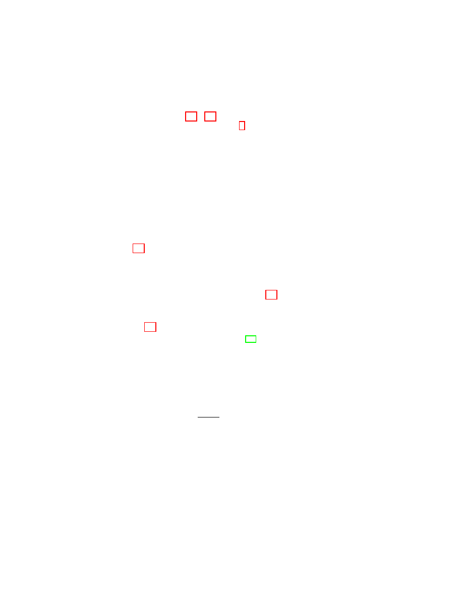
44
1. INTRODUCTION TO PROBLEMS OF MATHEMATICAL PHYSICS
C
∞
0
(Ω) such that f
m
→ f almost everywhere as m → ∞, if |f | ≤ M
almost everywhere.
Proof. By virtue of (9.5)–(9.6), kf − R
(f )k
1
→ 0 as → 0.
Therefore, according to note 6 in Section 8, there exists a subse-
quence {f
m
} of the sequence {R
(f )}
→0
such that f
m
→ f almost
everywhere. The estimate |f
m
| ≤ M is obvious.
9.8.P.
5)
Prove that ku − R
(u)k
C
→ 0 as → 0, if u ∈ C
0
(Ω).
5)
Here and below, kf k
C
= sup
x∈Ω
|f (x)| for f ∈ C( ¯
Ω).
9.9. Definition. L
∞
(Ω) is the space of essentially bounded
functions in Ω, i.e., the space of measurable functions f : Ω → C
such that
kf k
∞
= inf
ω∈Ω
sup
x∈ω
|f (x)| < ∞,
µ(Ω \ ω) = 0.
(9.7)
Condition (9.7) means that the function f is bounded almost every-
where, i.e., ∃M < ∞ such that |f (x)| ≤ M almost everywhere and
kf k
∞
= inf M .
One can readily prove
9.10. Lemma. The space L
∞
(Ω) with the norm (9.7) is a Banach
space,
9.11. Remark. The symbol ∞ in the designation of the space
and the norm (9.7) is justified by the fact that kf k
∞
= lim
p→∞
kf k
p
, if
Ω b R
n
. This fact is proved, for instance, in [71].
9.12. Definition. Let X be a normed space with a norm k · k.
Then X
0
denotes the space of continuous linear functional on X.
The space X
0
is called dual to X.
One can readily prove
9.13. Proposition. The space X
0
equipped with the norm
kf k
0
= sup
x∈X
|hf, xi|
kxk
,
f ∈ X
0
,
is a Banach space. Here, hf, xi is that value of f at x ∈ X.
10. FUNCTIONS OF L
1
loc
AS LINEAR FUNCTIONAL ON C
∞
0
45
9.14. Theorem (F. Riesz, 1910). Let 1 ≤ p < ∞. Then (L
p
)
0
=
L
q
, where 1/p + 1/q = 1 (q = ∞ for p = 1). More exactly:
1) ∀f ∈ L
q
(Ω) ∃F ∈ (L
p
(Ω))
0
, i.e., a linear continuous func-
tional F on L
p
(Ω) such that
hF, ϕi =
Z
Ω
f (x)ϕ(x)dx
∀ϕ ∈ L
p
(Ω);
(9.8)
2) ∀F ∈ (L
p
(Ω))
0
there exists a unique
6)
element (function)
f ∈ L
q
(Ω) such that (9.8) holds;
6)
See note 4 in Section 8
3) the correspondence I : (L
p
)
0
3 F 7−→ f ∈ L
q
is an isomet-
ric isomorphism of Banach spaces, i.e., the mapping I is
linear bijective and kIF k
q
= kF k
0
p
.
Proof. Assertion 1) as well as the estimate kF k
0
p
≤ kf k
q
are
obvious for p = 1. For p > 1 one should use the H¨
older inequality.
Assertion 2) as well as the estimate kF k
0
p
≥ kf k
q
are proven, for
instance, in [71]. Assertion 3) follows from 1) and 2).
9.15. Definition. Let p ∈ [1, ∞]. Then L
p
loc
(Ω) (or simply
L
p
loc
) denotes the space of functions locally integrable in pth power
f : Ω → C, i.e., of the functions such that f · 1
K
∈ L
p
(Ω) ∀K b Ω.
We introduce in L
p
loc
(Ω) the convergence: f
j
→ f in L
p
loc
(Ω) if and
only if k1
K
· (f
j
− f )k
p
→ 0 as j → ∞ ∀K b Ω.
Let us note the obvious fact: if 1 < r < s < ∞, then
P C ( L
∞
loc
( L
s
loc
( L
r
loc
( L
1
loc
.
10. Functions of L
1
loc
as linear functional on C
∞
0
The idea of representability (i.e., of determination) of a function
by its “averagings”, outlined in Sections 1–2 can now be written in
a rather general form as the following
10.1. Theorem. Any function f ∈ L
1
loc
(Ω) can be uniquely
1)
reconstructed by the linear functional
hf, ·i : C
∞
0
(Ω) 3 ϕ 7−→ hf, ϕi =
Z
Ω
f (x)ϕ(x)dx ∈ C
(10.1)

46
1. INTRODUCTION TO PROBLEMS OF MATHEMATICAL PHYSICS
(i.e., by the set of the numbers
n
hf, ϕi
ϕ∈C
∞
0
(Ω)
o
). Moreover, the
correspondence f ←→ hf, ·i, f ∈ L
1
loc
, is an isomorphism.
1)
As an element of the space L
1
loc
(Ω) (see note 4 in Section 8).
Proof. Suppose that two functions f
1
and f
2
correspond to
one functional. Then
R (f
1
− f
2
)ϕ = 0 ∀ϕ ∈ C
∞
0
. This, by virtue of
Lemma 10.2 below, implies that f
1
= f
2
almost everywhere.
10.2. Lemma. Let f ∈ L
1
loc
(Ω). If
R
Ω
f (x)ϕ(x)dx = 0 ∀ϕ ∈
C
∞
0
(Ω), then f = 0 almost everywhere.
Proof. Let ω b Ω. Note that |f | · 1
ω
= f · g, where g(x) =
1
ω
· exp[−i arg f (x)]. (If f is a real function, then g(x) = − sgn f (x) ·
1
ω
(x).) According to Corollary 9.7, there exists a sequence of func-
tions ϕ
n
∈ C
∞
0
(Ω), such that almost everywhere in Ω f · ϕ
n
→ f · g
as n → ∞, and |ϕ
n
| ≤ 1. Since
R
ω
|f | =
R
Ω
f · g and by the Lebesgue
theorem
R
Ω
f · g =
lim
n→∞
R
Ω
f · ϕ
n
, we have
R
ω
|f | = 0, because
R
Ω
f · ϕ
n
= 0. Thus, f = 0 almost everywhere in ω. Hence, by
virtue of arbitrariness of ω b Ω, f = 0 almost everywhere in Ω.
11. Simplest hyperbolic equations. Generalized Sobolev
solutions
In this section we illustrate one of the main achievements of the
theory of distributions on the example of the simplest partial differ-
ential equation u
t
+ u
x
= 0,
1)
which is sometimes called the transfer
equation. It concerns a new meaning of solutions of differential equa-
tions, more exactly, a new (extended) meaning of differential equa-
tions. This meaning allows us to consider correctly some important
problems of mathematical physics which have no solutions in the
usual sense. This new approach to the equations of mathematical
physics and their solutions, designed by S.L. Sobolev in 1935 (see,
for instance, [62]) under the title “generalized solutions”, allows, in
particular, to prove the existence and uniqueness theorem for the
generalized solution of the Cauchy problem:
Lu ≡ u
t
+ u
x
= 0,
(x, t) ∈ R
2
+
= {(x, t) ∈ R
2
| t > 0},
(11.1)
u
t=0
= f (x),
x ∈ R
(11.2)
11. SIMPLEST HYPERBOLIC EQUATIONS
47
for equation (11.1) for any function f ∈ P C(R) (and even f ∈ L
1
loc
;
see Theorem 11.10 below). The theorem is also valid (see P.11.11)
on the continuous dependence of the solution of this problem on
f ∈ L
1
loc
(R).
1)
Here, u
t
and u
x
denote the partial derivatives of the function u(x, t)
with respect to t and x.
Let us clarify the essence of the problem. Equation (11.1) is
equivalent to the system
u
t
+ u
x
· dx/dt = 0,
dx/dt = 1.
Therefore, along the line x = t + a, where a is a real parameter, we
have du(t + a, t)/dt = 0. In other words, u(t + a, t) = u(a, 0) ∀t.
Thus, the function f (x) = lim
t→+0
u(x, t) must necessary be contin-
uous; in this case u(x, t) = f (x − t).
2)
If f is differentiable, then
u(x, t) = f (x − y) is a solution of problem (11.1)–(11.2).
How-
ever, this problem has no solution (differentiable or even contin-
uous), if f is discontinuous, for instance, if f (x) = θ(x), where
θ : R 3 x 7−→ θ(x) ∈ R is the Heaviside function, i.e.,
θ(x) = 1 for x ≥ 0
and
θ(x) = 0 for x < 0.
(11.3)
2)
This formula implies that the graph of the function x 7−→ u(x, t)
for any fixed t can be obtained by the transition (shift) of the graph of the
function f to the right along the axis x on the distance t. It is the reason
why equation (11.1) is sometimes called the transfer equation.
However, consideration of problem (11.1)–(11.2) with the initial
function (11.3) is justified at least by the fact that this problem arises
(as minimum, on the formal level) when studying the propagation of
the plane sonic waves in a certain medium. The appropriate process
is described by the so-called acoustic system of differential equations
u
t
+
1
ρ
p
x
= 0, p
t
+ ρ · c
2
u
x
= 0,
ρ > 0, c > 0.
(11.4)
Here, ρ is the density, c is the characteristic of the compressible
medium, and u = u(x, t) and p = p(x, t) are the velocity and the
pressure at the instant t at the point x. Setting
α = u + p/(ρ · c),
β = u − p/(ρ · c),
48
1. INTRODUCTION TO PROBLEMS OF MATHEMATICAL PHYSICS
we obtain the equivalent system α
t
+ cα
x
= 0, β
t
− cβ
x
= 0 of two
transfer equations. Thus, problem (11.1)–(11.2) with the initial func-
tion (11.3) arises when considering the propagation of sonic waves,
say, for the initial velocity u(x, t) = θ(x) and zero initial pressure.
11.1.P. Show that any solution of the class C
1
of system (11.4)
can be represented in the form
u(x, t) = [ϕ(x − ct) + ψ(x + ct)]/2,
p(x, t) = [ϕ(x − ct) − ψ(x + ct)]/2, where ϕ ∈ C
1
, ψ ∈ C
1
.
(11.5)
11.2.P. Show that the following theorem is valid.
11.3. Theorem. ∀f ∈ C
1
(R) ∀F ∈ C( ¯
R
2
+
) the Cauchy problem
u
t
+ u
x
= F (x, t) in R
2
+
,
u
t=0
= f (x),
x ∈ R
has a unique solution u ∈ C
1
( ¯
R
2
+
).
As has been said, for f (x) = θ(x) problem (11.1)–(11.2) has
no regular solution (i.e., a solution in the usual sense of this word);
nevertheless the arguments which lead to the formula u(x, t) = f (x−
t) as well as this formula suggest to call by the solution of problem
(11.1)–(11.2) the function f (x − t) for whatever function f ∈ P C(R)
(and even f ∈ L
1
loc
(R)), especially, as the following lemma holds.
11.4. Lemma. Let f ∈ L
1
loc
(R) and {f
n
} be a sequence of func-
tions f
n
∈ C
1
(R) such that
3)
f
n
→ f in L
1
loc
(R)
as n → ∞.
Then the function u : R
2
+
3 (x, t) 7−→ u(x, t) = f (x − t) belongs to
L
1
loc
(R
2
+
), and u = lim
n→∞
u
n
in L
1
loc
(R
2
+
), where u(x, t) = f (x − t).
4)
3)
According to Lemma 11.5 below, such a sequence exists.
4)
Note that u
n
(x, t) is a solution of problem (11.1)–(11.2), if u
n
˛
˛
t=0
=
f
n
(x).
Proof. Since f = f
1
+ if
2
and f
k
= f
k
+
− f
k
−
, where f
k
±
=
max(±f
k
, 0), it is sufficient to consider the case f ≥ 0. Let us make

11. SIMPLEST HYPERBOLIC EQUATIONS
49
the change of the variables (x, t) 7−→ (y, t), where y = x − t. Note
that u(x, t) = f (y) and
b
Z
a
d
Z
c
u(x, t)dx
dt ≤
b
Z
a
d−a
Z
c−d
f (y)dy
dt < ∞
for any a, b, c, d such that 0 < a < b, c < d. By virtue of Lemma 8.26,
this implies u ∈ L
1
loc
(R
2
+
). Furthermore, for the same a, b, c, and d
b
Z
a
d
Z
c
|u
n
(x, t) − u(x, t)|dx
dt ≤ (b − a)
d−a
Z
c−b
|f
n
(y) − f (y)|dy → 0
as n −→ ∞.
11.5. Lemma. ∀f ∈ L
1
loc
(R) there exists a sequence of functions
f
n
∈ C
∞
(R) converging to f in L
1
loc
(R).
Proof. Let {ϕ
µ
}
∞
µ=1
be the partition of unity in R (see Sec-
tion 3), ψ
µ
∈ C
∞
0
(R) and ψ
µ
· ϕ
µ
= ϕ
µ
. We have ψ
µ
· f ∈ L
1
(R).
By Theorem 9.5, there exists a sequence {f
µ
n
}
∞
µ=1
of functions f
µ
n
∈
C
∞
(R) such that for any fixed µ: lim
n→∞
kψ
µ
f − f
µ
n
k
1
= 0. Setting
f
n
(x) =
∞
P
µ=1
ϕ
µ
(x)f
µ
n
(x), x ∈ R, we have f
n
∈ C
∞
(R). Note that
∀c > 0 ∃M ∈ N such that
∞
P
µ=1
ϕ
µ
(x) =
M
P
µ=1
ϕ
µ
(x) for |x| < c. Hence,
c
Z
−c
|f (x) − f
n
(x)|dx =
c
Z
−c
f (x) −
M
X
µ=1
ϕ
µ
(x)f
µ
n
(x)
dx
+
c
Z
−c
M
X
µ=1
ϕ
µ
(ψ
µ
f − f
µ
n
)
dx ≤
M
X
µ=1
c
Z
−c
|ψ
µ
f − f
µ
n
|dx.
Therefore,
lim
n→∞
c
Z
−c
|f − f
n
|dx ≤
M
X
µ=1
lim
n→∞
c
Z
−c
|ψ
µ
f − f
µ
n
|dx = 0,
because lim
n→∞
kψ
µ
f − f
µ
n
k
1
= 0.
50
1. INTRODUCTION TO PROBLEMS OF MATHEMATICAL PHYSICS
The definition of the solution of problem (11.1)–(11.2), where
f ∈ L
1
loc
, with the help of the formula u(x, t) = f (x − t) is rather
tempting, however, let us note that it has a serious defect: with
the help of a concrete formula, one can define the solution of only
a small class of problems. Lemma 11.4 suggests a definition free of
this defect.
11.6. Definition. Let f ∈ L
1
loc
(R). We say that u ∈ L
1
loc
(R
2
+
)
is a generalized solution of problem (11.1)–(11.2), if there exists a
sequence of solutions u
n
∈ C
1
( ¯
R
2
+
) of equation (11.1) such that, as
n → ∞,
u
n
→ u in L
1
loc
(R
2
+
)
and
u
n
t→0
→ f in L
1
loc
(R).
Approximative approach to the definition of a generalized so-
lution can be applied to a large class of problems. So, it has been
above constructed (but was not named), for instance, the generalized
solution of the equation ∆E(x) = δ(x) (see (7.9)) as well as the gen-
eralized solution of the problem ∆P = 0 in R
2
+
, P (x, 0) = δ(x) (see
Remark 5.4). However, the approximative definition, in spite of tech-
nical convenience, also has an essential shortage: it does not show
the real mathematical object, the “generalized” differential equation,
whose immediate solution is the defined “generalized solution”.
It is reasonable to search for the appropriate definition of the
generalized solutions of differential equations (and appropriate “gen-
eralized” differential equations), by analyzing the deduction of the
equations of mathematical physics (in the framework of one or an-
other conception of the continuous medium). The analysis fulfilled
in Sections 1–2, Lemma 10.2, and the Ostrogradsky–Gauss formula
(7.2) suggest the suitable definition (as will be seen from Proposi-
tion 11.8).
11.7. Definition. Let f ∈ L
1
loc
(R). A function u ∈ L
1
loc
(R
2
+
) is
called a generalized solution of problem (11.1)–(11.2), if it satisfies
the following equation (so-called integral identity (in ϕ))
Z
R
2
+
(ϕ
t
+ ϕ
x
)u(x, t)dxdt +
Z
R
ϕ(x, 0)f (x)dx = 0
∀ϕ ∈ C
1
0
( ¯
R
2
+
).
(11.6)
11.8. Proposition. If u ∈ C
1
( ¯
R
2
+
), then (11.6) is equivalent to
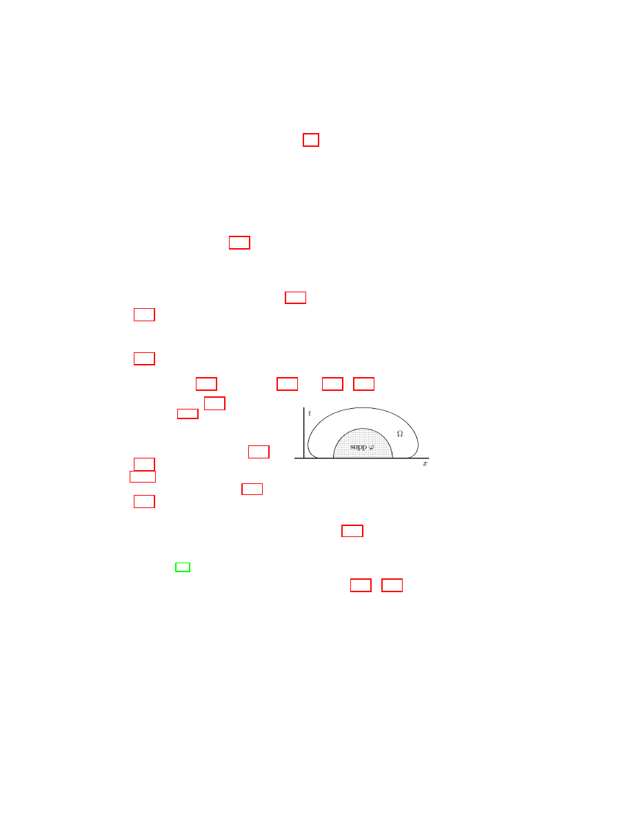
11. SIMPLEST HYPERBOLIC EQUATIONS
51
Proof. Let ϕ ∈ C
1
0
( ¯
R
2
+
) and let Ω be a bounded domain in R
2
+
with the boundary Γ = ∂Ω. Formula (7.2) implies that
Z
Ω
(u
t
+ u
x
)ϕ dx dt +
Z
Ω
(ϕ
t
+ ϕ
x
)u dx dt
=
Z
∂Ω
(ϕ · u)[cos(ν, t) + cos(ν, x)] dΓ.
(11.7)
If supp ϕ ⊂ ¯
Ω and (see Fig.) (supp ϕ ∩ ∂Ω) ⊂ R
x
= {(x, t) ∈ R
2
|
t = 0}, then formula (11.7) can be rewritten in the form
Z
R
2
+
(u
t
+ u
x
)ϕdxdt +
Z
R
2
+
(ϕ
t
+ ϕ
x
)udxdt = −
Z
R
(ϕu)
t=0
dx.
(11.8)
Furthermore, by virtue of Lemma 10.2,
⇐⇒
Z
R
2
+
(u
t
+ u
x
)ϕ dx dt = 0
∀ϕ ∈ C
1
0
( ¯
R
2
+
)
and
(11.2) ⇐⇒
Z
R
f (x)ϕ(x, 0)dx =
Z
R
u
t=0
· ϕ(x, 0)dx ∀ϕ ∈ C
1
0
( ¯
R
2
+
).
This and (11.8) imply that (11.6)⇐⇒(11.1)–(11.2).
Proposition 11.8 shows that
Definition 11.7 is consistent with
the definition of an ordinary (dif-
ferentiable or, as one says, regu-
lar) solution of problem (11.1)–
(11.2). The following Theorem
11.10 justifies the new features
appearing in Definition 11.7 and shows that the integral equality
(11.6) is the same “generalized” differential equation which has been
spoken about.
11.9. Remark. The proof of Proposition 11.8 comes from the
deduction of the Euler–Lagrange equation and the transversality
conditions in calculus of variations proposed by Lagrange (see, for
instance, [56]).
11.10. Theorem. ∀f ∈ L
1
loc
(R) problem (11.1)–(11.2) has a
(unique) generalized solution u ∈ L
1
loc
(R
2
+
).
52
1. INTRODUCTION TO PROBLEMS OF MATHEMATICAL PHYSICS
Proof. First, we prove the existence. Since the function
u : R
2
+
3 (x, t) 7−→ u
n
(x, t) = f (x − t)
is a regular solution of equation (11.1) and satisfies the initial con-
dition u
n
t=0
= f
n
(x), by virtue of proposition 11.8 we have
Z
R
2
+
(ϕ
t
+ ϕ
x
) · u
n
dx dt +
Z
R
f
n
(x)ϕ(x, 0) dx = 0
∀ϕ ∈ C
1
0
( ¯
R
2
+
).
(11.9)
On the other hand, by Lemma 11.4, the sequence {u
n
}
∞
n=1
tends in
L
1
loc
(R
2
+
) to the function u ∈ L
1
loc
(R
2
+
) such that u(x, t) = f (x − t).
It remains to verify that the function u satisfies (11.6). For this
purpose we note: ∀ϕ ∈ C
1
0
( ¯
R
2
+
) ∃a
ϕ
> 0 and b
ϕ
> 0 such that
supp ϕ ⊂ {(x, t) ∈ R
2
| |x| ≤ a
ϕ
, 0 ≤ t ≤ b
ϕ
}.
Therefore,
Z
R
2
+
(u
n
(x, t) − u(x, t))(ϕ
t
+ ϕ
x
)dxdt
≤ [max
(x,t)
|ϕ
t
+ ϕ
x
|] ·
b
ϕ
Z
0
a
ϕ
Z
−a
ϕ
|f
n
(x − t) − f (x − t)|dx
dt
≤ M
ϕ
· b
ϕ
Z
|x|≤a
ϕ
+b
ϕ
|f
n
(x) − f (x)|dx → 0 for n → ∞.
Taking into account (11.9), we obtain (11.6).
Now prove the uniqueness. Let u
1
and u
2
be two generalized
solutions of problem (11.1)–(11.2). Then their difference u = u
1
− u
2
satisfies the relation
R
R
2
+
(ϕ
t
+ ϕ
x
)udxdt = 0 ∀ϕ ∈ C
1
0
( ¯
R
2
+
). Show
that u(x, t) = 0 almost everywhere. By virtue of Lemma 10.2, it is
sufficient to show that the equation
ϕ
t
+ ϕ
x
= g(x, t),
(x, t) ∈ R
2
+
(11.10)
has a solution ϕ ∈ C
1
0
( ¯
R
2
+
) for any g ∈ C
∞
0
(R
2
+
). However, this
follows from P.11.2. Indeed, let T > 0 be such that g(x, t) ≡ 0, if
t ≥ T . We set
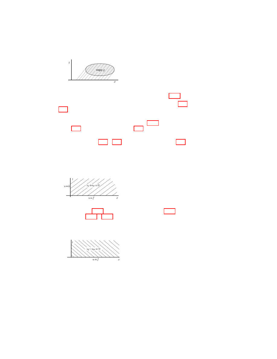
11. SIMPLEST HYPERBOLIC EQUATIONS
53
ϕ(x, t) =
t
Z
T
g(x − t + τ, τ )dτ.
Obviously, (see Fig.) ϕ ∈ C
1
0
( ¯
R
2
+
) and ϕ is a solution of (11.10).
11.11.P. Prove that the generalized solution of problem (11.1)–
(11.2) depends continuously in L
1
loc
(R
2
+
) on the initial function f ∈
L
1
loc
(R).
11.12.P. Analyzing the proof of Theorem 11.10, prove that Def-
inition 11.7 is equivalent to Definition 11.6
11.13.P. Verify directly that the function u(x, t) = θ(x − t) is a
solution of problem (11.1)–(11.2) in the sense of Definition 11.7, if
f (x) = θ(x).
In the exercises below, we assume Q = {(x, t) ∈ R
2
| x > 0,
t > 0}.
11.14.P. Consider the problem
u
t
+ u
x
= 0
in
Q,
(11.11)
u
t=0
= f (x),
x > 0,
(11.12)
u
x=0
= h(t),
t > 0.
(11.13)
This problem is called mixed, because it simultaneously includes the
initial condition (11.12) and the boundary condition (11.13). Show
that problem (11.11)–(11.13) has a (unique) solution u ∈ C
1
( ¯
Q) if
and only if f ∈ C
1
( ¯
R
+
), h ∈ C
1
( ¯
R
+
), ans f (0) = h(0), f
0
(0) =
−h
0
(0).
11.15.P. Show that the following problem
u
t
− u
x
= 0
in Q,
(11.14)
u
t=0
= f (x),
x > 0
(11.15)

54
1. INTRODUCTION TO PROBLEMS OF MATHEMATICAL PHYSICS
has a (unique) solution u ∈ C
1
( ¯
Q) if and only if f ∈ C
1
( ¯
R
+
). Com-
pare with problem (11.11)–(11.13). Compare the characteristics, i.e.,
the families of the straight lines dx/dt = 1 and dx/dt = −1 (shown in
figures), along which the solutions of equations (11.11) and (11.14)
are constant.
11.16.P. Consider a mixed problem for the system of acoustic
equations
u
t
+ (1/ρ)p
x
= 0,
p
t
+ ρc
2
u
x
= 0,
(x, t) ∈ Q,
(11.16)
u
t=0
= f (x),
p
t=0
= g(x),
x > 0,
(11.17)
p
x=0
= h(t),
t > 0,
(11.18)
where f , g, and h are functions from C
1
( ¯
R
+
).
(1) Draw the level lines of the functions u ± (1/ρc)p.
(2) Show that problem (11.16)–(11.18) has a (unique) solution
u ∈ C
1
( ¯
Q), p ∈ C
1
( ¯
Q) if and only if
h(0) = g(0)
and
f
0
(0) + (1/ρc
2
)h
0
(0) = 0.
(11.19)
Show also that this solution (u, p) can be represented by formulae
(11.5), where
ϕ(y) = f (y) + (1/ρc)g(y),
ψ(y) = f (y) − (1/ρc)g(y), if y > 0
(11.20)
and
ϕ(y) = (2/ρc)h(−y/c) + f (−y) − (1/ρc)g(−y), if y ≤ 0. (11.21)
11.17. Remark. Often instead of system (11.4) of the acoustic
equations, the following second order equation is considered
∂
2
p/∂t
2
− c
2
· ∂
2
p/∂x
2
= 0.
This equation obviously follows from system (11.4), if p ∈ C
2
, u ∈
C
2
. This equation is called the string equation, since the graph of
the function p can be interpreted as a form of small oscillations of a
string. The string equation is a special case of the wave equation
p
tt
− c
2
∆p = 0,
p = p(x, t),
x ∈ R
n
, t > 0.
(11.22)
Here, ∆ is the Laplace operator.
For n = 2 the wave equation
describes the oscillations of a membrane, for n = 3 it describes the
oscillations of 3-dimensional medium.
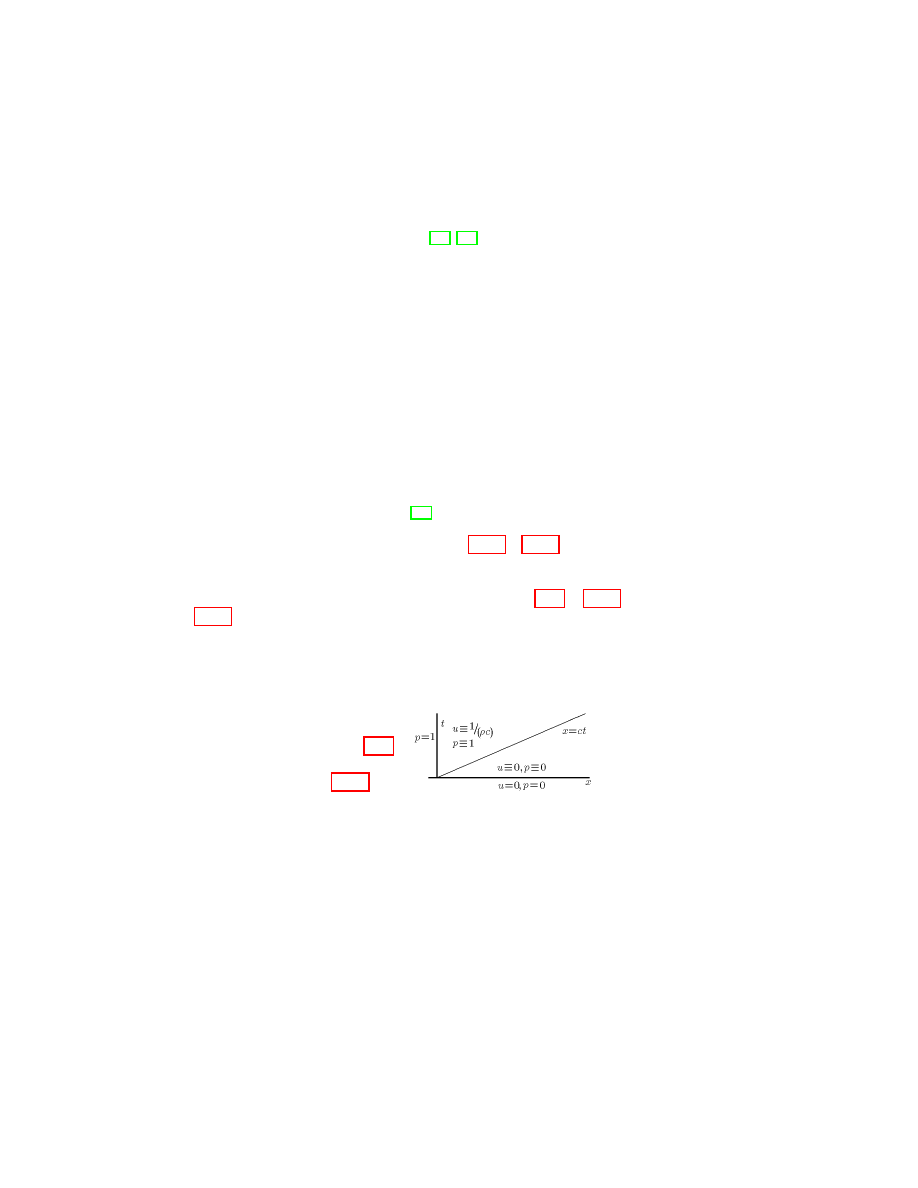
11. SIMPLEST HYPERBOLIC EQUATIONS
55
11.18. Remark. The string equation is remarkable in many as-
pects. It was the first equation in partial derivatives that appeared
in mathematical investigations (B. Teylor, 1713). It was a source of
fruitful discussion (see, for instance, [42, 50]) in which the notion of
a function was developed (d’Alembert, Euler, D. Bernoulli, Fourier,
Riemann,. . . ).
11.19. Remark. Many distinctive properties of some differen-
tial operators A(y, ∂
y
1
, . . . ∂
y
m
), y ∈ Ω are defined by the proper-
ties of the corresponding characteristic polynomials A(y, η
1
, . . . , η
m
)
of the variable η = (η
1
, . . . , η
m
). Thus, the hyperbolic polynomial
τ
2
− ξ
2
(τ
2
− |ξ|
2
) is associated with the string equation u
tt
− u
xx
= 0
(or, more generally, with the wave equation u
tt
− ∆u = 0); the ellip-
tic polynomial |ξ|
2
≡
P
k
ξ
2
k
is associated with the Laplace equation
∆u = 0; the parabolic polynomial τ − |ξ|
2
is associated with the heat
equation u
t
− ∆u = 0. According to the type of the characteristic
polynomial, partial differential equations can be classified into hy-
perbolic equations, elliptic equations, parabolic equation, . . . . (See
exact definitions, for instance, in [48].)
11.20. Example. Consider problem (11.16)–(11.18) with f =
g = 0, h = 1. This means that at the initial instant t = 0 the
velocity u and the pressure p are equal to zero, and on the boundary
x = 0 the pressure p = 1 is maintained. Formulae (11.5), (11.20)–
(11.21) give the following result:
u = 0,
p = 0,
if t < x/c
u = 1/ρc,
p = 1,
if t ≥ x/c
(11.23)
The functions u and p are
discontinuous that is not sur-
prising, because condition (11.9)
does not hold. However, on the
other hand, formulae (11.23) are
in a good accordance with the
physical processes. This yields
11.21.P. Find the appropriate definitions of the generalized so-
lutions for the following problems:
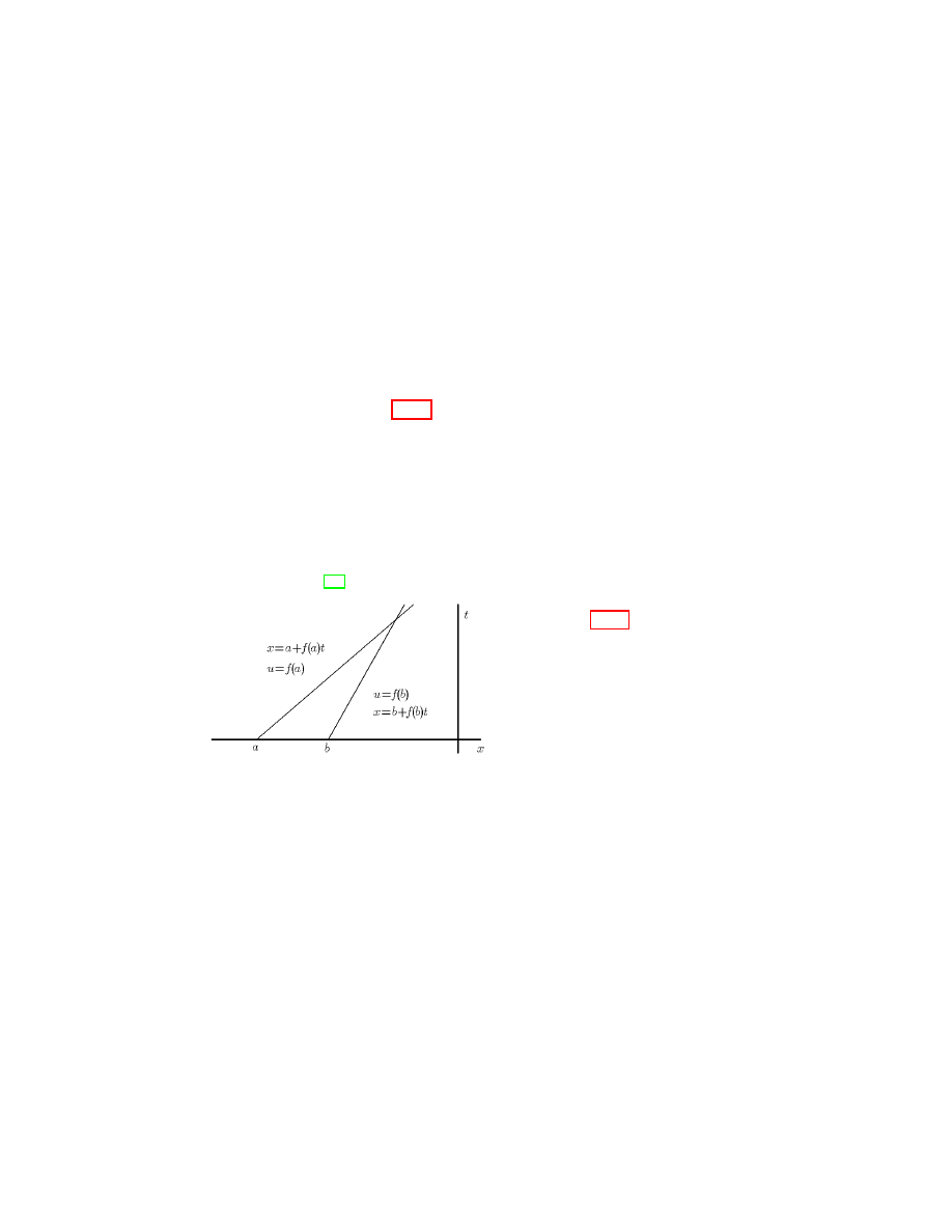
56
1. INTRODUCTION TO PROBLEMS OF MATHEMATICAL PHYSICS
(1) u
t
+ u
x
= F (x, t) in Q = {(x, t) ∈ R
2
| x > 0, t > 0};
u
t=0
= f (x), x > 0; u
x=0
= h(t), t > 0;
(2) u
t
+ (1/ρ)p
x
= F (x, t), p
t
+ ρ · c
2
u
x
= G(x, t) in Q;
u
t=0
= f (x), p
t=0
= g(x), x > 0; u
x=0
= h(t), t > 0.
(3) p
tt
− c
2
p
xx
= F (x, t) in the half-strip Ω = {(x, t) ∈ R
2
+
|
0 < x < 1};
p
t=0
= f (x), p
t
t=0
= g(x), 0 < x < 1;
p
x=0
= h
0
(x),
p
x=1
= h
1
(x), t > 0.
Revise the requirements to the functions f , g, h, F , G, under which
the solutions of these problems belong, say, to the space C
1
, P C
1
or L
1
loc
. Prove the theorems of existence, uniqueness and continuous
dependence (compare with P.11.11).
We conclude this section by consideration of the non-linear equa-
tion
u
t
+ (u
2
/2)
x
= u
xx
+ b
x
(x, t),
u = u(x, t),
(11.24)
where ≥ 0, and b is a given function. This equation is called the
Burgers equation and is considered in hydrodynamics as a model
equation for > 0 of the Navier–Stokes system, and for = 0 of the
Euler system (see [52]).
First, consider
equation (11.24) for
= 0 and b ≡ 0. In
this case, the regu-
lar (of the class C
1
)
solution of this equa-
tion satisfies the sys-
tem dx/dt
=
u,
du/dt = 0.
Thus,
the solution u(x, t)
is constant along the characteristic, i.e., along the curve defined
by the equation dx/dt = u(x, t); hence, this curve is, in fact, the
straight line x = a + f (a)t that depends only on the parameter
a ∈ R and a function f . The function f is determined by the rela-
tions f (a) = dx/dt, dx/dt = u(x, t), i.e., f (x) = u(x, 0). If f is a
decreasing function, for instance, f (x) = − th(x), then the charac-
teristics intersect at some t > 0, and at the point of the intersection
11. SIMPLEST HYPERBOLIC EQUATIONS
57
we have
u(x − 0, t) > u(x + 0, t).
(11.25)
The continuous solution cease to exist. Thus, the Cauchy problem
u
t
+ (u
2
/2)
x
= 0
in R
2
+
,
u
t=0
= f (x),
x ∈ R
(11.26)
has, in general, no continuous solution even for analytic initial data.
This effect is well known in hydrodynamics. It is connected with
arising of the so-called shock waves
5)
which are characterized by a
jump-like change of the density, velocity, etc. Thus, physics suggest
that the solution of problem (11.26) should be sought as a generalized
solution of the class P C
1
.
5)
See Addendum.
Suppose that u is a generalized solution of problem (11.26), and
u has a jump along the curve
γ = {(x, t) ∈ R
2
| x = λ(t), λ ∈ C
1
[α, β]};
more exactly, suppose that (x, t) ∈ γ satisfies condition (11.25).
11.22.P. Prove (compare with P.12.6) that the Hugoni´ot condi-
tion
dλ(t)/dt = [u(λ(t) + 0, t) + u(λ(t) − 0, t)]/2.
(11.27)
holds along this line γ called the break line.
One can show (see, for instance, [52]) that relations (11.25),
(11.27) replace the differential equation u
t
+ (u
2
/2)
x
= 0 on the
break line.
One of the approaches to the study of problem (11.26) is based
on consideration of the Cauchy problem for equation (11.24) for > 0
(and b ≡ 0) with the passage to the limit as → 0 (see, for instance,
[52]). The point is that (for b ≡ 0) equation (11.24) can be reduced,
however surprising it is, to the well studied heat equation. Actually,
the following theorem holds
6)
.
6)
This theorem was proven in 1948 by V.A. Florin and in 1950 was
rediscovered by E. Hopf.
11.23. Theorem. The solution of equation (11.24) can be rep-
resented in the form u = −2(ln G)
x
, where G is the solution of the

58
1. INTRODUCTION TO PROBLEMS OF MATHEMATICAL PHYSICS
linear parabolic equation
G
t
= G
xx
−
b(x, t)
2
G.
(11.28)
Proof. Let u be the solution. Setting
P (x, t) = u(x, t),
Q(x, t) = −u
2
(x, t)/2 + u
x
(x, t) + b(x, t),
we have P
t
= u
t
, Q
x
= −u · u
x
+ u
xx
+ b
x
(x, t). Therefore, P
t
= Q
x
.
Thus, the function is defined
F (x, t) =
(x,t)
Z
(0,0)
P dx + Qdt.
We have F
x
= P , F
t
= Q. Hence, F
t
+ (F
x
)
2
/2 − F
xx
= b. Introduc-
ing the function G = exp[−F/2], we obtain that G is the solution
of equation (11.28) and u = −2(ln G)
x
, because u = F
x
.
CHAPTER 2
The spaces D
[
, D
#
and D
0
. Elements of
the distribution theory (generalized
function in the sense of L. Schwartz)
12. The space D
[
of the Sobolev derivatives
The definition of the generalized solution u ∈ L
1
loc
to one or an-
other problem of mathematical physics given by Sobolev [61] and,
in particular, Definition 11.7 is based on Theorem 10.1 and the
Ostrogradsky–Gauss formula (7.2). Let us recall that Theorem 10.1
asserts the equivalence of the two following representations of an
element u ∈ L
1
loc
:
1) Ω 3 x 7−→ u(x)
and
2) C
∞
0
(Ω) 3 ϕ 7−→
Z
Ω
u(x)ϕ(x)dx,
and formula (7.2) implies that, for the differential operator ∂
α
=
∂
|α|
/∂x
α
1
1
. . . ∂x
α
n
n
and any function u ∈ C
|α|
(Ω) the following iden-
tity is valid:
Z
Ω
(∂
α
u(x))ϕ(x)dx = (−1)
|α|
Z
Ω
u(x)∂
α
ϕ(x)dx
∀ϕ ∈ C
∞
0
(Ω).
Thus, the functional
∂
α
u : C
∞
0
(Ω) 3 ϕ 7−→ h∂
α
u, ϕi = (−1)
|α|
Z
Ω
u(x)∂
α
ϕ(x)dx
∀ϕ ∈ C
∞
0
(Ω)
(12.1)
determines the function ∂
α
u(x), if u ∈ C
|α|
(Ω). Since functional
(12.1) is also defined for u ∈ L
1
loc
(Ω), one can, tracing S.L. Sobolev’s
approach, give the following definition.
59

60
2. THE SPACES D
[
, D
#
AND D
0
12.1. Definition. Let α = (α
1
, . . . , α
n
) be a multiindex. The
weak derivative of order α of the function u ∈ L
1
loc
(Ω) is defined as
the functional ∂
α
u given by formula (12.1).
Using Theorem 10.1, formula (7.2), and the identity
Z
Ω
a(x)(∂
α
u(x))ϕ(x) dx = (−1)
|α|
Z
Ω
u(x)∂
α
(a(x)ϕ(x)) dx,
u ∈ C
|α|
(Ω),
ϕ ∈ C
∞
0
(Ω),
which is valid for any function a ∈ C
∞
(Ω), we introduce the opera-
tion of multiplication of the functional ∂
α
u, where u ∈ L
1
loc
(Ω), by
a function a ∈ C
∞
(Ω) with the help of the formula
a∂
α
u : C
∞
0
(Ω) 3 ϕ 7−→ (−1)
|α|
Z
Ω
u(x)∂
α
(a(x)ϕ(x))dx ∈ C. (12.2)
12.2. Definition. The space of Sobolev derivatives is the space
of functionals of the form
P
|α|<∞
∂
α
u
α
, where α is a multiindex and
u ∈ L
1
loc
(Ω), equipped with the operation of multiplication by for-
mula (12.2). This space is denoted by D
[
(Ω).
12.3. Example. Let the function x
+
∈ L
1
loc
(R) be defined in
the following way: x
+
= x for x > 0, x
+
= 0 for x < 0. Let us find
its derivatives. We have
hx
0
+
, ϕi = −hx
+
, ϕ
0
i = −
Z
R
x
+
ϕ
0
(x)dx = −
Z
R
+
xϕ
0
(x)dx
= −xϕ(x)
∞
0
+
∞
Z
0
ϕ(x)dx =
Z
R
θ(x)ϕ(x)dx = hθ, ϕi,
i.e., x
0
+
= Θ is the Heaviside function. Now find x
00
+
, i.e., Θ
0
. We
have
hΘ
0
, ϕi = −hΘ, ϕ
0
i = −
∞
Z
0
ϕ
0
(x)dx = −ϕ(x)
∞
0
= ϕ(0) = hδ, ϕi,
(12.3)

12. THE SPACE D
[
OF THE SOBOLEV DERIVATIVES
61
i.e., Θ
0
= δ(x) is the Dirac δ-function. In the same way one can find
any derivative of the δ-function of order k. We have
hδ
(k)
, ϕi = −hδ
(k−1)
, ϕ
0
i = · · · = (−1)
k
hδ, ϕ
(k)
i = (−1)
k
ϕ
(k)
(0).
(12.4)
12.4.P. Let Θ
∈ C
∞
(R), 0 ≤ Θ
(x) ≤ 1, and Θ
(x) ≡ 1 for
x > and Θ
(x) ≡ 0 for x < −. Let us set δ
(x) = Θ
0
(x). Show
that lim
→0
hδ
(k)
, ϕi = (−1)
k
ϕ
(k)
(0) ∀k ≥ 0, ∀ϕ ∈ C
∞
0
(R).
12.5. Remark. Formulae (12.4) allow us to extend the func-
tional δ
(k)
from the functional space C
∞
0
(R) to the space of func-
tions k-times continuously differentiable at the point x = 0 (see
Definition 2.2). On the other hand, formula (12.3) is not defined on
the space C(R), because the functional Θ is not defined on C(R).
Define the function Θ
±
: R
n
3 x 7→ Θ
±
(x) by the following
formula
Θ
±
(x) = 1
Q
±
(x), x ∈ R,
Q
±
= {x = (x
1
, . . . , x
n
) ∈ R
n
| ±x
k
> 0 ∀k}.
(12.5)
If n = 1, then Θ
+
= Θ is the Heaviside function, and Θ
−
= 1 − Θ
+
(in L
1
loc
).
12.6. P. (cf. P.11.22). Let F ∈ C
1
(R), λ ∈ C
1
(R), u
±
∈
C
1
(R
2
). Let, for (x, t) ∈ Ω ⊂ R
2
, u(x, t) = u
+
(x, t)Θ
+
(x − λ(t)) +
u
−
(x, t)Θ
−
(x − λ(t)). Find u
t
and (F (u))
x
, noting that F (u(x, t)) =
F (u
+
(x, t))Θ
+
(x − λ(t)) + F (u
−
(x, t))Θ
−
(x − λ(t)). Show that u
t
+
(F (u))
x
= 0 almost everywhere in Ω if and only if, first, u
t
+
(F (u))
x
≡ 0 in Ω \ γ, where γ = {(x, t) ∈ R
2
| x = λ(t)}, and
second, the Hugoni´
ot condition
dλ(t)
dt
=
F (u(x+0,t)−F (u(x−0,t)
u(x+0,t)−u(x−0,t)
holds
on the line γ.
12.7.P. Check (see (12.5)) that
∂
n
∂x
1
...∂x
n
Θ
+
= δ(x), x ∈ R
n
.
12.8. P. Show that the function E(x, t) = Θ(t − |x|)/2 is the
fundamental solution of the string operator, i.e.,
(∂
2
/∂t
2
− ∂
2
/∂x
2
)E(x, t) = δ(x, t).
Here, δ(x, t) is that δ-function in R × R, i.e., hδ(x, t), ϕi = ϕ(0, 0)
∀ϕ ∈ C
∞
0
(R × R).

62
2. THE SPACES D
[
, D
#
AND D
0
12.9.P. Noting that, for ϕ ∈ C
∞
0
(R),
lim
→0
Z
|x|>
ln |x| · ϕ
0
(x)dx = lim
→0
ln (ϕ(−) − ϕ()) −
Z
|x|>
ϕ(x)
x
dx
,
prove that
d
dx
ln |x| = v.p.
1
x
, i.e.,
d
dx
ln |x|, ϕ
= v.p.
R
∞
−∞
ϕ(x)
x
dx
∀ϕ ∈ C
∞
0
(R), where v.p.
R
∞
−∞
x
−1
ϕ(x) dx is so-called the principal
value = valeur principal (French) of the integral
R
∞
−∞
x
−1
ϕ(x)dx
defined by the formula
v.p.
∞
Z
−∞
x
−1
ϕ(x)dx = lim
→0
Z
|x|>
x
−1
ϕ(x)dx.
(12.6)
12.10. P. Taking into account that ln(x ± i) = ln |x ± i| +
i arg(x ± i) → ln |x| ± iπΘ(−x) as → +0, prove the simplest ver-
sion the Sokhotsky formulae (very widespread in the mathematical
physics (see, for instance, [38]))
1
x ∓ i0
= v.p.
1
x
± iπδ(x),
(12.7)
i.e., prove that lim
→+0
R
∞
−∞
ϕ(x)dx
x∓i
= v.p.
R
∞
−∞
ϕ(x)
x
dx ± iπϕ(0) ∀ϕ ∈
C
∞
0
(R).
12.11. Remark. Formulae (12.7) imply that
δ(x) = f (x − i0) − f (x + i0),
where
f (x + iy) =
1
2πi
(x + iy)
−1
,
(12.8)
i.e., the δ-function being an element of D
[
(R) admits the represen-
tation in the form of the difference of boundary values on the real
axis of two functions analytic in C
+
and in C
−
, respectively, where
C
±
= {z = x + iy ∈ C | ±y > 0}. This simple observation has deep
generalizations in the theory of hyperfunctions (see, for instance,
[43, 53]).
12.12. Remark. Any continuous function F ∈ C(R) has, as
an element of the space L
1
loc
, the Sobolev derivative F
0
∈ D
[
(R).
If this derivative is a locally integrable function, in other words, if
13. THE SPACE D
#
OF GENERALIZED FUNCTIONS
63
F (x) =
R
x
a
f (y) dy + F (a), where f ∈ L
1
loc
(R), then Theorem 8.27
implies that
F
0
(x) = lim
σ→0
σ
−1
(F (x + σ) − F (x)) for almost all x ∈ R. (12.9)
In this case, formula (12.9) totally determines the Sobolev derivative
F
0
. Emphasize that the last assertion does not hold (even under the
assumption that formula (12.9) is valid), if F
0
/
∈ L
1
loc
(R). Thus, for
instance, the Cantor ladder (see [36] or [56]) corresponding to the
Cantor set of zero measure (see hint to P.8.23), i.e., a continuous
monotone function K ∈ C[0, 1] with the value (2k − 1) · 2
−n
in kth
(k = 1, . . . , 2
n−1
) interval I
n
=]a
k
n
, b
k
n
[ of rank n (see hint to P.8.23)
has, for almost all x ∈ [0, 1], zero derivative but its Sobolev derivative
K
0
is non-zero. Namely,
K
0
=
∞
X
n=1
2
n−1
X
k=1
(2k − 1) · 2
−n
(δ(x − b
k
n
) − δ(x − a
k
n
)).
(12.10)
12.13.P. Prove formula (12.10).
13. The space D
#
of generalized functions
The elements of the space D
[
were defined as finite linear com-
binations of the functionals ∂
α
u
α
(12.1), i.e., of the derivatives of
the functions u
α
∈ L
1
loc
.
If we neglect the concrete form of the
functionals, i.e., consider an arbitrary linear functional
f : C
∞
0
(Ω) 3 ϕ 7−→ hf, ϕi ∈ C,
(13.1)
then we obtain an element of the space D
#
(Ω), which will be called
a generalized function (in the domain Ω). Let us give the exact
13.1. Definition. D
#
(Ω) is the space of all linear functionals
(13.1) in which the operations of differentiation ∂
α
and multipli-
cation by a function a ∈ C
∞
(Ω) are introduced by the following
formulae:
h∂
α
f, ϕi = (−1)
|α|
hf, ∂
α
ϕi,
haf, ϕi = hf, aϕi ∀ϕ ∈ C
∞
0
(Ω).
(13.2)
13.2. Example. f =
∞
P
k=0
δ
(k)
(x − k), x ∈ R, i.e., hf, ϕi =
∞
P
k=0
(−1)
k
ϕ
(k)
(k) ∀ϕ ∈ C
∞
0
(R). Obviously, f ∈ D
#
(R), and f /
∈

64
2. THE SPACES D
[
, D
#
AND D
0
D
[
(R). Thus, D
[
(Ω) ( D
#
(Ω). By the way, the following lemma is
valid.
13.3. Lemma (P. du Bois Reimond). If f ∈ D
#
(R) and f
0
= 0,
then f = const. (Thus, f ∈ D
[
(R).)
Proof. We have hf
0
, ϕi = hf, ϕ
0
i = 0 ∀ϕ ∈ C
∞
0
(R). Let us
take a function ϕ
0
∈ C
∞
0
(R) such that
R ϕ
0
= 1. Any function
ϕ ∈ C
∞
0
(R) can be represented in the form ϕ = ϕ
1
+
R ϕ
ϕ
0
, where
ϕ
1
= ϕ−
R ϕ
ϕ
0
. Note that
R ϕ
1
= 0. Setting ψ(x) =
R
x
−∞
ϕ
1
(ξ)dξ,
we have ψ ∈ C
∞
0
(R) and ψ
0
= ϕ
1
. Therefore, hf, ϕi = hf, ψ
0
i +
hf,
R ϕ
ϕ
0
i. Since hf, ψ
0
i = 0, it follows that hf, ϕi = C
R ϕ, where
C = hf, ϕ
0
i.
Generalizing the notion of a δ-sequence, we introduce
13.4. Definition. A sequence of functionals f
ν
∈ D
#
is said
weakly converges to f ∈ D
#
on the space Φ ⊃ C
∞
0
, if f
ν
−→ f in
D
#
on the space Φ, i.e., lim
ν→∞
hf
ν
, ϕi = hf, ϕi ∀ϕ ∈ Φ. If Φ = C
∞
0
,
then the words “on the space C
∞
0
” are usually omitted.
13.5. Definition. We say that a subspace X of the space D
#
is
complete with respect to the weak convergence, if, for any sequence
{f
ν
}
∞
ν=1
of functionals f
ν
∈ X satisfying the condition
hf
ν
− f
µ
, ϕi −→ 0
∀ϕ ∈ C
∞
0
as ν, µ −→ ∞,
there exists f ∈ X such that f
ν
→ f in D
#
.
13.6.P. Show that D
[
is not complete with respect to the weak
convergence.
13.7.P. Show that D
#
is complete with respect to the weak con-
vergence.
13.8. Lemma. If f
ν
→ f in D
#
on the space Φ ⊃ C
∞
0
, then
∂
α
f
ν
→ ∂
α
f in D
#
on the space Φ for any α.
Proof. h∂
α
f
ν
, ϕi = (−1)
|α|
hf
ν
, ∂
α
ϕi −→ (−1)
|α|
hf, ∂
α
ϕi =
h∂
α
f, ϕi.
13.9. Example. Let f
ν
=
sin νx
ν
, i.e., hf
ν
, ϕi =
R
R
sin νx
ν
ϕ(x)dx.
Then f
0
ν
= cos νx, f
00
ν
= −ν · sin νx, . . . We have hf
ν
, ϕi −→ 0
∀ϕ ∈ C
∞
0
as ν → ∞. Thus, cos νx → 0 in D
#
, ν sin νx → 0 in
D
#
, . . .
13. THE SPACE D
#
OF GENERALIZED FUNCTIONS
65
13.10. Lemma. Let a = (a
1
, . . . , a
n
) ∈ Ω ⊂ R
n
. Suppose that
a sequence {f
ν
}
∞
ν=1
of functions f
ν
∈ L
1
loc
(Ω) and a point b =
(b
1
, . . . , b
n
)
1)
∈ Π, where
Π = {x = (x
1
, . . . , x
n
) ∈ R
n
| |x
k
− a
k
| < σ
k
, σ
k
> 0 ∀k} ⊂ Ω,
are such that, for F
ν
(x) =
R
x
1
b
1
. . .
R
x
n
b
n
f
ν
(y)dy
1
. . . dy
n
, the following
two properties hold:
1)
As b = (b
1
, . . . , b
n
) one can take any point of Π such that b
k
< a
k
∀k.
(1) |F
ν
(x)| ≤ G(x), x ∈ Ω, where G ∈ L
1
loc
(Ω),
(2) F
ν
(x) → Θ
+
(x − a) almost everywhere in Ω, where Θ
+
is
defined in (12.5).
Then f
ν
weakly converges to δ(x − a) on the space
Φ = {ϕ ∈ C(Ω) | ϕ ∈ L
1
(Ω), ∂
n
ϕ/∂x
1
. . . ∂x
n
∈ L
1
(Ω)}.
(13.3)
Proof. Using Theorems 8.20, 8.24, and 8.27, we obtain, for any
ϕ ∈ Φ,
hf
ν
, ϕi =
∂
n
F
ν
∂x
1
. . . ∂x
n
, ϕ
= (−1)
n
F
ν
,
∂
n
ϕ
∂x
1
. . . ∂x
n
= (−1)
n
Z
Ω
F
ν
(x)
∂
n
ϕ(x)
∂x
1
. . . ∂x
n
dx −→ (−1)
n
∞
Z
a
1
. . .
∞
Z
a
n
∂
n
ϕ(x)dx
∂x
1
. . . ∂x
n
= −(−1)
n
∞
Z
a
2
. . .
∞
Z
a
n
∂
n−1
ϕ(x)dx
∂x
2
. . . ∂x
n
dx
2
. . . dx
n
= ϕ(a).
13.11.P. Using Lemma 13.10, solve problems P.4.3 and P.4.4.
Let us generalize the notion of the support of a function (see
Section 3), assuming, in particular, an exact meaning to the phrase
usual for physicists: “δ(x) = 0 for x 6= 0”.
13.12. Definition. Let f ∈ D
#
(Ω), and ω be an open set in
Ω. We say that f is zero (vanishes) on ω (and write f
ω
= 0 or
f (x) = 0 for x ∈ Ω), if hf, ϕi = 0 ∀ϕ ∈ C
∞
0
(ω).

66
2. THE SPACES D
[
, D
#
AND D
0
13.13. Definition. The annihilating set of a functional f ∈
D
#
(Ω) is the maximal open set Ω
0
= Ω
0
(f ) ⊂ Ω on which f is zero,
i.e., f
Ω
0
= 0, and the condition f
ω
= 0 implies ω ⊂ Ω
0
.
It is clear that Ω
0
(f ) is the union of ω ⊂ Ω such that f
ω
= 0.
13.14. Definition. Let f ∈ D
#
(Ω). The support of the func-
tional f , denoted by supp f , is the completion to the annihilating set
Ω
0
(f ), i.e., the set Ω \ Ω
0
(f ).
13.15.P. Let f ∈ D
#
(Ω). Check that x ∈ supp f if and only if,
for any neighbourhood ω ⊂ Ω of the point x there exists a function
ϕ ∈ C
∞
0
(ω) such that hf, ϕi 6= 0. Verify also that Definition 13.14
is equivalent to Definition 3.1.4, if f ∈ C(Ω).
13.16.P. Find supp δ
(α)
(x) and supp[(x
1
+ · · · + x
n
)δ
(α)
(x)].
13.17.P. Let f ∈ D
#
(Ω), a ∈ C
∞
, and a(x) = 1 for x ∈ supp f .
Is it true that a · f = f ?
13.18.P. Let ω be an open set in Ω such that ω ⊃ supp f , f ∈
D
#
(Ω). Show that af = f , if a(x) = 1 for x ∈ ω.
13.19.P. Let f ∈ D
#
(Ω) be a generalized function with a com-
pact support. Show that the formula hF, ϕi = hf, ψϕi ∀ϕ ∈ C
∞
(Ω),
ψ ∈ C
∞
0
(Ω), where ψ ≡ 1 on an open set ω ⊃ supp f defines the ex-
tension of the functional f onto the space C
∞
(Ω), i.e., F is a linear
functional on C
∞
(Ω) such that hF, ϕi = hf, ϕi ∀ϕ ∈ C
∞
0
(Ω).
14. The problem of regularization
The idea of representability of a function f : Ω −→ C with
the help of its “averaging” functional (10.1) concerned only locally
integrable functions. However, in many problems of analysis, an
important role is played by functions which are not locally integrable.
This is the reason of arising of the so-called problem of regularization:
let g : Ω 3 x 7→ g(x) be a function locally integrable everywhere in
Ω except a subset N ⊂ Ω. It is required to find functionals f ∈ D
#
such that
hf, ϕi =
Z
Ω
g(x)ϕ(x) dx
∀ϕ ∈ C
∞
0
(Ω \ N ).
(14.1)

14. THE PROBLEM OF REGULARIZATION
67
In this case one says that the functional f regularizes the (di-
vergent) integral
R
Ω
g(x) dx.
It is clear that the functionals f satisfying (14.1) can be repre-
sented in the form
f = f
0
+ f
1
,
f
0
∈ F
0
,
where f
1
is a particular solution of the problem of regularization (i.e.,
f
1
satisfies (14.1)), and F
0
is the linear subspace of the functionals
f
0
∈ D
#
(Ω) such that
hf
0
, ϕi = 0
∀ϕ ∈ C
∞
0
(Ω \ N ).
(14.2)
The question of description of the subspace F
0
is connected only
with the set N ⊃ supp f
0
. In the case when N = x
0
∈ Ω, this
question, i.e., the problem concerning the general form of function-
als with a point support, is considered in Section 15. As for the
particular solution of the problem regularization, we conclude this
section by consideration of the regularization for 1/P , where P is a
polynomial in the variable x ∈ R.
14.1. Example. Consider the regularization of the function 1/x.
In other words, find the functional f ∈ D
#
(R) which satisfies the
condition: x · f = 1. Note (see (12.6)) that
v.p.
1
x
, ϕ
=
∞
Z
−∞
1
x
ϕ(x) dx
∀ϕ ∈ C
∞
0
(R \ 0).
Thus, the functional v.p.(1/x) regularizes the function 1/x. Since
hδ, ϕi = 0 ∀ϕ ∈ C
∞
0
(R \ 0), it follows that v.p.(1/x) + C · δ(x), where
C ∈ C; therefore, (see (12.7)) functional 1/(x ± i0) also regularize
the function 1/x.
14.2.P. Check that
v.p.
1
x
, ϕ
=
∞
Z
−∞
ϕ(x) − ϕ(−x)
2x
dx
∀ϕ ∈ C
∞
0
(R).

68
2. THE SPACES D
[
, D
#
AND D
0
14.3. P. Let m ≥ 1, and a ∈ C
∞
0
(R). Define, for k ≥ 2, the
functional v.p.(1/x
k
) ∈ D
#
(R) by the formulae:
v.p.
1
x
k
, ϕ
=
∞
Z
0
1
x
k
ϕ(x) + ϕ(−x) − 2
ϕ(0) + · · · +
x
k−2
(k − 2)!
ϕ
(k−2)
(0)
dx
for k = 2m and
v.p.
1
x
k
, ϕ
=
∞
Z
0
1
x
k
ϕ(x)
+ ϕ(−x) − 2
xϕ
0
(0) + · · · +
x
k−2
(k − 2)!
ϕ
(k−2)
(0)
dx
for k = 2m + 1.
Show that the functional v.p.(1/x
k
) regularizes the function 1/x
k
.
14.4.P. (Compare with P.16.25). Find the solution f ∈ D
#
(R)
of the equation P (x)f = 1. In other words, regularize the integral
R
∞
−∞
P
−1
(x)ϕ(x)dx, where P is a polynomial.
15. Generalized functions with a point support. The Borel
theorem
It has been shown in Section 14 that the mean value problem for
a function locally integrable everywhere in Ω ⊂ R
n
except a point
ξ ∈ Ω leads to the question on the general form of the functional
f ∈ D
#
(Ω) concentrated at the point ξ, i.e., satisfying the condition:
supp f = ξ. It is clear (see P.13.16), that a finite sum of the δ-
function and its derivatives concentrated at the point ξ, i.e., the
sum
X
|α|≤N
c
α
δ
(α)
(x − ξ),
c
α
∈ C, N ∈ N
(15.1)
is an example of such a functional.
However, is the sum (15.1) the general form of a functional f ∈
D
#
, whose support is concentrated at the point ξ? One can show
that the answer to this question is negative, however, the following
theorem holds.

15. GENERALIZED FUNCTIONS WITH A POINT SUPPORT
69
15.1. Theorem. If f ∈ D
#
and f =
P
α
c
α
δ
(α)
(x − ξ), then
c
α
= 0 for |α| > N
f
for some N
f
.
Proof. According to the Borel theorem below, there exists a
function ϕ ∈ C
∞
0
(Ω) such that, for any α
∂
α
ϕ(x)
x=ξ
= (−1)
|α|
/c
α
,
if c
α
6= 0
and
∂
α
ϕ(x)
x=ξ
= 0,
if c
α
= 0.
For such a function ϕ, we have
P
α
c
α
δ
(α)
(x − ξ), ϕ
=
P
α
1, where
the sum is taken over α for which c
α
6= 0.
15.2. Theorem (E. Borel). For any set of numbers a
α
∈ C,
parametrized by the multiindices α = (α
1
, . . . , α
n
), and for any point
ξ ∈ Ω ⊂ R
n
, there exists a function ϕ ∈ C
∞
0
(Ω) such that ∂
α
ϕ
x=ξ
=
a
α
∀α.
Proof. Without loss of generality, we can assume that ξ = 0 ∈
Ω. If the coefficients a
α
grow not very fast as |α| → ∞, more exactly,
if there exist M > 0 and ρ > 0 such that
P
|α|=k
a
α
≤ M ρ
−k
∀k ∈ N,
then the existence of the function required is obvious. Actually, since
in the case considered the series
P
α
a
α
x
α
/α!, where α! = α
1
!·· · ··α
n
!,
converges in the ball B
ρ
= {x ∈ R
n
| |x| < ρ}, we can take as the
required function the following one
ϕ(x) = ψ(x/ρ)
X
α
a
α
x
α
/α! ∈ C
∞
0
(B
ρ
) ⊂ C
∞
0
(Ω),
where
ψ ∈ C
∞
0
(R
n
),
ψ = 0 for |x| > 1, ψ = 1 for |x| < 1/2.
However, in the general case, the series
P
α
a
α
x
α
/α! can diverge
in B
ρ
. What is the reason of the divergence? Obviously, because it
is impossible to guarantee the sufficiently fast decrease of a
α
x
α
/α!
as |α| → ∞ for all x belonging to a fixed ball B
ρ
. One can try to
improve the situation, by considering the series
X
α
ψ(x/ρ
α
) · a
α
x
α
/α!,
(15.2)

70
2. THE SPACES D
[
, D
#
AND D
0
where ρ
α
converges sufficiently fast to zero as |α| → ∞. If it occurs
that series (15.2) converges to a function ϕ ∈ C
∞
, then, as one
can easily see, ϕ ∈ C
∞
0
(Ω) and ∂
α
ϕ
x=0
= a
α
.
Indeed, setting
γ = (γ
1
, . . . , γ
n
) ≤ β = (β
1
, . . . , β
n
) by definition, if γ
k
≤ β
k
∀k, and
β − γ = (β
1
− γ
1
, . . . , β
n
− γ
n
), we have
∂
α
ϕ
x=0
=
X
β
(a
β
/β!)
X
γ≤α
α!
γ!(α − γ)!
∂
a−γ
ψ
x=0
∂
γ
x
β
x=0
=
X
β
(a
β
/β!) ∂
α
x
β
x=0
=
X
β6=α
(a
β
/β!) ∂
α
x
β
x=0
+ a
α
= a
α
.
It remains to show that series (15.2) converges to ϕ ∈ C
∞
(Ω). Note
that since
P
α
=
P
|α|≤k
+
P
|α|>k
, it is sufficient to verify that there exist
numbers ρ
α
< 1 such that
X
j>k
X
|α|=j
ψ(x/ρ
α
)a
α
x
α
/α! ∈ C
k
(Ω)
∀k.
Let us try to find ρ
α
= ρ
j
depending only on j = |α|. If we can
establish that ∀β such that |β| ≤ k, the following inequality holds
∂
β
(ψ(x/ρ
|α|
)a
α
x
α
/α!
≤ C
α
ρ
α
,
(15.3)
where C
α
= C
α
(ψ) < ∞, then, taking ρ
j
= 2
−j
P
|α|=j
C
α
!
−1
, we
obtain
X
j>k
X
|α|=j
∂
β
(ψ(x/ρ
|α|
)a
α
x
α
/α!
≤
X
j>k
ρ
j
X
|α|=j
C
α
≤ 1.
15. GENERALIZED FUNCTIONS WITH A POINT SUPPORT
71
Thus, it remains to prove (15.3). For |α| > k ≥ |β|, we have
∂
β
x
(ψ
x
ρ
|α|
a
α
x
α
α!
)
≤
|a
α
|
α!
X
γ≤β
β!
γ!(β − γ)!
∂
γ
x
ψ
x
ρ
|α|
· |∂
β−γ
x
α
|
≤
|a
α
|x
α
α!
X
γ≤β
β!
γ!(β − α)!
1
ρ
|α|
|γ|
×
∂
γ
t
ψ(t)
t=x/ρ
|α|
· x
α−β+γ
· α
≤|a
α
|
X
γ≤β
β!
γ!(β − α)!
·
∂
γ
t
ψ(t)
t=x/ρ
|α|
· ρ
|α|
.
Now return to the question on the general form of the generalized
function f ∈ D
#
(Ω) with the support at the point ξ = 0 ∈ Ω. First
of all, note (see P.13.19) that, for any function a ∈ C
∞
0
(Ω) such
that a ≡ 1 in a neighbourhood of the point ξ = 0, the formula
hf, ϕi = hf, aϕi ∀ϕ ∈ C
∞
(Ω) is valid. In particular, the functional
f is defined on the polynomials. Setting c
α
= (−1)
|α|
hf, x
α
/α!i, we
obtain
hf, ϕi =
X
|α|<N
c
α
hδ
(α)
, ϕi + hf, r
N
i
∀N,
where
r
N
(x) = a
x
N
ϕ(x) −
X
|α|<N
ϕ
(α)
(0)x
α
/α!
,
0 <
N
< 1.
(15.4)
It is rather tempting to assume that, for an appropriate sequence
{
N
}
∞
N =1
, 0 <
N
< 1, the following condition holds:
hf, r
N
i −→ 0
as
N −→ ∞,
(15.5)
because in this case Theorem 15.1 implies the obvious
15.3. Proposition. If f ∈ D
#
(Ω), supp f = 0 ∈ Ω and (15.5)
is valid, then ∃N ∈ N such that f =
P
|α|≤N
c
α
δ
(α)
.
However, in general, condition (15.5) does not hold, if f ∈ D
#
.
An appropriate example can be constructed with the help of so-called
Hamel basis (see, for instance, [36]).
72
2. THE SPACES D
[
, D
#
AND D
0
16. The space D
0
of generalized functions (distributions by
L. Schwartz)
The wish seems natural to have a theory of generalized functions
in which condition (15.5) is satisfied, hence, Proposition 15.3 holds.
This modest wish (leading, as one can see below, to the theory of
the Schwartz distributions) suggests the following:
1) introduce a convergence in the space C
∞
0
(Ω) such that for
this convergence
lim
N →∞
r
N
= 0 ∈ C
∞
0
(Ω),
(16.1)
where r
N
is defined in (15.4) for some suitable
N
∈]0, 1[;
2) consider below only the functionals f ∈ D
#
(Ω), which are
continuous with respect to the convergence introduced.
It is clear that one can introduce different convergences accord-
ing to which r
N
→ 0 as N → ∞. Which one should be chosen?
Considering this question, one should take into account that the
choice of one or another convergence also determines the subspace
of linear functionals on C
∞
0
that are continuous with respect to this
convergence. Therefore, it seems advisable to add to items 1) and
2) above the following requirement:
3) the space of functionals continuous with respect to the
convergence introduced must include the space D
[
of the
Sobolev derivatives (since this space, as has been shown,
plays very important role in the problems of mathematical
physics).
According to Theorem 16.1 below, requirement 3) uniquely de-
termines the convergence in the space C
∞
0
; moreover, (see Proposi-
tion 16.10) condition (16.1) is also satisfied.
16.1. Theorem. Let {ϕ
j
} be a sequence of functions ϕ
j
∈
C
∞
0
(Ω). Then the following two conditions are equivalent:
1
◦
. hf, ϕ
j
i → 0 as j → ∞ ∀f ∈ D
[
(Ω);
2
◦
.
a) there exists a compact K ⊂ Ω such that supp ϕ
j
⊂ K
∀j;
b) max
x∈Ω
|∂
α
ϕ
j
(x)| → 0 as j → ∞ ∀α.
Proof. The implication 2
◦
=⇒ 1
◦
is obvious. The converse
assertion follows from Lemmas 16.2–16.5 below.

16. THE SPACE D
0
OF GENERALIZED FUNCTIONS
73
16.2. Lemma. ∀α ∃C
α
such that max
x∈Ω
|ϕ
(α)
j
(x)| ≤ C
α
∀j.
Proof. For any α, consider the sequence of functionals
ϕ
(α)
j
: L
1
(Ω) 3 f 7−→
Z
Ω
f (x)∂
α
ϕ
j
(x)dx,
j ≥ 1,
defined on the space L
1
(Ω). The functionals ϕ
(α)
j
are, obviously,
linear and continuous, i.e., (by the Riesz theorem 9.14) ϕ
(α)
j
∈ L
∞
.
According to condition 1
◦
, hϕ
(α)
j
, f i → 0 as j → ∞ ∀f ∈ L
1
. There-
fore, by virtue of the Banach–Steinhaus theorem
1)
there exists a
constant C
α
such that kϕ
(α)
j
k
∞
≤ C
α
∀j.
1)
The Banach–Steinhaus theorems (1927) asserts the following
(see, for instance, [36] or [56]). Let X be a Banach space and {ϕ
j
} be a
family of linear continuous functionals on X. If for any x ∈ X there exists
C
x
< ∞ such that |hϕ
j
, xi| ≤ C
j
∀j, then there exists a constant C < ∞
such that |hϕ
j
, xi| ≤ C for kxk ≤ 1 and ∀j.
Proof. Suppose the contrary be true and note that if a sequence of
functionals ϕ
j
is not bounded for kxk ≤ 1, then it is not also bounded
in the ball B
r
(a) = {x ∈ X | kx − ak ≤ r}. Let us take a point x
1
∈
B
1
(0), a functional ϕ
k
1
and a number r
1
< 1 such that |hϕ
k
1
, xi| > 1 for
x ∈ B
r
1
(x
1
) ⊂ B
1
(0). Then we take a point x
2
∈ B
r
1
(x
1
), a functional
ϕ
k
2
and a number r
2
< r
1
such that |hϕ
k
2
, xi| > 2 for x ∈ B
r
2
(x) ⊂
B
r
1
(x
1
). Continuing this construction, we obtain a sequence of closed
balls B
r
k
(x
k
) embedded in each other, whose radii tend to zero. In this
case, |hϕ
k
j
, x
0
i| > j for x
0
∈ ∩B
r
k
(the intersection ∩B
r
k
is non-empty
by virtue of completeness of X).
16.3. Lemma. ∀α ∀x
0
∈ Ω ∂
α
ϕ
j
(x
0
) −→ 0 as j −→ ∞.
Proof. ∂
α
ϕ
j
(x
0
) = hδ
(α)
(x − x
0
), (−1)
|α|
ϕ
j
(x)i → 0, since
δ
(α)
(x − x
0
) ∈ D
[
(Ω).
16.4. Lemma. There exists a compact K ⊂ Ω such that for all
j we have supp ϕ
j
⊂ K.

74
2. THE SPACES D
[
, D
#
AND D
0
Proof. Suppose the contrary is true. Let K
j
=
S
k<j
supp ϕ
k
.
We can assume that the intersection (supp ϕ
j
) ∩ (Ω \ K) is non-
empty, i.e., ∃x
j
∈ Ω \ K
j
such that ϕ
j
(x
j
) 6= 0. For any j, we choose
λ
j
> 0 such that
|ϕ
j
(x)|
|ϕ
j
(x
j
)|
>
1
2
∀x ∈ V
j
= {|x − x
j
| < λ
j
} ⊂ M
j
= supp ϕ
j
\ K
j
.
(16.2)
Note that V
j
∩ V
k
is empty for j 6= k and consider the function
f ∈ L
1
loc
(Ω) which is equal to zero outside ∪
j≥1
V
j
and such that
f (x) = a
j
|ϕ
j
(x
j
)|
−1
exp[−i arg ϕ
j
(x)]
for
x ∈ V
j
, j ≥ 1, (16.3)
where a
j
> 0 are constants which will be chosen such that we obtain
an inequality contradicting
2)
inequality
Z
Ω
f ϕ
j
dx
≥ j.
(16.4)
Note that supp f ϕ
j
⊂ (V
j
∪ K
j
), because supp ϕ
j
⊂ (M
j
∪ K
j
).
Therefore, the last integral in the equality
Z
Ω
f ϕ
j
dx =
Z
V
j
ϕ
j
dx +
Z
(supp f ϕ
j
)\V
j
f ϕ
j
dx
can be estimated by
R
K
j
f ϕ
j
dx
≤ max
Ω
|ϕ
j
|
R
K
j
|f |dx ≤ A
j
, where
A
j
= C
P
k<j
|a
k
| · µ(V
k
). Taking a
j
= 2(A
j
+ j), we obtain (16.4),
since, by virtue of (16.2)–(16.3),
R
V
j
f ϕ
j
dx ≥ a
j
/2.
2)
Inequality (16.4) contradicts the initial condition 1
◦
.
16.5. Lemma. For any α, > 0, x
0
∈ Ω there exist λ, ν ≥ 1
such that |ϕ
(α)
j
(x)| < for |x − x
0
| < λ and j ≥ ν.
Proof. Suppose the contrary is true. Then ∃α ∃
0
> 0 ∃x
0
∈ Ω
such that, for any j, ∃x
j
∈ {x ∈ Ω | |x − x
0
| < 1/j} such that the
inequality |ϕ
(α)
j
(x
j
)| ≥
0
holds. However, on the other hand,
|ϕ
(α)
j
(x
j
)| ≤ |ϕ
(α)
j
(x
j
) − ϕ
(α)
j
(x
0
)| + |ϕ
(α)
j
(x
0
)| −→ 0,
16. THE SPACE D
0
OF GENERALIZED FUNCTIONS
75
because
|ϕ
(α)
j
(x
j
) − ϕ
(α)
j
(x
0
)| ≤ C|x
j
− x
0
| → 0, and ∂
α
ϕ
j
(x
0
) → 0,
according to Lemmas 16.2 and 16.3.
16.6. Remark. Actually, we have proved a bit more than has
been stated in Theorem 16.1. Namely, condition 2
◦
follows from the
proposition: hf, ϕ
j
i → 0 as j → ∞ for any f ∈ L
1
loc
(Ω) and for any
Sobolev derivative f = ∂
α
g, where g ∈ L
1
(Ω).
Now we can define the spaces D and D
0
introduced by L. Schwartz
16.7. Definition. The space D(Ω), which is sometimes called
the space of test functions (compare with Section 1) is the space
C
∞
0
(Ω) in which the following convergence of sequence of functions
ϕ
j
∈ C
∞
0
(Ω) to a function ϕ ∈ C
∞
0
(Ω) is introduced:
a) there exists a compact K such that supp ϕ
j
⊂ K ∀j;
b) ∀β = (β
1
, . . . , β
n
) ∀σ > 0 ∃ N = N (β, σ) ∈ N such that
|∂
β
ϕ
j
(x) − ∂
β
ϕ(x)| < σ
∀x ∈ Ω
for
j ≥ N.
In this case we write ϕ
j
→ ϕ in D as j → ∞ (or lim
j→∞
ϕ
j
= ϕ in
D).
16.8. Remark. It is clear that D(Ω) =
T
s≥0
D
s
(Ω), where D
s
(Ω)
is the space of functions C
s
0
(Ω) equipped with a convergence which
differs from the one introduced in Definition 16.7 only by the fact
that the muliindex in condition b) satisfies the condition |β| ≤ s.
One can show (see P.16.23) that D
[
(Ω) =
S
s≥0
D
0
s
(Ω) (i.e., f ∈
D
[
⇐⇒
∃s ≥ 0 such that f ∈ D
0
s
), where D
0
s
(Ω) is the space
of linear functional on D
s
(Ω) continuous with respect to this con-
vergence in D
s
(Ω). The spaces D
s
and D
0
s
have been introduced by
Sobolev [61].
16.9. Definition. The space D
0
(Ω) of the Schwartz distribu-
tions (called also the space of generalized functions) is the space of
linear continuous functional on D(Ω), i.e., of linear functionals on
D(Ω) which are continuous in the convergence introduced in D(Ω).
16.10. Proposition. There exists a sequence {
N
}
∞
N =1
, 0 <
N
< 1, such that lim
N →∞
r
N
= 0 in D, where r
N
is defined in (15.4).
76
2. THE SPACES D
[
, D
#
AND D
0
Proof. By the Teylor formula,
r
N
(x) = a
x
N
X
|α|=N +1
N + 1
α!
x
α
1
Z
0
(1 − t)
(N )
ϕ
(α)
(tx)dt.
This and the Leibniz formula imply that |∂
β
r
N
(x)| ≤ C
N
(
N
)
N −|β|
≤
(1/2)
N/2
for N ≥ N
0
= 2|β|, if
N
≤
1
2
C
−2/N
N
.
Propositions 15.3 and 16.10 imply
16.11. Theorem (L. Schwartz). If f ∈ D
0
(Ω), supp f = 0 ∈ Ω,
then there exist N ∈ N and c
α
∈ C such that f =
P
|α|≤N
c
α
δ
(α)
.
16.12.P. Let f
k
∈ D
0
(R), where k = 0 or k = 1, and x·f
k
(x) = k.
Show (compare with Example 14.1) that f
0
(x) = Cδ(x), f
1
(x) =
v.p.
1
x
+ Cδ(x), where C ∈ C.
The following series of exercises P.16.13–P.16.25 concerns the
question on the structure (general form) of distributions. Some hints
are given at the end of the section.
16.13.P. Verify that the following assertions are equivalent:
a) f is a distribution with a compact support, i.e., f ∈ D
0
(Ω)
and supp f is a compact in Ω;
b) f ∈ E
0
(Ω), i.e., f is a linear continuous functional on E (Ω),
i.e., on the space C
∞
(Ω) with the following convergence:
lim
j→∞
ϕ
j
= ϕ in E ⇐⇒ lim
j→∞
aϕ
j
= aϕ in D ∀a ∈ C
∞
0
(Ω).
16.14.P. Prove that f ∈ D
0
(Ω) if and only if f ∈ D
#
(Ω) and
for any compact K ⊂ Ω there exist constants C = C(K, f ) > 0 and
N = N (K, f ) ∈ N such that
|hf, ϕi| ≤ C · p
K,N
(ϕ)
∀ϕ ∈ C
∞
0
(K, Ω) = {ψ ∈ C
∞
0
(Ω) | supp ψ ⊂ K},
(16.5)
where
p
K,N
(ϕ) =
X
|α|≤N
sup
x∈K
|∂
α
ϕ(x)|.
(16.6)
16.15. P. (Compare with P.16.14). Let ∪
N ≥1
K
N
= Ω, where
K
N
are compacts in R
n
. Show that f ∈ E
0
(Ω) (see P.16.13) if and

16. THE SPACE D
0
OF GENERALIZED FUNCTIONS
77
only if f ∈ D
#
(Ω) and there exist constants C = C(f ) > 0 and
N = N (f ) ≥ 1 such that |hf, ϕi| ≤ C · p
N
(ϕ) ∀ϕ ∈ C
∞
0
(Ω), where
p
N
(ϕ) =
X
|α|≤N
sup
x∈K
N
|∂
α
ϕ(x)|.
(16.7)
16.16.P. (Continuation). Let f ∈ E
0
(Ω), supp f ⊂ ω b Ω ⊂ R
n
.
Using (16.7) and noting that |ψ(x)| ≤
R
Ω
∂
n
∂x
1
...∂x
n
ψ(x)
dx ∀ψ ∈
C
∞
0
(Ω), show that there exist numbers C > 0 and k ≥ 1 such that
|hf, ϕi| ≤ C
Z
Ω
∂
nm
∂x
m
1
. . . ∂x
m
n
ϕ(x)
dx
∀ϕ ∈ C
∞
0
(ω).
(16.8)
16.17.P. (Continuation). Checking that the function ϕ ∈ C
∞
0
(ω)
can be uniquely recovered from its derivative ψ =
∂
nm
∂x
m
1
...∂x
m
n
ϕ, show
that the linear functional l : ψ 7→ hf, ϕi defined on the subspace
Y = {ψ ∈ C
0
(ω) | ψ =
∂
nm
∂x
m
1
...∂x
m
n
ϕ, ϕ ∈ C
∞
0
)} of the space L
1
(ω) is
continuous.
16.18.P. (Continuation). Applying the Hahn–Banach theorem
on continuation of linear continuous functionals (see, for instance,
[36]), show that there exists a function g ∈ L
∞
(ω) such that
Z
ω
g(x)
∂
nm
∂x
m
1
. . . ∂x
m
n
ϕ(x)dx = hf, ϕi
∀ϕ ∈ C
∞
0
(ω).
16.19.P. (Continuation). Show that the following theorems hold.
16.20. Theorem. (on the general form of distributions with
a compact support). Let f ∈ E
0
(Ω). Then there exist a function
F ∈ C(Ω) and a number M ≥ 0 such that f = ∂
α
F , where α =
(M, . . . , M ), i.e.,
hf, ϕi = (−1)
|α|
Z
Ω
F (x)∂
α
ϕ(x)dx
∀ϕ ∈ C
∞
0
(Ω).
16.21. Theorem (on the general form of distributions). Let f ∈
D
0
(Ω). Then there exists a sequence of functions F
α
∈ C(Ω), para-
metrized by multiindices α ∈ Z
n
+
, such that f =
P
α
∂
α
F
α
. More
exactly, F
α
=
∞
P
j=1
F
α
j
, F
α
j
∈ C(Ω), and
78
2. THE SPACES D
[
, D
#
AND D
0
(1) supp F
α
j
⊂ Ω
j
, where {Ω
j
}
j≥1
is a locally finite cover of
Ω;
(2) ∀j ≥ 1 ∃M
j
≥ 1 such that F
α
j
= 0 for |α| > M
j
.
16.22.P. (Peetre [47]). Let A : E(Ω) → E(Ω) be a linear continu-
ous operator with the localization property, i.e., supp(Au) ⊂ supp(u)
∀u ∈ E(Ω). Then A is a differential operator, more exactly: there
exists a family {a
α
}
α∈Z
n
+
of functions a
α
∈ C
∞
(Ω) such that, for
u ∈ E (Ω), (Au)(x) =
P
|α|≤m(x)
a
α
(x)∂
α
u(x), where m(x) ≤ N (K) <
∞ for any compact K ⊂ Ω.
16.23.P. (See Remark 16.8). Check that D
[
(Ω) =
S
s
D
0
s
(Ω).
16.24. Remark. We say that a functional f ∈ D
0
has a finite
order of singularity, if there exist k ≥ 1 and functions f
α
∈ L
1
loc
,
where |α| ≤ k, such that f =
P
|α|=k
∂
α
f
α
. The least k, for which such
a representation of f is possible, is called its order of singularity.
In these terms, the space of Sobolev derivatives D
[
is, according
to Definition 12.2, the space of all distributions which have a finite
order of singularity.
16.25.P. Resolve the following paradox. On one hand, the dis-
continuous function
f (x, y) =
(
< exp(−1/z
4
)
for z 6= 0,
z = x + iy ∈ C,
0
for z = 0
(16.9)
(being the real part of a function analytic in C \ 0 with zero second
derivative with respect to x and y at the origin) is a solution of
the Laplace equation on the plane. On the other hand, by virtue of
Theorem 16.20 and a priori estimate (21.6) (see also Corollary 22.24
and [22, no 2, § 3, item 6]): if f ∈ D
0
(Ω) and ∆f ≡ 0 in Ω, then
f ∈ C
∞
(Ω).
16.26.P. Show that E is metrizable and D is non-metrizable.
16.27. Remark. One can introduce in D (respectively, in E) a
structure of so-called (see [36, 51]) linear locally convex topological
space (LLCPS
3)
and such that the convergence in this space coincides
with the one introduced above. For instance, the neighbourhood of
zero in D can be defined with the help of any finite set of everywhere
16. THE SPACE D
0
OF GENERALIZED FUNCTIONS
79
positive functions γ
m
∈ C(Ω) (m = 0, 1, . . . , M ; M ∈ Z
+
) as the set
of all the functions ϕ ∈ C
∞
0
(Ω) such that |∂
α
ϕ| < γ
|α|
, if |α| ≤ M .
The topology in E can be defined by introducing the distance by the
formulae given in the hint to P.16.26. Thus, E is the Frech´
et space,
i.e., a complete metric LLCTS. One can extend to the Frech´
et spaces
(see, for instance, [51]) the Banach–Steinhaus theorem: a space of
linear continuous functionals on a Frech´
et space (in particular, the
space E
0
) is complete relatively the weak convergence. Although D
is not a Frech´
et space (by virtue of P.16.26), D
0
is also complete
relatively the weak convergence (the direct proof see, for instance,
in [22]).
3)
A linear space X is called a linear locally convex topological space, if
this space is topological [36], the operations of addition and multiplication
by a number are continuous and, moreover, any neighbourhood of zero in
X contains a convex neighbourhood of zero.
Hints to P.16.13–P.16.26:
16.13. If we suppose that b) does not imply a), then there exists
a sequence of points x
k
such that x
k
→ ∂Ω, and f 6= 0 in the vicinity
of x
k
.
16.14. If f ∈ D
0
but estimate (16.5) is not valid, then ∃K =
¯
K ⊂ Ω ∀N ≥ 1 ∃ϕ ∈ C
∞
0
(Ω), supp ϕ ⊂ K
N
, and |hf, ϕ
N
i| ≥
N
P
|α|≤N
sup
K
|ϕ
(α)
N
|. We have ψ
N
= ϕ
N
· |hf, ϕ
N
i|
−1
→ 0 in D but
|hf, ψ
N
i| = 1.
16.15. Since hf, ϕi = hf, ρϕi, where ρ ∈ C
∞
0
, ρ ≡ 1 on supp f ,
it follows that K = supp ρ. Warning: in general case, K 6= supp f .
Indeed, following [54, vol. 1, p. 94], consider the functional f ∈ E
0
(R)
defined by the formula
hf, ϕi = lim
m→∞
X
ν≤m
ϕ(1/ν)
− mϕ(0) − (ln m)ϕ
0
(0)
.
Obviously, supp f is the set of the points of the form 1/ν, ν ≥ 1,
together with their limit point x = 0. Consider the sequence of
functions ϕ
j
∈ C
∞
0
(R) such that ϕ
j
(x) = 0 for x ≤
1
j+1
, ϕ
j
(x) =
1/
√
j for 1/j ≤ x ≤ 1. Taking K = supp f in (16.6), we have
p
K,N
(ϕ
j
) → 0 as j → ∞ ∀N ≥ 1, while hf, ϕi = j/
j → ∞.
80
2. THE SPACES D
[
, D
#
AND D
0
16.16. sup
K
|∂
α
ϕ(x)| ≤ C
j
(K) sup
K
∂
∂x
∂
α
ϕ(x)
.
16.17. Apply (16.8).
16.18. By the Riesz theorem (see Theorem 9.14), (L
1
)
0
= L
∞
.
Complete the definition of g outside ω by zero (see
P.16.18) and take F (x) = (−1)
mn
R
y<x
g(y) dy.
16.21. Let
P ψ
j
≡ 1 be a partition of unity. We have
hf, ϕi =
X
j
hψ
j
f, ϕi =
X
j
X
|α|≤M
j
h∂
α
F
α
j
, ϕi =
X
α
h∂
α
X
j
F
α
j
, ϕi.
16.22. Verify that the functional A
a
: E 3 u 7→ Au
x=a
belongs
to E
0
and supp A
a
= a. Thus, Au
x=a
=
P
|α|≤m(a)
(a
α
(x)∂
α
u)
x=a
Using the Banach–Steinhaus theorem (see note 1 in Section 16),
prove that sup
a∈K
m(a) < ∞ for any K ⊂ ¯
K ⊂ Ω. Applying A to
(y − x)
α
/α!, show that a ∈ C
∞
(Ω).
16.23. Apply Theorem 16.21.
16.25. Function (16.9) does not belong to D
0
(i.e., does not admit
the regularization in D
0
) as well as any other function f ∈ C
∞
(R \ 0)
which for any m ∈ N and C > 0 does not satisfies the estimate
|f (x)| ≤ C|x|
−m
for 0 < |x| < , where 1/ 1. The last fact
can be proved, by constructing a sequence of numbers
j
> 0 such
that , for the function ϕ
j
(x) =
j
ϕ(jx), where ϕ ∈ C
0
(R), ϕ = 0
outside the domain {1 < |x| < 4},
R ϕ = 1, the following conditions
are satisfied:
R
R
n
f (x)ϕ
j
(x)dx → ∞ as j → ∞ but ϕ
j
→ 0 in D as
j → ∞.
16.26. The distance in E can be given by the formula ρ(ϕ, ψ) =
d(ϕ − ψ), where d(ϕ) =
∞
P
1
2
−N
min(p
N
(ϕ), 1), and p
N
is defined
in (16.7).
D is non-merizable since for the sequence ϕ
k,m
(x) =
ϕ(x/m)/k, where ϕ ∈ D(R), the following property, which is valid
in any metric space, does not hold: if ϕ
k,m
→ 0 as k → ∞, then ∀m
∃k(m) such that ϕ
k(m),m
→ 0 as m → ∞.
CHAPTER 3
The spaces H
s
. Pseudodifferential
operators
17. The Fourier series and the Fourier transform. The
spaces S and S
0
In 1807, Jean Fourier said his word in the famous discussion (go-
ing from the beginning of 18th century) on the sounding string [50].
Luzin wrote [42] that he accomplished a discovery which “made a
great perplexity and confusion among all the mathematicians. It
turned over all the notions” and became a source of new deep ideas
for development of the concepts of a function, an integral, a trigono-
metric series and so on. Fourier’s discovery (however strange it seems
at first sight) consists in the formal rule of calculations of the coef-
ficients
a
k
=
1
p
p/2
Z
−p/2
u(y)e
−
◦
ı(k/p)y
dy,
◦
ı = 2πi, i =
√
−1
(17.1)
(which are called the Fourier coefficients) in the “expansion”
u(x) ∼
∞
X
k=−∞
a
k
e
◦
ı(k/p)x
,
|x| < p/2
(17.2)
of an “arbitrary” function u : Ω 3 x 7−→ u(x) ∈ C, where Ω =
] − p/2, p/2[, by the harmonics
e
◦
ı(k/p)x
= cos 2π(k/p)x + i sin 2π(k/p)x,
k ∈ Z.
(17.3)
The trigonometric series (17.2) is called the Fourier series of the
function u (more exactly, the Fourier series of the function u in the
system of functions (17.3)
1)
). The first result concerning the conver-
gence of the Fourier series was obtained by 24 years old L. Dirichlet
81
82
3. THE SPACES H
s
. PSEUDODIFFERENTIAL OPERATORS
in 1829 (see, for instance, [72]): if u is piecewise continuous on
[−p/2, p/2] and the number of its intervals of monotonicity is finite,
then the Fourier series of the function u converges to u at every
point of continuity of u; moreover, if the function f is continuous
and u(−p/2) = u(p/2), then series (17.2) converges to u uniformly.
Although the Fourier coefficients (17.1) are defined for any function
u ∈ L
1
, the Fourier series can diverge at some points even for contin-
uous functions (see, for instance, [36, 56]; also compare with P.17.9).
As for integrable functions, in 1922, 19 years old A.N. Kolmogorov
constructed [37] the famous example of a function u ∈ L
1
, whose
Fourier series diverges almost everywhere (and later an example of
the Fourier series, everywhere diverging, of an integrable function).
1)
See in this connection formulae (17.17)–(17.18).
The following theorem (see, for instance, [56]) on convergence
of the Fourier series in the space L
2
is of great importance: “for any
u ∈ L
2
(Ω), where Ω =] − p/2, p/2[, series (17.2) converges to u in
L
2
(Ω)”, i.e.,
ku −
X
|k|≤N
a
k
e
k
k
L
2
−→ 0
as N −→ ∞,
(17.4)
where
e
k
: Ω 3 x 7−→ e
k
(x) = exp
◦
ı
k
p
x
.
(17.5)
This theorem shows the transparent geometric meaning of the Fourier
coefficients. Actually, consider in L
2
(Ω) × L
2
(Ω) the complex-valued
functional
(u, v) =
p/2
Z
−p/2
u(x)¯
v(x)dx,
where ¯
v is the complex-conjugate function to v.
Obviously, this
functional defines a scalar product
2)
in the space L
2
(Ω) with respect
to which (one can readily see) functions (17.5) are orthogonal, i.e.,
(e
k
, e
m
) = 0 for k 6= m.
(17.6)
Therefore, by choosing N ≥ |m| and multiplying scalarly the func-
tion (u −
P
|k|≤N
a
k
e
k
) by e
m
, we obtain |(u, e
m
) − a
m
· (e
m
, e
m
)| =
17. THE FOURIER SERIES AND THE FOURIER TRANSFORM
83
|(u −
P
|k|≤N
a
k
e
k
, e
m
)| ≤ ku −
P
|k|≤N
a
k
e
k
k
L
2
ke
m
k
L
2
. This and (17.4)
imply that
a
m
= (u, e
m
)/(e
m
, e
m
),
m ∈ Z.
(17.7)
Thus, the coefficient a
k
is the algebraic value of the orthogonal pro-
jection of the vector u ∈ L
2
(Ω) onto the direction of the vector e
k
.
2)
This means that the functional (u, v) is linear in the first argument
and (u, u) > 0, if u 6= 0, and (u, v) = (v, u), where the bar denotes the
complex conjugation. Note that the function u 7−→ kuk =
p(u, u) is a
norm (see note 5 in Section 8), and |(u, v)| ≤ kuk · kvk (compare with (9.3)
for p = 2). Recall also that the Banach space X (see note 5 in Section 8)
with a norm k · k is called a Hilbert space, if in X there exists a scalar
product (·, ·) such that (x, x) = kxk
2
∀x ∈ X. Thus, L
2
(Ω) is a Hilbert
space.
When the geometric meaning of the Fourier coefficients became
clear, it might seem surprising that, as Luzin wrote, “neither sub-
tle analytical intellect of d’Alembert nor creative efforts of Euler,
D. Bernoulli and Lagrange can solve this most difficult problem
3)
,
i.e., the problem concerning the formulae for the coefficients a
k
in
(17.2). However, one should not forget that the geometric trans-
parency of formulae (17.7) given above became possible only thanks
to the fact that the Fourier formulae (17.1) put on the agenda the
problems whose solution allowed to give an exact meaning to the
words such as “function”, “representation of a function by a trigono-
metric series” and many, many others.
3)
The reason of arising this question is historically connected with
the problem of a sounding string (see [42, 50]) — the first system with
an infinite number of degrees of freedom which was mathematically in-
vestigated. As far back as in 1753, D. Bernoulli came to the conclusion
that the most general motion of a string can be obtained by summing the
principal oscillations. In other words, the general solution u = u(x, t) of
the differential equation of a string
u
tt
− u
xx
= 0,
|x| < p/2, t > 0
(17.8)
which satisfies, for instance, the periodicity condition
u(−p/2, t) − u(p/2, t) = 0, u
x
(−p/2, t) − u
x
(p/2, t) = 0
(17.9)
84
3. THE SPACES H
s
. PSEUDODIFFERENTIAL OPERATORS
can be represented in the form of a sum of harmonics propagating to the
right and to the left (along the characteristics x ± t = 0, compare with
Section 11), more exactly:
u(x, t) =
X
k∈Z
[a
+
k
e
iλ
k
(x+t)
+ a
−
k
e
iλ
k
(x−t)
],
(17.10)
where a
±
k
∈ C, and λ
k
= 2πk/p. Indeed, equation (17.8) and the boundary
conditions (17.9) are linear and homogeneous. Therefore, a linear com-
bination of functions satisfying (17.8)–(17.9) satisfies these conditions as
well. This fact suggests an idea to find the general solution of problem
(17.8)–(17.9), by summing (with indeterminate coefficients) the particu-
lar solutions of equation (17.8), which satisfy the periodicity conditions
(17.9). Equation (17.8) belongs to those which have an infinite series of
particular solutions with separated variables, i.e., non-zero solutions of the
form ϕ(x)ψ(t). Actually, substituting this function into (17.8), we obtain
ϕ
xx
(x)ψ(t) = ϕ(x)ψ
tt
(t). Hence,
ϕ
xx
(x)/ϕ(x) = ψ
tt
(t)/ψ(t) = const .
(17.11)
The periodicity condition (17.9) implies that ϕ ∈ X, where
X = {ϕ ∈ C
2
(Ω) ∩ C
1
( ¯
Ω) | ϕ(−
p
2
, t) = ϕ(
p
2
, t), ϕ
0
(−
p
2
, t) = ϕ
0
(
p
2
, t)}.
(17.12)
Thus, the function ϕ necessarily (see (17.11)) must be an eigenfunction of
the operator
− d
2
/dx
2
: X −→ L
2
(Ω),
Ω =] − p/2, p/2[.
(17.13)
This means that ϕ is a non-zero function of the space X, satisfying the
condition
− d
2
ϕ/dx
2
= µ · ϕ,
(17.14)
for a constant µ ∈ C, that is called the eigenvalue of operator (17.13).
Since ϕ belongs to the space X, it follows that the number µ can be only
positive (because otherwise ϕ ≡ 0). Let us denote µ by λ
2
. Then (17.14)
implies that ϕ(x) = ae
iλx
, λ ∈ R, a ∈ C \ {0}. Obviously, this formula is
consistent with the condition ϕ ∈ X if and only if λ = λ
k
= 2kπ/p, k ∈ Z.
Thus, taking into account (17.11), we obtain
ϕ
k
(x)ψ
k
(t) = a
+
k
e
iλ
k
x
e
iλ
k
t
+ a
−
k
e
iλ
k
x
e
−iλ
k
t
, α
±
k
∈ C,
and, hence, D. Bernoulli’s formula (17.10) is established.
The Bernoulli formula brought into use the principle of composition
of oscillations as well as put many serious mathematical problems. One of
them is connected with the finding of the coefficients a
±
k
in formula (17.10)
17. THE FOURIER SERIES AND THE FOURIER TRANSFORM
85
for any specific oscillation that (compare with P.11.21) is determined by
the initial conditions
u(x, 0) = f (x),
u
t
(x, 0) = g(x),
(17.15)
i.e., by the initial deviation of the string from the equilibrium position
and by the initial velocity of the motion of its points. In other words, the
Bernoulli formula posed the question of finding the coefficients a
±
k
from
the condition
X
k∈Z
(a
+
k
+ a
−
k
)e
iλ
k
x
= f (x),
X
k∈Z
iλ
k
(a
+
k
− a
−
k
)e
iλ
k
x
= g(x).
It is interesting that in 1759, i.e., in six years after the work by
D. Bernoulli, formulae (17.1) answering the formulated question were al-
most found by 23-year Lagrange. It remained to him only to make in
his investigations the rearrangement of the limits in order to obtain these
formulae. However, as Luzin writes, “Lagrange’s thought was directed in
another way and he, almost touching the discovery, so little realized it
that he flung about D. Bernoulli the remark “It is disappointing that such
a witty theory is inconsistent.”
As has been said, half a century later the answer to this question was
given by Fourier who wrote formulae (17.1). This is the reason why the
method, whose scheme was presented on the example of solution of prob-
lem (17.8)–(17.9), (17.15), is called the Fourier method (see, for instance,
[25, 68]). The term is also used (by obvious reasons) the method of sep-
aration of variables. This method is rather widespread in mathematical
physics.
The reader can easily find by the Fourier method the solution of the
Dirichlet problem for the Laplace equation in a rectangle, by considering
preliminary the special case:
∆u(x, y) = 0,
(x, y) ∈]0, 1[
2
;
u
˛
˛
x=0
= u
˛
˛
x=1
= 0;
u
˛
˛
y=0
= f (x),
u
˛
˛
y=1
= g(x).
Equally easy one can obtain by the Fourier method the solution
u(x, t) = u
N
(x, t) +
∞
X
k>N
2 sin λ
k
λ
k
[1 + σ sin
2
λ
k
]
e
−λ
2
k
t
cos λ
k
x, N ≥ 0, u
0
≡ 0
(17.16)
of problem (6.11) for the heat equation. In formula (17.16), λ
2
k
is the kth
(k ∈ N) eigenvalue of the operator
−d
2
/dx
2
: Y −→ L
2
(Ω),
Ω =]0, 1[,
defined on the space
Y = {ϕ ∈ C
2
(Ω) ∩ C
1
( ¯
Ω) | (ϕ ± σϕ
0
)
˛
˛
x=±1
= 0},
86
3. THE SPACES H
s
. PSEUDODIFFERENTIAL OPERATORS
where σ ≥ 0 is the parameter of problem (6.11). Note that λ
k
∈](k −
1)π, (k − 1/2)π] is the kth root of the equation cotan λ = σλ and the
eigenfunctions ϕ
k
(x) = cos λ
k
x of operator (17.16) satisfy (compare with
(17.6)) the orthogonality condition:
(ϕ
k
, ϕ
m
) =
1
Z
−1
ϕ
k
(x)ϕ
m
(x)dx = 0 for k 6= m.
(17.17)
Indeed, integrating by parts (or applying the Ostrogradsky–Gauss for-
mula in the multidimensional case) and taking into account the boundary
conditions (ϕ ± σϕ
0
)
˛
˛
x=±1
= 0 and the fact that −ϕ
00
k
= λ
2
k
ϕ
k
, we have
(λ
2
k
− λ
2
m
)(ϕ
k
, ϕ
m
) =
1
Z
−1
(ϕ
k
ϕ
00
m
− ϕ
m
ϕ
00
k
) dx
= ϕ
k
ϕ
0
m
˛
˛
1
−1
−
1
Z
−1
ϕ
0
k
ϕ
0
m
− ϕ
m
ϕ
0
k
˛
˛
1
−1
+
1
Z
−1
ϕ
0
k
ϕ
0
m
= 0.
One can show (see, for instance, [68]) that the eigenfunctions ϕ
k
, k ∈ N,
form (compare with (17.4)) a complete system in L
2
= ¯
Y , i.e., ∀u ∈
L
2
∀ > 0 there exist N ≥ 1 and numbers a
1
, . . . , a
N
such that ku −
N
P
k=1
a
k
ϕ
k
k
L
2
< .
Therefore, (compare with (17.2)–(17.7)) the formal
series
∞
X
k=1
(u, ϕ
k
)
(ϕ
k
, ϕ
k
)
ϕ
k
,
(17.18)
which is called by the Fourier series of the function u in the orthogonal
(by virtue of (17.17)) system of functions ϕ
k
, converges to u in L
2
. The
reader can easily verify that (1, ϕ
k
)/(ϕ
k
, ϕ
k
) = 2 sin λ
k
/(λ
k
[1 + σ sin
2
λ
k
])
as well as that series (17.16) converges uniformly together with all its
derivatives for t ≥ for any > 0 and determines a smooth (except the
angle points (x, t) = (±1, 0)) and unique (see, for instance, [20]) solution
of problem (6.11).
Let us note one more circumstance. Series (17.16) converges quickly
for large t. One can show that, for any k ≥ 1,
|u(x, t) − u
N
(x, t)| < 10
−k
/N
f or t > k/(4.3N
2
).
(17.19)
However, for small t, series (17.16) converges very slowly. Therefore, for
small t, it is advisable to use another representation of the solution of
17. THE FOURIER SERIES AND THE FOURIER TRANSFORM
87
problem (6.11) that is obtained below in Section 18 with the help of con-
cept of dimensionality (see Section 6) and the so-called Laplace transform.
Substituting formally (17.1) into (17.2), we obtain
u(x) =
∞
X
k=−∞
1
p
e
◦
ı(k/p)x
p/2
Z
−p/2
e
−
◦
ı(k/p)y
u(y)dy.
(17.20)
Tending p to infinity and passing formally in (17.20) to the limit,
we obtain, as a result, for the “arbitrary” function u : R → C the
(formal) expression
u(x) =
∞
Z
−∞
e
◦
ıxξ
∞
Z
−∞
e
−
◦
ıyξ
u(y)dy
dξ.
(17.21)
From these formal calculations we may give the exact
17.1. Definition. Let ξ ∈ R
n
, x ∈ R
n
, xξ =
n
P
k=1
x
k
ξ
k
, i.e.,
xξ = (x, ξ) is the scalar product of x and ξ. The function
e
u(ξ) =
Z
R
n
e
−
◦
ıxξ
u(x)dx,
◦
ı = 2πi, i =
√
−1
(17.22)
is called the Fourier transform of the function u ∈ L
1
(R
n
), and the
mapping F : L
1
(R
n
) 3 u 7−→
e
u = Fu ∈ C is called the Fourier
transformation (in L
1
(R
n
)).
17.2. Lemma. If u ∈ L
1
(R
n
), then Fu ∈ C(R
n
) and kFuk
C
≤
kuk
L
1
.
Proof. It follows from the (Lebesgue) theorem 8.20 that
e
u =
Fu ∈ C(R); moreover, |
e
u(ξ)| ≤
R
R
n
|u(x)| dx.
17.3. Example. Let u
±
(x) = Θ
±
(x)e
∓ax
, where x ∈ R, a > 0,
and Θ
±
is defined in (12.5). Then
e
u
±
(ξ) =
1
a±
◦
ıξ
. Let us note that
e
u
±
/
∈ L
1
although u
±
∈ L
1
. Note as well that the function
e
u
±
can
be analytically continued into the complex half-plane C
∓
.
Below, in Theorem 17.6 we give some conditions under which
expression (17.21) acquires the exact meaning of one of the most
important formulae in analysis. Preliminary, we give
88
3. THE SPACES H
s
. PSEUDODIFFERENTIAL OPERATORS
17.4. Definition. Let p ≥ 1 and k ∈ Z. We say that a function
u ∈ L
p
(Ω) belongs to the Sobolev space W
p,k
(Ω), if all its Sobolev
derivatives ∂
α
u, where |α| ≤ k, belong to L
p
(Ω). The convergence
in the space W
p,k
is characterized by the norm
kuk
W
p,k
=
X
|α|≤k
k∂
α
uk
L
p
,
(17.23)
i.e., u
j
→ u in W
p,k
as j → ∞, if ku − u
j
k
W
p,k
→ 0 as j → ∞.
One can readily verify that W
p,k
is a Banach space.
17.5. Lemma.
4)
W
1,n
(R
n
) ⊂ C(R
n
), i.e., for any element
{u} ∈ W
1,n
there exists a unique function u ∈ C which coincides
almost everywhere with any representative
5)
of the element {u}, and
kuk
C
≤ kuk
W
1,n
.
4)
Lemma 17.5 is a simple special case of the Sobolev embedding
theorem (see, for instance, [8, 40, 62, 70]). Note that the embedding
W
p,k
(R
n
) ⊂ C(R
n
), valid for n/p < k, does not hold if p > 1 and n/p = k
(see, in particular, Section 20, where the special case p = 2 is considered).
5)
See note 1 in Section 9.
Proof. It follows from the (Fubini) theorem 8.24 and Theo-
rem 8.27 that the function u admits the representation in the form
u(x) =
x
1
Z
−∞
x
2
Z
−∞
. . .
x
n
Z
−∞
∂
n
u(y
1
, . . . y
n
)
∂y
1
∂y
2
. . . ∂y
n
dy
n
. . . dy
2
dy
1
,
x = (x
1
, . . . x
n
),
that implies its continuity and the estimate kuk
C
≤
R |
∂
n
u(x) dx
∂x
1
...∂x
n
|.
17.6. Theorem. Let u ∈ W
1,n
(R
n
). Then, for any x ∈ R
n
,
u(x) = lim
N →∞
u
N
(x), where u
N
(x) =
N
Z
−N
. . .
N
Z
−N
e
◦
ıxξ
e
u(ξ)dξ
1
. . . dξ
n
,
(17.24)
and
e
u = Fu is the Fourier transform of the (continuous
6)
) function
u.
17. THE FOURIER SERIES AND THE FOURIER TRANSFORM
89
6)
By virtue of Lemma 17.5.
Proof. It follows from the Fubini theorem that
u
N
(x) =
∞
Z
−∞
. . .
∞
Z
−∞
∞
Z
−∞
u(y)
∂θ
N
(y
1
− x
1
)
∂y
1
dy
1
×
∂θ
N
(y
2
− x
2
)
∂y
2
dy
2
. . .
∂θ
N
(y
n
− x
n
)
∂y
n
dy
n
,
where θ
N
(σ) =
R
σ
−1
δ
N
(s)ds and δ
N
(s) =
R
N
−N
e
◦
ısξ
dξ =
sin 2πN s
πs
.
Note (compare with P.4.3 and P.13.11) that θ
N
(σ) → θ(σ), σ ∈ R,
and ∀N |θ
N
(σ)| ≤ const. Actually, setting λ
k
=
R
(k+1)/2N
k/2N
δ
N
(σ)dσ
for k ∈ Z
+
, we have that λ
k
does not depend on N , |λ
k
| ↓ 0 as k →
∞, moreover, λ
2k
> −λ
2k+1
and
∞
P
k=0
λ
k
=
1
π
R
∞
0
x
−1
sin x dx =
1
2
.
Therefore, θ
N
(σ) → θ(σ) and |θ
N
(σ)| ≤ 2λ
0
. Then (as in the proof
of Lemma 13.10) we should integrate by parts, apply the Lebesgue
theorem and obtain that u
N
(x) → u(x).
17.7. Remark. The proof of the theorem containing, in par-
ticular, the solution of Exercise P.4.3 (and P.13.11) shows (taking
into account the proof of Lemma 17.5) that the assertion of The-
orem 17.6 is valid under more broad hypotheses: it is sufficient to
require that the function u and n its derivatives ∂
k
u/∂x
1
∂x
2
. . . ∂x
k
,
k = 1, . . . , n, be integrable in R
n
.
17.8. Remark. Of course, the assertion of Theorem 17.6 makes
the sense only for u ∈ L
1
∩ C. However, this necessary condition is
not sufficient for validity of (17.24), as it follows from
17.9.P. Constructing (compare with [36]) a sequence of functions
ϕ
N
∈ L
1
(R) ∩ C(R), such that
R
∞
−∞
y
−1
sin N yϕ
N
(y)dy → ∞ (as
N → ∞) and kϕ
N
k
L
1
+ kϕ
N
k
C
≤ 1 and applying the Banach–
Steinhaus theorem (see note 1 in Section 16), show that there exists
a function ϕ ∈ L
1
(R) ∩ C(R), for which equality (17.24) does not
hold at least at one point x ∈ R.
Formal expression (17.21) and Theorem 17.6 suggest the idea on
expediency of introducing the transformation
F
−1
: L
1
(R) 3
e
u 7−→ F
−1
e
u ∈ C,
90
3. THE SPACES H
s
. PSEUDODIFFERENTIAL OPERATORS
defined by the formula
(F
−1
e
u)(x) =
Z
R
n
e
◦
ıxξ
e
u(ξ)dξ,
◦
ı = 2πi, i =
√
−1, x ∈ R
n
.
(17.25)
This formula differs from formula (17.22) by the sign of the expo-
nent. The transformation F
−1
is called the inverse Fourier trans-
form, since u = F
−1
Fu, if u ∈ W
1,n
(R
n
) and Fu ∈ L
1
(R).
Define (following L. Schwartz [54]) the space of rapidly decreas-
ing functions S = S(R
n
) ⊂ W
1,n
(R
n
). In the space S (see Theo-
rem 17.16 below), the transformations F
−1
and F are automorphisms
(i.e., linear invertible mappings from S onto itself).
17.10. Definition. The elements of the space S(R
n
) are the
functions u ∈ C
∞
(R
n
) that satisfy the following condition: for any
multiindices α = (α
1
, . . . , α
n
) and β = (β
1
, . . . , β
n
), there exists a
number C
αβ
< ∞ such that ∀x = (x
1
, . . . , x
n
) ∈ R
n
|x
α
∂
β
x
u(x)| ≤ C
αβ
, where x
α
= x
α
1
1
. . . x
α
n
n
, ∂
β
x
=
∂
|β|
∂x
β
1
1
. . . ∂x
β
n
n
.
In this case, we say that the sequence of functions u
j
∈ S converges
in S to u (u
j
→ u in S) as j → ∞, if ∀ > 0 ∀m ∈ N ∃j
0
∈ N
∀j ≥ j
0
the following inequality holds: p
m
(u
j
− u) ≤ , where
p
m
(v) = sup
x∈R
n
X
|α|≤m
(1 + |x|)
m
|∂
α
v(x)|
Obviously, e
−x
2
∈ S(R) but e
−x
2
sin(e
x
2
) /
∈ S(R).
17.11. P. Check that the space S is a Frech´et space (see Re-
mark 16.27) in which the distance ρ can be defined by the formula:
ρ(u, v) = d(u − v), where d(ϕ) =
∞
X
m=1
2
−m
inf(1, p
m
(ϕ)).
17.12. P. Show (see P.16.13) that D(R
n
) ⊂ S(R
n
) ⊂ E (R
n
).
In particular, show that the convergence in D (in S) implies the
convergence in S (in E ). Verify that D is dense in S and S is dense
in E .
17.13. P. Integrating by parts, verify that the following lemma
holds.
17. THE FOURIER SERIES AND THE FOURIER TRANSFORM
91
17.14. Lemma. For any multiindices α, β and any u ∈ S
(−
◦
ı)
|β|
F[∂
α
x
(x
β
u(x))](ξ) = (
◦
ı)
|α|
ξ
α
∂
β
ξ
e
u(ξ),
e
u = Fu.
(17.26)
17.15. Corollary. FS ⊂ S, i.e., Fu ∈ S, if u ∈ S.
Proof. Since u ∈ S, it follows that for any fixed N ∈ N and
any α, β ∈ Z
n
+
there exists d
αβ
> 0 such that |∂
α
x
(x
β
u(x))| ≤ d
αβ
(1+
|x|)
−N
. Therefore, by virtue of Lemma 17.14,
|ξ
α
∂
α
ξ
e
u(ξ)| ≤ kF[∂
α
x
(x
β
u)]k
C
≤ D
αβ
sup
x
|∂
α
x
(x
β
u)|.
(17.27)
Thus,
e
u ∈ S.
17.16. Theorem. The mappings F : S → S and F
−1
: S → S
are reciprocal continuous automorphisms of the space S.
Proof. F is linear and, by Theorem 17.6, monomorphic. Let
us check that ∀
e
u ∈ S ∃u ∈ S such that Fu =
e
u. Let u
0
= F
e
u.
Since u
0
∈ S, according to Theorem 17.6
e
u = F
−1
F
e
u = F
−1
u
0
.
Consider the function u(x) = u
0
(−x). We have
e
u = F
−1
u
0
= Fu.
Definition 17.10 immediately implies that Fu
j
→ 0 in S, if u
j
→ 0
in S. The same arguments are valid for F
−1
.
17.17. Lemma (the Parseval equality). Let f and g ∈ S(R
n
).
Then
(Ff, Fg)
L
2
= (f, g)
L
2
, i.e.,
Z
R
n
e
f (ξ)¯
e
g(ξ) dξ =
Z
R
n
f (x)¯
g(x) dx.
(17.28)
Moreover,
hFf, gi = hf, Fgi, i.e.,
Z
R
n
e
f (ξ)g(ξ)dξ =
Z
R
n
f (x)
e
g(x)dx.
(17.29)
Proof. The Fubini theorem implies (17.29) since
Z
R
n
f (x)
e
g(x) dx =
Z
R
n
Z
R
n
f (x)e
−
◦
ıxξ
g(ξ) dx dξ =
Z
R
n
e
f (ξ)g(ξ) dξ
Let h = Fg. Then g = Fh, since
g(ξ) = (F
−1
¯
h)(ξ) =
Z
e
◦
ıxξ
¯
h(x)dx =
Z
e
−
◦
ıxξ
h(x)dx = (Fh)(ξ).
92
3. THE SPACES H
s
. PSEUDODIFFERENTIAL OPERATORS
Substituting g(ξ) =
¯
e
h(ξ) and
e
g(x) = ¯
h(x) into (17.29), we obtain
(Ff, Fh)
L
2
= (f, h)
L
2
∀h ∈ S, i.e., (up to the notation) (17.28).
Note that both sides of equality (17.29) define linear continuous
functionals on S:
f : S 3
e
g 7−→
Z
f (x)
e
g(x) dx, e
f : S 3 g 7−→
Z
e
f (ξ)g(ξ) dξ.
In this connection, we give (following L. Schwartz [54]) two defini-
tions.
17.18. Definition. S
0
(R
n
) is the space of tempered distribu-
tions, i.e., the space of linear continuous functionals f : S(R
n
) → C
equipped with the operation of differentiation
h∂
α
f, ϕi = (−1)
|α|
hf, ∂
α
ϕi,
where α ∈ Z
n
+
, and with the operation of multiplication haf, ϕi =
hf, aϕi by any tempered function a, i.e., a function a ∈ C
∞
(R
n
) sat-
isfying the condition ∀α ∃C
α
< ∞ ∃N
α
< ∞, such that |∂
α
a(x)| ≤
C
α
(1 + |x|)
N
α
.
17.19. Definition. Let f ∈ S
0
, g ∈ S
0
. Then the formulae
hFf, ϕi = hf, Fϕi ∀ϕ ∈ S and hF
−1
g, ψi = hg, F
−1
ψi ∀ψ ∈ S
(17.30)
specify the generalized functions e
f = Ff ∈ S
0
and F
−1
g ∈ S
0
, which
are called the Fourier transform of the distribution f ∈ S
0
and the
inverse Fourier transform of the distribution g ∈ S
0
.
17.20. Example. It is clear that δ ∈ S
0
, 1 ∈ S
0
. Find Fδ and
F1. We have
hFδ, ϕi = hδ, Fϕi =
e
ϕ(0) = lim
ξ→0
Z
e
−
◦
ıxξ
ϕ(x)dx =
Z
ϕ(x)dx = h1, ϕi,
i.e., Fδ = 1. Similarly, F
−1
δ = 1. Furthermore, hF1, ϕi = h1, Fϕi =
hF
−1
δ, Fϕi = hδ, F
−1
Fϕi, i.e., F1 = δ. Similarly, F
−1
1 = δ.
17.21.P. Verify (compare with P.17.12) that E
0
(R
n
) ⊂ S
0
(R
n
) ⊂
D
0
(R
n
).
17.22.P. Prove (compare with P.16.19 and [57]) that f ∈ S
0
(R
n
)
if and only if there exists a finite sequence {f
α
}
|α|≤N
of functions
f
α
∈ C(R
n
) satisfying the condition |f
α
(x)| ≤ C(1 + |x|)
m
, where
C < ∞, m < ∞ and such that f =
P
|α|≤N
∂
α
f
α
. Thus, S
0
⊂ D
0
.
17. THE FOURIER SERIES AND THE FOURIER TRANSFORM
93
17.23.P. Verify that the mappings F : S
0
→ S
0
and F
−1
: S
0
→
S
0
are reciprocal automorphisms of the space S
0
which are continuous
relatively the weak convergence in S
0
, i.e, if ν → ∞, then hFf
ν
, ϕi →
hFf, ϕi ∀ϕ ∈ S ⇐⇒ hf
ν
, ϕi → hf, ϕi ∀ϕ ∈ S.
17.24.P. Calculate Fδ and F1 (compare with Example 17.20),
by considering the sequence of functions
δ
ν
(x) = ν · 1
[−1/ν,1/ν]
(x) and 1
ν
(x) = 1
[−ν,ν]
(x),
where 1
[a,b]
= θ(x − a) − θ(x − b).
17.25.P. Considering the sequence of the functions
f
ν
(x) = θ
±
(x)e
∓x/ν
,
x ∈ R,
show (see (12.7)) that e
θ
±
(ξ) = ±
1
◦
ıξ ± 0
.
17.26. Remark. The space S
0
is complete with respect to the
weak convergence, since S is a Frech´
et space (see P.17.11 and Re-
mark 16.27).
17.27.P. Show that formula (17.26) is valid for any u ∈ S
0
.
17.28. Lemma. Let
7)
f ∈ E
0
(R
n
). Then e
f = Ff is a tempered
function (see Definition 17.18) and
e
f (ξ) = hf (x), e
−
◦
ıxξ
i.
(17.31)
7)
Recall that the space E
0
is defined in P.16.13.
Proof. By virtue of Theorem 16.20, f =
P
|α|≤m
∂
α
f
α
, where
f
α
∈ C
0
(R
n
). Therefore
h e
f (ξ), ϕ(ξ)i =
X
α
h∂
α
x
f
α
(x), (Fϕ)(x)i
=
X
α
(−1)
|α|
hf
α
(x), ∂
α
x
e
ϕ(x)i
=
X
α
(
◦
ı)
|α|
hf
α
(x), F[ξ
α
ϕ(ξ)](x)i
=
X
α
(
◦
ı)
|α|
Z
f
α
(x)
Z
e
−
◦
ıxξ
ξ
α
ϕ(ξ)dξ
dx.

94
3. THE SPACES H
s
. PSEUDODIFFERENTIAL OPERATORS
Since f
α
(x)e
−
◦
ıxξ
ξ
α
ϕ(ξ) ∈ L
1
(R
n
x
× R
n
ξ
), it follows (by the Fubini
theorem) that
h e
f (ξ), ϕ(ξ)i =
Z
"
Z
X
α
(
◦
ı)
|α|
f
α
(x)e
◦
ıxξ
ξ
α
dx
#
ϕ(ξ)dξ
=
Z
h
X
α
f
α
(x), (∂
x
)
α
e
−
◦
ıxξ
iϕ(ξ)dξ
=
Z
hf (x), e
−
◦
ıxξ
iϕ(ξ)dξ.
Thus (by virtue of P.13.19), e
f (ξ) = hf (x), e
−
◦
ıxξ
i. Similarly,
∂
β
e
f (ξ) = hf (x), (−
◦
ıx)
β
e
−
◦
ıxξ
i.
(17.32)
Since f ∈ E
0
⊂ S
0
, it follows that (by virtue of Definition 17.10)
∃N ≥ 1 such that
|hf (x), ψ(x)i| ≤ N sup
x∈R
n
X
|α|≤N
(1 + |x|)
N
· |∂
α
ψ(x)| ∀ψ ∈ S.
Therefore, |∂
β
e
f (ξ)| = |hf (x), σ(x)(−
◦
ıx)
β
e
−
◦
ıxξ
i| ≤ C(1 + |ξ|)
N
.
18. The Fourier–Laplace transform. The Paley–Wiener
theorem
Formula (17.26) proven in Section 17 (which is valid for u ∈ S
0
,
see P.17.27) contains an important property of the Fourier transfor-
mation, which is often expressed in the following words: “after ap-
plying the Fourier transformation the derivation operator becomes
the multiplication by the independent variable”. More exactly, the
following formula holds:
F(D
α
x
u(x)) = ξ
α
e
u(ξ),
(18.1)
where D
α
x
= (
◦
ı)
−|α|
∂
α
x
, and
e
u = Fu, u ∈ S
0
.
Property (18.1) allows us to reduce, in a sense, problems involv-
ing linear differential equations to algebraic ones. Thus, applying
the Fourier transformation to the differential equation
A(D
x
)u(x) ≡
X
|α|≤m
a
α
D
α
x
u(x) = f (x), a
α
∈ C, f ∈ S
0
,
(18.2)
18. FOURIER–LAPLACE TRANSFORM. PALEY–WIENER THEOREM
95
we obtain an equivalent “algebraic” equation
A(ξ) ·
e
u(ξ) ≡
X
|α|≤m
a
α
ξ
α
·
e
u(ξ) = e
f (ξ), e
f ∈ S
0
.
(18.3)
As H¨
ormander [29] and Lojasiewicz [41] have proved, equation (18.3)
has always a solution
e
u ∈ S
0
(see in this connection Remark 19.2).
Therefore, the formula u = F
−1
e
u determines a solution of differential
equation (18.2). Indeed, by virtue of (18.1) and Theorem 17.16,
f (x) = F
−1
( e
f (ξ)) = F
−1
(A(ξ) ·
e
u(ξ))
= A(D
x
)F
−1
(
e
u(ξ)) = A(D
x
)u(x).
This approach to construction of a solution of a linear differential
equation with the help of the Fourier transformation is rather similar
to the idea of the operational calculus
1)
(see, for instance, [38]) using
the so-called Laplace transformation (introduced for the first time
(see [34]) by Norwegian Niels Abel who was a mathematical genius,
little-known while alive, and who died from consumption when he
was 26 years old). The Laplace transformation transfers a function
f of t ∈ R
+
integrable with the “weight” e
−st
for any s > 0, into the
function
L[f ](s) =
∞
Z
0
e
−st
f (t)dt, s > 0.
(18.4)
1)
Let us illustrate the idea of the calculus of variations on the example
of problem (6.11), restricting ourselves by the case σ = 0. In other words,
we consider the problem
u
t
= u
xx
,
t > 0, |x| < 1; u
˛
˛
x=±1
= 0; u
˛
˛
t=0
= 1.
(18.5)
As has been noted in Section 17, series (17.16) constructed by the Fourier
method, which gives the solution of this problem, converges very slowly
for small t. By the way, this can be foreseen, since the Fourier series
converges slowly for discontinuous functions, and the function u(x, t) is
discontinuous at the angle points of the half-strip {|x| < 1, t > 0}. In this
connection, consider preliminarily the problem
∂T
∂τ
= a
∂
2
T
∂ξ
2
, ξ > 0, τ > 0; T
˛
˛
ξ=0
= T
1
; T
˛
˛
τ =0
= T
0
,
(18.6)
which simulates the distribution of the temperature in the vicinity of an
angle point.
96
3. THE SPACES H
s
. PSEUDODIFFERENTIAL OPERATORS
Passing (see Section 6) to the dimensionless parameters in the stan-
dard way
r = ξ/
√
aτ , u = (T − T
1
)/(T
0
− T
1
),
from (18.6) we obtain that u(τ, ξ) = f (r), where the function f satisfies
the following conditions:
f
00
(r) +
r
2
f
0
(r) = 0, f (0) = 0, f (∞) = 1.
Hence, u(τ, ξ) = erf(ξ/(2
√
aτ )) = 1 − erfc(ξ/(2
√
aτ )), where
erf(y) =
2
√
π
y
Z
0
e
−η
2
dη, erfc(y) = 1 − erf(y).
These preliminary arguments suggest that the solution u(x, t) of problem
(18.5)for small t, seemingly, must be well approximated by the following
sum
1 − [erfc((1 − x)/2
√
t) + erfc((1 + x)/2
√
t)].
(18.7)
This point allows us to obtain the representation of the solution of problem
(18.5) in the form of a series rapidly converging for small t with the help of
the Laplace transformation. Denoting the function L[u(·, x)](s) by v(s, x),
where u is the solution of problem (18.5), we rewrite, taking into account
the two following obvious properties of the Laplace transformations:
L[1](s) = 1/s, L[f
0
](s) = s · L[f ](s) − f (0),
(18.8)
problem (18.5) in the form (“algebraic” in the variable s)
(s · v(s, x) − 1) − v
xx
(s, x) = 0, v(s, x)
˛
˛
x=±1
= 0, s > 0.
This problem can be solved explicitly. Obviously, its solution is the func-
tion
v(s, x) =
1
s
−
1
s
· ch(
√
sx)/ ch(
√
s).
Thus, the solution u of problem (18.5) satisfies the relation
L[u(·, x)](s) =
1
s
−
1
s
· ch(
√
sx)/ ch(
√
s).
(18.9)
Formulae (18.7) and (18.9) suggest that in order to obtain the represen-
tation of the solution of problem (18.5) in the form of a series rapidly
converging for small t we should
• first, find the Laplace transform of the function f
k
(t) = erfc(k/2
√
t);
• second, represent the right-hand side of formula (18.9) in the
form of a series whose members are function of the form L[f
k
].
18. FOURIER–LAPLACE TRANSFORM. PALEY–WIENER THEOREM
97
Below, it will be shown that
L[f
k
](s) =
1
s
exp(−k
√
s).
(18.10)
On the other hand, expressing ch via exp and representing (1+q)
−1
, where
q = exp(−2
√
s) < 1, as the series 1 − q + q
2
− q
3
+ · · ·, we obtain that
−
ch(
√
sx)
s · ch
√
s
=
∞
X
n=0
(−1)
n+1
exp[−
√
s(2n + 1 − x)] + exp[−
√
s(2n + 1 + x)]
s
.
(18.11)
Basing on (18.8)–(18.11), one can show that the solution of problem (18.5)
can be represented as a series
u(x, t) = 1 +
"
N
X
n=0
(−1)
n+1
a
n
#
+ r
N
,
(18.12)
where a
n
= erfc((2n + 1 − x)/2
√
t) + erfc((2n + 1 + x)/2
√
t) and r
N
=
P
n>N
(−1)
n+1
a
n
.
18.1.P. Show that in (18.12)
|r
N
| ≤
2
N
r
t
π
exp(−N
2
/t).
(18.13)
18.2. P. By comparing estimate (18.13) with estimate (17.19),
show that, for t ≤ 1/4, it is more convenient to use the representation
of the solution of problem (18.5) in form (18.12), but for t ≥ 1/4, it
is better to use that form (17.16).
Let us establish formula (18.10). It follows from formula
L[f
0
k
](s) = exp(−k
√
s)
(18.14)
and the second formula in (18.8), since
f
k
(0) = 0,
f
0
k
(t) =
k
2
π
−1/2
t
−3/2
exp(−k
2
/4t).
98
3. THE SPACES H
s
. PSEUDODIFFERENTIAL OPERATORS
As for formula (18.14), it can be proved, taking into account P.18.3,
in the following way
L[f
0
k
](s) =
k
2
√
π
∞
Z
0
t
−3/2
· e
−k
2
/4t
dt =
2
√
π
∞
Z
0
exp −[η
2
+
k
2
s
4η
2
]dη
=
2
π
e
−k
√
s
∞
Z
0
e
−(η−a/η)
2
dη = e
−k
√
s
.
(The change of variables:
η =
k
2
√
t
, a =
k
2
√
s.)
18.3.P. Let F (a) =
R
∞
0
exp[−(η −
a
η
)
2
]dη, where a > 0. Then
F ≡
√
π
2
.
Hint. F
0
(a) ≡ 0.
There is a close connection between the Fourier and Laplace
transformations. It can be found, by analyzing the equality
∂
β
e
f (ξ) = hf (x), (−
◦
ıx)
β
e
−
◦
ıxξ
i, f
0
∈ E
0
(R
n
), β ∈ Z
n
+
,
which has been proved in Lemma 17.28. The right-hand side of this
equality is meaningful for any complex ξ ∈ C
n
and is a continuous
function in C
n
. Thus, as is known from the theory of functions of a
complex variable, the analytic function is defined
e
f : C
n
3 ξ 7−→ e
f (ξ) = hf (x), e
−
◦
ıxξ
i ∈ C,
which can be treated as the Fourier transform in the complex do-
main. This function is sometimes called the Fourier–Laplace trans-
form. This name can be justified by the fact that, for instance, for
the function f = θ
+
f ∈ L
1
(R) (compare with Example 17.3), the
function
C
−
3 ξ 7−→
∞
Z
−∞
e
−
◦
ıxξ
f (x)dx =
∞
Z
0
e
−
◦
ıxξ
f (x)dx ∈ C,
being analytic in the lower half-plane C
−
, is, for real ξ (respectively,
for imaginary ξ = −is/2π, where s > 0), the Fourier transform
(respectively, the Laplace transform) of the function f .
The important role of the Fourier–Laplace transformation con-
sists in the fact that, due to so-called Paley–Wiener theorems, certain
19. FUNDAMENTAL SOLUTIONS. CONVOLUTION
99
properties of this analytic function allow to determine whether this
function is the Fourier–Laplace transform of a function f as well as
to characterize the properties of this function f . In Section 22 we
shall use (compare with Example 17.3)
18.4. Theorem (Paley–Wiener). Let e
f be analytic in C
−
and
sup
η>0
∞
Z
−∞
| e
f (ξ − iη)|
2
dξ < ∞.
Then e
f is the Fourier transform in C
−
of the function f = θ
+
f ∈
L
2
(R).
The proof of this theorem and of the inverse one see in [71].
19. Fundamental solutions. Convolution
At the beginning of Section 18 it was noted that the differential
equation
A(D
x
)u(x) ≡
X
|α|≤m
a
α
∂
α
x
u(x) = f (x), a
α
∈ C, f ∈ E
0
,
(19.1)
has a solution u ∈ S
0
. In contrast to equation (18.2), the function f
in (19.1) belongs to E
0
⊂ S
0
. This fact allows us to give an “explicit”
formula for the solution of equation (19.1), in which the role of the
function f is emphasized. In this connection note that the formula
u(x) =
1
4π
Z
R
3
f (y)
exp(−q|x − y|)
|x − y|
dy, q ≥ 0, f ∈ E
0
∩ P C
b
, (19.2)
giving (compare with (7.8)–(7.9)) a solution of the equation −∆u +
q
2
u = f , is meaningless for q = 0, if supp f is not compact (for
instance, f = 1).
In order to deduce the desired “explicit” formula for the solution
u of equation (19.1), first, we represent the function
e
u = Fu in the
form
e
u(ξ) = e
f (ξ)
e
e(ξ), where
e
e ∈ S
0
is a solution of the equation
A(ξ) ·
e
e(ξ) = 1 (see Remark 19.2 below). Then, it remains to express
the function u = F
−1
( e
f ·
e
e) via f = F
−1
e
f and the function e = F
−1
e
e
satisfying (by virtue of the relation A(ξ)
e
u(ξ) ≡ 1) the equation
A(D
x
)e(x) = δ(x).
(19.3)
100
3. THE SPACES H
s
. PSEUDODIFFERENTIAL OPERATORS
19.1. Definition. A function E ∈ D
0
is called a fundamental
solution of the operator A(D
x
), if A(D
x
)E(x) = δ(x).
19.2. Remark. Any differential operator with constant coeffi-
cients has (as has been proved in [29, 41]) a fundamental solution
in the class S
0
. However, the presence of the space D
0
in Defini-
tion 19.1 is justified by the fact that, for some differential operators,
it is possible (as has been shown by H¨
ormander) to construct in D
0
a fundamental solution locally more smooth than the fundamental
solution in S
0
. (Note that the two fundamental solutions E
1
and E
2
of the operator A(D
x
) differ by a function v = E
1
− E
2
satisfying
the equation A(D
x
)v = 0.)
If A(ξ) 6= 0 for any ξ ∈ R
n
, then the formula E(x) = F
−1
(1/A(ξ)),
obviously, determines a fundamental solution of the operator A(D
x
).
In this case, E ∈ S
0
, because 1/A(ξ) ∈ S
0
. In the general case, the
fundamental solution can be constructed, for instance, with the help
of regularization of the integral
R
e
ϕ(ξ)dξ/A(ξ) (compare with P.14.4)
that can be most simply made for ϕ ∈ D, since in this case the regu-
larization (by virtue of analyticity of the function
e
ϕ = Fϕ) is possible
by passing of ξ into the complex domain, where A(ξ) 6= 0 (see, for
instance, [57]).
19.3. Examples. It follows from P.7.1 that function (7.9) is the
fundamental solution of the Laplace operator. According to P.12.8,
the function θ(t − |x|)/2 is the fundamental solution of the string
operator. For the heat operator ∂
t
− ∂
xx
, the fundamental solution
is E(x, t) = θ(t)P (x, t), where the function P is defined in (6.15).
Indeed, by virtue of the properties of the function P proven in Sec-
tion 6, for any ϕ ∈ D(R
2
), we have
hE
t
− E
xx
, ϕi = −hE, ϕ
t
+ ϕ
xx
i = − lim
→+0
∞
Z
Z
R
(ϕ
t
+ ϕ
xx
)E dx dt
= lim
→+0
∞
Z
Z
R
(P
t
− P
xx
)ϕ dx dt +
∞
Z
−∞
P (x, t)ϕ(x, t) dx
= ϕ(x, t)
x=t=0
.
Before representing the solution u = F
−1
( e
f ·
e
e) of equation (19.1)
via f ∈ E
0
and the fundamental solution e ∈ S
0
of the operator

19. FUNDAMENTAL SOLUTIONS. CONVOLUTION
101
A(D
x
), we express the function F
−1
( e
f ·
e
g) via f and g in the as-
sumption that g = F
−1
e
g ∈ E
0
. According to Theorem 16.20, there
exist multiindices α and β and continuous functions f
α
and g
β
with
compact supports such that f = D
α
x
f
α
, g = D
β
x
g
β
. Therefore,
F
−1
( e
f (ξ) ·
e
g(ξ)) = F
−1
(ξ
α+β
e
f
α
(ξ) ·
e
g
β
(ξ)) = D
α+β
x
F
−1
( e
f
α
·
e
g
β
).
Let us calculate F
−1
( e
f
α
·
e
g
β
). We have
e
f
α
·
e
g
β
=
Z Z
e
−
◦
ı(y+σ)ξ
f
α
(y)g
β
(σ) dy dσ.
Setting y + σ = x and using the compactness of supp f
α
and supp g
β
,
we obtain e
f
α
·
e
g
β
= F[f
α
∗ g
β
], where ϕ ∗ ψ denotes (see note 4 in
Section 5) the convolution of the two functions ϕ and ψ, i.e.,
(ϕ ∗ ψ)(x) =
Z
ϕ(y)ψ(x − y)dy.
19.4.P. Verify that if ϕ ∈ C
|α|
0
, ψ ∈ C
|α|
0
, then ϕ ∗ ψ = ψ ∗ ϕ,
D
α
(ϕ ∗ ψ) = (D
α
ϕ) ∗ ψ = ϕ ∗ (D
α
ψ).
19.5. Definition. (Compare with P.19.4). The convolution f ∗g
of two generalized functions f = D
α
f
α
∈ E
0
and g = D
β
g
β
∈ E
0
,
where f
α
, g
β
∈ C
0
(R
n
), is the generalized function D
α+β
(f
α
∗ g
β
).
Note that for f ∈ E
0
and g ∈ E
0
the following formula holds:
F
−1
( e
f ·
e
g) = f ∗ g.
(19.4)
Indeed, F[D
a+β
(f
a
∗ g
β
)] = ξ
a+β
F(f
a
∗ g
β
) = (ξ
a
e
f
a
)(ξ
β
e
g
β
).
Let us find F
−1
( e
f ·
e
g) in the case when f ∈ E
0
and g ∈ S
0
.
19.6.P. Let f ∈ E
0
, g ∈ S
0
. Setting g
ν
(x) = ϕ(x/ν)g(x), where
ϕ ∈ C
∞
0
(R
n
), ϕ ≡ 1 for |x| < 1, verify that g
ν
∈ E
0
; g
ν
→ g in S
0
;
e
f ·
e
g
ν
→ e
f ·
e
g in S
0
, and hf ∗ g
ν
, ϕi → hF
−1
( e
f ·
e
g), ϕi ∀ϕ ∈ S.
On the base of P.19.6, generalizing formula (19.4), we give
19.7. Definition. The convolution f ∗g of two generalized func-
tions f ∈ E
0
and g ∈ S
0
is the function from S
0
, given by the formula
f ∗ g = F
−1
( e
f ·
e
g). (Note that e
f ∈ C
∞
,
e
g ∈ S
0
.)
19.8.P. (Compare with P.19.4). f ∈ E
0
, g ∈ S
0
=⇒ f ∗ g = g ∗ f ;
D
α
(f ∗ g) = (D
α
f ) ∗ g = f ∗ (D
α
g); δ ∗ g = g.
It follows from abovesaid that the following theorem holds.

102
3. THE SPACES H
s
. PSEUDODIFFERENTIAL OPERATORS
19.9. Theorem (compare with (19.2) and note 4 in Sect. 5).
The desired “explicit” formula for the solution of equation (19.1)
has the form u = f ∗ e, where e ∈ S
0
is the fundamental solution of
the operator A(D
x
).
19.10.P. Prove the Weierstrass theorem on uniform approxima-
tion of a continuous function f ∈ C(K) by polynomials on a compact
K ⊂ R
n
: ∀ > 0 ∃ a polynomial p such that kf (x) − p(x)k
C(K)
< .
Hint. Let Ω be a neighbourhood of K. Following the scheme
of the proof of Lemma 13.10 and taking into account P.4.4, set
p(x) =
Z
Ω
f (y)δ
ν
(x − y)dy,
where
δ
ν
(x) =
n
Y
m=1
ν
√
π
(1 −
1
ν
x
2
m
)
ν
3
,
x = (x
1
, . . . , x
n
).
19.11. Lemma. Let u ∈ L
1
∩ C, v ∈ L
2
. Then u ∗ v ∈ L
2
and
ku ∗ vk
L
2
≤ kuk
L
1
· kvk
L
2
.
(19.5)
Proof.
R u(ξ − η)v(η)dη
2
≤
R |u(ξ − η)|dη
· A(ξ) = kuk
L
1
·
A(ξ), where A(ξ) =
R |u(ξ−η)|·|v(η)|
2
dη. However, (see Lemma 8.26)
R A(ξ)dξ = kvk
2
L
2
· kuk
L
1
.
20. On spaces H
s
The study of generalized solutions of equations of mathematical
physics leads in a natural way to the family of Banach spaces W
p,m
introduced by Sobolev. Recall Definition 17.4 of the space W
p,m
(Ω).
For p ≥ 1 and m ∈ Z
+
, the space W
p,m
(Ω) is the Banach space of
the functions u ∈ L
p
(Ω) whose norm
kuk
W
p,m
(Ω)
=
Z
Ω
X
|α|≤m
|∂
α
u|
p
dx
1/p
(20.1)
20. ON SPACES H
s
103
is finite. Here, ∂
α
u is the generalized derivative of the function u,
i.e.,
∂
α
u = v ∈ L
1
loc
(Ω) and
Z
Ω
v · ϕdx = (−1)
|α|
Z
Ω
u∂
α
ϕdx
∀ϕ ∈ C
∞
0
(Ω).
(20.2)
S.L. Sobolev called the function v satisfying conditions (20.2) the
weak derivative of order α of the function u. Maybe, this is the
reason, why letter W appeared in the designation of the Sobolev
spaces.
For p = 2, the spaces W
p,m
are Hilbert spaces (see note 4 in
Section 17). They are denoted (apparently, in honour of Hilbert) by
H
m
. These spaces play a greatly important role in modern analysis.
Their role in the theory of elliptic equations is outlined in Section 22.
A detailed presentation of the theory of these spaces can be found,
for instance, in [8, 70]; a brief one is given below.
20.1.P. Using formula (18.1), verify that the space H
m
(R
n
) in-
troduced above for m ∈ Z
+
is the space of u ∈ S
0
(R
n
) such that
(1 + |ξ|)
m
(F u)(ξ) ∈ L
2
(R
n
).
20.2. Definition. Let s ∈ R. The space H
s
= H
s
(R
n
) consists
of u ∈ S
0
= S
0
(R
n
) for which the norm
kuk
s
= khξi
s
·
e
u(ξ)k
L
2
(R
n
)
, where hξi = 1 + |ξ|,
e
u = F u.
is finite.
20.3.P. Verify that if α > β, then S ⊂ H
α
⊂ H
β
⊂ S
0
and the
operators of embedding are continuous and their images are dense.
20.4. Theorem (Sobolev embedding theorem). If s > n/2 + m,
then the embedding H
s
(R
n
) ⊂ C
m
b
(R
n
) holds and there exists C < ∞
such that
kuk
(m)
≤ Ckuk
s
∀u ∈ H
s
,
(20.3)
where
kuk
(m)
=
X
|α|≤m
sup
x∈R
n
|∂
α
u(x)|.
Proof. We have to prove that ∀u ∈ H
s
(R
n
) ∃v ∈ C
m
b
(R
n
) such
that v = u almost everywhere and kvk
(m)
≤ Ckuk
s
. It is sufficient

104
3. THE SPACES H
s
. PSEUDODIFFERENTIAL OPERATORS
to prove it for m = 0. The inequality
|u(ξ)| =
Z
e
u(ξ)hξi
s
· hξi
−s
e
◦
ıxξ
dξ
≤ kuk
s
Z
hξi
−2s
dξ
1/2
,
where u ∈ S(R), implies estimate (20.3). If u ∈ H
s
, u
n
∈ S and
ku
n
− uk
s
→ 0, then by virtue of (20.3) ∃v ∈ C
0
such that ku
n
−
vk
(0)
→ 0 and kvk
(0)
≤ Ckuk
s
. Since ku − vk
L
2
(Ω)
≤ C
Ω
(ku − u
n
k
s
+
ku
n
− vk
(0)
) → 0, we have u = v almost everywhere.
20.5.P. Let u(x) = ϕ(2x) ln | ln |x||, where x ∈ R
2
and ϕ is the
function from Example 3.6. Show that u ∈ H
1
(R
2
). Thus, H
n/2
(R
n
)
cannot be embedded into C(R
n
).
20.6.P. Verify that δ ∈ H
s
(R
n
) for s < −n/2.
20.7. Theorem (of Sobolev on traces). Let s > 1/2. Then,
for any (in general, discontinuous) function u ∈ H
s
(R
n
) the trace
γu ∈ H
s−1/2
(R
n−1
) is defined, which coincides, for a continuous
function u, with the restiction u
x
n
=0
of the function u onto the
hyperplane x
n
= 0. Moreover, ∃C < ∞ such that
kγuk
0
s−1/2
≤ Ckuk
s
∀u ∈ H
s
(R
n
),
(20.4)
where k · k
0
σ
is the norm in the space H
σ
(R
n−1
).
Proof. Let x = (x
0
, x
n
) ∈ R
n−1
× R. For u ∈ S(R
n
), we have
u(x
0
, 0) =
R
R
n−1
e
◦
ıx
0
ξ
0
R
R
e
u(ξ
0
, ξ
n
)dξ
n
dξ
0
; therefore, (kγuk
0
s−1/2
)
2
=
R
R
n−1
hξ
0
i
2s−1
R
R
e
u(ξ
0
, ξ
n
)dξ
n
2
dξ
0
. Then
Z
e
u(ξ
0
, ξ
n
)dξ
n
2
≤ A(ξ
0
)
Z
hξi
2s
|
e
u(ξ)|
2
dξ
n
,
where A(ξ
0
) =
R hξi
−2s
dξ
n
≤ C
s
hξ
0
i
−s+1/2
, and C
s
= C
R (1 +
z
2
)
−s
dz < ∞ for s > 1/2; (z = ξ
n
(1 + |ξ
0
|
2
)
−1/2
).
Therefore,
kγuk
0
s−1/2
≤ Ckuk
s
for u ∈ S. If u ∈ H
s
(R
n
) and ku
n
− uk
s
→
0 as n → ∞ and u
n
∈ S, then ∃w ∈ H
s−1/2
(R
n−1
) such that
kγu
n
− wk
0
s−1/2
→ 0; w does not depend on the choice of the se-
quence {u
n
}. By definition, γu = w; and estimate (20.4) is also
valid.
20.8. Definition. The operator P = P
Ω
: D
0
(R
n
) 3 f 7−→
P f ∈ D
0
(Ω), where Ω is a domain in R
n
and hP f, ϕi = hf, ϕi ∀ϕ ∈

20. ON SPACES H
s
105
D(Ω), is called the restriction operator of generalized functions given
in R
n
onto the domain Ω.
20.9. Definition. Let H
s
(Ω) denote the space P
Ω
H
s
(R
n
) with
the norm
kf k
s,Ω
= inf kLf k
s
,
f ∈ H
s
(Ω),
(20.5)
where the infimum is taken over all continuations Lf ∈ H
s
(R
n
) of
the function f ∈ H
s
(Ω) (i.e., P
Ω
Lf = f ). If it is clear from the
context that a function f ∈ H
s
(Ω) is considered, then we may omit
index Ω write kf k
s
and instead of kf k
s,Ω
.
20.10. Definition. The space H
s
(Γ), where Γ = ∂Ω is the
smooth boundary of a domain Ω b R
n
, is the completion of the
space C
∞
(Γ) in the norm
kρk
0
s,Γ
=
K
X
k=1
kϕ
k
ρk
0
s
.
(20.6)
Here, k · k
0
s
is the norm of the space H
s
(R
n−1
),
K
P
k=1
ϕ
k
≡ 1 is the
partition of unity (see Section 3) subordinate to the finite cover
K
S
k=1
Γ
k
= Γ, where Γ
k
= Ω
k
∩ Γ, and Ω
k
is a n-dimensional do-
main, in which the normal to Γ do not intersect. Furthermore, the
function ϕ
k
ρ ∈ C
∞
0
(R
n−1
) is defined by the formula (ϕ
k
ρ)(y
0
) =
ϕ
k
(σ
−1
k
(y
0
)) · ρ(σ
−1
k
(y
0
)), where σ
k
is a diffeomorphism of R
n
, (affine
outside a ball and) “unbending” Γ
k
. This means that, for x ∈ Ω
k
,
the nth coordinate y
n
= y
n
(x) of the point y = (y
0
, y
n
) = σ
k
(x) is
equal to the coordinate of this point on the inward normal to Γ. If
it is clear from the context that we deal with a function ρ ∈ H
s
(Γ),
then equally with kρk
0
s,Γ
we also write kρk
0
s
.
20.11. Remark. Definition 20.10 of the space H
s
(Γ) is correct,
i.e., it does not depend on the choice of the cover, the partition
of unity and the diffeomarphism σ
k
. In the book [59] this fact is
elegantly proven with the help of the technics of pseudodifferential
operators.
20.12.P. Let s > 1/2. Show that the operator C( ¯
Ω) ∩ H
s
(Ω) 3
u 7−→ u
Γ
∈ C(Γ) can be continued to a continuous operator γ :
H
s
(Ω) → H
s−1/2
(Γ).
106
3. THE SPACES H
s
. PSEUDODIFFERENTIAL OPERATORS
20.13. Remark. The function γu ∈ H
s−1/2
(Γ), where s > 1/2,
is called the boundary value of the function u ∈ H
s
(Ω). One can
rather easily show (see, for instance, [70]) that H
s−1/2
(Γ), where
s > 1/2, is the space of boundary values of functions from H
s
(Ω).
The condition s > 1/2 is essential, as the example of the function
u ∈ H
1/2
(R
+
) given (compare with P.20.5) by the formula u(x) =
ϕ(2x) ln | ln |x|| shows.
20.14. Remark. The known Arzel`a theorem (see [36, 71]) as-
serts that if a family {f
n
} of functions f
n
∈ C( ¯
Ω) defined in Ω b R
n
is uniformly bounded (i.e., sup
n
kf
n
k < ∞) and equicontinuous (∀ >
0 ∃δ > 0 such that |f
n
(x)−f
n
(y)| < ∀n, if |x−y| < δ), then one can
choose from this sequence a subsequence converging in C( ¯
Ω). With
the help of this theorem one can prove (see, for instance, [8, 70])
that the following theorem is valid.
20.15. Theorem (on compactness of the embedding). Let Ω b
R
n
, and a sequence {u
n
} of functions u
n
∈ H
s
(Ω) (respectively,
u
n
∈ H
s
(∂Ω)) be such that ku
n
k
s
≤ 1 (respectively, ku
n
k
0
s
≤ 1).
Then one can choose from this sequence a subsequence converging in
H
t
(Ω) (respectively, in H
t
(∂Ω)), if t < s.
21. On pseudodifferential operators (PDO)
The class of PDO is more large than the class of differential
operators. It includes the operators of the form
Au(x) =
Z
Ω
K(x, x − y)u(y)dy, u ∈ C
∞
0
(Ω).
Here, K ∈ D
0
(Ω × R
n
) and K ∈ C
∞
(Ω × (R
n
\ 0)). If K(x, x − y) =
P
|α|≤m
a
α
(x) · δ
(α)
(x − y), then Au(x) =
P
|α|≤m
a
α
(x)∂
α
u(x). Another
example of PDO is the singular integral operators [45]. However,
the exclusive role of the theory of PDO in modern mathematical
physics (which took the shape in the middle sixties [30, 35, 66])
is determined even not by the specific important examples. The
matter is that PDO is a powerful and convenient tool for studying
linear differential operators (first of all, elliptic one).
21. ON PSEUDODIFFERENTIAL OPERATORS (PDO)
107
Before formulating the corresponding definitions and results, we
would like to describe briefly the fundamental idea of the applica-
tions of PDO. Consider the elliptic differential equation in R
n
with
constant coefficients
a(D)u ≡
X
|α|≤m
a
α
D
α
u = f.
(21.1)
The ellipticity means that
a
m
(ξ) ≡
X
|α|=m
a
α
ξ
α
6= 0 for |ξ| 6= 0.
This is equivalent to the condition
|a(ξ)| ≡
X
|α|≤m
a
α
ξ
α
≥ C|ξ|
m
for |ξ| ≥ M 1.
(21.2)
Now prove the following result on the smoothness of the solutions
of equation (21.1). If u ∈ H
s−1
and a(D)u ∈ H
s−m
for some s, then
u ∈ H
s
. Of course, this fact can be established by constructing the
fundamental solution of the operator and a(D) and investigating its
properties (see, for instance, [31]). However, instead of solving the
difficult problem on mean value of the function 1/a(ξ), where ξ ∈ R
n
,
(this problem arises after application the Fourier transformation to
equation (21.1) written in the form F
−1
a(ξ)Fu = f ) it is sufficient
to note “only” two facts. The first one is that, taking into account
(21.2), we can “cut out” the singularity of the function 1/a by a
mollifier ρ ∈ C
∞
such that ρ ≡ 1 for |ξ| ≥ M + 1, ρ ≡ 0 for |ξ| ≤ M .
The second is that
(F
−1
(ρ/a)F)(F
−1
aF)u = u + (F
−1
τ F)u, τ = ρ − 1.
(21.3)
Therefore, by virtue of obvious inequalities
|ρ(ξ)/a(ξ)| ≤ C(1 + |ξ|)
−m
, |τ (ξ)| ≤ C
N
(1 + |ξ|)
−N
∀N ≥ 1, (21.4)
which imply the inequalities
k(F
−1
(ρ/a)F)f k
s
≤ Ckf k
s−m
, k(F
−1
τ F)uk
s
≤ Ckuk
s−N
, (21.5)
as a result, we have a so-called a priori estimate
kuk
s
≤ C (kf k
s−m
+ kuk
s−1
) , f = a(D)u, u ∈ H
s
,
(21.6)
where C does not depend on u. The above-mentioned result on the
smoothness of the solution of elliptic equation (21.1) follows from
108
3. THE SPACES H
s
. PSEUDODIFFERENTIAL OPERATORS
(21.6). Here the word “a priori” for estimate (21.6) of the solution
of equation (21.1) means that the solution was obtained before the
investigation of solvability of equation (21.1), i.e., a priori.
The simplicity of the deduction of the a priori estimate (21.6)
characterizes brightly enough the role of the operators of the form
F
−1
aF. Such operators are called pseudodifferential operators con-
structed by the symbol a = a(ξ). We shall also denote them by
Op(a(ξ)) or a(D). Depending on the class of symbols, one or another
class of PDO is obtained. If a(x, ξ) =
P a
α
(x)ξ
α
, then a(x, D)u(x) =
Op(a(x, ξ))u(x) =
P a
α
(x)D
α
x
u(x). If a(x, ξ) is a function positively
homogeneous of zero order in ξ, i.e., a(x, tξ) = a(x, ξ) for t > 0, then
a(x, D) = Op(a(x, ξ)) is the singular integral operator [45], namely,
Op(a(x, ξ))u(x) = b(x)u(x) + lim
→0
Z
|x−y|>
c(x, x − y)
|x − y|
n
u(y)dy.
Here, c(x, tz) = c(x, z) for t > 0 and
R
|z|=1
c(x, z) dz = 0. In partic-
ular, in the one-dimensional case, when a(ξ) = a
+
θ
+
(ξ) + a
−
θ
−
(ξ),
where θ
+
is the Heaviside function and θ
−
= 1 − θ
+
, we have
Op(a(x, ξ))u =
a
+
+ a
−
2π
u(x) +
i
2π
v.p.
Z
a
+
− a
−
x − y
u(y)dy,
that follows from P.17.25 and (12.7).
Let us introduce a class of symbols important in PDO.
21.1. Definition. Let m ∈ R. We denote by S
m
= S
m
(R
n
) the
class of functions a ∈ C
∞
(R
n
× R
n
) such that a(x, ξ) = a
0
(x, ξ) +
a
1
(ξ) and ∀α ∀β ∃C
αβ
∈ S(R
n
) ∃C
β
∈ R such that
|∂
α
x
∂
β
ξ
a
0
(x, ξ)| ≤ C
αβ
(x) · hξi
m−|β|
,
|∂
β
ξ
a
1
(ξ)| ≤ C
β
hξi
m−|β|
, hξi = 1 + |ξ|.
(21.7)
If a ∈ S
m
, then the operator a(x, D) given by the formula
Op(a(x, ξ))u(x) =
Z
e
◦
ıxξ
a(x, ξ)
e
u(ξ)dξ,
e
u = F u
(21.8)
and defined, obviously, on C
∞
0
, can be continued to a continuous
mapping from H
s
(R
n
) into H
s−m
(R
n
), as the following lemma shows.

21. ON PSEUDODIFFERENTIAL OPERATORS (PDO)
109
21.2. Lemma (on continuity). Let a ∈ S
m
. Then ∀s ∈ R ∃C > 0
such that
ka(x, D)uk
s−m
≤ Ckuk
s
∀u ∈ C
∞
0
(R
n
).
(21.9)
Proof. If a(x, ξ) = a
1
(ξ), then estimate (21.9) is obvious. There-
fore, it is sufficient to establish this estimate for a = a
0
(see Defini-
tion 21.1). Setting A
0
v = a
0
(x, D)v, we note that
( e
A
0
v)(ξ) =
Z
Z
e
◦
ı(x,ξ−η)
a
0
(x, η)dx
e
v(η)dη.
By virtue of (21.1) and Lemma 17.14, we have
|( g
A
0
v)(ξ)| ≤ C
α
Z
hηi
m
hξ − ηi
−|α|
|
e
v(η)|dη, |α| 1.
The triangle inequality |ξ| ≤ |η| + |ξ − η| implies the Peetre inequality
hξi
s
≤ hηi
s
hξ − ηi
|s|
.
(21.10)
Therefore, hξi
s−m
|( e
A
0
v)(ξ)| ≤ C
α
R hηi
s
hξ − ηi
|s−m|−|α|
|
e
v(η)|dη. It
remains to apply inequality (19.5).
21.3. Example. Let a(ξ) = + 1/(|ξ|
2
+ q
2
), ≥ 0, q > 0. Then
a ∈ S
0
for > 0 and a ∈ S
−2
for = 0. Moreover, (compare with
(19.2)) for n = 3, a(D)u(x) = u(x) + π
R
R
3
|x − y|
−1
exp(−2πq|x −
y|)u(y)dy, u ∈ C
∞
0
.
Indeed, set f = Op(1/(|ξ|
2
+ q
2
))u that is
equivalent to u = (|D|
2
+q
2
)f , i.e., −∆f +(2πq)
2
f = 4π
2
u. By virtue
of the estimate kf k
s
≤ Ckuk
s+2
, the solution of the last equation
is unique in H
s
. It can be represented in the form f = 4π
2
G ∗ u,
where (compare with P.7.1) G(x) = exp(−2πq|x|)/4π|x| ∈ H
0
is the
fundamental solution of the operator −∆ + (2πq)
2
.
21.4. Definition. Let a ∈ S
m
.
An operator Op(a(x, ξ)) is
called elliptic if there exist M > 0 and C > 0 such that
|a(x, ξ)| ≥ C|ξ|
m
∀x ∈ R
n
and |ξ| ≥ M
(compare with (21.2)).
21.5.P. Following the above proof of estimate (21.6) and using
Lemma 21.6, prove that, for the elliptic operator Op(a(x, ξ)) with
the symbol a ∈ S
m
the prior estimate
kuk
s
≤ C(ka(x, D)k
s−m
+ kuk
s−N
) ∀u ∈ H
s
, C = C(s, N ), N ≥ 1,
(21.11)
110
3. THE SPACES H
s
. PSEUDODIFFERENTIAL OPERATORS
holds.
Hint. Setting R = Op(ρ(ξ)/a(x, ξ)), where ρ ∈ C
∞
, ρ ≡ 1 for
|ξ| ≥ M + 1, ρ ≡ 0 for |ξ| ≤ M , show that R · Op(a(x, ξ))u =
u + Op(τ (x, ξ))u, where τ ∈ S
m−1
.
21.6. Lemma (on composition). Let a ∈ S
k
, b ∈ S
m
. Then
∀N ≥ 1
a(x, D) · Op(b(x, ξ)) =
X
|α|<N
Op
(∂
α
ξ
a(x, ξ)(D
α
x
b(x, ξ)
/α! + T
N
,
where kT
N
vk
s+N −(k+m)
≤ Ckvk
s
∀v ∈ H
s
.
The proof see, for instance, in [35].
21.7. Definition. An operator T : C
∞
0
→ S
0
is called smooth-
ing, if ∀N ≥ 1 ∀s ∈ R ∃C > 0 such that kT uk
s+N
≤ Ckuk
s
∀u ∈ H
s
.
21.8. P. Let there be a sequence of functions a
j
∈ S
m
j
, where
m
j
↓ −∞ as j ↑ +∞. Then there exists a function a ∈ S
m
1
such
that (a −
P
j<N
a
j
) ∈ S
m
N
∀N > 1.
Hint. Following the idea of the proof of the Borel theorem 15.2,
one can set
a(x, ξ) =
∞
X
j=1
ϕ(ξ/t
j
)a
j
(x, ξ),
where ϕ ∈ C
∞
(R
n
), ϕ(ξ) = 0 for |ξ| ≤ 1/2, ϕ(ξ) = 1 for |ξ| ≥ 1,
and choose t
j
tending to +∞ as j → ∞ so rapidly that, for |x| ≤ 1
and |α| + |β| + 1 ≤ j, the following inequality holds:
∂
α
ξ
D
β
x
(ϕ(ξ/t
j
)a
j
(x, ξ)
≤ 2
−j
hξi
m
j−1
Solution see, for instance, in [59].
21.9. Definition. An operator A : C
∞
0
→ S
0
is called pseudo-
differential of class L, if A = Op(a(x, ξ)) + T , where a ∈ S
m
for
some m ∈ R, and T is a smoothing operator. Any function σ
A
∈ S
m
such that (σ
A
− a) ∈ S
−N
∀N is called the symbol of the operator
A ∈ L.
21.10. P. Applying Lemma 21.6, show that the operator A ∈
L has (compare with P.16.22) the pseudolocality property, in other
words, if ϕ and ψ belong to C
∞
0
and ψ = 1 on supp ϕ, then ϕA(1−ψ)
is a smoothing operator.

22. ON ELLIPTIC PROBLEMS
111
21.11. Remark. The class L is invariant with respect to the
composition operation (see Lemma 21.6 and P.21.8) as well as with
respect to the change of variables. The following lemma is valid (see,
for instance, [30, 59]).
21.12. Lemma (on change of variables). Let a ∈ S
m
. Then the
operator a(x, D
x
) = Op(a(x, ξ)) in any coordinate system given by a
diffeomorphism (affine outside a ball) σ : x 7−→ y = σ(x), for any
N ≥ 1, can be represented in the form
X
|α|<N
Op
h
ϕ
α
(y, η)(∂
α
ξ
a(x, ξ)
ξ=
t
σ
0
(x)η; x=σ
−1
(y)
i
+ T
N
,
(21.12)
where
t
σ
0
(x) is the matrix transpose to σ
0
(x) = ∂σ/∂x, and ϕ
α
(y, η)
is a polynomial in η of degree ≤ |α|/2 given by the formula
ϕ
α
(y, η) =
1
α!
D
α
z
exp
h
◦
ı(σ(z) − σ(x) − σ
0
(x)(h − x), η)
i
z=x,x=σ
−1
(y)
.
Moreover, kT
N
vk
s+[N/2+1]−m
≤ Ckvk
s
∀v ∈ H
s
.
22. On elliptic problems
In Section 5 we have considered (for some domains Ω) the sim-
plest elliptic problem, namely, the Dirichlet problem for the Laplace
equation. One can reduce to this problem the investigation of an-
other important elliptic problem – the problem with the directional
(the term skew is also used) derivative in a disk Ω = {(x, y) ∈ R
2
|
x
2
+ y
2
< 1} for the Laplace equation
∆u = 0 in Ω, ∂u/∂λ = f on Γ = ∂Ω, f ∈ C
∞
(Γ).
(22.1)
Here, ∂/∂λ = (a∂/∂x − b∂/∂y) is the differentiation along the direc-
tion λ (possibly, “sloping” with respect to the normal to the bound-
ary Γ). This direction depends on the smooth vector field
σ : Γ 3 s 7−→ σ(s) = (a(s), b(s)) ∈ R
2
, a
2
(s) + b
2
(s) 6= 0 ∀s ∈ Γ.
Let us identify a point s ∈ Γ with its polar angle ϕ ∈ [0, 2π]. If
σ(ϕ) = (cos ϕ, − sin ϕ), then λ = ν is the (outward) normal to Γ;
if σ(ϕ) = −(sin ϕ, cos ϕ), then λ = τ is the tangent to Γ. All these
cases as well as others are important in applications. However, our
interest in problem (22.1) is caused, first of all, by the fact that it
well illustrates the set of general elliptic problems.

112
3. THE SPACES H
s
. PSEUDODIFFERENTIAL OPERATORS
It turns out that the solvability of problem (22.1) depends (see
P.22.1–P.22.4 below) on the so-called degree of the mapping σ rela-
tively the origin, namely, on the integer
N = {arg[a(2π) + ib(2π)] − arg[a(0) + ib(0)]}/2π.
It is clear that N is the number of revolutions with the sign, made
by the point σ(ϕ) around the origin, when it moves along the closed
curve σ : [0, 2π] 3 ϕ 7−→ σ(ϕ) = (a(ϕ), b(ϕ)).
For N ≥ 0, problem (22.1) is always solvable but non-uniquely:
the dimension α of the space of solutions of the homogeneous problem
is equal to 2N + 2.
If N < 0, then for solvability of problem (22.1), it is necessary
and sufficient that the right-hand side f is “orthogonal” to a certain
subspace of dimension β = 2|N |−1. More exactly, there exist (2|N |−
1) linear independent functions Φ
j
∈ L
2
(Γ) such that problem (22.1)
is solvable if and only if
Z
Γ
f Φ
j
dΓ = 0 ∀j = 1, . . . , β = 2|N | − 1.
In this case the dimension α of the space of solutions of the homo-
geneous problem is equal to 1. A special case of problem (22.1),
when λ = ν is the normal to Γ, is called the Neuman problem for
the Laplace equation. In this case, N = −1, since a(ϕ) + ib(ϕ) =
exp(−iϕ). The Neuman problem is solvable if and only if
R
Γ
f dΓ = 0;
and the solution is defined up to an additive constant. Indeed, if
R
Γ
f dΓ = 0, then a continuous function
g(s) = g(s
0
) +
s
Z
s
0
f (ϕ)dϕ.
is defined on Γ. Using the function g, we construct a solution v of the
Dirichlet problem ∆v = 0 in Ω, v = g on Γ. Then the real part of the
analytic function u+iv, i.e., the function u (defined up to an additive
constant) is a solution of the considered Neuman problem, because
∂u/∂ν = ∂v/∂τ = f , where ∂/∂τ is the differentiation along the
tangent to Γ. Conversely, if u is a solution of the Neuman problem,
then the “orthogonality” condition
R
Γ
f dΓ = 0 holds. This follows
1)
immediately from the Gauss formula (7.5). Finally, the first Green
22. ON ELLIPTIC PROBLEMS
113
formula (7.3) implies
1)
that if u
1
, u
2
are two solutions of the Neuman
problem, then u = u
1
− u
2
= const, since
Z
Ω
(u
2
x
+ u
2
y
)dxdy = 0, i.e., u
x
= u
y
≡ 0 ⇐⇒ u = const .
1)
Under the additional condition u ∈ C
2
( ¯
Ω). This condition is valid
for f ∈ C
∞
(Γ) by virtue of prior estimates for elliptic problems (see
below). By the way, the assertion is also valid without this additional
condition (see, for instance, [48, § 28 and § 35]).
Now consider the general elliptic (see Definition 21.4) differential
equation
a(x, D)u ≡
X
|α|≤m
a
α
(x)D
α
u = f, u ∈ H
s
(Ω)
(22.2)
in a domain Ω b R
n
with a smooth boundary Γ. The example of the
problem with directional derivative shows that, first, it is advisable
to ask the following question: how many boundary conditions
b
j
(x, D)u
Γ
≡
X
|β|≤m
j
b
jβ
(x)D
β
u
Γ
= g
j
on Γ, j = 1, . . . , µ (22.3)
should be imposed (i.e., what is the value of the number µ) and
what kind the boundary operators
2)
b
j
should be of in order that
the following two conditions hold:
1) problem (22.2)–(22.3) is solvable for any right-hand side
F = (f, g
1
, . . . , g
µ
) ∈ H
s,M
= H
s,m
(Ω) ×
µ
Y
j=1
H
s−m
j
−1/2
(Γ), (22.4)
which is, possibly, orthogonal to a certain finite-dimensional
subspace Y
0
⊂ H
s,M
;
2) the solution u of problem (22.2)–(22.3) is determined uniquely
up to a finite-dimensional subspace X
0
⊂ H
s
(Ω).
2)
The example of the problem ∆u = f in Ω, ∆u = g on Γ shows that
one cannot assign arbitrary boundary operators (22.3).
Below we answer this question in terms of algebraic conditions
on the leading terms of the symbols of differential operators. These
conditions are sufficient as well as necessary (at least, for n ≥ 3) for

114
3. THE SPACES H
s
. PSEUDODIFFERENTIAL OPERATORS
solvability of problem (22.2)–(22.3) in the above-mentioned sense.
However, before considering these conditions, we formulate a series
of exercises relating to the problem with directional derivative.
22.1.P. Setting U = u
x
, V = −u
y
, show that a solution u of
problem (22.1) determines the solution W of the following Hilbert
problem: to find a function W = U + iV analytic in Ω, continuous
in ¯
Ω and satisfying the boundary condition aU + bV = f on Γ. Con-
versely, the solution W of this Hilbert problem determines uniquely,
up to an additive constant, the solution u of problem (22.1).
22.2.P. Verify that on Γ = {z = |z| exp(iϕ), |z| = 1} the con-
tinuous function g(ϕ) = arg[a(ϕ) + ib(ϕ)] − N ϕ is defined. Then,
constructing in Ω = {|z| < 1} the analytic function p + iq by the
solution of the Dirichlet problem: ∆q = 0 in Ω, q = g on Γ, show
that the function c(z) = z
N
· exp(p(x, y) + iq(x, y)), where z = x + iy,
analytic in Ω, satisfies on Γ the condition: c = ρ · (a + ib), where
ρ = e
p
/|a + ib| > 0.
22.3.P. Let N ≥ 0 and ζ = ξ + iη be a function analytic in Ω
and such that
<ζ = ρ · f /|c|
2
on Γ.
(22.5)
Setting U + iV = c(z)ζ(z), verify that
ρ(aU + bV ) = (<c)U + (=c)V = |c|
2
<(U + iV )ζ(z) = ρf on Γ,
i.e., (aU + bV ) = f on Γ. Show that, for N ≥ 0, the general solution
of the Hilbert problem is representable in the form c(z)[ζ(z)+W
0
(z)],
where W
0
= 0 for |z| = 1, W
0
is analytic for 0 < |z| < 1 and has a
pole at z = 0 of multiplicity ≤ N . Using Theorem 5.16, prove that
W
0
(z) = iµ
0
+
−1
X
k=−N
[(λ
k
+ iµ
k
)z
k
− (λ
k
− iµ
k
)z
−k
],
where λ
k
∈ R, µ
k
∈ R, i.e., W
0
(z) is a linear combination of 2N + 1
linear independent functions.
22.4. P. Let N < 0. Verify that if U + iV is the solution of
the Hilbert problem, then the function ζ(z) = (U + iV )/c(z) satis-
fies condition (22.5). Then, representing the function <ζ(z) har-
monic for |z| < 1 in the form of the Poisson integral (5.10) and
expanding the function <ζ(z) for |z| = 1 into the Fourier series,
22. ON ELLIPTIC PROBLEMS
115
prove that ζ(z) = (λ
0
/2 + ic) +
∞
P
k=1
(λ
n
− iµ
n
)z
n
for |z| < 1, where
c ∈ R, λ
n
=
1
π
2π
R
0
f (ϕ)
ρ(ϕ) cos(nϕ)dϕ
a
2
(ϕ)+b
2
(ϕ)
, µ
n
=
1
π
2π
R
0
f (ϕ)
ρ(ϕ) sin(nϕ)dϕ
a
2
(ϕ)+b
2
(ϕ)
.
Using this result and taking into account the fact that the function
ζ(z) has at z = 0 zero of multiplicity ≥ |N | ≥ 1, show that, for
N < 0, there exists at most one solution of the Hilbert problem,
and the necessary and sufficient condition of the solvability of the
Hilbert problem for N < 0 is the following one: λ
0
= · · · = λ
|N |−1
=
µ
1
= · · · = µ
|N |−1
= 0, i.e., “orthogonality” of the function f to the
(2|N | − 1)-dimensional space.
22.5. Remark. The solution of problems P.22.1–P.22.4 is pre-
sented, for instance, in § 24 of the textbook [25].
Let us go back to the boundary-value problem (22.2)–(22.3) in
the domain Ω b R
n
, representing it in the form of the equation
Au = F for the operator
A : H
s
(Ω) 3 u 7−→ Au ∈ H
s,M
,
(22.6)
where Au ≡ (a(x, D)u, γb
1
(x, D)u, . . . , γb
µ
(x, D)u). Here, γ is the
operator of principal values on Γ (see P.20.12), and H
s,M
is the
Banach space functions F = (f, g
1
, . . . , g
µ
) introduced in (22.4) with
the norm
kF k
s,M
= kf k
s−m
+
µ
X
j=1
kg
j
k
0
s−m
j
−1/2
.
(22.7)
Considering the operator equation Au = F , we use the following
standard notation. If X and Y are linear spaces and A a linear
operator from X into Y , then
Ker A = {x ∈ X | Ax = 0}, Coker A = Y / Im A,
where Im A = {y ∈ Y | y = Ax, x ∈ X} is the image of the operator
A, and Y / Im A is the factor-space of the space Y by Im A, i.e., the
linear space of the cosets with respect to Im A (see [36]). Recall that
the linear spaces Ker A and Coker A are called the kernel and the
cokernel of the operator A, respectively. Also recall that if X and
Y are Banach spaces, then by L(X, Y ) we denote the space of linear
continuous operators from X into Y .
116
3. THE SPACES H
s
. PSEUDODIFFERENTIAL OPERATORS
As has been said, we are going to find conditions on the symbols
of the operators a(x, D) and b
j
(x, D) under which
α = dim Ker A < ∞, β = dim Coker A < ∞.
(22.8)
Below we shall write property (22.8) briefly:
ind A = α − β < ∞,
(22.9)
and call the number ind A ∈ Z by the index of the operator A. Two
most important results of the elliptic theory are connected with this
concept: Theorem 22.23 on finiteness of the index and Theorem 22.27
on its stability.
22.6. Remark. It follows from P.22.7 and Lemma 22.8 that
Im A is closed in the Hilbert space H
s,M
. Therefore, Coker A is
isomorphic to the orthogonal complement of Im A in H
s,M
.
22.7. P. For any s ∈ R, prove the existence of a continuous
continuation operator
Φ : H
s
(Ω) −→ H
s
(R
n
), P Φu = u
(22.10)
and show that operator (22.6) is continuous for s > max
j
(m
j
) + 1/2.
Hint. For Ω = R
n
+
, we can take as Φ the operator
Φf = Op(hη
−
i
−s
)θ
+
Op(hη
−
i
s
)Lf, hη
−
i = η
−
+ 1, η
−
= −iη
n
+ |η
0
|,
(22.11)
where L : H
s
(Ω) → H
s
(R
n
) is any continuation operator, and θ
+
is the characteristic function of R
n
+
. By virtue of the Paley–Wiener
theorem 18.4, the function θ
+
Op(hη
−
i
s
)Lf does not depend on L,
since the function hη
−
i
s
( g
L
1
f − g
L
2
f ) can be analytically continued by
η
n
into C
+
⇒ Op(hη
−
i
s
)(L
1
f − L
2
f ) = θ
−
g ∈ L
2
. Therefore, (see
(20.5)) kΦf k
s,R
n
≤ C inf
L
kθ
+
Op(hη
−
i
s
)Lf k
0,R
n
≤ C inf
L
kLf k
s,R
n
=
Ckf k
s,R
n
+
. If ¯
Ω is a compact in R
n
, then Φf = ϕ·f +
K
P
k=0
ψ
k
·Φ
k
(ϕ
k
·f ),
where
K
P
k=0
ϕ
k
≡ 1 in Ω, ϕ
k
∈ C
∞
0
(Ω
k
), and
K
S
k=1
Ω
k
is a cover of the
domain Ω such that
K
S
k=1
Ω
k
⊃ Γ; ψ
k
∈ C
∞
0
(Ω
k
), ψ
k
ϕ
k
= ϕ
k
, and
Φ
k
is the operator given by formula (22.11) in the local coordinates
y = σ
k
(x) “unbending” Γ (see Definition 20.10).
22. ON ELLIPTIC PROBLEMS
117
22.8. Lemma (L. Schwartz). Let A ∈ L(X, Y ) and
dim Coker A < ∞.
Then Im A is closed in Y .
Explanation. Consider an example. Let A be the operator of
embedding of X = C
1
[0, 1] into Y = C[0, 1]. Obviously, Im A 6=
Y = Im A. According to Lemma 22.8, dim Coker A = ∞. This can
readily be understood directly. Indeed, let ϕ
α
(t) = |t − α|, where
α ∈]0, 1[, t ∈ [0, 1]. We have ϕ
α
/
∈ Im A, ϕ
α
− ϕ
β
/
∈ Im A for α 6= β,
i.e., the elements ϕ
α
are the representatives of linear independent
vectors in Y / Im A. Thus, dim(Y / Im A) = ∞.
The proof of Lemma 22.8 is based on the Banach theorem on
the inverse operator
3)
. It is presented, for instance, in [59].
3)
Let X and Y be Banach spaces, A ∈ L(X, Y ). If Ker A = 0, then
∃A
−1
: Im A → X. However, as the example given in the clarification to
the lemma shows, the operator A
−1
can be discontinuous. The Banach
theorem (see [36]) asserts that A
−1
is continuous, if Im A = Y .
22.9. Lemma. If ind A < ∞, then ∃C > 0 such that
kuk
s
≤ C(kAuk
s,M
+ kuk
s−1
) ∀u ∈ H
s
(Ω).
(22.12)
Proof. Let X
1
be the orthogonal complement in H
s,M
to X
0
=
Ker A. We have A ∈ L(X
1
, Y
1
), where Y
1
= Im A, and A is an iso-
morphism of X
1
and Y
1
. The space Y
1
is closed (Lemma 22.8), hence,
it is a Banach space. By the Banach theorem, A
−1
∈ L(Y
1
, X
1
). Let
p denote the orthogonal projector of X onto X
0
. Then
kuk
s
≤ kpuk
s
+ k(1 − p)uk
s
= kpuk
s
+ kA
−1
A(1 − p)uk
s
≤ kpuk
s
+ C
1
kA(1 − p)uk
s,M
≤ kpuk
s
+ C
1
kAuk
s,M
+ C
2
kpuk
s
.
It remains to note that kpuk
s
≤ Ckuk
s−1
. This is true, because pu ∈
X
0
, dim X
0
< ∞, hence, kpuk
s
≤ Ckpuk
s−1
(since the continuous
function kvk
s
is bounded on the finite-dimensional sphere kvk
s−1
=
1, v ∈ X
0
).
22.10. Lemma. (22.12) ⇒ dim Ker A < ∞.
118
3. THE SPACES H
s
. PSEUDODIFFERENTIAL OPERATORS
Proof. Suppose that dim Ker A = ∞. Let {u
j
}
∞
j=1
be a or-
thonormed sequence in X
0
= Ker A. Then ku
k
− u
m
k
2
s
= 2. It fol-
lows from (22.12) that ku
k
− u
m
k
s
=
√
2 ≤ Cku
k
− u
m
k
s−1
, because
(u
k
− u
m
) ∈ X
0
. Therefore, ku
k
− u
m
k
s−1
≥
√
2/C. Hence, one can-
not choose from the sequence {u
j
} bounded in H
s
(Ω) a subsequence
converging in H
s−1
(Ω). However, this contradicts the compactness
of the embedding of H
s
(Ω) into H
s−1
(Ω) (see Theorem 20.15).
22.11. Remark. Lemmas 22.9 and 22.10 show the role of a priori
estimate (22.12). A way to its proof is suggested by the proof of a
priori estimate (21.11) in R
n
(see hint to P.21.5). Moreover, the
following lemma is valid.
22.12. Lemma. Let R ∈ L(H
s,M
, H
s
),
R · Au = u + T u, kT uk
s+1
≤ Ckuk
s
(22.13)
and
A · RF
1
= F
1
+ T
1
F
1
, kT
1
F
1
k
s+1,M
≤ CkF
1
k
s,M
.
(22.14)
Then ind A < ∞.
Proof. Obviously, (22.13) ⇒ (22.12). Therefore, dim Ker A <
∞. Furthermore, T
1
: H
s,M
→ H
s,M
is a compact (in other terms,
totally continuous) operator [36], i.e., T
1
maps a bounded set in
H
s,M
in a compact one that follows from (22.14) and the com-
pactness of the embedding of H
s+1,M
into H
s,M
(Theorem 20.15).
Hence, by the Fredholm theorem (see [36, 56]) the subspace Y
1
=
Im(1 + T
1
) is closed in H
s,M
, where dim Coker Y
1
< ∞, and the
equation (1 + T
1
)F = F has a solution for any F ∈ Y
1
. It remains to
note that Im A = Im(1 + T
1
), and the equation Au = F has ∀F ∈ Y
1
the solution u = RF
1
.
22.13. Definition. The operator R, which satisfies (22.13) and
(22.14), is called the regulizer of the operator A.
22.14. P. Let Γ = ∂Ω, where Ω b R
n+1
. A pseudodifferential
operator
4)
A : H
s
(Γ) → H
s−m
(Γ) of the class L
m
on the closed
variety Γ is called elliptic, if its symbol
4)
a satisfies the condition
|a(x, ξ)| ≥ C|ξ|
m
for x ∈ Γ and |ξ| 1. Prove that ind A < ∞.
4)
Let ξ = (ξ
1
, . . . , ξ
n
) ∈ R
n
be the coordinate representation of a
linear functional v on the tangent space to Γ at a point p ∈ Γ with the
22. ON ELLIPTIC PROBLEMS
119
local coordinates x = (x
1
, . . . , x
n
). The functional (vector) v is called
cotangent . The set of such vectors id denoted by T
∗
p
Γ. It is isomorphic
to R
n
. The value of v on the tangent vector grad
x
= (∂/∂x
1
, . . . , ∂/∂x
n
)
is calculated by the formula (ξ, grad
x
) = ξ
1
∂/∂x
1
+ · · · + ξ
n
∂/∂x
n
. If
y = σ(x) is another local system of coordinates of the same point p ∈ Γ
and η = (η
1
, . . . , η
n
) is the corresponding coordinate representation for the
cotangent vector v, then, by virtue of the equality (ξ, grad
x
) = (η, grad
y
),
the relation ξ =
t
σ
0
(x)η holds, where
t
σ
0
(x) is defined in Lemma 21.12. In
the set
S
p∈Γ
T
∗
p
Γ a structure of a smooth variety is introduced in a natural
way. It is called the cotangent bundle. Let a function a ∈ C
∞
(T
∗
p
Γ) be
such that, for the points of Γ
k
⊂ Γ with local coordinates x, the function
a coincides with a function a
k
∈ S
m
.
Let
P ϕ
k
≡ 1 be a partition
of unity subordinate to the cover ∪Γ
k
= Γ, and ψ
k
∈ C
∞
0
(Γ
k
), where
ψ
k
ϕ
k
= ϕ
k
. Lemma 21.12 on the choice of variables implies that the
formula A : H
s
(Γ) 3 u 7−→ Au =
P ϕ
k
Op(a
k
(x, ξ))ψ
k
u ∈ H
s−m
(Γ)
uniquely, up to the operator T ∈ L(H
s
(Γ), H
s−m+1
(Γ)), determines a
linear continuous operator that is called pseudodifferential of the class L
m
with the symbol a.
Hint. Let
P ϕ
k
≡ 1 be a partition of unity subordinate to a
finite cover ∪Γ
k
= Γ, and ψ
k
∈ C
∞
0
(Γ
k
), where ψ
k
ϕ
k
= ϕ
k
. Show
(compare with the hint to P.21.5), that the operator
4)
Rf =
X
ψ
k
Op(ρ
k
(ξ)/a
k
(x, ξ))ϕ
k
f, f ∈ H
s−m
(Γ),
(22.15)
where ρ ∈ C
∞
(R
n
), ρ = 1 for |ξ| ≥ M + 1 and ρ = 0 for |ξ| ≤ M , is
the regulizer for A.
We continue the investigation of the boundary-value problem
(22.2)–(22.3). Always below we assume that the following condition
holds.
22.15. Condition. If dim Ω = 2, then the leading coefficients of
the operator a(x, D) are real.
22.16. Lemma. The principal symbol a
m
(x, ξ) =
P
|α|=m
a
α
(x)ξ
α
of the operator a(x, D) under Condition 22.15 always admits a fac-
torization [66], i.e., the function
a
m
(y, η) =
X
|α|=m
a
α
(x)ξ
α
ξ=
t
σ
0
(x)η; x=σ
−1
(y)
,
120
3. THE SPACES H
s
. PSEUDODIFFERENTIAL OPERATORS
where σ is defined in (21.12), can be represented in the form
a
m
(y, η) = a
+
(y, η) · a
−
(x, η), η = (η
0
, η
n
) ∈ R
n−1
× R.
(22.16)
Here, the function a
±
(y, η) as well as the function a
−1
±
(y, η) is con-
tinuous for η 6= 0 and, for any η
0
6= 0, can be analytically continued
by η
n
into the complex half-plane C
∓
. In this case
a
±
(y, tη) = t
µ
a
±
(y, η) for t > 0, (η
0
, η
n
) ∈ R
n−1
× C
∓
,
where the number µ is integer
5)
. Moreover, m = 2µ.
5)
We shall see below that the number µ equal to the degree of ho-
mogeneity of the function a
+
(y, η) in η
n
and called by the index of factor-
ization of the symbol a
m
is intendedly denoted by the same letter as the
required number of boundary operators b
j
(x, D) in problem (22.2)–(22.3).
Proof. If the coefficients a
α
(x) for |α| = m are real, then, for
η
0
6= 0, the equation a
m
(y, η) = 0, where η = (η
0
, η
n
) ∈ R
n−1
×R, has
with respect to η
n
only complex-conjugate roots η
n
= ±iλ
k
(y, η
0
) ∈
C
±
, where k = 1, . . . , µ. Therefore, m = 2µ is an even integer and
a
±
(y, η) = c
±
(y)
µ
Y
k=1
(±iη
n
+ iλ
k
(y, η
0
)), c
±
(x) 6= 0.
(22.17)
For n ≥ 3, formula (22.16) is always valid. Indeed, for η
n
6= 0, with
every root η
n
= ±iλ(y, η
0
) ∈ C
±
of the equation a
m
(u, η) = 0, where
η = (η
0
, η
n
), by virtue of the homogeneity of a
m
(u, η) with respect
to η, the root η
n
= ∓λ(y, −η
0
) ∈ C
∓
is associated. It remains to
note that the function λ(y, η
0
) is continuous with respect to η
0
6= 0,
and the sphere |η
0
| = 1 is connected for n ≥ 3.
22.17. Remark. It is clear that the symbol |η|
2
of the Laplace
operator admits the factorization |η|
2
= η
+
η
−
, where η
±
= ±iη
n
+
|η
0
|. However, the symbol of the operator (∂/∂y
2
+ i∂/∂y
1
)
m
is not
factorizable, since (η
n
+ iη
0
)
−m
can be analytically continued with
respect to η
n
in C
+
(in C
−
) only for η
0
> 0 (η
0
< 0).
Let us formulate the conditions imposed on the symbols of the
operators b
j
(x, D). We fix a point x
0
∈ Γ. Take the leading parts
of the symbols of the operators a(x
0
, D) and b
j
(x
0
, D), written in
the coordinates y = (y
0
, y
n
) ∈ R
n−1
× R which locally “unbend” Γ.
22. ON ELLIPTIC PROBLEMS
121
This means that near the point x
0
the boundary Γ is given by the
equation y
n
= 0, where y is the inward normal to Γ. Thus, consider
the polynomials in η:
a
m
(x
0
, η) =
X
|α|=m
a
α
ξ
α
and
b
m
j
(x
0
, η) =
X
|β|=m
j
b
jβ
(x
0
)ξ
β
,
j = 1, . . . ,
m
2
,
where (according to Lemma 21.12) ξ =
t
σ
0
(x
0
)η, and σ : x 7−→ y is
the diffeomorphism “unbending” Γ near the point x
0
. Let η
0
6= 0.
Suppose that Condition 22.15 holds, i.e., a
m
(x
0
, η) = a
+
(x
0
, η) ·
a
−
(x
0
, η). Let
µ
X
k=1
b
jk
(η
0
)η
k
n
≡ b
m
j
(x
0
, η)
mod a
+
(x
0
, η)
(22.18)
denote the remainder of division of b
m
j
(x
0
, η) by a
+
(x
0
, η) (where
b
m
j
and a
+
are considered as polynomials in η
n
).
22.18. Condition. (of complementability [2], or the Shapiro–
Lopatinsky condition [3, 19]). Polynomials (22.18) are linear inde-
pendent, i.e.,
det(b
jk
(x, η
0
)) 6= 0 ∀x ∈ Γ, ∀η
0
6= 0.
(22.19)
In other words, the principal symbols b
m
j
(x, η) of the boundary opera-
tors, considered as polynomials in η
n
, are linear independent modulo
the function a
+
(x
0
, η) which is a polynomial in η
n
.
22.19. Remark. In the case of a differential operator a(x, D) or
in the case of a pseudodifferential operator a(x, D) with a rational
symbol, as in Example 21.3, we have a
+
(η
0
, η
n
) = (−1)
µ
a
−
(−η
0
, −η
n
).
Therefore, the function a
+
(x
0
, η) in Condition 22.18 can be replaced
by a
−
(x
0
, η). By the same reason, in these cases it is unessential
whether y
n
is the inward normal or the outward normal to Γ.
22.20. Definition. Problem (22.2)–(22.3) and the correspond-
ing operator A are called elliptic, if Conditions 22.15 and 22.18 hold.
22.21. Example. Let a(x, D) be an elliptic operator of order
m = 2µ. Let B
j
(x, D) = ∂
j−1
/∂ν
j−1
+ . . . , j = 1, . . . , µ, where ν is
the normal to Γ, and dots denote an operator of order < j − 1. Then
(under Condition 22.15) det(b
jk
(x, η
0
)) = 1 for any a(x, D).
122
3. THE SPACES H
s
. PSEUDODIFFERENTIAL OPERATORS
22.22.P. Let λ be a smooth vector field on Γ = ∂Ω, where ¯
Ω is
a compact in R
n
. Show that the Poincar´
e problem
a(x, D)u ≡
X
|α|≤2
a
α
(x)D
α
u = f in Ω, ∂u/∂λ + b(x)u = g on Γ
(22.20)
for an elliptic operator a(x, D) is elliptic in the case n ≥ 3 if and
only if the field λ at none point Γ is tangent to Γ. Verify also that in
the case n = 2 problem (22.20) is elliptic (under Condition 22.15)
for any nondegenerate field λ.
22.23. Theorem. Let the operator A : H
s,M
(Ω) → H
s
(Ω) as-
sociated with the differential boundary-value problem (22.2)–(22.3):
a(x, D)u ≡
X
|α|≤m
a
α
(x)D
α
u = f in Ω b R
n
,
b
j
(x, D)u
Γ
≡
X
|β|≤m
j
b
jβ
(x)D
β
u
Γ
= g
j
on Γ, j = 1, . . . , µ = m/2,
be elliptic. Let (compare with P.22.7) s > max
j
(m
j
) + 1/2. Then
ind A < ∞. Moreover,
kuk
s
≤ C(ka(x, D)uk
s−m
+
µ
X
j=1
kb
j
(x, D)u
Γ
k
0
s−m
j
−1/2
+ kuk
s−1
).
(22.21)
Proof. We outline the proof whose details can be found in
[2, 14, 66]. Using the partition of unity (as has been suggested in
hints to P22.7 and P.22.14) and taking into account P.21.5, we can
reduce the problem of construction of the regulizer for the operator
A to the case, when Ω = R
n
+
, and the symbols a(x, ξ) and b
j
(x, ξ) do
not depend on x. In this case, we define the operator R : H
s,M
→ H
s
by the formula
RF = P
+
Op(r
+
/a
+
)θ
+
Op(r
−
/a
−
)Lf +
µ
X
j=1
P
+
Op(c
j
)(g
j
− f
j
),
(22.22)
where P
+
is the operator of contraction on R
n
+
, L : H
s
(R
n
+
) →
H
s
(R
n
) is any operator of continuation; by r
±
we denote the func-
tions ξ
µ
±
/hξ
±
i
µ
, “removing” the singularities of the symbols 1/a
±
at
the point ξ = 0, since ξ
±
= ±iξ
n
+ |ξ
0
|, and hξ
±
i = ξ
±
+ 1. Note

22. ON ELLIPTIC PROBLEMS
123
that (in contrast to the analogical function ρ in (21.3)) the func-
tion r
±
can be analytically continued by ξ
n
∈ C
∓
. Furthermore,
c
j
(ξ) =
µ
P
k=1
c
jk
(ξ
0
)(ξ
k−1
n
/a
+
(ξ)), where (c
kj
(ξ
0
)) is the inverse (see
(22.19)) matrix for (b
jk
(ξ
0
)) and
f
j
= γB
j
(D) · R
0
f, where R
0
f = P
+
Op(r
+
/a
+
)θ
+
Op(r
−
/a
−
)Lf.
Using the Paley–Wiener theorem 18.4, one can readily verify that
the function R
0
f does not depend on L (compare with P.22.7) and
vanishes at x
n
= 0 together with the derivatives with respect to x
n
of order j < µ.
Note that Au = P
+
Op(a
−
)Op(a
+
)u
+
, where u
+
∈ H
0
(R
n
) is
the continuation by zero for x
n
< 0 of the function u ∈ H
s
(R
n
). By
virtue of the Paley–Wiener theorem, θ
+
Op(r
−
/a
−
)Op(a
−
)f
−
= 0
∀f
−
∈ H
0
(R
n
), if P
+
f
−
= 0. Therefore,
R
0
Au = P
+
Op(r
+
/a
+
)θ
+
Op(r
−
/a
−
)Op(a
−
)Op(a
+
)u
+
= P
+
Op(r
+
/a
+
)θ
+
Op(a
+
)u
+
+ T
1
u
= u + T
2
u,
where
kT
j
uk
s+1
≤ Ckuk
s
.
The operator R
0
is the regulizer for the operator corresponding to
the Dirichlet problem with zero boundary conditions. Similarly, one
can prove that, in the case of the half-space, the operator (22.22) is
the regulizer for A.
Estimate (22.21) immediately implies
22.24. Corollary. If u ∈ H
s−1
(Ω), Au ∈ H
s,M
(Ω), then u ∈
H
s
(Ω). In particular, if u ∈ H
s
(Ω) is the solution of problem (22.2)–
(22.3) and f ∈ C
∞
( ¯
Ω), g
j
∈ C
∞
(Γ), then u ∈ C
∞
( ¯
Ω).
22.25. Proposition. Under the conditions of Theorem 22.23,
Ker A, Coker A, hence, also ind A do not depend on s.
Proof. If u ∈ H
s
and Au = 0, then, by virtue of Corol-
lary 22.24, u ∈ H
t
∀t > s, i.e., Ker A does not depend on s. Then,
since H
s,M
is the direct sum A(H
s
) ˙
+Q, where Q is a finite dimen-
sional subspace, and since H
t,M
is dense in H
s,M
for t > s, it follows
(see Lemma 2.1 in [26]) that Q ⊂ H
t,M
. Therefore, (accounting
Corollary 22.24)
H
t,M
= H
t,M
∩ H
s,M
= H
t,M
∩ A(H
s
) ˙
+H
t,M
∩ Q = A(H
t
) ˙
+Q,

124
3. THE SPACES H
s
. PSEUDODIFFERENTIAL OPERATORS
i.e., Coker A does not depend on s.
22.26. Remark. Ker A and Coker A do not depend on s, but
when perturbing the operator A by an operator of lower order
6)
or by an operator with arbitrarily small norm
6)
, dim Ker A and
dim Coker A can vary.
This can bee seen (the reader can easily
verify) even in the one-dimensional case.
Nevertheless, ind A =
dim Ker A − dim Coker A does not depend on these perturbations.
6)
The elliptic theory has been constructed with the help of such
operators
Moreover, the following theorem is valid (see, for instance, [7,
22.27. Theorem (on stability of the index). Let Ω b R
n
, and
let the family of elliptic operators
A
t
: H
s
(Ω) → H
s,M
(Ω), where t ∈ [0, 1],
be continuous with respect to t, i.e.,
kA
t
u − A
τ
uk
s,M
≤ C(t, τ )kuk
s
, where C(t, τ ) −→ 0 as t −→ τ.
Then ind A
0
= ind A
1
.
22.28. Remark. Theorem 22.27 gives us a convenient method
for investigation of solvability of elliptic operators Au = F . Actually,
assume that, for a family of elliptic operators
A
t
= (1 − t)A + tA
1
: H
s
−→ H
s,M
it is known that ind A
1
= 0. Then ind A = 0. If, moreover, we can
establish that Ker A = 0, then the equation Au = F is uniquely
solvable. If dim Ker A = 1, then the equation Au = F is solvable for
any F orthogonal in H
s,M
to a non-zero function, and the solution
is determined uniquely up to the one-dimensional Ker A.
Let us give (following [4]) an example of an elliptic operator of
a rather general form, whose index is equal to zero.
22.29. Example. Let Ω b R
n
be a domain with a smooth
boundary Γ and
A
q
= (a(x, D), b
1
(x, D)
Γ
, . . . , b
µ
(x, D)
Γ
) : H
s
(Ω) −→ H
s,M
(Ω).
22. ON ELLIPTIC PROBLEMS
125
Here,
a(x, ξ) =
X
|α|+k≤2µ
a
α
(x)ξ
α
q
k
, b
j
(x, ξ) =
X
|β|+l≤m
j
b
jβ
(x)ξ
β
q
l
,
where q ≥ 0. Suppose that the ellipticity with a parameter holds,
i.e.,
a
2µ
(x, ξ, q) ≡
X
|α|+k=2µ
a
α
(x)ξ
α
q
k
6= 0 ∀(ξ, q) 6= 0 ∀x ∈ ¯
Ω.
Then a
2µ
(x, η, q) admits (see Lemma 22.16) the factorization
a
2µ
(x, η, q) = a
+
(x, η, q)a
−
(x, η, q).
Suppose also that the analogue of the Shapiro–Lopatinsky condition
22.18 holds. Namely, for any x ∈ Γ, the principal symbols
b
j
(x, ξ) =
X
|β|+l≤m
j
b
jβ
(x)ξ
β
q
l
ξ=
t
σ
0
(x)η
, j = 1, . . . , µ
of the boundary operators, considered as polynomials in η
n
, are lin-
early independent modulo the function a
+
(x, η, q), considered as a
polynomial in η
n
.
We repeat the proof of Theorem 22.23, preliminarily replacing
hξi = 1 + |ξ| in the definition of the norm in the space H
s
(see
Definition 20.2) by hξi = 1 + q + |ξ|. Then, by virtue of obvious
inequality
k(1 + q + |ξ|)
s
e
u(ξ)k
L
2
(R
n
)
≤
1
q
k(1 + q + |ξ|)
s+1
k
L
2
(R
n
)
,
we obtain that the regulizer R of the operator A
q
(see the proof of
Theorem 22.23) satisfies the relations
R · A
q
u = u + T u, kT uk
s
≤
1
q
kuk
s
and
A
q
· RF = F + T
1
F, kT
1
F k
s,M
≤
1
q
kF k
s,M
.
Therefore, the operators 1 + T and 1 + T
1
are for q 1 automor-
phisms of the appropriate spaces, and the equation A
q
u = F for
q 1 is uniquely solvable. Thus, ind A
q
= 0 for any non-negative q
by Theorem 22.27.
126
3. THE SPACES H
s
. PSEUDODIFFERENTIAL OPERATORS
The following proposition easily follows from Remark 22.28 and
Example 22.29.
22.30. Proposition. Let A : H
s
→ H
s,M
be the operator cor-
responding to the problem from Example 22.21 (for instance, the
Dirichlet problem
a(x, D)u ≡
X
|α|=2µ
a
α
(x)D
α
u = f in Ω b R
n
,
∂
j−1
u
∂ν
j−1
= g
j
on Γ,
j = 1, . . . , µ
for the elliptic operator a(x, D) which satisfies condition (22.14))
or to the elliptic Poincar´
e problem (considered in P.22.22). Then
ind A = 0.
22.31. Corollary. (Compare with P.5.17). The Dirichlet prob-
lem
∆u = f ∈ H
s−2
(Ω),
u = g ∈ H
s−1/2
(Γ),
s ≥ 1
in a domain Ω b R
n
with a sufficiently smooth boundary Γ is uniquely
solvable. In this case,
kuk
s
≤ C(kf k
s−2
+ kgk
0
s−1/2
).
(22.23)
Proof. By virtue of the maximum principle (Theorem 5.13),
Ker A = 0. Therefore, Coker A = 0, since ind A = 0. Furthermore,
since Ker A = 0, the general elliptic estimate (22.21) implies esti-
mate (22.23). Indeed, arguing by contradiction, we take a sequence
{u
n
} such that ku
n
k
s
= 1 and kAu
n
k
s,M
→ 0. By virtue of the com-
pactness of the embedding H
s
(Ω) in H
s−1
(Ω) and estimate (22.21),
we can assume that u
n
converges in H
s
to u ∈ H
s
. Since ku
n
k
s
= 1,
we have kuk
s
= 1. On the other hand, kuk
s
= 0, since Ker A = 0
and kAuk
s,M
= lim kAu
n
k
s,M
= 0.
22.32. Corollary. The Neuman problem
∆u = f ∈ H
s−2
(Ω),
∂u
∂ν
= g ∈ H
s−3/2
(Γ),
s > 3/2
(22.24)
in a domain Ω b R
n
with a sufficiently smooth boundary Γ is solvable
if and only if
Z
Ω
f (x)dx −
Z
Γ
g(γ)dΓ = 0.
(22.25)
In this case, the solution u is determined up to a constant.
22. ON ELLIPTIC PROBLEMS
127
Proof. The necessity of (22.25) immediately follows from the
Gauss formula (7.5). The first Green formula (or the Giraud–Hopf–
Oleinik lemma 5.23) implies that Ker A consists of constants. Hence,
dim Coker A = 1, since ind A = 0. Therefore, problem (22.24) is
solvable, if the right-hand side F = (f, g) satisfies one and only one
condition of orthogonality. Thus, the necessary condition (22.25) is
also sufficient for solvability of problem (22.24).
22.33. Remark. The method for investigation of the solvability
of elliptic equations described in Remark 22.28 can be applied in
more general situations, for instance, for problems with conditions
of conjunction on the surfaces of discontinuity of coefficients [14].
22.34. Remark. The theory of elliptic boundary-value problems
for differential operators considered in this section allows a natural
generalization onto pseudodifferential operators (see [19, 66]). In
particular, one can show [15] that the equation
2
u(x) +
1
4π
Z
Ω
e
−q|x−y|
|x − y|
u(y) dy = f (x),
Ω b R
3
for the operator considered in Example 21.3 has, for ≥ 0 and q ≥ 0,
the unique solution u ∈ H
−1
(Ω) for any f ∈ C
∞
( ¯
Ω). If = 0, then
u = u
0
+ ρ · δ
Γ
, u
0
∈ C
∞
( ¯
Ω), ρ ∈ C
∞
(Γ),
where δ
Γ
is the δ-function concentrated on Γ. For > 0, we have
u ∈ C
∞
( ¯
Ω) and
u(x) = u
0
(x) +
1
ρ(y
0
)ϕe
−y
n
/
+ r
0
(x, ),
where kr
0
k
L
2
≤ C
√
, y
n
is the distance along the normal form x to
y
0
∈ Γ and ϕ ∈ C
∞
( ¯
Ω), ϕ ≡ 1 in a small neighbourhood of Γ (and
ϕ ≡ 0 outside a slightly greater one).


Addendum
A new approach to the theory
of generalized functions
(Yu.V. Egorov)
1. Deficiencies of the distribution theory. The distribution the-
ory of L. Schwartz was created, mainly, to 1950 and fast has won
popularity not only among mathematicians, but also among repre-
sentatives of other natural sciences. This can be explained to a large
degree by the fact that fundamental physical principles can be laid
in the basis of this theory; hence its application becomes quite nat-
ural. On the other hand, a lot of excellent mathematical results was
obtained in last years just due to wide use of the distribution theory.
However, it was soon found out that this theory has two essential de-
ficiencies, which seriously hinder its application both in mathematics
and in other natural sciences.
The first of them is connected with the fact that in the general
case, it is impossible to define the operation of multiplication of
distributions so that this operation were associative. It can be seen,
for example, from the following reasoning due to L. Schwartz: a
product (δ(x) · x) · (1/x) is defined, since each distribution can be
multiplied by an infinitely differentiable function, and is equal to 0.
On the other hand, the product δ(x) · (x · (1/x)) is also defined and
equal to δ(x).
Moreover, L. Schwartz has proved the following theorem.
Theorem. Let A be an associative algebra, in which a derivation
operator (i.e., a linear operator D : A → A such that D(f · g) = f ·
D(g)+D(f )·g) is defined. Suppose that the space C(R) of continuous
functions on the real line is a subalgebra in A, and D coincides with
129

130
Yu.V. Egorov
the usual derivation operator on the set of continuously differentiable
functions, and the function, which is identically equal to 1, is the
unit of the algebra A. Then A cannot contain an element δ such
that x · δ(x) = 0.
Let us show that the product δ · δ is not defined in the space
of distributions.
Let ω(x) be a function from C
∞
0
(R) such that
R ω(x) dx = 1, ω(0) = 1; suppose that ω
ε
(x) = ω(x/ε)/ε. It is natu-
ral to assume that δ·δ = lim ω
2
ε
; hence, (δ·δ, ϕ) = lim
R ω
2
ε
(x)ϕ(x) dx.
However, (ω
2
ε
, ω) =
R ω
2
ε
(x)ω(x) dx = ε
−1
R ω
2
(x)ω(εx) dx → ∞ as
ε → 0, that proves our statement. Thus, the distribution theory
practically cannot be applied for solution of nonlinear problems.
Another essential deficiency of the distribution theory is con-
nected with the fact that even linear equations with infinitely differ-
entiable coefficients, which are “ideal” for this theory, can have no
solutions. For example, this property holds for the equation
∂u/∂x + ix∂u/∂y = f (x, y).
It is possible to select an infinitely differentiable function f with a
compact support on the plane of variables x, y such that this equation
has no solutions in the class of distributions in any neighbourhood
of the origin. Actually, such functions f are rather numerous: they
form a set of the second category in C
∞
0
(R
2
)!
2. Shock waves. In gas dynamics, in hydrodynamics, in the elas-
ticity theory and in other areas of mechanics, an important role is
played by the theory of discontinuous solutions of differential equa-
tions. Such solutions are usually considered when studying the shock
waves. By the shock wave we mean a phenomenon, when basic char-
acteristics of a medium have different values on different sides of a
surface, which is called the front of the wave. Although, these magni-
tudes actually vary continuously, their gradient in a neighbourhood
of a wavefront is so great that it is convenient to describe them with
the help of discontinuous functions.
For example, in gas dynamics a jump of pressure, density and
other magnitudes occurs at distances of order 10
−10
m. The equa-
tions of gas dynamics have the form:
ρ
t
+ (ρv)
x
= 0
(continuity equation),
(1)
New approach to the generalized functions
131
(ρv)
t
+ (ρv
2
+ p)
x
= 0
(equation of motion),
(2)
p = f (ρ, T )
(equation of state).
(3)
Here ρ is the density of the gas, v is the velocity of particles of the
gas, p is the pressure, T is the temperature. The form of the first two
equations is divergent that allows one to define generalized solutions
with the help of integrations by parts, as it is done in the distribution
theory. In this case, it is usually assumed that
ρ = ρ
l
+ θ(x − vt)(ρ
r
− ρ
l
),
p = p
l
+ θ(x − vt)(p
r
− p
l
),
where θ is the Heavyside function, which is equal to 0 for nega-
tive values of the argument and equal to 1 for positive values, and
smooth functions ρ
l
, p
l
, ρ
r
, p
r
are values of the density and pressure,
respectively, to the left and to the right from the surface of the wave
front.
The essential deficiency of this exposition is the use of only one,
common Heavyside function. If we replace it by a smooth function
θ
ε
, for which the passage from zero value to unit one is carried out
on a small segment of length ε, then condition (3) will be broken in
this passage area and it can affect the results of calculations!
The analysis of this situation suggests a natural solution: for
description of the functions ρ and p we should use different functions
θ
ε
. In the limit, as ε → 0, these functions tend to one common
Heavyside function, but for ε 6= 0, these functions should be such
that condition (3) holds.
Actually, such situation occurs in applied mathematics rather
often: for proper, adequate description of a phenomenon with the
use of discontinuous functions, it is necessary to remember the way
of approximation of these discontinuous functions by smooth ones.
It is in this impossibility of such remembering, principal for the dis-
tribution theory, the main deficiency of this theory consists, which
does not allow one to use it in nonlinear problems.
We are now going to describe a new theory which includes the
distribution theory and at the same time is free from the deficiency
indicated.
Such a theory was constructed firstly by J.-F. Colombeau (see
[10] and [11]). We give here another version of this theorem which
is simpler and more general.

132
Yu.V. Egorov
3. A new definition of generalized functions. How large a space
of generalized functions were, the space of infinitely differentiable
functions must be dense in it. This quite natural convention is gen-
erally accepted, it is quite justified by practical applications, and
we have no reasons to abandon it. Therefore, it is natural to define
the space of generalized functions as the completion of the space of
infinitely differentiable functions in some topology, which in effect
defines the required space. For example, the space of distributions
can be defined, by considering all sorts of sequences of infinitely dif-
ferentiable functions {f
j
} such that any sequence
R f
j
(x)ϕ(x) dx has
a finite limit as j → ∞, if ϕ ∈ C
∞
0
.
Let Ω be a domain in the space R
n
.
Consider the space of
sequences {f
j
(x)} of functions infinitely differentiable in Ω. Two
sequences {f
j
(x)} and {g
j
(x)} from this space are called equivalent,
if for any compact subset K of Ω there exists N ∈ N such that
f
j
(x) = g
j
(x) for j > N , x ∈ K. The set of sequences which are
equivalent to {f
j
(x)} is called a generalized function. The space of
generalized functions is designated G(Ω).
If a generalized function is such that, for some its representative
{f
j
(x)} and any function ϕ from D(Ω) there exists
lim
Z
f
j
(x)ϕ(x) dx,
then we can define a distribution corresponding to this generalized
function. Conversely, any distribution g ∈ D
0
(Ω) is associated with
a generalized function which is defined by the representative f
j
(x) =
g · χ
j
∗ ω
ε
, where ε = 1/j, χ
j
is a function from the space C
∞
0
(Ω),
which is equal to 1 at points located at distance ≥ 1/j from the
boundary of the domain Ω. Thus, D
0
(Ω) ⊂ G(Ω).
If a generalized function is defined by a representative {f
j
(x)},
then its derivative of order α is defined as a generalized function,
which is given by the representative {D
α
f
j
(x)}. The product of two
generalized functions, given by representatives {f
j
(x)} and {g
j
(x)}
is defined as the generalized function corresponding to the represen-
tative {f
j
(x)g
j
(x)}.
If F is an arbitrary smooth function of k complex variables, then
for any k generalized functions f
1
, . . . , f
k
, the generalized function
F (f
1
, . . . , f
k
) is defined. Moreover, such function can also be defined
in the case, when F is a generalized function in R
2k
. For example,

New approach to the generalized functions
133
the generalized function “δ ”, which is defined by the sequence {j ·
ω(jx)}, where ω ∈ C
∞
0
(Ω),
R ω(x) dx = 1, corresponds to the Dirac
δ-function. Therefore, the generalized function “δ“(“δ”(x)) can be
defined as a class containing the sequence {j · ω(j
2
(jx))}. Let us
note that the product x · “δ”(x) 6= 0, contrary to the distribution
theory. It is essential, if we recall the theorem of L. Schwartz, which
has been given above.
The generalized function have a locality property. If Ω
0
is a
subdomain of Ω, then for any generalized function f its restriction
f
Ω
0
∈ G(Ω
0
) is defined. Moreover, the restriction can be defined
on any smooth subvariety contained in Ω, and even a value f (x) is
defined for any point of Ω. One should only to understand that such
restriction is a generalized function on an appropriate subvariety. In
particular, the values of generalized functions at a point make sense
only as generalized complex numbers. These numbers are defined as
follows.
Consider the set of all sequences of complex numbers {c
j
}. One
can introduce a relation of equivalence in this set such that two
sequences are equivalent, if they coincide for all sufficiently large
values of j. Obtained classes of equivalent sequences are also called
generalized complex numbers.
A generalized function f is equal to 0 in Ω
0
, if there are N ∈ N
and a representative {f
j
(x)} such that f
j
(x) = 0 in Ω
0
for j > N .
The smallest closed set, outside of which f = 0, is called the support
of f . Note, however, that there are paradoxes from the viewpoint of
the distribution theory here: it can, for example, happen that the
support of f consists of one point, but the value of f at this point is
equal to zero!
If the domain Ω is covered with a finite or countable set of do-
mains Ω
j
and generalized functions f
j
are defined in each of these
domains, respectively, so that f
i
− f
j
= 0 on the intersection of the
domains Ω
i
and Ω
j
, then a unique generalized function f is defined
whose restriction on Ω
j
coincides with f
j
.
4. Weak equality. By analogy with the distribution theory, a
notion of weak equality can be naturally introduced in the theory
of generalized functions. Namely, generalized function f and g are
weakly equal, f ∼ g, if for some their representatives {f
j
(t)} and

134
Yu.V. Egorov
{g
j
(x)} the following condition holds:
lim
j→∞
Z
[f
j
− g
j
]ϕ(x) dx = 0,
for any function ϕ from C
∞
0
. In particular, two of generalized com-
plex numbers, which are defined by sequences {a
j
} and {b
j
}, are
weakly equal, a ∼ b, if lim(a
j
− b
j
) = 0 as j → ∞. It is clear that
for distributions, the weak equality coincides with the usual one. If
f ∼ g, then D
α
f ∼ D
α
g for any α. The weak equality is not “too
weak”, as the following statement shows.
Theorem. If f ∈ G(R) and f
0
∼ 0, and for some function h
from C
∞
0
(R) such that
R h(x) dx = a 6= 0, there exists a finite limit
lim
Z
f
j
(x)h(x) dx = C,
then f ∼ const.
Proof. By condition, we have
lim
Z
f
j
(x)ϕ
0
(x) dx = 0
for any function ϕ from C
∞
0
(R). Therefore,
lim
Z
f
j
(x) ·
σ(x) − a
−1
h(x)
Z
σ(x) dx
dx = 0
for any function σ from C
∞
0
(R), i.e.,
lim
Z
f
j
(x)σ(x) dx = Ca
−1
Z
σ(x) dx.
The proven theorem implies, for example, that systems of ordi-
nary differential equations with constants coefficients have no weak
solutions except classical ones.
If f and g are functions continuous in a domain Ω, then their
product f g is weakly equal to the product of generalized functions
corresponding to the functions f and g.
A more general theorem is also valid: if F ∈ C
∞
(R
2p
) and
f
1
, . . . , f
p
are continuous functions, then the continuous function
F (f
1
, . . . , f
p
) is weakly equal to the generalized function F (g
1
, . . . , g
p
),
where g
k
is a generalized function which is weak equal to f
k
.

New approach to the generalized functions
135
Note that the concept of weak equality can generate theorems
paradoxical from the viewpoint of classical mathematics: for exam-
ple, the following system of equations is solvable:
y ∼ 0,
y
2
∼ 1.
Its solution is, for example, the generalized function which corre-
sponds to f (ε, x) =
√
2 · sin(x/ε).
Consider now the Cauchy problem:
∂u/∂t ∼ F (t, x, u, . . . , D
α
u, . . . ),
u(0, x) ∼ Φ(x),
|α| ≤ m.
Here, u = (u
1
, . . . , u
N
) is an unknown vector, F and Φ are
given generalized functions. It is possible to show that such problem
has (and unique) a weak solution in the class of generalized func-
tions without any assumptions concerning the type of the equations.
Namely, we let us take any representatives {Φ
j
} and {F
j
} of the
classes Φ and F and consider the Cauchy problem:
∂v/∂t = F
j
(t, x, v(t − ε, x), . . . , D
α
v(t − ε, x), . . . ),
v(t, x) = Φ
j
(x)
for
− ε ≤ t ≤ 0,
where ε = 1/j. It is clear, that
v(t, x) = Φ
j
(x) +
t
Z
0
F
j
(s, x, Φ
j
(x), . . . , D
α
Φ
j
(x) . . . )ds
for 0 ≤ t ≤ ε. Further, in the same way, one can find v(t, x) for
ε ≤ t ≤ 2ε and so on. The obtained function v(x, t) = v
j
(t, x) is
uniquely defined for 0 ≤ t ≤ T and is also a smooth function. Thus,
we have constructed a generalized function, which is called a weak
solution. If this generalized function belongs to the class C
m
, where
m is the maximal order of derivatives of u on the right-hand side of
the equation, then it satisfies the equation in the usual sense. If the
function F is linear in u and in its derivatives, and depends smoothly
on t, so that one can consider solutions of the Cauchy problem in the
class of distributions, and if the generalized function obtained is a
distribution, then it is also a solution in the sense of the distribution
theory.


Bibliography
[1] ADAMS R.A. Sobolev Spaces. Academic Press, New-York, 1975.
[2] AGMON S., DOUGLIS A., NIRENBERG L. Comm. Pure Appl. Math.
(1959) 12 623–727.
[3] AGRANOVICH M.S. Russian Math. Surveys 20 (1965) no. 5.
[4] AGRANOVICH M.S., VISHIK M.I. Russian Math. Surveys 19 (1964) no. 3.
[5] ALBEVERIO S., FENSTAD J.E., HØEGH-KROHN R., LINDSTRØM
T.
Nonstandard
Methods
in
Stochastic
Analysis
and
Mathematical
Physics.Academic Press, New-York, 1986.
[6] ALEKSEEV V.M., TIKHOMIROV V.M., FOMIN S.V. Optimal Controls.
Contemporary Soviet Mathematics. New York etc.: Consultants Bureau.
1987.
[7] ATKINSON F.V. Mat. Sbornik 28(70) (1951).
[8] BESOV O.V., IL’IN V.P., NIKOL’SKY S.M. Integral Representation of
Functions and Embedding Theorems. Nauka, Moscow, 1975.
[9] CARLEMAN T. Les Fonctions Quasianalitiques. Paris, 1926.
[10] COLOMBEAU J.F. J. Math. Appl. (1983) 94 no. 1, 96–115.
[11] COLOMBEAU J.F. New Generalized Functions and Multiplication of Dis-
tributions. North-Holland, Amsterdam, 1984.
[12] COURANT R. Partial Differential Equations. New York - London, 1962.
[13] DAVIS M., Nonstandard Analysis, Courant Inst. of Math. Sci. N.Y. Uni-
versity, John Wiley & Sons, N.Y. – London – Sydney – Toronto, 1977.
[14] DEMIDOV A.S. Moscow University Bulletin. Ser. Math. (1969) no. 3.
[15] DEMIDOV A.S. Mat. Sbornik, 91(133) (1973) no. 3.
[16] DEMIDOV A.S. Russian J. Math. Phys. (2000) 7 no. 2, 166–186.
[17] DUBROVIN B.A., NOVIKOV S.P., Russian Math. Surveys, 44 (1989) no. 6.
[18] EGOROV Yu. V. Russian Math. Surveys 45 (1990) no. 5.
[19] ESKIN G.I. Boundary Value Problems for Elliptic Pseudodifferential Equa-
tions, Providence, R.I.: American Mathematical Society, 1981. Translations
of mathematical monographs; v. 52.
[20] FRIEDMAN A. Partial Differential Equations of Parabolic Type. Prentice-
Hall, 1964.
[21] GELBAUM B. and OLMSTED J. Counterexamples in Analysis. Holden-
Day, 1964.
[22] GEL’FAND I.M., SHILOV G.E. Generalized Functions. Vol. 1–3. Academic
Press, New York, 1964, 1968, 1967.
137

138
BIBLIOGRAPHY
[23] GILBARG D., TRUDINGER N. Elliptic Partial Differential Equations of
Second Order. Springer-Verlag, 1983.
[24] GIRAUD G. Bull. Sci. Math. (1932) 56 no. 3, 248–272.
[25] GODUNOV S.K. Equations of Mathematical Physics. Nauka, Moscow,
1971.
[26] GOHBERG I.C., KREIN M.G. Russian Math. Surveys 12 (1957) no. 2.
[27] HOLMGREN E. Arkiv f¨
or Math, Astron. och Fysik. Stockholmm. Bd. 18.
H¨
afte 2. 1924. N:o 9.
[28] HOPF E. Proc. Amer. Math. Soc. (1952) 3 701–793.
[29] H ¨
ORMANDER L., Ark. Mat. (1958) 3, 555–568.
[30] H ¨
ORMANDER L. Comm. Pure Appl. Math. (1965) 18 501–517.
[31] H ¨
ORMANDER L. The Analysis of Linear Partial Differential Operators.
Vol. I-IV. Springer 1983-85.
[32] IVANOV V.K. Siberian Math. J. 20 (1980).
[33] KHINCHIN A.Ya. Three Pearls of the Number Theory, Nauka, Moscow,
1979.
[34] KNUTH D. The Art of Computer Programming. Vol. 1. Addison-Wesley,
1968.
[35] KOHN J.J., NIRENBERG L. Comm. Pure Appl. Math. (1965) 18 269–305.
[36] KOLMOGOROV A.N., FOMIN S.V. Introductory Real Analysis. Prentice-
Hall, Englewood-Cliffs, N.J. 1970.
[37] KOLMOGOROV A.N., Selected Works. Mathematics and Mechanics.
Nauka, Moscow, 1985.
[38] LAVRENT’EV M.A., SHABAT B.V. Methods of the Theory of Functions
of a Complex Variable. Nauka, Moscow, 1965.
[39] LEBESGUE H. Le¸
cons sur l’Integration et la Recherche des Fonctions
Primitives. Gauthier-Villars. Paris, 1928.
[40] LIONS J.L., MAGENES E. Probl`
emes aux Limites non Homog`
enes et Ap-
plications. Vol.1. Dunod, Paris, 1968.
[41] LOJASIEWICZ S., Studia Math. 18 (1959) 87–136.
[42] LUZIN N.N. Function In: Great Soviet Encyclopedy, 1st ed., vol. 59, 1935,
314–334; see also In: Collected Works, vol. 3, AN SSSR, Moscow, 1959,
319-344.
[43] MARTINEAU A. Les Hyperfonctions de Pr. Sato. S´
eminaire Bourbaki.
1960-61, num. 214.
[44] MIKHAILOV V.P. Partial Differential Equations. Mir Publishers, Moscow,
1978.
[45] MIKHLIN S.G. Multidimensional Singular Integrals and Integral Equations.
International Series of Monographs in Pure and Applied Mathematics. Vol.
83. Oxford-London-Edinburgh-New York-Paris-Frankfurt: Pergamon Press.
1965.
[46] OLEINIK O.A. Mat. Sbornik. (1952) 30 no. 3.
[47] PEETRE J., Math. Scand. 8 (1960), 116–120.
[48] PETROVSKY I.G. Partial Differential Equations Philadelphia, Saunders,
1967.

BIBLIOGRAPHY
139
[49] Proceedings of the International Conference on Generalized Functions.
Guadeloupe. 2000 (to appear).
[50] RIEMANN B. On possibility of representation of a function by a trigono-
metric series In: Selected Works, OGIZ, Moscow, 1948.
[51] ROBERTSON A.P. and ROBERTSON W., Topological Vector Spaces,
Cambridge University Press, 1964.
[52] ROZHDESTVENSKII B.L., YANENKO N.N. Systems of Quasilinear
Equations and their Applications to Gas Dynamics, Providence, R.I.:
American Mathematical Society, 1983. Translations of mathematical mono-
graphs, v. 55
[53] SCHAPIRA P., Th´
eorie des Hyperfonctions, Lecture Notes in Math., vol.
126, Springer-Verlag, 1970.
[54] SCHWARTZ L. Theorie des Distributions. Vol. I–II. Paris, 1950–1951.
[55] SEDOV L.I. Similarity and Dimensional Methods in Mechanics, New York,
Academic Press, 1959.
[56] SHILOV G.E. Mathematical Analysis (a Special Course). Fizmatgiz,
Moscow, 1961.
[57] SHILOV G.E. Mathematical Analysis (Second Special Course). Nauka,
Moscow, 1965.
[58] SHILOV G.E., GUREVICH B.L. Integral, Measure, and Derivative, New
York: Dover Publications, 1977. Englewood Cliffs, N.J., Prentice-Hall, 1966.
Selected Russian publications in the mathematical sciences
[59] SHUBIN M.A. Pseudodifferential Operators and Spectral Theory, Berlin;
New York: Springer-Verlag, 1987. Springer series in Soviet mathematics.
[60] SOBOLEV S.L. DAN SSSR 3(8) (1935), no 7(67), 291–294.
[61] SOBOLEV S.L. Matem. sb. 43 (1936), no 1, 39–71.
[62] SOBOLEV S.L. Some Applications of Functional Analysis in Mathematical
Physics, 3rd ed. Providence, R.I.: American Mathematical Society, 1991.
[63] SPIVAK M. Calculus on Manifolds. New-York, Amsterdam, 1965.
[64] TIKHONOV A.N., Mat. Sbornik, 42 (1935), 199–216.
[65] TUMANOV I.M. Henry Leon Lebesgue. Nauka, Moscow, 1975.
[66] VISHIK M.I., ESKIN G.I. Russian Math. Surveys 20 (1965) no. 3.
[67] VLADIMIROV V.S. Russian Math. Surveys, 43 (1988) no. 5.
[68] VLADIMIROV V.S. Equations of Mathematical Physics, Marcel Dekker,
New York, 1971.
[69] VLADIMIROV V.S. Generalized Functions in Mathematical Physics.
URSS, Moscow, 1994.
[70] VOLEVICH L.R., PANEYAH B.P. Russian Math. Surveys 20 (1965) no. 1.
[71] YOSIDA K. Functional Analysis. Springer-Verlag, 1965.
[72] ZORICH V.A. Mathematical Analysis. Part II. Nauka, Moscow, 1984.
[73] ZVONKIN A.K. and SHUBIN M.A., Nonstandard analysis and singular
perturbations of ordinary differential equations, Russian Math. Surveys 39
(1984) no. 2.


Index
bundle, cotangent, 119
characteristic, 54, 56
cokernel of an operator, 116
compact, 7
condition, boundary, 12, 53
Hugoni´
ot, 57
initial, 53
of complementability, 122
Shapiro–Lopatinsky, 122
convergence, 36
convolution, 15, 101, 102
cover, locally finite, 9
degree of a mapping, 112
distance, 37
distribution, 75
eigenfunction, 84
eigenvalue, 84
ellipticity with a parameter, 125
equality, Parseval, 91
equation, Burgers, 56
Laplace, 11
Poisson, 11
string, 54
wave, 54
equations, Cauchy–Riemann, 12
estimate, a priori, 108
extension of the functional, 66
factorization, 120
formula, Gauss, integral, 29
Green, 31
first, 28
second, 29
Newton–Leibniz, 28
Ostrogradsky–Gauss, 28
Poincar´
e, 28
Poisson, 14
function, analytic of one complex
variable, 12
Dirac, 6
Green, 30
generalized, 63, 132
Heaviside, 47
harmonic, 11
Lebesgue integrable, 35
measurable, 34
smoothing, 42
step, 34
tempered, 92
index, of an operator, 116
of factorization, 120
inequality, H¨
older, 40
Minkowski, 40
Peetre, 109
integral, Lebesgue, 35
Poisson, 14
kernel, of an operator, 116
Poisson, 15
Laplacian, 11
ladder, Cantor, 63
141

142
Index
lemma, Fatou, 36
Giraud–Hopf–Oleinik, 19
L. Schwartz, 117
on change of variables, 111
on composition, 110
on continuity, 109
measure, 35
method, Fourier, 85
of separation of variables, 85
norm, 36
number, complex, generalized, 133
operator, 11
compact, 118
continuation, 116
elliptic, 110, 119, 122
Laplace, 11
pseudodifferential, 108
of class L, 111
with a symbol a, 119
restriction, 105
smoothing, 110
totally continuous, 118
partition of unity subordinate to a
locally finite cover, 9
principle, maximum, 17
strong, 19
minimum, 17
superposition, 15
problem, Dirichlet, 12
elliptic, 122
Hilbert, 114
mixed, 53
Neuman, 112
of regularization, 66
Poincar´
e, 122
with the directional derivative, 111
with the skew derivative, 111
product, scalar, 82
regulizer, 119
sequence, fundamental, 37
weakly converging, 64
series, Fourier, 81
in an orthogonal system of func-
tions, 86
set, annihilating of a functional, 66
Cantor, 37
compactly embedded, 7
compact, 7
measurable, 34
of zero measure, 33
solution, fundamental, 61, 100
space, Banach, 37
dual, 44
Frech´
et, 79
Hilbert, 83
metric, 37
complete, 37
Sobolev, 103
W
p,k
(Ω), 88
topological, 79
linear locally convex, 79
C
m
(Ω) of functions m-times con-
tinuously differentiable, 6
C
m
b
(Ω) of m-times continuously
differentiable functions with bounded
derivatives, 6
C
m
( ¯
Ω) of functions m-times con-
tinuously differentiable up to the
boundary, 7
P C
m
(Ω) of functions m-times piece-
wise continuously differentiable,
7
P C
m
b
(Ω) of functions m-times piece-
wise continuously differentiable
and bounded, 7
C
m
0
( ¯
Ω) of functions with compact
support in ¯
Ω, 7
C
m
0
(Ω) of functions with compact
support in Ω, 7
C
∞
(Ω), . . . , C
∞
0
(Ω) of infinitely
differentiable functions, 7
L
p
(Ω) functions integrable in pth
power, 40
L
∞
(Ω) of essentially bounded func-
tions, 44
L
p
loc
(Ω) of functions locally inte-
grable in pth power, 45

Index
143
E(Ω) of infinitely differentiable test
functions, 76
E
0
(Ω) of distributions with a com-
pact support, 76
S(R
n
) of rapidly decreasing func-
tions, 90
S
0
(R
n
) of tempered distributions,
92
D
[
(Ω) of Sobolev derivatives, 60
D
#
(Ω) of generalized functions,
63
D(Ω) of test functions, 75
D
0
(Ω) of distributions, 75
G(Ω) of generalized functions, 132
superposition, 15
support, 7, 66
symbol, 108
of an operator, 111
principal, 120
system, acoustic, 47
complete in a Banach space, 86
theorem, Banach, 117
Beppo Levi, 36
E. Borel, 69
Fischer and F. Riesz, 36
Fubini, 38
F. Riesz, 45
Lebesgue, 36
L. Schwartz, 76
on compactness of the embedding,
106
on discontinuous majorant, 17
on partition of unity, 9
on stability of the index, 125
on the general form of distribu-
tions with a compact support,
77
on the general form of distribu-
tions, 78
on the mean value, 18
Paley–Wiener, 99
Sobolev embedding, 104
Sobolev on traces, 104
Weierstrass, 102
trace, 104
transformation, Fourier, 87
Laplace, 95
transform, Fourier, 87
in the complex domain, 98
of the distribution, 92
inverse of the distribution, 92
Fourier–Laplace, 98
value principal, 62
variables, separated, 84
vector, cotangent, 119
wave, shock, 57
δ-function, 6
δ-sequence, 5
Document Outline
- Preface
- Notation
- Chapter 1. Introduction to problems of mathematical physics
- 1. Temperature at a point? No! In volumes contracting to the point
- 2. The notion of -sequence and -function
- 3. Some spaces of smooth functions. Partition of unity
- 4. Examples of -sequences
- 5. On the Laplace equation
- 6. On the heat equation
- 7. The Ostrogradsky--Gauss formula. The Green formulae and the Green function
- 8. The Lebesgue integral1)
- 9. The spaces Lp and Llocp
- 10. Functions of Lloc1 as linear functional on C0
- 11. Simplest hyperbolic equations. Generalized Sobolev solutions
- Chapter 2. The spaces D, D# and D '. Elements of the distribution theory (generalized function in the sense of L. Schwartz)
- Chapter 3. The spaces Hs. Pseudodifferential operators
- Addendum A new approach to the theory of generalized functions (Yu.V. Egorov)
- Bibliography
- Index
Wyszukiwarka
Podobne podstrony:
Bauman, Paweł Vilfredo Pareto – Biography, Main Ideas and Current Examples of their Application in
Changes in passive ankle stiffness and its effects on gait function in
Functional improvements desired by patients before and in the first year after total hip arthroplast
Mathematics A Few Classic Unknowns in Mathematics HILIYHAT6SLV7U3R55HOM2JZQKJQEBFV4LMRXCQ
Computor Generated Evidence In Court
Assessment of thyroid, testes, kidney and autonomic nervous system function in lead exposed workers
Changes in passive ankle stiffness and its effects on gait function in
Functional improvements desired by patients before and in the first year after total hip arthroplast
Mathematica package for anal and ctl of chaos in nonlin systems [jnl article] (1998) WW
In the context of globalization, Calligraphy’s function in poetic dwelling
Impaired Sexual Function in Patients with BPD is Determined by History of Sexual Abuse
Pathological dissociation and neuropsychological functioning in BPD
Laputa ~ Castle in the Sky Main Theme
Immune function biomarkers in children exposed to lead and organochlorine compounds a cross sectiona
Assessment of thyroid, testes, kidney and autonomic nervous system function in lead exposed workers
General elections in Serbia 16th March 2014
Berkeley, George A defence of free thinking in mathematics
Exact and Broken Symmetries in Particle Physics
więcej podobnych podstron