McEliece in the world of Escher

Danilo Gligoroski

1

and Simona Samardjiska

1,2

and H˚

akon Jacobsen

1

and Sergey Bezzateev

3

1

Department of Telematics, Norwegian University of Science and Technology (NTNU), Trondheim, NORWAY,

{danilog, simonas, hakoja}@item.ntnu.no

2

“Ss Cyril and Methodius” University, Faculty of Computer Science and Engineering (FINKI), Skopje, MACEDONIA

[e-mail]

3

Saint Petersburg State University of Aerospace Instrumentation, Saint Petersburg, RUSSIA,

[e-mail]

Abstract. We present a new family of linear binary codes of length n and dimension k accompanied with
a fast list decoding algorithm that can correct up to

n

2

errors in a bounded channel with an error density

ρ. The decisional problem of decoding random codes using these generalized error sets is NP-complete.
Next we use the properties of these codes to design both an encryption scheme and a signature scheme.
Although in the open literature there have been several proposals how to produce digital signatures from
the McEliece public key scheme, as far as we know, this is the first public key scheme based on codes where
signatures are produced in a straightforward manner from the decryption procedure of the scheme. The
security analysis of our scheme have two main parts: 1. An extensive list of attacks using the Information
Set Decoding techniques adopted for our codes; 2. An analysis of the cost of a distinguishing attack based
on rank attacks on the generator matrix of the code or on its dual code. Based on this security analysis
we suggest some concrete parameters for the security levels in the range of 2

80

− 2

128

.

Keywords: Public Key, Cryptography, McEliece PKC, Error Correcting Codes, List Decoding

Table of Contents

1 Introduction . . . . . . . . . . . . . . . . . . . . . . . . . . . . . . . . . . . . . . . . . . . . . . . . . . . . . . . . . . . . . . . . . . . . . .

3

1.1 Related Work . . . . . . . . . . . . . . . . . . . . . . . . . . . . . . . . . . . . . . . . . . . . . . . . . . . . . . . . . . . . . . . .

3

1.2 Our Contribution . . . . . . . . . . . . . . . . . . . . . . . . . . . . . . . . . . . . . . . . . . . . . . . . . . . . . . . . . . . . .

3

2 Notation and Preliminaries . . . . . . . . . . . . . . . . . . . . . . . . . . . . . . . . . . . . . . . . . . . . . . . . . . . . . . . .

5

3 Concrete Code Example . . . . . . . . . . . . . . . . . . . . . . . . . . . . . . . . . . . . . . . . . . . . . . . . . . . . . . . . . . . .

7

4 Application to Encryption and Signatures . . . . . . . . . . . . . . . . . . . . . . . . . . . . . . . . . . . . . . . . . . . .

8

4.1 Encryption Scheme . . . . . . . . . . . . . . . . . . . . . . . . . . . . . . . . . . . . . . . . . . . . . . . . . . . . . . . . . . . .

8

4.2 Signature Scheme . . . . . . . . . . . . . . . . . . . . . . . . . . . . . . . . . . . . . . . . . . . . . . . . . . . . . . . . . . . . .

9

5 Security Analysis . . . . . . . . . . . . . . . . . . . . . . . . . . . . . . . . . . . . . . . . . . . . . . . . . . . . . . . . . . . . . . . . . .

10

5.1 Information Set Decoding for Error Sets of a Given Density . . . . . . . . . . . . . . . . . . . . . . . .

10

5.2 Modelling ρISD using Polynomial System Solving . . . . . . . . . . . . . . . . . . . . . . . . . . . . . . . . .

11

5.3 Distinguishing Attacks . . . . . . . . . . . . . . . . . . . . . . . . . . . . . . . . . . . . . . . . . . . . . . . . . . . . . . . . .

11

6 Choosing Parameters . . . . . . . . . . . . . . . . . . . . . . . . . . . . . . . . . . . . . . . . . . . . . . . . . . . . . . . . . . . . . .

13

7 Conclusions . . . . . . . . . . . . . . . . . . . . . . . . . . . . . . . . . . . . . . . . . . . . . . . . . . . . . . . . . . . . . . . . . . . . . .

14

A Proofs . . . . . . . . . . . . . . . . . . . . . . . . . . . . . . . . . . . . . . . . . . . . . . . . . . . . . . . . . . . . . . . . . . . . . . . . . . .

17

A.1 Proof of Proposition 1 . . . . . . . . . . . . . . . . . . . . . . . . . . . . . . . . . . . . . . . . . . . . . . . . . . . . . . . . .

17

A.2 Proof of Proposition 2 . . . . . . . . . . . . . . . . . . . . . . . . . . . . . . . . . . . . . . . . . . . . . . . . . . . . . . . . .

17

A.3 Proof of Proposition 3 . . . . . . . . . . . . . . . . . . . . . . . . . . . . . . . . . . . . . . . . . . . . . . . . . . . . . . . . .

17

A.4 Proof of Proposition 4 . . . . . . . . . . . . . . . . . . . . . . . . . . . . . . . . . . . . . . . . . . . . . . . . . . . . . . . . .

17

A.5 Proof of Theorem 2 . . . . . . . . . . . . . . . . . . . . . . . . . . . . . . . . . . . . . . . . . . . . . . . . . . . . . . . . . . .

18

B An Example of the Modeling of ρISD using Polynomial System Solving . . . . . . . . . . . . . . . . . .

18

C Adaptions of ISD to Generalized Error Sets . . . . . . . . . . . . . . . . . . . . . . . . . . . . . . . . . . . . . . . . . . .

19

D Small Decoding Example . . . . . . . . . . . . . . . . . . . . . . . . . . . . . . . . . . . . . . . . . . . . . . . . . . . . . . . . . . .

21

E NP-completeness of Decoding General Error Sets . . . . . . . . . . . . . . . . . . . . . . . . . . . . . . . . . . . . . .

22

F Full Description of Sets of Parameters for Security Levels in the Range of 2

80

− 2

128

. . . . . . .

23

1

Introduction

The McEliece public key scheme [33] was published two years after the seminal paper of Diffie and
Hellman [17] and was the first scheme based on the theory of error-correcting codes and the NP-
hardness of the problem of decoding random linear codes. The original scheme used binary Goppa
codes with parameters [n, k, 2t + 1] = [1024, 524, 101] for a security level of 2

80

operations and a public

key size of around 32 kB. This was probably one of the main reasons why the scheme was not widely
used in practice, despite the fact that encryption and decryption were much faster than in RSA [38].

Still, the McEliece PKC has received a considerable amount of cryptanalytic effort, and has upheld

remarkably well. Apart from an update of the original parameters due to improvements in Information
Set Decoding (ISD) techniques [28,40,8,20,12,32,6], the main design remains sound.

1.1

Related Work

Three research directions in code-based cryptography are related to the work in this paper: 1. Use
of alternative codes instead of binary Goppa codes; 2. Use of list-decoding techniques in code-based
cryptography; 3. Design of code-based digital signature schemes.

Alternative codes: Soon after McEliece published his scheme based on binary Goppa codes, several

alternatives using different codes were proposed. For example in [36] Niederreiter proposed to
use generalized Reed-Solomon codes, Gabidulin et al., in [21] proposed the use of rank codes,
Sidelnikov [39], proposed the use of binary Reed-Muller codes, Janwa and Moreno in [25] used
algebraic-geometric codes, Gaborit in [22] used cyclicity and quasi-cyclicity of BCH codes in order
to shorten the length of the public key, Monico et al., [35], proposed replacement of the binary
Goppa codes with Low Density Parity Check (LDPC) codes, then Baldi et al., in [5] extended that
idea to use Quasi-Cyclic LDPC codes, and Misoczki et al., [34], instead of LDPC codes proposed
the use od Middle Density Parity Check (MDPC) codes.

List-decoding techniques: The idea of list decoding was present in the literature from the late

50’s [18,44], but an efficient algorithm with polynomial run-time was published four decades later
by Sudan [41] and subsequently was significantly improved by Guruswami and Sudan in [23]. In
code-based cryptography, the use of list decoding techniques came later in the works of Bernstein,
Lange and Peters [9,10,11,13].

Code-based digital signature schemes: Early attempts [43,30,24,3,27] to design a code-based sig-

nature scheme proved to be unsuccessful and were broken [2,1,42,45,14]. There is an intrinsic
difficulty in designing a signature scheme from the McEliece scheme. The reason is that for the
signature part someone needs to decode a random syndrome which is generally a hard problem.
In 2001 Courtois, Finiasz and Sendrier proposed a signature scheme [16] that so far has resisted
cryptanalytic attacks. However, compared to the signatures schemes based on number theory or
discrete logarithm problem on elliptical curves, it is not very practical: It has a big public key, the
speed of producing signatures is much slower and is not scalable for security levels beyond the 2

128

range.

1.2

Our Contribution

All known code-based PKC schemes are based on codes where no structure is imposed on the error
vectors except for the requirement of having Hamming weight

4

less than, or equal to a certain value

t. When modeling a noisy channel this is a natural approach, however, the cryptographic setting is an
artificial one. In this paper we novate the use of the noisy channel with a channel where the sender has

4

Or other norms such as the Rank norm used in Gabidulin codes [21].

3

full control over the “noise” and can produce error vectors with a significantly different pattern than
in the classical case. We call a collection of such error vectors an error set. We define two important
characteristics of these error sets: density and granulation.

In the classical case, the set of all syndromes is partially covered by Hamming spheres and there is

a unique decoding if the norm of the error is less than t =

d
2

, where d is the minimum distance of the

code. On the other hand, in our approach using error sets, we can cover almost the complete set of all
syndromes (except a negligible portion) with a tessellation around the code words. However, we do not
have a unique decoding. Intuitively this covering can be represented in a form of an artistic Escher’s
tessellation

5

. A graphical presentation of the conceptual differences between the classical approach of

using error sets that form a Hamming sphere around the codewords and our approach, using arbitrary
error sets, is given in Fig. 1 and Fig. 2.

We introduce a new family of binary linear codes that with overwhelming probability can decode

a given error set. The generator matrix G of these codes has a stepwise random block structure, which
enables us to define an efficient list decoding algorithm.

Having introduced the new codes, we derive both encryption and signature schemes that follow the

basic structure of the McEliece scheme: G

pub

= SGP . Like in other code-based schemes, the security

of our schemes depends both on the hardness of decoding random syndromes and on the hardness
of recovering the underlying structure of the code. We show that the first is tightly connected to the
decoding of random syndromes in the Hamming metric. In particular, the related decisional problem of
decoding random codes using our generalized error sets is NP-complete. Then we provide an analogue
to the Information Set Decoding techniques for our error sets. For the second assumption, we note
that the particular structure of G (and its dual parity check matrix H) can be a source of weakness.
Thus, we make a careful trade off between the size of the stepwise structure present in G (and H), the
size of the internal blocks of G (and H), the efficiency of the scheme and the security of the scheme.

e

Fig. 1. A classical modeling of an error set around a
code word with the Hamming sphere. If the error is
less than the

d
2

where d is the minimal distance of the

code, we have a unique decoding.

e

Fig. 2. An artistic visualization of our idea with an
arbitrary error set around the codewords. The tessel-
lation of the plane with these error sets is similar to
Escher’s tessellations. There is no unique decoding in
this case.

As a concrete example of our construction we consider the following error set E = {00, 01, 10}.

The error vectors e ∈ F

n

2

will be constructed as the concatenation of m =

n

2

randomly drawn elements

from the error set E. That is, e = e

1

ke

2

k . . . ke

m

, with each e

i

∈ E. Like in the McEliece scheme we

need our error sets to be invariant under the permutation P . Therefore we can not choose P from the
set of all n × n permutation matrices. Instead, we use block permutation matrices that permute the
m substrings of e.

A unique characteristic of our code-based scheme is that the encryption scheme can be turned into

a signature scheme directly using the decoding (decryption) algorithm. In other code-based signature

5

M. C. Escher (1898 - 1972), Dutch graphical artist. Known for his drawings of impossible, self-referential constructions.

4

schemes, like [16], the probability of finding a decodable syndrome is relatively small. To remedy this,
the strategy is to introduce a counter and produce syndromes as Syndrome = Hash(Doc, Counter)
until a decodable one is found. In our scheme, with high probability, we can apply the decoding directly
on the value Syndrome = Hash(Doc).

2

Notation and Preliminaries

Throughout the paper, we will denote by C ⊆ F

n

2

a binary (n, k) code of length n and dimension k.

We will denote the generator matrix of the code by G, and wt(x) will denote the Hamming weight of
the word x.

Unlike the standard approach in code-based cryptography that relies on the Hamming metric

and unique decoding, we will use a different characterization parameter and list decoding technique
that enables correct decoding with overwhelming probability. We will need some new notions, to our
knowledge, previously not used in code-based cryptography.

Definition 1. Let ` be a positive integer and let S ⊂ F

2

[x

1

, x

2

, . . . , x

`

] be a set of multivariate poly-

nomials. We say that E

`

is an error set if it is the kernel of S.

E

`

= Ker(S) = {e ∈ F

`
2

| f (e) = 0, ∀f ∈ S}.

(1)

We define the density of the error the set E

`

to be D(E

`

) = |E

`

|

1/`

. We will refer to the integer ` > 0

as the granulation of E

`

(when it is clear from context, we will drop the subscript `).

Immediately we have the following proposition (proofs are given in Appx. A).

Proposition 1. 1. Let E

`

1

⊆ F

`

1

2

, E

`

2

⊆ F

`

2

2

, for some integers `

1

, `

2

> 0. Let D(E

`

1

) = D(E

`

2

) = ρ.

Then D(E

`

1

× E

`

2

) = ρ.

2. Let E

`,1

, E

`,2

, . . . , E

`,m

⊆ F

`

2

, ` > 0, and D(E

`,1

) = D(E

`,2

) = · · · = D(E

`,m

) = ρ.

Then D(E

`,1

× E

`,2

× · · · × E

`,m

) = ρ.

Example 1.

1. Let E

2

= {x ∈ F

2

2

| wt(x) < 2} = {(0, 0), (0, 1), (1, 0)}. Then D(E

2

) = |E

2

|

1/2

= 3

1/2

, and also

D(E

2

2

) = |E

2

2

|

1/4

= 9

1/4

= 3

1/2

as well as D(E

m

2

) = 3

1/2

for any positive integer m.

2. Let E

4,1

= {x ∈ F

4

2

| 2 ≤ wt(x) ≤ 3}. Then D(E

4,1

) = (

P

3
i=2

4

i

)

1/4

= 10

1/4

, and also D(E

m

4,1

) =

10

1/4

for any positive integer m. Note that the set E

4,2

= {x ∈ F

4

2

| wt(x) ≤ 2} \ {(0, 0, 0, 0)} also

has density D(E

4,2

) = 10

1/4

.

3. Let E

4

= {(0, 1, 0, 0), (0, 0, 0, 1), (0, 1, 0, 1), (1, 0, 0, 1), (0, 0, 1, 0), (0, 1, 1, 0), (1, 0, 1, 0), (1, 1, 1, 0),

(0, 1, 1, 1), (1, 1, 1, 1)}. The values of E

4

are chosen without any particular rule in mind. Then

D(E

4

) = |E

4

|

1/4

= 10

1/4

as well as D(E

m

4

) = 10

1/4

for any positive integer m.

We will be interested in finding codes that can correct errors vectors drawn from E

n

= E

m

`

=

E

`

× E

`

× · · · × E

`

of a given density ρ

`

. These error sets differ from the standard error sets usually

considered in code-based cryptography. In particular, the error sets usually used are determined by
the ability of the code to uniquely decode such errors with respect to some metric, like the Hamming
metric or rank metric. While this approach guarantees unique decoding, the size of the error set is
restricted to a relatively small number and is given by the well known Hamming bound for (n, k)
binary code of minimum distance d: We will be interested in finding codes that can correct error sets
E

n

= E

m

`

= E

`

× E

`

× · · · × E

`

of a given density ρ

`

= D(E

`

) > 2

(`−1)/`

. These error sets differ from the

standard error sets usually considered in code-based cryptography. In particular, the error sets usually
used are determined by the ability of the code to uniquely decode such errors with respect to some

5

metric, like the Hamming metric or rank metric. While this approach guarantees unique decoding, the
size of the error set is restricted to a relatively small number and is given by the well known Hamming

bound for (n, k) binary code of minimum distance d: k ≤ n − log

2

P

b

d−1

2

c

i=0

n

i

.

In this work, instead of unique decoding, we take the approach of list decoding, a notion that dates

back to the work of Elias [18] and Wozencraft [44] in the 1950’s. In list decoding, the decoder is allowed
to output a list of possible messages one of which is correct. List decoding can handle a greater number
of errors than that allowed by unique decoding. In order for the list decoding to be efficient, the size
of the resulting list has to be polynomial in the block length of the code.

Several bounds exist that link the error rates beyond the Hamming bound and rates of codes that

can efficiently decode them with overwhelming probability. For example, the list decoding capacity,
i.e., the information theoretic limit of list decodability, is given by the optimal trade-off between the
code rate and the fraction of errors that can be corrected under list decoding. This bound shows that
list decoding can correct twice as many errors as unique decoding, for every rate (see for ex. [23]).
Another bound, the Johnson bound [26] gives the radius of a Hamming ball beyond half the minimum
distance up to which any code of a given distance can be list decoded using polynomial lists.

Here we derive some bounds for codes that link the density of the error sets to the code rate.

First, we recall a simpler variant [4] of the Chernoff bound [15] that gives an estimate on the tail in a
binomial distribution.

Lemma 1. (Chernoff bound)[4] Let X

i

, i = 1, . . . , N be independent binary random variables with

Pr[X

i

= 1] = p. Then the following bounds are true:

Pr[

N

X

i=1

X

i

≤ (1 − )pN ] ≤ e

−

2

pN/2

, for all 0 < ≤ 1,

(2)

Pr[

N

X

i=1

X

i

≥ (1 + )pN ] ≤ e

−

2

pN/(2+)

, for all > 1.

(3)

In essence, the Chernoff bound states that the probability mass is concentrated around the mean pN
which is the expected value for

P

N
i=1

X

i

.

As a consequence of Lemma 1 we have the following bound that is true for any binary code. The

proof is given in Appx. A.

Proposition 2. Let C be any binary (n, k) code and E ⊂ F

n

2

be an error set of density ρ. Let w be

any word of length n, W

E

= {w + e | e ∈ E} and C

W

E

denote the set of codewords in W

E

. Then:

1. The expected number of codewords in W

E

is ρ

n

2

k−n

. The probability that C

W

E

is an empty set is

estimated by Pr[|C

W

E

| ≤ 1/2] ≤ e

−(ρ

n

2

k−n+1

−1)

2

/(ρ

n

2

k−n+3

)

.

2. Suppose there exists a codeword c ∈ W

E

. Then the expected number of codewords in W

E

\ {c} is

approximately ρ

n

2

k−n

for large enough n and k. The probability that C

W

E

\{c}

has another element

except c is estimated by Pr[|C

W

E

\{c}

| ≥ 1/2] ≤ e

−(1−ρ

n

2

k−n+1

)

2

/2(1+ρ

n

2

k−n+1

)

.

We illustrate the implications of Proposition 2 through some examples.

Example 2.

1. Let C be a (1280, 256) binary code. The code rate is 0.2. We consider an error set E of density

ρ = 3

1/2

. Let c be a codeword and w = c + e for some e ∈ E. Then, from Proposition 2 the

decoding list of the word w is of average length 1 + Exp[|C

W

E

\{c}

|] = 1.00127. The probability that

there is another element in the list except c is 0.6. Note that these parameters may be suitable for
building an encryption scheme, since we can expect that the list has only one element.

6

2. Let C be a (1208, 256) binary code. The code rate is 0.211921. We consider an error set E of

density ρ = 3

1/2

. Let w be a word of length n. Then the decoding list of the word w is of average

length 39.8733, and the probability that the list is empty is 2

−28

. Such parameters are suitable

for building a signature scheme, since with great confidence we can always expect to have a valid
signature. Moreover, the number of valid signatures is relatively small.

Note that it is possible to define an error set with small enough density that does not exceed the

Hamming bound. In that case, knowing the minimum distance of a code will give constrains for unique
decoding. Our bound does not guarantee unique decoding, but gives a good estimate,even for codes
for which we do not know the minimum distance.

Example 3. Let C be a (1024, 524) binary code of minimum distance d = 101. Note that these are the
parameters of the original McElliece system. The size of the error set of uniquely decodable errors is

P

50
i=0

1024

i

≈ 2

284

. This error set has density ρ = 1.21. Let c be a codeword, and w = c + e for some

e ∈ E. Then, from Proposition 2 the decoding list of the word w is of average length 1 + 2

−216

≈ 1.

Hence, the list decoding bound from Proposition 2 gives a very good estimate of the size of the decoding
list, even though it does not guarantee uniqueness (which for these parameters is the case).

Even more, if we allow errors up to weight 100 (twice as big as for unique decoding), we get an

error set of density ρ = 1.37. Now the decoding lists will on average have length of 1 + 2

−32

, hence we

can still expect that there will only be one element in it in most of the cases.

Having introduced the definitions and the basic properties for the generalized error sets, we have

the following Theorem (the proof is in Appx. E):

Theorem 1. The decisional problem of decoding random codes using the error sets in Def. 1 is NP-
complete.

3

Concrete Code Example

We consider a binary (n, k) code C with the following generator matrix on standard form:

B

1

B

2

B

w

. . .

. . .











































I

k

G =

0

k

1

k

2

n

1

n

2

(4)

Each B

i

is a random binary matrix of dimension

P

i
j=1

k

j

× n

i

, so that k = k

1

+ k

2

+ · · · + k

w

and

n = k + n

1

+ n

2

+ · · · + n

w

.

Let E

`

be an error set with density ρ where ` divides n and m = n/`. We describe a general list

decoding algorithm (Alg. 1) for the code C, that corrects errors from the set E

m

`

.

7

Algorithm 1 Decoding

Input: A vector y ∈ F

n
2

, and a generator matrix G of the form (4).

Output: A list L

w

⊂ F

k
2

of valid decodings of y.

Procedure:
Let K

i

= k

1

+ · · · + k

i

. Represent x ∈ F

k
2

as x = x

1

k x

2

k · · · k x

w

where each x

i

has length k

i

. Similarly, for y ∈ F

n
2

,

represent it as y = y

0

k y

1

k y

2

k · · · k y

w

, where each y

i

has length n

i

and |y

0

| = k. We further identify y

0

with

y

0

= y

0

[1] k y

0

[2] k · · · k y

0

[w], where each y

0

[i] is of length k

i

.

During decoding, we will maintain the lists L

1

, L

2

, . . . , L

w

of possible decoding candidates of length K

i

.

Step 0: Set a temporary list T

0

= L

0

to contain all possible decodings of the first k

1

coordinates of y:

T

0

← {x

0

= y

0

[1] + e | e ∈ E

k

1

/`

}.

Step 1 ≤ i ≤ w: Perform list-decoding to recover a list of valid decodings:

For each candidate x

0

∈ T

i−1

⊂ F

K

i

2

, add to L

i

all the candidates for which x

0

B

i

+ y

i

∈ E

n

i

/`

:

L

i

← {x

0

∈ T

i−1

| x

0

B

i

+ y

i

∈ E

n

i

/`

}.

(5)

If i < w then create the temporary list T

i

of candidates of length K

i+1

from L

i

:

T

i

← {x

0

k (y

0

[i + 1] + e) | x

0

∈ L

i

, e ∈ E

k

i+1

/`

}.

(6)

Return: L

w

.

Remark 1. Note that, when testing the validity of a candidate in (5) in Step i of Alg. 1, it is not
necessary to consider all errors of length n

i

for all candidates in T

i−1

. Instead, one can incrementally

add in more and more constraints (by using more and more columns of B

i

) until a candidate either:

fails to be a valid decoding, in which case we discard it immediately, or all n

i

columns of B

i

have been

considered. In practice, this strategy will remove most of the bad candidates without considering all
errors of length n

i

, avoiding much unnecessary computation.

The efficiency of the list decoding algorithm depends on the size of the lists L

0

, L

1

, . . . , L

w

, and

whether during the decoding process each new list has a smaller size than the previous one. If the size
of the lists decreases, the overall complexity is dominated by the size of the initial list L

0

. Therefore,

given a parameter k

1

(which determines L

0

), we want to impose constrains on the values of n

i

/k

i

in

order to avoid “blow-up” of the list sizes. The proof is given in Appx. A.

Proposition 3. Let E[|L

i

|] denote the expected value of the size of the lists L

1

, L

2

, . . . , L

w

. Then

|L

0

| ≥ E[|L

1

|] ≥ · · · ≥ E[|L

w

|] if and only if

n

i

k

i

≥

log

2

ρ

1 − log

2

ρ

for all 2 ≤ i ≤ w.

4

Application to Encryption and Signatures

In this section we describe how we can construct an encryption and a signature scheme based on
the ideas presented in Sect. 2 and Sect. 3. Both schemes share a common description of their key
generation, given in Alg. 2.

4.1

Encryption Scheme

The encryption scheme is structurally identical to McEliece, in the sense that for a message m ∈ F

k

2

,

the ciphertext is computed as c = mG

pub

+ e ∈ F

n

2

. The difference is in the construction of G

pub

(as

defined in Alg. 2), and in the choice of the error vector e (drawn from a specific set of errors E

m

).

8

Algorithm 2 Key Generation

Parameters: Let ` divide n, m = n/` and E ⊂ F

`
2

be an error set of granulation ` and density ρ.

Key generation: The following matrices make up the private key:

– An invertible matrix S ∈ F

k×k
2

.

– A permutation matrix P ∈ F

n×n
2

created as follows. Select a permutation π on {1, 2, . . . , m}, and let P be the

permutation matrix induced by π, so that for any y = y

1

k y

2

k . . . k y

m

∈ (F

`
2

)

m

:

yP = y

π(1)

k y

π(2)

k . . . k y

π(m)

,

(7)

that is, P only permutes the m substrings of y of length `.

– A generator matrix G for a binary (n, k) code of the form (4).

Public key: G

pub

= SGP .

Private key: S, G and P .

Similarly, decryption works by first applying the inverse permutation P

−1

to the ciphertext, decode

the result using Alg. 1, and finally apply the inverse transformation S

−1

.

4.2

Signature Scheme

Our signature scheme can use the decryption routine directly to sign messages. As mentioned in Ex. 2,
for signing purposes, we want the code rate to be high enough so that L

w

is likely to be non-empty,

whereas for an encryption scheme one generally wants a smaller code rate to obtain unique decoding.

However, for signing, we actually don’t need to find all the possible decodings for a certain syndrome

y ∈ F

n

2

, as described in Alg. 1; we need only one. That is why we need an alternative decoding algorithm

that, with very high probability, will find only one decoding.

We now present a randomized decoding algorithm, Alg. 3, that is suitable for finding digital

signatures. In Sect. 5.3 we will see further security related justification for this alternative algorithm.

Algorithm 3 Decoding for signatures

Input: A vector y ∈ F

n
2

, and a generator matrix G of the form (4).

Output: A valid decoding s ∈ F

k
2

of y.

Procedure:
The notation is the same as in Alg. 1, with the addition of the variables ExpLimit

i

≤ ρ

n

i

. The decoding proceeds in two

phases:

Phase 1: Find a valid decoding x

0

of y

0

[1] with respect to B

1

and y

1

. That is, find an x

0

∈ F

k

1

2

so that x

0

B

1

+y

1

∈ E

n

1

/`

,

trying at most ExpLimit

1

candidates. Expand x

0

into at most ExpLimit

2

candidates of length k

1

+ k

2

by appending

the sum of y

0

[2] with random errors from E

k

2

/`

, until you find a valid decoding with respect to B

2

and y

2

(if no

valid candidate can be found, start over with a new initial x

0

). Continue this process for (B

3

, y

3

), (B

4

, y

4

), . . .

Phase 2: Once you have found a candidate that is valid for B

1

, B

2

, . . . , B

w−1

and y

1

, y

2

, . . . , y

w−1

, switch to the

list-decoding algorithm described in Alg. 1 for the last block, i.e. for i = w − 1.

Return: s ← L

w

.

Since Alg. 3 is a randomized version of the Alg. 1 we need a condition that guarantees that the

signing process will find a signature with high probability. The proof is given in Appx. A.

Proposition 4. Algorithm 3 produces a signature with probability more than 1/2 if the following two
conditions hold:

9

1. ExpLimit

i

> (2/ρ)

n

i

, for 1 ≤ i ≤ w − 1;

2. ρ

k

w

+n

w

2

−n

w

> 1.

For concreteness, we describe the signing and verification procedures in detail in Alg. 4 and 5,

respectively.

Algorithm 4 Signing

Input: A value z ∈ F

n
2

to be signed. The private key S, G and P .

Output: A valid signature σ ∈ F

k
2

, so that σG

pub

+ z ∈ E

m

⊂ F

n
2

.

Procedure:

1. Compute y = zP

−1

.

2. Decode y using Alg. 3, to get a valid decoding s.
3. Set the signature σ = sS

−1

.

Algorithm 5 Verification

Input: A pair (z, σ) ∈ F

n
2

× F

k
2

, and the public key

G

pub

.

Output:

Ver(z, σ) =

Accept,

if σG

pub

+ z ∈ E

m

⊂ F

n
2

.

Reject,

otherwise.

5

Security Analysis

The security of code-based systems relies on the hardness of finding a codeword that is closest to a
certain word, given that such a codeword exists. There are two approaches for solving this problem:
generic decoding algorithms that assume no knowledge about the structure of the code, and structural
attacks that try to exploit the known structure of the code.

5.1

Information Set Decoding for Error Sets of a Given Density

The best generic decoding algorithms, when assuming a random code of a given rate and known error
set, are based on Information-Set Decoding (ISD). The technique was introduced by Prange [37], and
later improved several times in the works of Lee and Brickell [28], Leon [29], Stern [40], and many
others [20,12,32,6].

In essence, the idea behind all ISD algorithms is the following. Find an information set I i.e. an

index set of k columns of the generator matrix G that form an invertible matrix G

I

, such that the error

vector has a specific error pattern e

I

with respect to I. With the error pattern being correctly guessed,

we can find the message as m = (c

I

+ e

I

)G

−1
I

, where c

I

is the part of the ciphertext c corresponding

to the information set I. In our case, the error vector is not characterized by its Hamming weight,
but by the density of the error set out of which it was drawn. Nevertheless, the idea and techniques of
ISD can still be successfully applied with an appropriate adaptation. We call this the ρISD problem.

Let an error set E

`

of density ρ and granulation `, with m` = n, be used in the coding process,

i.e. the error vector is randomly picked from the set E

m

`

. Note that WLOG we can assume that the

“all-zero” error 0 is in E

`

. Also, for simplicity, we assume that ` divides k. In our adaption of the

plain ISD attack we hope that there are no 1’s in the part of the error vector corresponding to our
chosen information set. In other words, we hope that 0 ∈ E

`

has been used for all of the k/` blocks

corresponding to I. (More generally, this can be seen as guessing exactly the k/` errors in I, no
matter what they actually look like with respect to the Hamming metric.) The probability of success
is

1

|E|

k/`

= ρ

−k

.

Similarly, in our analogue of the Lee-Brickell variant, we allow p blocks to have a different error

pattern than 0, so the probability of success is

k/`

p

|E|−1

|E|

p

1

|E|

k/`−p

=

k/`

p

(

ρ

`

−1

)

p

ρ

k

.

Similar adaptions to our setting can be made for all the various variants of ISD. A precise statement

of this can be found in Appx. C. In Table 1 we state concrete complexities of the various adaptions
for the concrete parameters ` = 2 and ρ = 3

1/2

, when k = 256 or k = 512.

10

Table 1. Complexity of ISD variants for ` = 2, ρ = 3

1/2

when k = 256 and k = 512.

Variant

LB

ST

F S

BLP

M M T

BJ M M

k = 256

2

212

2

197

2

186

2

186

2

146

2

123

k = 512

2

416

2

381

2

356

2

356

2

279

2

226

5.2

Modelling ρISD using Polynomial System Solving

In this part we describe how the ρISD problem can be modeled as the Polynomial System Solving
(PoSSo) problem. PoSSo is the problem of finding a solution to a system of polynomial equations over
some field.

Given a public generator matrix G

pub

and a ciphertext c, we can form n linear equations

G

pub

+ y = c,

where x denotes the k unknown bits of the message, and y is the n-bit unknown error. Clearly, we
don’t have enough equations to find the correct solution efficiently. However, from the known structure
of the error vector we can derive additional equations of higher degree that describe exactly the error
set. If we denote these equations as P (y) = 0, then a solution of the system

xG

pub

+ y = c

P (y) = 0

(8)

will give the same solution for the message and the error vector as the decoding algorithm with the
knowledge of the private key.

We emphasize that any error set can be described by a system of equations, including the set

of errors of a bounded weight used in the McEliece system. The efficiency of this approach strongly
depends on the error structure.

Remark 2. Note that, in order for a choice of error set to be secure, the set of polynomials S used to
define it should not contain any linear polynomials (nor be isomorphic to a such a set). Without this
restriction, the system in (8) becomes easily solvable.

Furthermore, it is possible to introduce an optimization parameter in the form of a guess of some

of the errors, or a guess of linear equations for the errors. In Appx. B we present the modeling of an
error set of density ρ = 3

1/2

and granulation ` = 2.

5.3

Distinguishing Attacks

A distinguishing attack on our scheme, will in essence try to recover a decomposition of the public key
G

pub

into

G

pub

= S

0

G

0

P

0

,

where G

0

has a shape similar to that of (4). Furthermore, once obtained, the attacker can perform

decoding just as the normal user, i.e. an efficient distinguisher is also a key recovery attack.

Let [

n

`

] denote the set {1, 2, . . . ,

n

`

}, and for I ⊂ [

n

`

] denote by (G

pub

)

I

the |I| corresponding blocks

of ` columns picked from G

pub

. Further, let K

i

= k

1

+ · · · + k

i

and N

i

= K

i

+ n

1

+ . . . + n

i

. We partition

the public key as G

pub

= (G

0

X

G

0

Y

), where the submatrices G

0

X

and G

0

Y

have dimension k × n

X

and

k × n

Y

respectively and initially n

X

= 0 and n

Y

= n.

Step 1. The crucial idea is to notice that there exist submatrices of blocks of columns that have

smaller rank than expected. Let I

1

denote the coordinate set of d

K

t

`

+ 1e randomly selected blocks of

11

columns from G

pub

, where 1 ≤ t < w is an optimization parameter. This parameter t allows us to find

the best choice of the set I

1

that gives the lowest complexity of the attack. For a random matrix we

would expect, with high probability, that rank(G

pub

)

I

1

= K

t

+ `. However, due to the structure of G,

we hope to find columns such that:

rank(G

pub

)

I

1

< K

t

+ `.

(9)

After finding such an I

1

, we set G

0

X

← (G

pub

)

I

1

and G

0

Y

← (G

pub

)

[

n

`

]\I

1

.

Step 2. After Step 1 is finished, we perform a greedy selection among the remaining column

blocks, incrementally expanding G

0

X

(and simultaneously shrinking G

0

Y

) with the blocks that give the

minimum rank (of G

0

X

), until rank(G

0

X

) = k. That is, we pick single block column sets I

2

⊂ [

n

`

] \ I

1

,

I

3

⊂ [

n

`

] \ I

1

∪ I

2

, . . . , so that the ranks of G

0

X

← (G

pub

)

I

1

,I

2

, G

0

X

← (G

pub

)

I

1

,I

2

,I

3

, . . . , are minimal.

Step 3. Since 1 ≤ t < w, the steps so far will distinguish the union of the columns of the matrices

B

t+1

, . . . , B

w

and the k

t+1

+ · · · + k

w

columns from I

k

. This is not enough to distinguish the code, as

t can be close to w. Hence we need to repeat the Steps 1 and 2 for the smaller code composed of the
remaining non-distinguished columns.

Step 4. In the last step, we recover the matrices P

0

and S

0

. Let P

0−1

denote the permutation matrix

corresponding to the columns selected during Steps 2, i.e.:

G

0

= G

pub

P

0−1

= (G

0
X

G

0
Y

) =

(G

pub

)

I

1

,...,I

n/`

(G

pub

)

[

n

`

]\

S

i

I

i

.

(10)

The G

0

in (10) has an “internal” block structure, of

n

`

blocks. Still, it is not of the form as the

matrix in (4), since it it does not have the step-wise structure with zeroes below each block. However,
by performing some elementary row operations on G

0

we can get it into the right form which allows

decoding.

Note that the G

0

found by the above process is not in systematic form as is the matrix in (4). It

can be brought to form (4) using a standard procedure for obtaining the systematic form, having in
mind that only block column operations are allowed.

Remark 3. A distinguishing attack can also be performed on the generator matrix of the dual code,
since it also has a stepwise structure. The procedure described above will be the same, but the roles of
the parameters k

i

and n

i

will be interchanged as follows k

1

7→ n

w

, . . . , k

w

7→ n

1

, n

1

7→ k

w

, . . . , n

w

7→ k

1

.

The following theorem estimates the complexity of the distinguishing attack. The proof is given in

App. A.

Theorem 2. The complexity of the distinguishing attack is the minimum of the attacks on the code
and the dual code, i.e.,

Dist = min{P r

−1

rank

· Cost, P r

−1

rankD

· Cost

D

}

(11)

where Cost = k(K

t

+ `)

ω−1

, Cost

D

= (n − k)(N

t

+ `)

ω−1

, ω is the linear algebra constant, and

P r

rank

=

n/` − (K

t

/` + 1)

N

t

/` − (K

t

/` + 1)

!

n/`

N

t

/`

!

−1

,

P r

rankD

=

n/` − ((N

t

− K

t

)/` + 1)

N

t

/` − ((N

t

− K

t

)/` + 1)

!

n/`

N

t

/`

!

−1

. (12)

We have noticed that the best complexity of the attack is achieved when the optimization parameter

t is either 1 or w − 1.

Remark 4. We emphasize that the generator matrix of any linear (n, k) code can be transformed to
the form (4) using the attack described above. Since the size of the K

i

is not known, one would use

a trial-and-error approach, starting from some chosen small K

1

, and slowly increasing its value, until

a smaller rank than expected is distinguished. The size of the obtained K

1

depends on the code, and

for randomly selected code it is expected to depend on the dimension k.

12

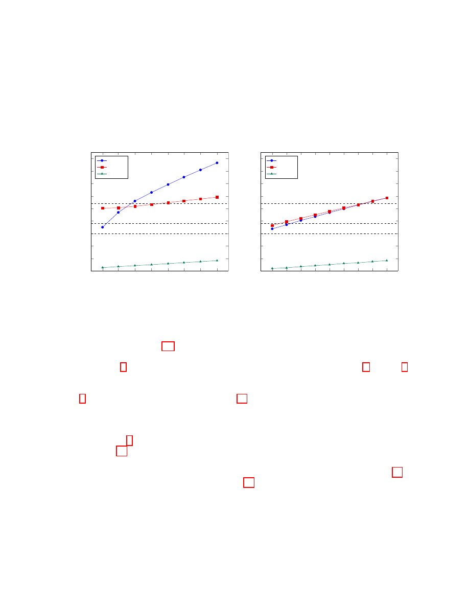
6

Choosing Parameters

One important issue with any cryptographic primitive is its efficiency for a given level of claimed
security. For public-key primitives, this can be examined by analyzing the sizes of the private and
public key, and the number of operations necessary for encryption, decryption, signing and verification.

160

314

476

638

800

954

1116

1278

20

40

60

80

100

120

140

160

180

200

19

66

145

254

394

556

755

984

k

Complexit

y

(log

2

)

Public key size (kB)

Code

Dual

Decode

(a) Encryption

306

366

426

486

546

606

666

726

786

20

40

60

80

100

120

140

160

180

200

12

17

23

30

37

46

55

65

75

k

Complexit

y

(log

2

)

Public key size (kB)

Code

Dual

Decode

(b) Signature

Fig. 3. Comparison between the complexity of decoding and the distinguishing attacks for encryption and signature.
Dashed horizontal lines denote three security levels: 2

80

, 2

96

and 2

128

.

From the analysis in Sect. 5.3 we have chosen a set of eight parameters for encryption and nine

parameters for signatures, with security levels in the range of 2

80

− 2

128

(actually slightly above 2

128

)

according to Thm. 2 . The full description of the proposed parameters are in Appx. F. In Fig. 3 we
plot comparative curves for the complexities of decoding and the complexities of the distinguishing
attacks on the code and its dual.

Fig. 4 illustrates how the complexities in Fig. 3a were calculated, by considering the fifth data

point in the graph, representing a (800, 4840) code suitable for encryption. By examining all possible
values of the attack parameter K

t

we find that the distinguishing attack on the code and its dual (a

code of dimensions (4040, 4840)) has a minimum complexity of 2

129

.

Similarly, in Fig. 5, we illustrate with a code suitable for signatures (it is the (786, 1578) code in

point eight of Fig. 3b). Again, by examining all possible values of the attack parameter K

t

we see that

the minimum complexity of the attack (on either the code or its dual (792, 1578) code) is 2

137

.

Note that the gap between the attack complexity and the complexity of decoding in Fig. 3a (the

encryption scheme) is almost a constant, and in Fig. 3b (the signature scheme) the gap is just slowly
increasing. While this can be arguably considered as a negative characteristic of the scheme, we want
to emphasize the following two arguments why we see our scheme as potentially a useful cryptographic
design: 1. The attack complexities are in the stratosphere of infeasibility of “real world” computations
in the levels of 2

80

− 2

128

(or slightly above), while the decryption complexities are in the feasible

levels of 2

23

− 2

36

; 2. Since our decoding procedure has the feature of being trivially parallelizable,

it is feasible to reduce the decoding complexity from 2

36

time units down to only a few time units.

If the same amount of parallel computing power is given to the attacker, the reduction in the attack

13

0

1,000

2,000

3,000

4,000

128

192

256

320

384

448

512

K

t

Complexit

y

(log

2

)

Code

Dual

Fig. 4. Complexity of the distinguishing attack from
Sect. 5.3 on a (800, 4840) code suitable for encryption
(and the dual (4040, 4840) code), for various choices of
K

t

.

200

300

400

500

600

700

800

128

160

192

224

256

288

320

352

K

t

Complexit

y

(log

2

)

Code

Dual

Fig. 5. Complexity of the distinguishing attack from
Sect. 5.3 on a (786, 1578) code suitable for signatures
(and the dual (792, 1578) code), for various choices of
K

t

.

complexities will be much smaller

6

, thus keeping the complexities of attacks utilizing parallelism in

the stratosphere of infeasibility .

7

Conclusions

We have introduced a cryptographic communication channel where the sender has the role of the
“noise” and can produce error vectors from an almost arbitrary big error set. For those error sets we
defined a new family of binary linear codes that with overwhelming probability can be decoded by an
efficient list decoding algorithm.

Having introduced the new codes, we constructed both encryption and signature schemes that

follow the basic structure of the McEliece scheme: G

pub

= SGP . We showed that the security of our

schemes are tightly connected to the problem of decoding a random syndrome in the Hamming metric
by providing an analog to the Information Set Decoding techniques for our error sets. Further, we
scrutinized the power of rank attacks against our scheme and that resulted to a particular choice of
parameters that offer a security in the range 2

80

− 2

128

with plausible operating characteristics.

We point out to some research directions and open questions connected with our schemes: 1.

Finding parameter sets that will offer security levels in the range of 2

256

, 2. Reducing the public key

sizes with techniques such as cyclic and MDPC codes. 3. Implementations in hardware making heavy
use of the inherent parallelism in the decoding algorithm for our codes.

References

1. Mohssen Alabbadi and Stephen B. Wicker. Cryptanalysis of the Harn and Wang modification of the Xinmei digital

signature scheme. In Electronics Letters 28,, pages 1756–1758, 1992. (Cited on page 3.)

2. Mohssen Alabbadi and Stephen B. Wicker. Security of Xinmei digital signature scheme. In Electronics Letters 28,,

pages 890–891, 1992. (Cited on page 3.)

3. Mohssen Alabbadi and Stephen B. Wicker. A digital signature scheme based on linear error-correcting block codes. In

Josef Pieprzyk and Reihanah Safavi-Naini (editors). Advances cryptology-ASIACRYPT ’94. Proceedings of the Fourth
International Conference held at the University of Wollongong, Wollongong, November 28-December 1, Lecture Notes
Computer Science 917. Springer, pages 238–248, 1994. (Cited on page 3.)

4. D. Angluin and L.G. Valiant. Fast probabilistic algorithms for hamiltonian circuits and matchings. J. of Computer

and System Sciences, 19:155–193, 1979. (Cited on page 6.)

6

Decoding procedures use much simpler matrix-vector multiplications, while the rank attacks have to perform infeasible
number of more expensive operations of matrix rank computations.

14

5. M. Baldi, F. Chiaraluce, R. Garello, and F. Mininni. Quasi-cyclic low-density parity-check codes in the mceliece

cryptosystem. In Communications, 2007. ICC ’07. IEEE International Conference on, pages 951–956, 2007. (Cited
on page 3.)

6. Anja Becker, Antoine Joux, Alexander May, and Alexander Meurer. Decoding random binary linear codes in 2n/20:

how 1 &#43; 1 = 0 improves information set decoding. In Proceedings of the 31st Annual international conference on
Theory and Applications of Cryptographic Techniques, EUROCRYPT’12, pages 520–536, Berlin, Heidelberg, 2012.
Springer-Verlag. (Cited on pages 3, 10, and 20.)

7. Elwyn Berlekamp, Robert J. McEliece, and Henk C. A. Van Tilborg. On the inherent intractability of certain coding

problems. Information Theory, IEEE Transactions on, 24(3):384–386, 1978. (Cited on page 22.)

8. D. Bernstein, T. Lange, and C. Peters. Attacking and defending the mceliece cryptosystem. Post-Quantum Cryp-

tography, pages 31–46, 2008. (Cited on page 3.)

9. Daniel J. Bernstein. List decoding for binary goppa codes. In Coding and cryptology—third international workshop,

IWCC 2011, Qingdao, China, May 30–June 3, 2011, proceedings, edited by Yeow Meng Chee, Zhenbo Guo, San
Ling, Fengjing Shao, Yuansheng Tang, Huaxiong Wang, and Chaoping Xing, Lecture Notes Computer Science 6639,
Springer, 2011. ISBN 978-3-642-20900-0., pages 62–80, 2011. (Cited on page 3.)

10. Daniel J. Bernstein. Simplified high-speed high-distance list decoding for alternant codes. In Post-Quantum Cryp-

tography 4th International Workshop, PQCrypto 2011, Taipei, Taiwan, November 29 December 2, 2011, proceedings
Lecture Notes Computer Science 7071. Springer., pages 200–216, 2011. (Cited on page 3.)

11. Daniel J. Bernstein, Tanja Lange, and Christiane Peters. Smaller decoding exponents : ball-collision decoding. In

CRYPTO 2011, Lecture Notes Computer Science, Vol. 6841. Springer-Verlag Berlin-Heidelberg, 2011, pages 743–760,
2011. (Cited on page 3.)

12. Daniel J. Bernstein, Tanja Lange, and Christiane Peters. Smaller decoding exponents: ball-collision decoding. In

Proceedings of the 31st annual conference on Advances in cryptology, CRYPTO’11, pages 743–760, Berlin, Heidelberg,
2011. Springer-Verlag. (Cited on pages 3, 10, and 20.)

13. Daniel J. Bernstein, Tanja Lange, and Christiane Peters. Wild McEliece incognito. In Post-Quantum Cryptography,

Fourth international workshop, PQCrypto 2011, Lecture Notes Computer Science 7071, Springer., pages 244–254,
2011. (Cited on page 3.)

14. Pierre-Louis Cayrel, Ayoub Otmani, and Damien Vergnaud. On kabatianskii-krouk-smeets signatures. In Interna-

tional Workshop on the Arithmetic of Finite Fields, WAIFI 2007, Springer, Lecture Notes Computer Science, volume
4547, pages 237–251, 2007. (Cited on page 3.)

15. H. Chernoff. Asymptotic efficiency for tests based on the sum of observations. Ann. Math. Stat., 23:493–507, 1952.

(Cited on page 6.)

16. Nicolas Courtois, Matthieu Finiasz, and Nicolas Sendrier. How to achieve a McEliece-based digital signature scheme.

In Colin Boyd, editor, ASIACRYPT 2001, volume 2248 of Lecture Notes in Computer Science, pages 157–174.
Springer, 2001. (Cited on pages 3 and 5.)

17. W. Diffie and M. Hellman. New directions in cryptography. IEEE Transactions on Information Theory, 22(6):644–

654, November 1976. (Cited on page 3.)

18. P. Elias. List decoding for noisy channels, technical report 335. Technical report, Research Laboratory of Electronics,

MIT, 1957. (Cited on pages 3 and 6.)

19. Jean-Charles Faug`

ere. A new efficient algorithm for computing Gr¨

obner bases (F4). Journal of Pure and Applied

Algebra, 139(1–3):61–88, June 1999. (Cited on page 19.)

20. Matthieu Finiasz and Nicolas Sendrier. Security bounds for the design of code-based cryptosystems. In Proceedings of

the 15th International Conference on the Theory and Application of Cryptology and Information Security: Advances
in Cryptology, ASIACRYPT ’09, pages 88–105, Berlin, Heidelberg, 2009. Springer-Verlag. (Cited on pages 3, 10,
and 20.)

21. Ernst M. Gabidulin, A. V. Paramonov, and O. V. Tretjakov. Ideals over a non-commutative ring and their ap-

plications to cryptography. In D. W. Davies, editor, Advances cryptology-EUROCRYPT ’91. Proceedings of the
Workshop on the Theory and Application of Cryptographic Techniques held Brighton, April 8-11, Lecture Notes
Computer Science 547. Springer ISBN 3-540-54620-0, pages 482–489, 1991. (Cited on page 3.)

22. Philippe Gaborit. Shorter keys for code based cryptography. In WCC 2005, Oyvind Ytrehus, Springer, Lecture Notes

Computer Science, volume 3969, pages 81–90, 2005. (Cited on page 3.)

23. Venkatesan Guruswami and Madhu Sudan. Improved decoding of reed-solomon and algebraic-geometric codes. In

FOCS, pages 28–39. IEEE Computer Society, 1998. (Cited on pages 3 and 6.)

24. L. Harn and D. C. Wang. Cryptanalysis and modification of digital signature scheme based on error-correcting codes.

In Electronics Letters 28, pages 157–159, 1992. (Cited on page 3.)

25. Heeralal Janwa and Oscar Moreno. McEliece public key cryptosystems using algebraic-geometric codes. In Designs,

Codes and Cryptography 8, pages 293–307, 1996. (Cited on page 3.)

26. S. M. Johnson. A new upper bound for error-correcting codes. IRE Transactions on Information Theory, IT-8:203–

207, 1962. (Cited on page 6.)

15

27. Gregory Kabatianskii, E. Krouk, and Ben Smeets. A digital signature scheme based on random error-correcting

codes. In Michael Darnell, editor, Cryptography and coding. Proceedings of the 6

th

IMA International Conference

held at the Royal Agricultural College, Cirencester, December 17-19, Lecture Notes Computer Science 1355. Springer,
pages 161–177, 1997. (Cited on page 3.)

28. P. J. Lee and E. F. Brickell. An observation on the security of mceliece’s public-key cryptosystem. In Lecture

Notes in Computer Science on Advances in Cryptology-EUROCRYPT’88, pages 275–280, New York, NY, USA,
1988. Springer-Verlag New York, Inc. (Cited on pages 3, 10, and 20.)

29. J. S. Leon. A probabilistic algorithm for computing minimum weights of large error-correcting codes. IEEE Trans.

Inf. Theor., 34(5):1354–1359, September 2006. (Cited on page 10.)

30. Yuan Xing Li and Chuanjia Liang. A digital signature scheme constructed with error-correcting codes. In Chinese

: Acta Electronica Sinica 19, pages 102–104, 1991. (Cited on page 3.)

31. MAGMA. High performance software for algebra, number theory, and geometry — a large commercial software

package. (Cited on page 19.)

32. Alexander May, Alexander Meurer, and Enrico Thomae. Decoding random linear codes in &#213;(20.054n). In

Proceedings of the 17th international conference on The Theory and Application of Cryptology and Information
Security, ASIACRYPT’11, pages 107–124, Berlin, Heidelberg, 2011. Springer-Verlag. (Cited on pages 3, 10, and 20.)

33. R. J. McEliece. A Public-Key System Based on Algebraic Coding Theory, pages 114–116. Jet Propulsion Lab, 1978.

DSN Progress Report 44. (Cited on page 3.)

34. Rafael Misoczki, Jean-Pierre Tillich, Nicolas Sendrier, and Paulo S. L. M. Barreto. Mdpc-mceliece: New mceliece

variants from moderate density parity-check codes. IACR Cryptology ePrint Archive, 2012:409, 2012. informal
publication. (Cited on page 3.)

35. C. Monico, J. Rosenthal, and A. Shokrollahi. Using low density parity check codes in the mceliece cryptosystem. In

Information Theory, 2000. Proceedings. IEEE International Symposium on, pages 215–, 2000. (Cited on page 3.)

36. Harald Niederreiter. Knapsack-type cryptosystems and algebraic coding theory. In Problems of Control and Infor-

mation Theory 15, pages 159–166, 1986. (Cited on page 3.)

37. E. Prange. The use of information sets in decoding cyclic codes. IRE Transactions on Information Theory, 8:5–9,

1962. (Cited on page 10.)

38. R.L. Rivest, A. Shamir, and L. Adelman. A method for obtaining digital signatures and public-key cryptosystems.

Communications of the ACM, 21(2):120–126, 1978. (Cited on page 3.)

39. V.M. Sidelnikov. A public-key cryptosystem based on binary Reed-Muller codes. Discrete Math. Appl., 4(3):1, 1994.

(Cited on page 3.)

40. Jacques Stern. A method for finding codewords of small weight. In Proceedings of the 3rd International Colloquium

on Coding Theory and Applications, pages 106–113, London, UK, UK, 1989. Springer-Verlag. (Cited on pages 3, 10,
and 20.)

41. Madhu Sudan. Decoding of Reed Solomon codes beyond the error-correction bound. Journal of Complexity, 13:180–

193, 1997. (Cited on page 3.)

42. Johan van Tilburg. Cryptanalysis of the alabbadi-wicker digital signature scheme. In Proceedings of Fourteenth

Symposium on Information Theory in the Benelux, pages 114–119, 1993. (Cited on page 3.)

43. Xinmei Wang. Digital signature scheme based on error-correcting codes. In Electronics Letters, volume 26, pages

898–899, 1990. (Cited on page 3.)

44. J. M. Wozencraft. List decoding. quarterly progress report. Technical report, Research Laboratory of Electronics,

MIT, 1958. (Cited on pages 3 and 6.)

45. Sheng-Bo Xu, Jeroen Doumen, and Henk C. A. van Tilborg. On the security of digital signature schemes based on

error-correcting codes. In Designs, Codes and Cryptography, volume 28, pages 187–199, 2003. (Cited on page 3.)

16

A

Proofs

A.1

Proof of Proposition 1

Proof. 1. D(E

l

1

× E

l

2

) = |E

l

1

× E

l

2

|

1/(l

1

+l

2

)

= (|E

l

1

| · |E

l

2

|)

1/(l

1

+l

2

)

= (ρ

l

1

· ρ

l

2

)

1/(l

1

+l

2

)

= ρ.

2. Follows directly from 1.

A.2

Proof of Proposition 2

Proof. 1. Since D(E) = ρ, we have that |E| = ρ

n

, and thus |W

E

| = ρ

n

. From here it follows that the

probability that a random word is in the set W

E

is p = ρ

n

/2

n

. We can consider the event that one

codeword is in the set W

E

as independent from the event that another codeword is in W

E

. There

are 2

k

codewords, so it follows directly that the expected number of codewords in W

E

is ρ

n

2

k−n

.

For the second part, let N = 2

k

and fix an enumeration c

1

, c

2

, . . . c

N

of C. By letting the random

variables X

i

be 1 iff c

i

∈ W

E

in Lemma 1, and setting = 1 − 1/(2pN ) in (2), the claim follows.

2. In this situation we again have a sequence of independent events. Now, the number of codewords

except c is 2

k

− 1, and the probability that a random word except c is in the set W

E

\ {c} is

p = (ρ

n

−1)/(2

n

−1). Now the expected number of codewords in W

E

\{c} is (ρ

n

−1)(2

k

−1)/(2

n

−1)

which can be approximated to ρ

n

2

k−n

for large enough n and k.

The second part follows directly from Lemma 1, by setting = 1/(2pN ) − 1 in (3).

A.3

Proof of Proposition 3

Proof. Let i ∈ {1, . . . , w}. Then, from Proposition 2 the condition E[|L

i−1

|] ≥ E[|L

i

|] turns into

ρ

n

1

+k

1

+···+n

i−1

+k

i−1

2

(k

1

+···+k

i−1

)−(n

1

+k

1

+...n

i−1

+k

i−1

)

≥

≥ ρ

n

1

+k

1

+···+n

i−1

+k

i−1

+n

i

+k

i

2

(k

1

+···+k

i−1

+k

i

)−(n

1

+k

1

+...n

i−1

+k

i−1

+n

i

+k

i

)

which in turn is equivalent to

2

n

i

≥ ρ

n

i

+k

i

and further, equivalent to

n

i

≥ k

i

log

2

ρ

1 − log

2

ρ

.

A.4

Proof of Proposition 4

Proof. 1. In each step of the Alg. 3, Phase 1, we need to find a valid extension of the error by picking

a valid part of length k

i

and then validating it on the remaining n

i

bits. The probability that the

n

i

bits, when the corresponding part of x is evaluated, to give a valid error extension is

(

|E|

2

l

)

n

i

/`

= (

ρ

2

)

n

i

Hence, we need approximately ExpLimit

i

≈ (2/ρ)

n

i

tries in order to find a valid error extension.

2. Since the List decoding for producing signatures starts in the last block, the claim follows directly

from Proposition 2.

17

A.5

Proof of Theorem 2

Proof. We will evaluate the complexity of the attack on the generator matrix of the code. The attack
on the dual code is analogous.

First of all, lets emphasize that Step 1 has the biggest complexity, so we can WLOG omit the other

steps from our complexity estimation.

First, let’s consider a more general strategy of choosing in the attack. Suppose we first choose m/`

blocks, K

t

< m < n out of the possible n/` in the hope that, among them there are K

t

/` + 1 blocks

with smaller rank than K

t

+ `. The probability of this to happen is

P r

m

=

m/`

K

t

/` + 1

!

n/` − m/`

N

t

/` − (K

t

/` + 1)

!

n/`

N

t

/`

!

−1

(13)

Suppose the choice was made correctly. Now the cost of finding the K

t

/` + 1 blocks of smaller rank

among the m/` is

Cost

m

=

m/`

K

t

/` + 1

!

· Cost

rank

Hence, the total amount of work is

Dist

m

= P r

−1

m

· Cost

m

=

n/`

N

t

/`

!

n/` − m/`

N

t

/` − (K

t

/` + 1)

!

−1

· Cost

rank

Since m/` ≥ (K

t

/` + 1), the minimum complexity is obtained for m = K

t

/` + 1. From here we get

that

P r

K

t

/`+1

= P r

rank

=

n/` − (K

t

/` + 1)

N

t

/` − (K

t

/` + 1)

!

n/`

N

t

/`

!

−1

(14)

and

Cost

K

t

/`+1

= Cost

rank

The rank computation takes approximately Cost

rank

= k(K

t

+ `)

ω−1

operations, where ω is the linear

algebra constant.

As we said, the same strategy applies for the dual code, for which instead of K

t

we have N

t

− K

t

.

Now the claim follows directly.

The parameter t is an optimization parameter for the attack, and its optimal value depends strongly

on the chosen parameters. We should note that, for the sets of parameters that we use, because of the
nature of the curve of the complexity for different K

t

, the best strategies are always for either t = 1

or t = w − 1.

B

An Example of the Modeling of ρISD using Polynomial System Solving

Let E

`

be an error set of density ρ = 3

1/2

and granulation ` = 2. Without loss of generality, we

can assume that E

`

= {(00), (01), (10)}. Let (e

1

, e

2

) ∈ E

`

. Then, the equation e

1

e

2

= 0 describes

completely the error set E

`

. Hence, the system (8) turns into:

(x

1

, . . . , x

k

)G

pub

+ (y

1

, . . . , y

n

) = c

y

1

y

2

= 0

. . .

y

n−1

y

n

= 0

18

The system can be easily transformed to the following form:

A

1

(x

1

, . . . , x

k

)A

2

(x

1

, . . . , x

k

) = 0

. . .

(15)

A

n−1

(x

1

, . . . , x

k

)A

n

(x

1

, . . . , x

k

) = 0

where A

i

are some affine expressions in the variables x

1

, . . . , x

k

.

We can introduce an optimization parameter p as follows. Suppose we have made a correct guess

that the equation y

2t−1

+ y

2t

= b

t

, b

t

∈ {0, 1} holds for p pairs (y

2t−1

, y

2t

) of coordinates of the error

vector. Adding these p new equations to the system reduces the complexity of solving it. Note that
it is enough to correctly guess k equation to obtain a full system of k unknowns. The probability of
making the correct guess is P r = (2/3)

p

. Under the natural constrain 0 ≤ p ≤ k, we can roughly

estimate the complexity to

Comp = (2/3)

p

·

k − p

Dreg

k−p

!

+ p

!

ω

where Dreg

k−p

denotes the degree of regularity of a system of k − p variables of the form (15).

We performed some experiments using the F

4

algorithm [19] implemented in MAGMA [31], and

based on rather conservative projections of the degree of regularity, we give the following table with a
rough estimate of the lower bound of the complexity.

Table 2. Estimated complexity of solving ρISD using the F

4

algorithm for ` = 2, ρ = 3

1/2

.

k

Complexity

128

2

84

256

2

152

512

2

237

C

Adaptions of ISD to Generalized Error Sets

Let ρISD

V AR

denote the complexity of some variant of the ISD algorithms adapted to error sets of

density ρ. Then as usual, we can write:

ρISD

V AR

= ρP r

−1

V AR

· ρCost

V AR

where ρP r

V AR

is the probability of success of one iteration of the algorithm, and ρCost

V AR

denotes

the cost of each of the iterations. We summarize the results of adapting several ISD variants in the
following theorem.

Theorem 3. The probability of success of one iteration and the cost of one iteration of the Lee-Brickell
variant, Stern variant, Finiasz-Sendrier variant, Bernstein-Lange-Peters variant, May-Meurer-Thomae
variant and Becker-Joux-May-Meurer variant adapted to error sets of density ρ are given in Table 3.

Proof (sketch). We first note that all the parameters and the strategy used in the presented variants
ρISD

V AR

is the same as in the original algorithms ISD

V AR

. The main difference is in the probability

of success and the size of the constructed lists.

19

In the original variants, one allows a certain amount of errors to appear in the coordinates indexed

by the information set I in a specific pattern. Also, a specific number of errors is allowed on certain
coordinates outside I. Each and every new algorithm uses different pattern, carefully chosen in order
to increase the probability of having such a particular pattern compared to previous variants.

Without loss of generality, let ˜

k be the size of some fixed portion of the coordinates. From the

discussion at the beginning of the section, we see that unlike in the standard ISD

V AR

, in ρISD

V AR

the probability of “guessing” the pattern in p blocks does not depend on n, or the structure of the

error vector outside the fixed coordinates. It is always given by

˜

k/`

p

(

ρ

`

−1

)

p

ρ

˜

k

. This probability can be

used to compute the probability of any of the variants.

Now, assuming that the pattern is correctly guessed, one forms one or more lists of size p subsets

of the fixed coordinates, in order to match a computed tag to another, using plain or collision type

of matching. In our case, the number of such subsets is given by

˜

k/`

p

ρ

`

− 1

p

, where

˜

k/`

p

is the

number of size p subsets of blocks of length `, and

ρ

`

− 1

is the number of possible error patterns

inside a block where we allow to have not guessed the pattern. Using this formula we can compute the
size of the created lists in the algorithms of all variants. The particular details are left to the reader.

Table 3. Complexity of ISD variants adapted to error sets of density ρ. Cost

Gauss

denotes the complexity of Gaussian

elimination. The meaning of the optimizing parameters in each of the formulas below can be found in [28,40,20,12,32,6].

Variant

ρP r

V AR

ρCost

V AR

− Cost

Gauss

LB

k/`

p

(ρ

`

−1)

p

ρ

k

k/`

p

(ρ

`

− 1)

p

pn

ST

k/2`

p

2 (ρ

`

−1)

2p

ρ

k+λ

2λpL + 2pn

L

2

2

λ

,

L =

k/2`

p

(ρ

`

− 1)

p

F S

(k+λ)/2`

p

2 (ρ

`

−1)

2p

ρ

k+λ

2λpL + 2pn

L

2

2

λ

,

L =

(k+λ)/2`

p

(ρ

`

− 1)

p

BLP

k/2`

p

2 λ

1

/`

q

λ

2

/`

q

k/2`

p

(ρ

`

− 1)

p

2(λ

1

+ λ

2

)p +

k/2`

p

λ

1

/`

q

+

λ

2

/`

q

(ρ

`

− 1)

p+q

(λ

1

+ λ

2

)q

·

(ρ

`

−1)

2p+2q

ρ

k+λ1+λ2

+

(

k/2`

p

)

2

(

λ1/`

q

)(

λ2/`

q

)

(ρ

`

−1)

2p+2q

2

λ1+λ2

2(p + q)n

M M T

(k+λ)/2`

p

2 (ρ

`

−1)

2p

ρ

k+λ

2λ

2

pL + (2n + λ − λ

2

)p

L

2

2

λ2

+ pn

L

4

2

λ+λ2

,

L =

(k+λ)/2`

p/2

(ρ

`

− 1)

p/2

BJ M M

(k+λ)/`

p

(ρ

`

−1)

p

ρ

k+λ

4P r

−4
coll

p

2

L

3

log

2

R

2

+ n

L

2
3

R

2

+ 2n

p

1

L

2
2

R

2

R

1

+ p

L

2
1

R

1

2

λ

,

P r

coll

=

(k+λ)/2`

p

2

/2

2 (k+λ)/`

p

2

−1

, p

i

=

p

i−1

2

+

i

, i = 1, 2, p

0

= p,

L

i

=

(k+λ)/2`

p

i

(ρ

`

− 1)

p

i

, i = 1, 2,

L

3

=

(k+λ)/2`

p

2

/2

(ρ

`

− 1)

p

2

/2

,

R

i

=

p

i−1

p

i−1

/2

(k+λ)/`−p

i−1

i

(ρ

`

− 1)

i

, i = 1, 2, p

0

= p

20

D

Small Decoding Example

In this example we consider a binary (24, 6) code generated by:

G =












1

0 1 0 0 0 1 0 0 0 1 0 1 0 0 0 1 1 0

1

0 0 1 1 0 1 0 1 0 1 0 0 0 1 0 0 0 0

1

1 1 0 1 0 1 0 0 0 0 1 0 0 1 0 0 0 1

1

0 0 1 1 1 0 1 0 1 1 0 1 1 0 1 0 0 1

1

0 1 1 1 1 1 1 1 1 0 1 1

1

1 1 0 0 1 1












.

(16)

In particular, we have k

1

= 4, k

2

= 1, k

3

= 1 and n

1

= n

2

= n

3

= 6 (ref. (4)). Let E

`

= {00, 01, 10}

be our error set, having granulation ` = 2 and density ρ = 3

1/2

. For the following values of the message

x and error vector e, we obtain the codeword y.

x = (101001),

(17)

e = (100110 000001 101010 000000),

(18)

y = xG + e = (

y

0

z

}|

{

001111

y

1

z

}|

{

100101

y

2

z

}|

{

101101

y

3

z

}|

{

100100).

(19)

We now decode y using Alg. 1.

Step 0: Here we simply calculate all possible decodings of the first four bits of y

0

, by adding to it all

possible error vectors in four bits. This yields the following T

0

:

T

0

= {(0011), (0111), (1011), (0010), (0110), (1010), (0001), (0101), (1001)}.

Step 1 - Step 3: Next, we try to remove all vectors in T

0

that does not satisfy (5).

To illustrate the optimization proposed in Remark 1, we look at the processing of the element

x

0

= (0011) from T

0

in detail through Step 1. As mentioned in the remark, initially we only consider

the first two columns of B

1

when trying to determine the validity of x

0

. That is, we test the following

restricted variant of (5):

(x

0

B

1

)[1 . . . 2] + e

0

[1 . . . 2]

?

= y

1

[1 . . . 2],

for some e

0

∈ E

k

1

/`

.

With the concrete values of x

0

, y

1

and B

1

as given above, this becomes:

(0011)








0 1
0 0
1 1
0 0








+ e

0

[1 . . . 2] = (11) + e

0

[1 . . . 2] = (10).

By inspection we see that an error of the form (01XXXX) will satisfy this equation, so we continue

with the next two columns of B

1

:

(0011)








0 1 0 0
0 0 1 1
1 1 0 1
0 0 1 1








+ e

0

[1 . . . 4] = (1110) + e

0

[1 . . . 4] = (1001).

21

At this point we see that there are no errors that satisfies this equation (since it would have to be of
the form (0111XX) which is not a valid error in our error set). Hence, we can discard x

0

immediately,

without considering all of B

1

. Applying the same technique to the rest of the elements of T

0

we obtain:

L

1

= {(0010), (1010), (0101)}.

From the elements in L

1

we build up the temporary list T

1

of all possible decodings of y

0

having

length 4 + 1 = 5:

T

1

= {x

0

k (y

0

[5] + e

0

) | x

0

∈ L

1

, e

0

∈ E

k

2

/`

}

= {(00100), (00101), (10100), (10101), (01010), (01011)}.

Repeating the above process for Step 2 and Step 3, we obtain the lists L

2

and L

3

:

L

2

= {(10100), (01010)}

L

3

= {(101001)}.

Thus, in this case we obtain a unique decoding.

E

NP-completeness of Decoding General Error Sets

If C is an (n, k) binary linear code and y a received vector, the general decoding problem asks to
find the codeword that most likely was sent. That is, “most-likely” means to find an error vector e
of minimal weight, such that x = y + e is word in the code. Equivalently, if H is the (n − k) × n
parity-check matrix of C, the problem can be stated as asking to find a minimal weight solution e

0

to

the equation s = eH

T

, where s is the syndrome yH

T

.

The hardness of decoding arbitrary linear codes have long been established based on the decades of

efforts trying to solve it. Furthermore, Berlekamp et al. [7], showed that the related decisional problem,
COSET WEIGHTS, is NP-complete:

Definition 2 (COSET WEIGHTS).

Input: A binary (n − k) × n matrix H, a binary vector s ∈ F

n−k
2

, and a non-negative integer w.

Output: YES, if there exists a vector e of Hamming weight ≤ w such that eH

T

= s. NO otherwise.

We now show that the problem of decoding arbitrary linear codes when using the error sets defined

in Def. 1 is NP-complete.

Definition 3 (ERROR SETS).

Input: A binary (n − k) × n matrix H, a binary vector s ∈ F

n−k
2

, and a generalized error set E

`

⊂ F

`

2

.

Output: YES, if there exists an error vector e ∈ E

m

`

such that eH

T

= s. NO otherwise.

Proving ERROR SETS NP-complete amounts to nothing more than noting that the set of errors

having Hamming weight ≤ w constitutes a generalized error set. That is, COSET WEIGHTS is simply
a special case of ERROR SETS by letting ` = n and

E

`

= Ker({

Y

i∈I⊆[n]

x

i

∈ F

2

[x

1

, . . . , x

n

] | |I| > w}) = {e ∈ F

n
2

| wt(e) ≤ w},

(20)

Thus, since a solution to ERROR SETS would be a solution to COSET WEIGHTS, we have proved

Thm. 1.

22

F

Full Description of Sets of Parameters for Security Levels in the Range of
2

80

− 2

128

We denote with K = (k

1

, . . . , k

w

) and with N = (n

1

, . . . , n

w

) the vectors of values used in definition

of concrete generator matrices as defined in equation (4). The used error set for all concrete codes is
E

2

= {x ∈ F

2

2

| wt(x) < 2} = {(0, 0), (0, 1), (1, 0)}, thus ` = 2. For computing the complexities of the

rank attacks on the code and on its dual code we use equation (12), and we give here the values for
K

t

/` and N

t

/` for which those complexities are achievable.

Codes for encrytion

1. Code (1160, 160).

Public key size: 19.53 Kb.
w = 17, K = (32, 8, 8, . . . , 8), N = (32, 32, . . . , 32, 488).
Decoding complexity: 2

25.36

.

Best rank attack complexity: 2

90

for K

t

/` = 152 and N

t

/` = 664.

The dual code is (1160, 1000).
Best dual code rank attack complexity: 2

120.61

for K

t

/` = 968 and N

t

/` = 1096.

2. Code (2050, 314).

Public key size: 66.54 Kb.
w = 36, K = (34, 8, 8, . . . , 8), N = (32, 32, . . . , 32, 616).
Decoding complexity: 2

26.94

.

Best rank attack complexity: 2

113.75

for K

t

/` = 306 and N

t

/` = 1426.

The dual code is (2050, 1736).
Best dual code rank attack complexity: 2

121.20

for K

t

/` = 1704 and N

t

/` = 1984.

3. Code (2980, 476).

Public key size: 145.50 Kb.
w = 56, K = (36, 8, 8, . . . , 8), N = (32, 32, . . . , 32, 744).
Decoding complexity: 2

28.53

.

Best rank attack complexity: 2

131.96

for K

t

/` = 36 and N

t

/` = 68.

The dual code is (2980, 2504).
Best dual code rank attack complexity: 2

123.61

for K

t

/` = 2472 and N

t

/` = 2912.

4. Code (3910, 638).

Public key size: 254.83 Kb.
w = 76, K = (38, 8, 8, . . . , 8), N = (32, 32, . . . , 32, 872).
Decoding complexity: 2

30.11

.

Best rank attack complexity: 2

145.80

for K

t

/` = 38 and N

t

/` = 70.

The dual code is (3910, 3272).
Best dual code rank attack complexity: 2

126.44

for K

t

/` = 3240 and N

t

/` = 3840.

5. Code (4840, 800).

Public key size: 394.53 Kb.
w = 96, K = (40, 8, 8, . . . , 8), N = (32, 32, . . . , 32, 1000).
Decoding complexity: 2

31.70

.

Best rank attack complexity: 2

158.51

for K

t

/` = 40 and N

t

/` = 72.

The dual code is (4840, 4040).
Best dual code rank attack complexity: 2

129.37

for K

t

/` = 4008 and N

t

/` = 4768.

23

6. Code (5730, 954).

Public key size: 556.19 Kb.
w = 115, K = (42, 8, 8, . . . , 8), N = (32, 32, . . . , 32, 1128).
Decoding complexity: 2

33.28

.

Best rank attack complexity: 2

170.30

for K

t

/` = 42 and N

t

/` = 74.

The dual code is (5730, 4776).
Best dual code rank attack complexity: 2

132.36

for K

t

/` = 4744 and N

t

/` = 5656.

7. Code (6660, 1116).

Public key size: 755.26 Kb.
w = 135, K = (44, 8, 8, . . . , 8), N = (32, 32, . . . , 32, 1256).
Decoding complexity: 2

34.86

.

Best rank attack complexity: 2

181.88

for K

t

/` = 44 and N

t

/` = 76.

The dual code is (6660, 5544).
Best dual code rank attack complexity: 2

135.27

for K

t

/` = 5512 and N

t

/` = 6584.

8. Code (7590, 1278).

Public key size: 984.71 Kb.
w = 155, K = (46, 8, 8, . . . , 8), N = (32, 32, . . . , 32, 1384).
Decoding complexity: 2

36.45

.

Best rank attack complexity: 2

193.15

for K

t

/` = 46 and N

t

/` = 78.

The dual code is (7590, 6312).
Best dual code rank attack complexity: 2

138.17

for K

t

/` = 6280 and N

t

/` = 7512.

Codes for signatures

1. Code (650, 306).

Public key size: 12.85 Kb.
w = 6, K = (84, 48, 48, 48, 48, 30), N = (48, 48, 48, 48, 48, 104).
Decoding complexity: 2

23.77

.

Best rank attack complexity: 2

87.54

for K

t

/` = 276 and N

t

/` = 516.

The dual code is (650, 344).
Best dual code rank attack complexity: 2

93.32

for K

t

/` = 296 and N

t

/` = 518.

2. Code (766, 366).

Public key size: 17.87 Kb.
w = 7, K = (94, 48, . . . , 48, 32), N = (48, 48, . . . , 48, 112).
Decoding complexity: 2

25.36

.

Best rank attack complexity: 2

94.44

for K

t

/` = 334 and N

t

/` = 622.

The dual code is (766, 400).
Best dual code rank attack complexity: 2

98.93

for K

t

/` = 352 and N

t

/` = 624.

3. Code (882, 426).

Public key size: 23.71 Kb.
w = 8, K = (104, 48, . . . , 48, 34), N = (48, 48, . . . , 48, 120).
Decoding complexity: 2

26.94

.

Best rank attack complexity: 2

101.00

for K

t

/` = 392 and N

t

/` = 728.

The dual code is (882, 456).
Best dual code rank attack complexity: 2

104.48

for K

t

/` = 408 and N

t

/` = 730.

24

4. Code (998, 486).

Public key size: 30.37 Kb.
w = 9, K = (114, 48, . . . , 48, 36), N = (48, 48, . . . , 48, 128).
Decoding complexity: 2

28.53

.

Best rank attack complexity: 2

107.36

for K

t

/` = 450 and N

t

/` = 834.

The dual code is (998, 512).
Best dual code rank attack complexity: 2

110.00

for K

t

/` = 464 and N

t

/` = 836.

5. Code (1114, 546).

Public key size: 37.86 Kb.
w = 10, K = (124, 48, . . . , 48, 38), N = (48, 48, . . . , 48, 136).
Decoding complexity: 2

30.11

.

Best rank attack complexity: 2

113.55

for K

t

/` = 508 and N

t

/` = 940.

The dual code is (1114, 568).
Best dual code rank attack complexity: 2

115.48

for K

t

/` = 520 and N

t

/` = 942.

6. Code (1230, 606).

Public key size: 46.16 Kb.
w = 11, K = (134, 48, . . . , 48, 40), N = (48, 48, . . . , 48, 144).
Decoding complexity: 2

31.69

.

Best rank attack complexity: 2

119.63

for K

t

/` = 566 and N

t

/` = 1046.

The dual code is (1230, 624).
Best dual code rank attack complexity: 2

120.93

for K

t

/` = 576 and N

t

/` = 1048.

7. Code (1346, 666).

Public key size: 55.28 Kb.
w = 12, K = (144, 48, . . . , 48, 42), N = (48, 48, . . . , 48, 152).
Decoding complexity: 2

33.28

.

Best rank attack complexity: 2

125.61

for K

t

/` = 624 and N

t

/` = 1152.

The dual code is (1346, 680).
Best dual code rank attack complexity: 2

126.34

for K

t

/` = 632 and N

t

/` = 1154.

8. Code (1462, 726).

Public key size: 65.23 Kb.
w = 13, K = (154, 48, . . . , 48, 44), N = (48, 48, . . . , 48, 160).
Decoding complexity: 2

34.87

.

Best rank attack complexity: 2

131.52

for K

t

/` = 682 and N

t

/` = 1258.

The dual code is (1462, 736).
Best dual code rank attack complexity: 2

131.74

for K

t

/` = 688 and N

t

/` = 1260.

9. Code (1578, 786).

Public key size: 75.99 Kb.
w = 14, K = (164, 48, . . . , 48, 46), N = (48, 48, . . . , 48, 168).
Decoding complexity: 2

36.45

.

Best rank attack complexity: 2

137.37

for K

t

/` = 740 and N

t

/` = 1364.

The dual code is (1578, 792).
Best dual code rank attack complexity: 2

137.11

for K

t

/` = 744 and N

t

/` = 1366.

25