Summer School: ENERGY SUPPLY FOR MODERN BUILDINGS, 21 - 24.09.2004, Gliwice, POLAND

Jacek KALINA

Institute of Thermal Technology, Silesian University of Technology, Poland
Konarskiego 22, 44-101 Gliwice
tel.: [phone]; fax: [phone]
e-mail: [e-mail]

ENERGY FOR BUILDINGS - ESTIMATION OF DEMAND VARIATIONS AND

MODERN SYSTEMS OF ENERGY SUPPLY

Abstract. Paper presents problems that have to be typically solved when local, built-in energy supply
system is being planned for a building. The material is divided into two parts. The first part gives an
overview of an estimation of energy demand and particular load variations in time. The second part is
dedicated to the plant sizing procedure and optimization techniques. The most important problems of
planning the energy supply systems for buildings are being outlined and discussed.

1. Energy in buildings – introduction

It is being estimated that the sector of buildings consumes about 40% of the global energy

consumption. This figure vary form country to country but generally buildings can be
regarded as one of the most important energy user. If we take into account that the most of
energy today comes from fossil fuels it can be found that buildings are also responsible for a
quite impressive emission of pollutants.

Any action undertaken in the area of energy savings in the sector of buildings globally

leads to favourable energy, ecological and economic effects. One of the best way to save
energy and emission is precise, detailed and reliable design of energy supply systems. On the
other hand the design process requires many data from building for which the energy system
is being planned. The more detailed information we have, the more perfect system we are able
to design.

The total energy demand at any building can be divided at least into two forms of final

energy: heat and electricity. In most cases the more detailed classification can be made. The
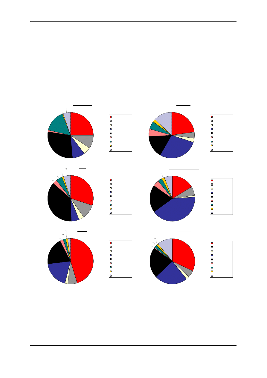
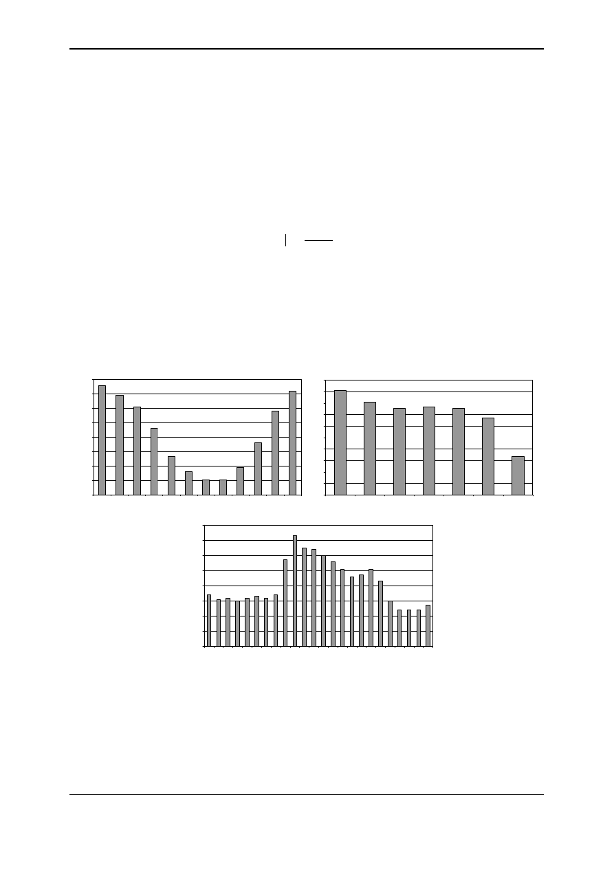
analysis of energy consumption in the main types of buildings is shown in figure 1. The
figures presented had been worked out by the Office of Energy Efficiency and Renewable
Efficiency of U.S. Department of Energy.

The most important forms of final energy, that are used in buildings, are heat for space

heating and water heating, electricity for lighting and appliances. In some buildings there is
also a demand for cooling and refrigeration. All these forms of energy can be supplied either
by an external utility systems (electricity grid, heating network) or by built-in building energy
system. Nowadays the most sophisticated system that can be recommended is a combined
production of heat, cold and electricity, also called trigeneration system.

Combined production of different forms of final energy usually leads to attractive

technical, ecological and economic results both in local and global scale. The best results
however can be reached only if the system is properly designed for particular building.
Therefore, before the design process takes place, an energy audit of the building must be
performed. The key parameters that have to be find out are as follows:

- type of building and requirements of an internal environment,
- number and types of energy carriers,
- maximum, minimum and average heating, electric and cooling loads,
- load duration curves for each load,
- daily load profiles for each load,

OPTI_Energy Centre of Excellence
www.itc.polsl.pl/centrum

65

Summer School: ENERGY SUPPLY FOR MODERN BUILDINGS, 21 - 24.09.2004, Gliwice, POLAND

- simultaneity if loads,
- temperatures of each energy carrier,
- possibilities of energy savings,
- possibilities of energy accumulation,
- ambient temperature variations, and other.
Ones the energy demand is precisely defined, the feasibility of the project must be

examined. The final configuration of the energy supply system usually results from economic
effectiveness of the project. The design process of the system itself is quite complicated and
involves many steps. This paper gives an overview of the most important stages as well as it
identifies the problems that have to be taken into account, when built-in energy plant is
considered.

Office buildings

25.0%

9.4%

5.3%

8.9%

28.9%

1.1%

15.6%

0.4%

5.4%

Space Heating
Space Cooling
Ventilation
Water Heating
Lighting
Cooking
Office Equipment
Refrigeration

Health care

22.9%

4.5%

2.7%

28.2%

16.0%

5.1%

5.8%

1.9%

12.9%

Space Heating
Space Cooling
Ventilation
Water Heating
Lighting
Cooking
Office Equipment
Refrigeration

Miscellaneous

Miscellaneous

Miscellaneous

Miscellaneous

Miscellaneous

Miscellaneous

Retail

29.9%

10.3%

3.7%

5.5%

36.9%

3.3%

4.2%

1.3%

4.9%

Space Heating
Space Cooling
Ventilation
Water Heating
Lighting
Cooking
Office Equipment
Refrigeration

Groupped accomodation

16.3%

6.4%

1.4%

41.1%

19.6%

4.4%

3.2%

1.8%

5.9%

Space Heating
Space Cooling
Ventilation
Water Heating
Lighting
Cooking
Office Equipment
Refrigeration

Schools

45.4%

6.5%

2.0%

19.2%

19.4%

2.3%

1.9%

1.3%

2.0%

Space Heating
Space Cooling
Ventilation
Water Heating
Lighting
Cooking
Office Equipment
Refrigeration

Universities

31.8%

5.2%

2.0%

24.1%

21.8%

0.6%

2.1%

1.3%

11.1%

Space Heating
Space Cooling
Ventilation
Water Heating
Lighting
Cooking
Office Equipment
Refrigeration

Fig. 1. Energy consumption in American buildings (http://www.eren.doe.gov/buildings)

2. Analysis of energy demand variations – general aspects

If the energy is provided by external suppliers, the most important element in the system

is a meter, as it indicates the total amount of energy for billing. In some cases the energy

OPTI_Energy Centre of Excellence

www.itc.polsl.pl/centrum

66

Summer School: ENERGY SUPPLY FOR MODERN BUILDINGS, 21 - 24.09.2004, Gliwice, POLAND

consumption monitoring system might be also used in order to avoid peaks in variable energy
tariffs.

In modern building energy supply systems most of the forms of final energy can be

produced at a local built-in energy plant. If such technical solution is planned, more detailed
analysis of energy demand is required. The typical method for evaluating the energy demand
of the building is based on a steady-state energy balance under the most unfavorable climatic
conditions. This method is widely used in a design process of boiler plants. In the case of
combined energy production plant it is a wrong way as it leads to oversized capacities, shorter
time of annual operation, lower efficiency and higher costs.

In the design process of a building energy supply system it has to be taken into account

that:

demands for heat, electricity and cooling occur simultaneously,

•
• each energy load is variable in time,

• ambient conditions are variable in time,

• electricity, heat and fuel prices may also vary in time due to tariffs.

Variations of the energy demands make an energy characteristics of a building. On the

other hand the variations of energy loads result form the following factors:

- building functional type,
- building size and construction,
- type of activities run in the building,
- external conditions,
- internal conditions,
- building activity hours,
- number, type and technical condition of internal installations,
- number, type and technical condition of internal appliances,
- number of people in the building,
- behavioural factors (habits, preferences, tastes).

There are two groups of analyses of energy demand that can be performed in the sector of

buildings. The first group contains studies of new buildings at design stage. The second group
relates to existing buildings. In the first group only a theoretical analysis is possible whereas
the second one may also include measurements.

It is generally a very complex and time consuming task to define precisely the energy

characteristics of a building. Once it is done the elaborated load shapes allow us to precisely
design, size and operate the energy plant as well as to minimize the annual costs of energy
supply.

The most favourable situation occur at existing buildings with energy consumption

monitoring systems. The measurements of particular energy loads is the most precise way of
analysing the energy characteristics of a building. It has to be mentioned however, that the
measurements do not show a real energy demand. The main causes of an inaccuracies are as
follows:

- measurement give a picture of an actual situation, that could be not correct or optimal,
- measurement does not indicate a non typical behaviour of energy user,
- measurements require a long term acquisition and archiving of data, in other case it

can lead to wrong conclusions,

- long term monitoring returns a set of discrete values of energy consumption with a

predefined time step,

- there are errors of measurements.

OPTI_Energy Centre of Excellence
www.itc.polsl.pl/centrum

67

Summer School: ENERGY SUPPLY FOR MODERN BUILDINGS, 21 - 24.09.2004, Gliwice, POLAND

In many cases it is not possible to precisely define an energy characteristics of a

building. Typically non existing buildings at the design stage are the most difficult for
analysis. Similar situation can be found at the old existing buildings where:

- there is no monitoring of energy consumption,
- internal and external temperatures are not being measured,
- there are old fashioned coal fired boiler plants with no measurements,
- there is no information about technical parameters of equipment,
- there is no any data related to the amount of fuel consumed and its quality,
- heating and electric devices are operated manually,
- there is no information about type and time of activities performed in the building.

At these objects a simplified approach are usually applied in order to define the energy load
variations. In the most advanced analyses the combination of the following techniques can by
used:

- analytical solution,
- building simulation,
- detailed energy audit,
- simplified measurements and short term monitoring,
- predefined models of load variations for specific type of building

3. Analysis of energy demand variations – modelling

There are two different categories of energy load variations data. These are:

o

load duration curves,

o

daily load profiles.

The analysis of the building energy consumption should lead to either first or second type

of information. The usefulness of the information depends on the type of energy supply
system that is being designed. If the separate supply systems has been selected for an each
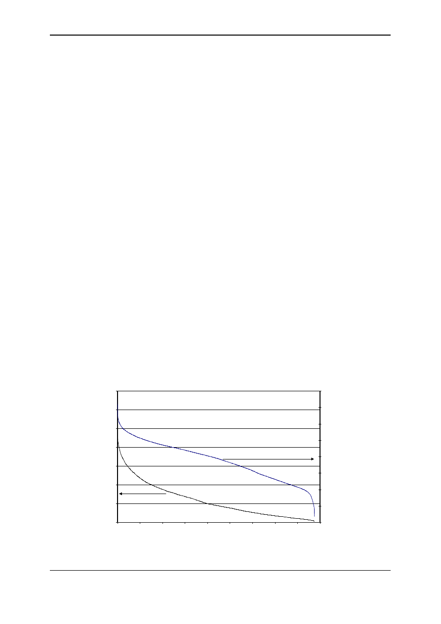
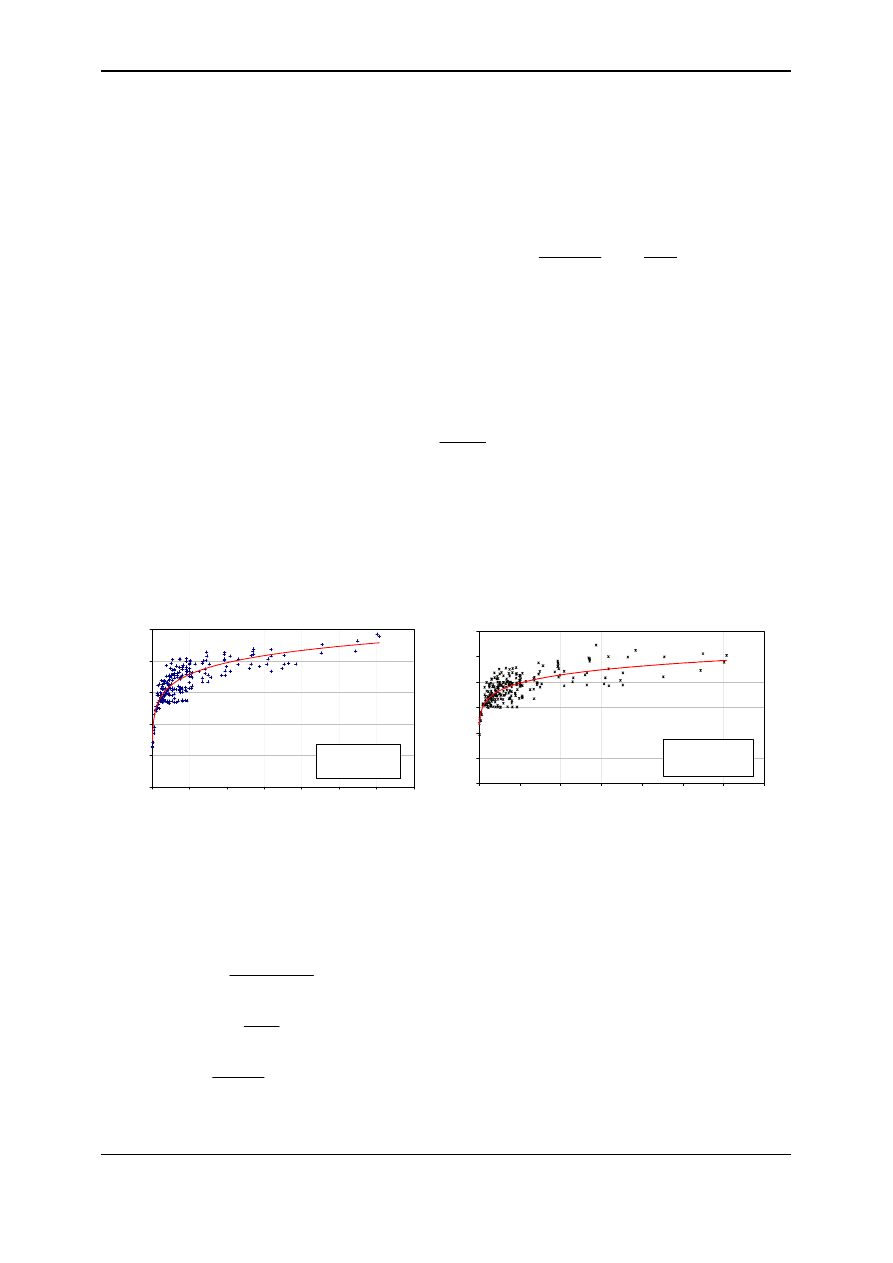
form of energy, the load duration curves can be used. The example of heat and electricity load
duration curves is shown in figure 2. The specific way of presenting the energy consumption
information is that the real loads are sorted from the maximum to the minimum one with no
matter when the specific load occurred.

0

200

400

600

800

1000

1200

1400

0

1000

2000

3000

4000

5000

6000

7000

8000

9000

Time

Heat

load, kW

0.00

20.00

40.00

60.00

80.00

100.00

120.00

140.00

160.00

Electric load, kW

Electricity

Heat

Fig. 2. Heat and electricity load duration curves of sample building

OPTI_Energy Centre of Excellence

www.itc.polsl.pl/centrum

68

Summer School: ENERGY SUPPLY FOR MODERN BUILDINGS, 21 - 24.09.2004, Gliwice, POLAND

The information provided by the load duration curve is as follows:
- maximum load,
- minimum load,
- average load,
- total amount of energy used,
- total annual time of energy demand,
- time t at which the energy demand

E

&

is higher than

.

)

(t

E

&

The load duration curves are typically used for:
- equipment sizing in separate energy supply systems,
- equipment sizing of cogeneration plants in the case when by products can be fully

disposed and there are no daily variations of energy prices,

- estimation of annual time of equipment operation,
- estimation of annual efficiency of equipment,
- definition of search range and trial solutions in optimization procedure.
The information that can not be read from the load duration curve is:
- real time of peak and valley demands,
- simultaneity of different types of loads.

Therefore, if built-in combined energy plant is planned the daily load profiles must be used. In
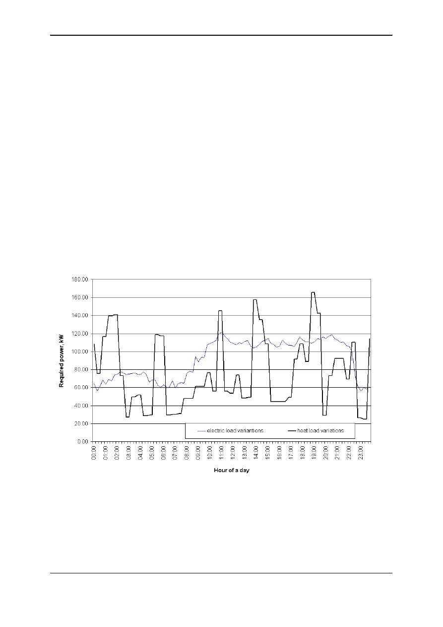
these curves the energy consumption data is presented as it occurs in time. The examples of
daily load duration curves is shown in figure 3.

Fig. 3. Example of daily load profiles at sample building

(measured at sport center with swimming pool)

The daily load profiles are typically used for:
- equipment sizing and optimization of cogeneration plants,
- simulations of machinery operation,
- estimation of part load operation time,
- variable load management,
- cost calculations.

OPTI_Energy Centre of Excellence
www.itc.polsl.pl/centrum

69

Summer School: ENERGY SUPPLY FOR MODERN BUILDINGS, 21 - 24.09.2004, Gliwice, POLAND

3.1. Building performance simulation

Most of buildings are not equipped with energy consumption monitoring systemsIn this

case the variations of loads can be analysed theoretically. In order to theoretically estimate the
energy demand variations at any building generally the dynamic model has to be applied. The
dynamic models can be divided into deterministic models and statistical models.
Deterministic models require detailed information about the physical system i.e. shape of the
building, construction, materials, configuration of rooms, installations, weather conditions and
many other parameters. On the other hand statistical models require an experimental data so
this type of analysis is limited mainly to the existing buildings.

In the case of electric loads the theoretical modeling is a very complicated task. The total

electric load of building can be divided into several components:

- lighting,
- lifts, automatic doors, alarms and monitoring systems,
- computers, copiers, projectors, TV sets, radios and other electric appliances,
- refrigerators, cookers, washers, driers, laundry and other utility equipment,
- water supply and sewage disposal equipment,
- ventilation and air conditioning equipment,
- heating and cooling systems.

Generally all the presented components can be divided into two main groups:

- human activity related,
- heating or cooling load related.
The first group of electric loads is very difficult to model theoretically, mainly because of

random components. The loads related to heating or cooling can be usually calculated from
energy characteristics of heating, cooling and air conditioning devices. On the other hand the
models of consumption of heat and cold have to be worked out first.

The total electric load of a building is always a sum of all partial electric loads that can be

classified into both of presented groups. Therefore the two following approaches are applied
usually:

- measurement and monitoring techniques are used at existing buildings,
- basing on a statistical data the typical models of load shapes are being worked out for

different types of buildings.

In the case of heat load profiles the modeling procedures lead to a more precise estimation

of the load variations. This is because the theoretical models of heat transfer process are able
to describe the real thermal conditions in a building with a better accuracy. It is also important
that there is relatively (comparing to electric loads) high thermal inertia of a building so the
thermal loads are not likely to change rapidly.

If a new building is just being designed the following types of deterministic models are

usually used:
- simplified steady state models – low accuracy, good for rough estimation of energy

demand at the extreme weather conditions,

- complex dynamic models – good accuracy, require time consuming modeling of a

building and significant time for calculations,

- complex dynamic models integrated with CFD (Computational Fluid Dynamics)

algorithms – give the best results, require the biggest processing capacity of computers and
the most detailed set of data including indoor climate conditions, temperature field, air
velocities, concentration of pollutants and other parameters.

In the case of existing buildings both measurements and statistical analysis (typically a

“black box” analysis) as well as theoretical modeling can be applied.

OPTI_Energy Centre of Excellence

www.itc.polsl.pl/centrum

70

Summer School: ENERGY SUPPLY FOR MODERN BUILDINGS, 21 - 24.09.2004, Gliwice, POLAND

In all cases the modeling procedure must lead to results that let us properly size the

building heating and cooling systems. Generally there can be couple of different heating or
cooling systems installed at the building. All this systems usually produce hot or cold water
that is subsequently led to building internal installations. Thus the particular output (system
load) can be calculated according to the formula:

)

(

in

out

w

w

S

T

T

c

G

Q

−

= &

&

(1)

where:

- system water flow,

- thermal capacity of water, T

- water output and

input temperature.

w

G

&

w

c

in

out

T

,

In order to size the heating and cooling system the model must predict all heat gains and

losses at the building. This is a common approach that in the modeling procedure a building is
divided into separate zones. Each zone is a finite volume element that can be in contact with
other zones, boundary surfaces or ambient environment. Within the each zone the following
phenomena can occur:

- convective heat transfer to/from boundary surfaces,
- radiative heat transfer between surfaces,
- radiative heat transfer to/from ambient environment
- heat and mass transfer to neighbouring zones,
- heat and mass transfer to/from ambient environment,
- heat and mass accumulation inside the zone.
There are number of differences between particular zones. The main ones are as follows:
- volume of internal air,
- number and types of other zones being in contact,
- internal temperature,
- function in the building,
- number of occupants,
- number and types of internal installations,
- number and types of equipment and appliances installed within a zone,
- number, size and thermal properties of internal mass inside a zone (different thermal

inertia),

For each zone a general energy balance can be written as follows:

w

d

E

d

dE

E

&

&

+

=

τ

(2)

Under transient conditions during exploitation of the building the energy demand

variations depend on such parameters like:
-

energy accumulation capacity of building (walls and internal air) and its internal

equipment,

-

thermal inertia of building

-

thermal inertia of internal installations,

-

thermal inertia of heat and cold sources,

-

control system (manual, automatic, mixed),

-

electric loads,

-

other.

Assuming that there is a constant amount of air inside the zone (input and output mass

flows are equal) and the air can be considered as an ideal gas the eq. (2) of the zone air energy
balance can be written as follows:

∑

∑

∑

∑

=

=

=

=

+

−

+

−

+

−

+

=

n

k

j

i

N

n

Sn

z

a

p

a

N

k

z

zk

p

k

N

j

z

j

j

j

N

i

i

z

v

Q

T

T

c

m

T

T

c

m

T

T

A

Q

d

dT

mc

1

1

1

1

)

(

)

(

)

(

&

&

&

&

α

τ

(3)

OPTI_Energy Centre of Excellence
www.itc.polsl.pl/centrum

71

Summer School: ENERGY SUPPLY FOR MODERN BUILDINGS, 21 - 24.09.2004, Gliwice, POLAND

where:

τ

d

dT

mc

z

v

- energy of an air inside the zone

∑

=

i

N

i

i

Q

1

&

- convective internal loads; N

i

– number of loads

∑

=

−

j

N

j

z

j

j

j

T

T

A

1

)

(

α

- convective heat transfer from surrounding surfaces, N

j

– number of

surfaces, T

j

– temperature of surface j, T

z

– zone air temperature

∑

=

−

k

N

k

z

zk

p

k

T

T

c

m

1

)

(

&

- interzone air flows, N

k

number of zones being in contact with analysed

zone,

)

(

z

a

p

a

T

T

c

m

−

&

- infiltration of ambient air, T

a

– temperature of ambient air,

∑

=

n

N

n

Sn

Q

1

&

- heating or cooling system load, N

n

– number loads

Additionally the surface energy balance must be taken into account as the internal air is

also heated or cooled by contact with surrounding surfaces. The energy balance equation of
surface j can be written as follows:

(4)

∑

=

−

−

+

−

=

+

j

N

l

l

j

l

j

z

j

j

ir

it

T

T

T

T

q

q

1

4

4

)

(

)

(

σ

ε

α

&

&

where:

it

q&

- heat transferred from (to) the surface to (from) a wall or other mass,

ir

q&

- sum of radiative heat fluxes from internal and external (solar) sources,

l

j

−

ε

- emissivity form wall j towards wall l (

l

j

≠ ),

c

σ

- Stefan-Boltzmann coefficient,

T

l

- temperature of wall

l,

Walls surrounding a volumetric zone as well as solid or liquid bodies inside the zone are

so called thermal masses. These masses are responsible for the thermal inertia of the building
being simulated. It can be introduced into the mathematical model of the building with using
the equation:

τ

ρ

d

dT

c

V

q

m

N

m

m

it

m

=

∑

=1

_

&

(5)

where: N

m

– number of heat transfer surfaces of the thermal mass

Equations (3), (4) and (5) are given in general form in order to present a complexity of the

modeling process. Solving the whole set of mathematical model equations requires advanced
numerical techniques to be used as well as proper computation capacity. There are also many
assumptions and simplifications to be made in order to complete the task. The most complex
and complicated procedures relate to:

- estimation of radiative heat transfer,
- estimation of convective heat transfer coefficients

α

j

,

OPTI_Energy Centre of Excellence

www.itc.polsl.pl/centrum

72

The modeling of a heat load variations is typically a sequential process where an

information from previous time step is used to calculate the system output and to update the
internal zone temperature at the current time. Time steps of one hour are typically used. On
the other hand the dynamic processes in the zone can occur on a much shorter time scale than

Summer School: ENERGY SUPPLY FOR MODERN BUILDINGS, 21 - 24.09.2004, Gliwice, POLAND

one hour. Some modern programs are able to run calculation with less then an hour time step
as well as with flexible, adaptive time step [9].

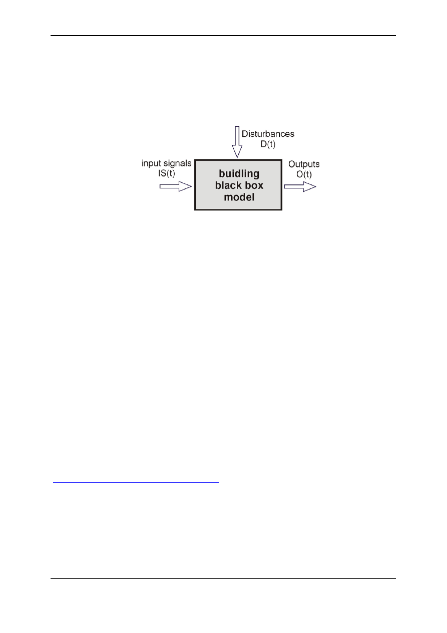
The complex real system does not allow for an easy and immediate physical justification

of a simulation parameters. In the case of existing building the stochastic modeling or so
called the “black box” model must be sometimes applied alternatively. A general approach to
a “black box” modeling philosophy is presented in fig. 4.

Fig. 4. Stochastic modeling of a building performance [1]

The model is supposed to produce an output values of defined variables if a particular

values of an input variables and disturbances are known. The disturbances include many
input-independent signals. In order to use this procedure the mathematical model of the
building must be identified first. The modeling is usually based on a set of polynomials. The
identification procedure means the selection of the final form of polynomials that have been
initially proposed in a general form. Modeling a building performance with using this
procedure requires a large set of historical data that can be used to “teach” the model.
Therefore this approach is mainly limited to existing buildings. If however the construction
parameters are used as the input data, the model can be worked out for a group of similar
buildings. A good example of using a “black box” philosophy is given in [1].

The simulation of building dynamic performance requires the detailed weather data [3].

The full set of weather data typically used in advanced building simulation software includes
hour to hour (or even more detailed) information about: dry bulb temperature, dew point
temperature, relative humidity, atmospheric station pressure, extraterrestrial horizontal
radiation, extraterrestrial direct normal radiation, horizontal infrared radiation from sky,
global horizontal radiation, direct normal radiation, diffuse horizontal radiation, global
horizontal illuminance, direct normal illuminance, diffuse horizontal illuminance, zenith
luminance, wind direction, wind speed, total sky cover, opaque sky cover, visibility, ceiling
height, present weather observation, precipitable water, aerosol optical depth, snow depth,
days since last snowfall. Obtaining such detailed set of data is itself a very complicated and
time consuming task.

There are many ready to use tools for simulations buildings and analysis of energy

demand variations. Some of the interesting computer packages can be found at:

http://www.eren.doe.gov/buildings/tools_directory/.

3.2. Predefined models of energy load variations

The detailed mathematical modelling of a building requires a lot of efforts, time and proper

computing capacity. On the other hand it was found in many studies that the objects of similar
functional types have also similar energy load variation characteristics [2][5]. Therefore in
many cases, if the results are expected in a relatively short time it is recommended to use
typical simplified predefined models instead of detailed energy consumption modelling of a
building.

OPTI_Energy Centre of Excellence
www.itc.polsl.pl/centrum

73

Summer School: ENERGY SUPPLY FOR MODERN BUILDINGS, 21 - 24.09.2004, Gliwice, POLAND

The predefined load shape curves are typically being worked out for groups of similar

objects. The curves usually cover representative days of an analysed period. The accuracy of
the estimation of energy consumption variations is higher if more typical periods are taken
into account. Typically the models of daily profiles of energy consumption are elaborated for
different type of days (weekdays, weekends, holidays etc.) and different seasons of a year
(summer, winter, midseason). The example of the heat load profile model is shown in fig. 5.

Models are typically given in a dimensionless form. The dimensionless consumption of

energy at time interval

∆τ is calculated for each selected type of day with using the following

formula:

∫

∫

=

h

d

E

d

E

E

24

0

2

1

2

1

τ

τ

τ

τ

τ
τ

&

&

(6)

In the similar way monthly and weekly energy consumption profile can be estimated.

Using the model presented in figure 5 requires only single parameter to be known. This

parameter is an annual heat consumption of the building. The value can be easily estimated
with using annual heat load duration curve and than it is decomposed into smaller portions
assigned to particular intervals of total annual time.

0

2

4

6

8

10

12

14

16

1

2

3

4

5

6

7

8

9

10

11

12

Month

Share of total annual heat consumption, %

0

2

4

6

8

10

12

14

16

18

20

1

2

3

4

5

6

7

Day of week

Share of total weekly heat consumption,

%

0,000

0,010

0,020

0,030

0,040

0,050

0,060

0,070

0,080

01:

00

02:

00

03:

00

04:

00

05:

00

06:

00

07:

00

08:

00

09:

00

10:

00

11:

00

12:

00

13:

00

14:

00

15:

00

16:

00

17:

00

18:

00

19:

00

20:

00

21:

00

22:

00

23:

00

00:

00

Hour of day

S

ha

re

o

f to

ta

l d

ai

ly

co

ns

um

pt

io

n, %

Fig. 5. Non-dimensional model of heating load variation elaborated for a group of specific

objects – schools with gym [5]

4. Systems of energy supply

OPTI_Energy Centre of Excellence

www.itc.polsl.pl/centrum

74

The most simple building energy supply system consists of energy delivery from external

utilities i.e. electric mains and heating networks. Nowadays there are many alternatives to this
solution. There are different technologies available in the market that make possible an on-site

Summer School: ENERGY SUPPLY FOR MODERN BUILDINGS, 21 - 24.09.2004, Gliwice, POLAND

generation of all required energy carriers at relatively low cost. The most popular
technologies are as follows:
a)

boilers,

b)

heat pumps,

c)

combined heat and power (CHP) modules based on:

- gas engines,
- microturbines,
- fuel cells,
- Stirling engines,

d)

fotovoltaic cells,

e)

solar collectors,

f)

compression and absorption chillers,

g)

hot or cold water accumulators.

Sophisticated systems of building energy supply typically make use of an integrated

solutions of more than one available technology. Additionally the built-in energy generation
system can co-operate with external utilities. The best technical and economic results can be
obtained if the system is configured and sized optimally under defined energy demand
variations and other technical and economic constraints. The examples of modern energy
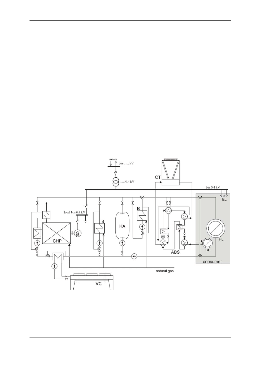
plants for building applications are shown in fig. 6 and 7.

Fig. 6. Building energy plant (CHP – cogeneration module with gas engine, VC – ventilator

cooler, B – gas boiler, HA – heat accumulator, ABS – absorption chiller, CT – cooling tower,

EL – electric load, HL – heating load, CL – cooling load)

OPTI_Energy Centre of Excellence
www.itc.polsl.pl/centrum

75

Summer School: ENERGY SUPPLY FOR MODERN BUILDINGS, 21 - 24.09.2004, Gliwice, POLAND

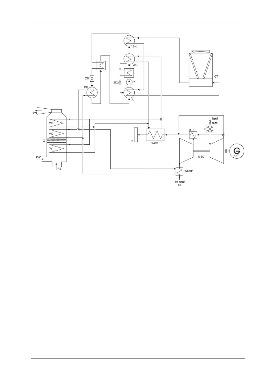
Fig. 7. Building energy plant with mictroturbine, absorption chiller and conditioning plant

(MTG – microturbine, WCHP – air coolin heat exchanger, WKO – heat recovery boiler, R –

recuperator, K – chimney, W1, W2, W3 – heat exchangers, Z – water trap, PS – stream of

fresh air, PW – stream of recirculation air, PN – air to the building, A – absorber, P – pump,

ZD1, ZD2 – throttle valves, PR – evaporator, WR – generator, SK – condenser, CT – cooling

tower)

5. Modelling and optimization of energy plants

The modern building energy supply system design process requires the following

guidelines to be taken into account:
-

final technical solution should result from maximization of an economic effect,

-

plant configuration and energy production capacity should be optimized,

-

energy production machinery and devices usually can operate only within allowable

range of loads (thermal or electric),

-

different units have different energy efficiency characteristics,

-

it is difficult to produce exactly as much energy as is required by the building; there

will be usually either surpluses or shortages,

-

first and second law of thermodynamics are always valid.

OPTI_Energy Centre of Excellence

www.itc.polsl.pl/centrum

76

The building energy supply system design procedure is usually decomposed into two

separate tasks including demand side analysis and supply side analysis. These two subtasks
are being integrated by the system load variation curves. It must be however taken into
account that the operation of energy supply system may have an impact on an energy demand
of a building. Therefore, if it is possible the whole task is being solved in iterative loop. The
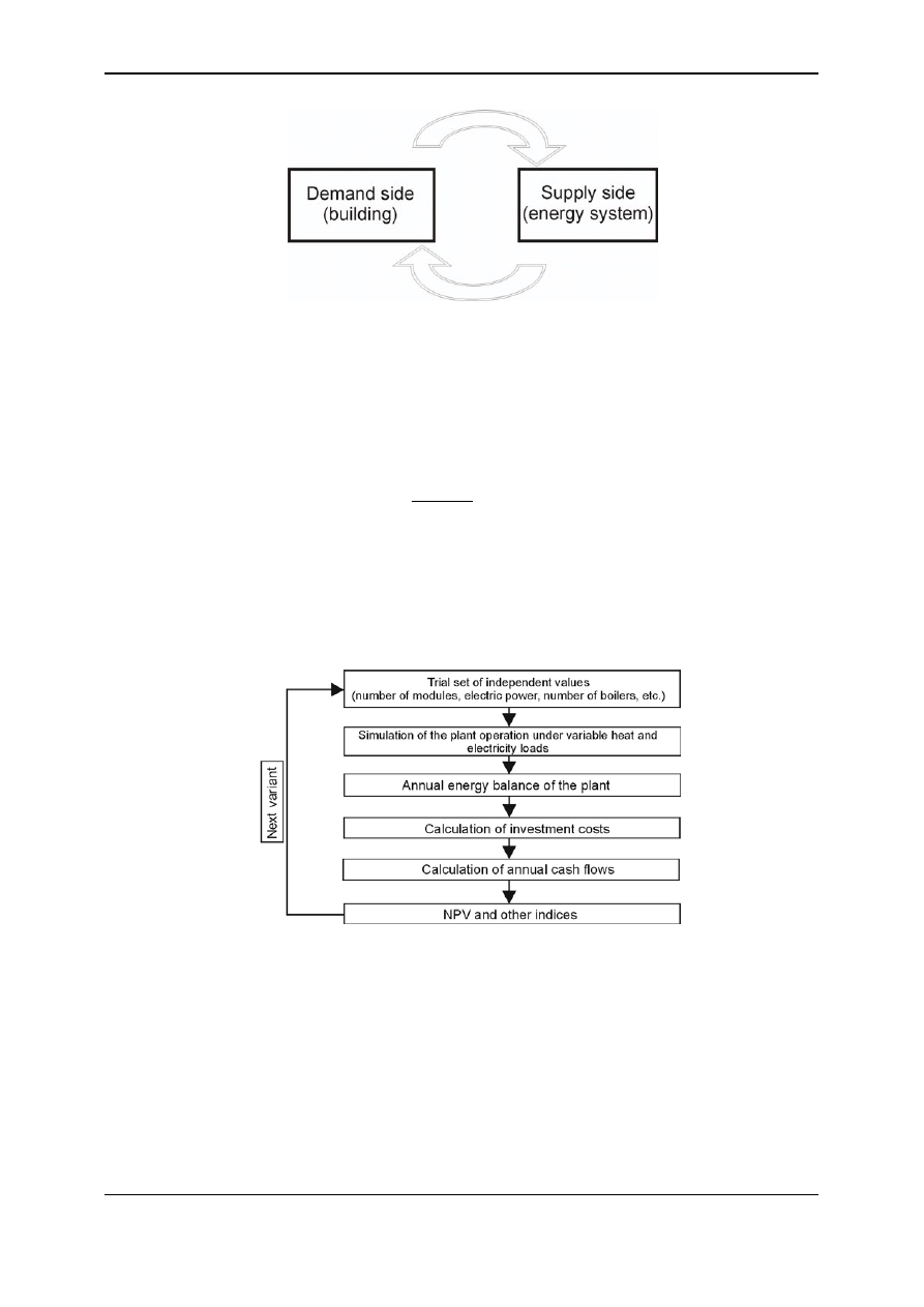
schematic diagram is shown in fig. 8.

Summer School: ENERGY SUPPLY FOR MODERN BUILDINGS, 21 - 24.09.2004, Gliwice, POLAND

Fig. 8. Integration of modelling procedures

The methodology for modelling and optimization of a building energy plant is shown on

the example of a built-in small scale cogeneration plant. General energy demand
characteristics of building is shown in the form of load duration curves in fig. 2. The analysis
is performed hour by hour with using daily heat and electricty load profiles.

The objective function for the plant optimisation procedure is the Net Present Value of the

project for specific time of economic life (typically N = 15 years) [7]:

∑

=

→

−

+

=

N

t

t

t

J

r

1

0

max

)

1

(

CF

NPV

(7)

where:

CF

t

– annual cash flow in year

t, r – discounted cash flow rate, J

0

– initial investment

capital.

The objective function is typically constrained by technical parameters of the plant and the

economic environment. Therefore the complete analysis consists of two integral parts:
technical analysis and economic analysis. Scheme of the optimization algorithm is shown in
fig. 9.

Fig. 9. Block diagram of plant sizing optimisation procedure

The plant being analysed is similar to that presented in fig. 6 with the only difference that

there is no absorption chiller installed. The momentary energy balance for the entire CHP
plant can be written as follows:

(8)

str

D

S

D

G

d

Q

Q

N

N

N

W

P

&

&

&

+

+

−

−

=

+

)

1

(

δ

δ

where:

– stream chemical energy of fuel,

N

d

W

P

&

G

– electricity from the grid,

δ

– binary

variable,

N

D

– building electricity demand (from load shape curve), N

S

– surplus electricity,

- building head demand (from load shape curve),

- heat loss.

D

Q

&

str

Q

&

Particular elements of the equation (8) can be decomposed as follows:

OPTI_Energy Centre of Excellence
www.itc.polsl.pl/centrum

77

Summer School: ENERGY SUPPLY FOR MODERN BUILDINGS, 21 - 24.09.2004, Gliwice, POLAND

(9)

∑

∑

=

=

−

−

+

+

=

P

CHP

n

k

Pj

S

G

n

i

CHPi

D

N

N

N

N

N

1

1

)

1

(

δ

δ

(10)

Q

Q

Q

Q

Q

Q

A

str

n

j

Kj

n

i

CHPi

D

K

CHP

&

&

&

&

&

&

∆

+

+

−

+

=

∑

∑

=

=

1

1

∑

∑

∑

∑

=

=

=

=

+

=

+

=

CHP

K

CHP

K

n

i

n

j

Ekj

Kj

CHPi

E

CHPi

n

i

n

j

Kj

d

CHPi

d

d

Q

N

W

P

W

P

W

P

1

1

_

1

1

)

(

)

(

η

η

&

&

&

&

(11)

where:

N

CHPi

– electric power of CHP module i, N

Pj

– electricity consumption by plant device

j,

- heat output of CHP module

i,

- heat output of boiler

j,

- heat from

accumulator (

>0 – accumulator unloading,

<0 – accumulator loading),

- heat

shortage,

η

CHPi

Q

&

Kj

Q

&

A

Q

&

A

Q

&

A

Q

&

Q

&

∆

E

– energy efficiency

Ratio of electricity and heat for CHP plant is expressed by the cogeneration index

σ:

CHPi

CHPi

i

Q

N

&

=

σ

(12)

The minimum value of the cogeneration index

σ is limited by the maximal possible heat

output of the particular gas engine.

Particular parameters of the machinery characteristics (

η

E_CHP

,

σ

)

typically depends on the

nominal electric power and momentary load. Figure 10 presents the energy characteristics of
cogeneration modules with gas engines worked out for the purpose of preliminary machinery
sizing procedure.
a)

b)

η = 23,485 N

0,0691

R

2

= 0,7203

20

25

30

35

40

45

0

1000

2000

3000

4000

5000

6000

7000

moc elektryczna, kW

s

p

ra

wnoś

ć

η

, %

σ = 0.3605 N

0.1137

R

2

= 0.5821

0

0,2

0,4

0,6

0,8

1

1,2

0

1000

2000

3000

4000

5000

6000

7000

moc elektryczna, kW

wskaźnik skojarzenia

σ

Fig. 10. Efficiency (a) and cogeneration index (b) of gas engine based CHP modules in the

electric power range of 50 – 6000 kW (note: exhaust gases cooled down to 120

O

C)

In order to estimate heat output and fuel energy consumption at partial loads the following

dimensionless characteristics of the CHP module have been used:

( )

( )

( )

6537

.

0

587

.

0

2431

.

0

0025

.

0

)

(

2

3

_

_

+

+

−

=

el

el

el

nom

CHP

E

CHP

E

ξ

ξ

ξ

η

η

(13)

( )

( )

( )

3968

.

0

7756

.

1

9848

.

1

8147

.

0

2

3

+

+

−

=

el

el

el

nom

ξ

ξ

ξ

σ

σ

(14)

where:

- dimensionless load,

el

ξ

= 0.2 – 1.

nom

el

el

el

N

N

_

=

ξ

Efficiency of gas boilers is mainly a function of heat transfer area. Therefore for each

nominal heat output of the boiler the same value of efficiency can be reached. It was assumed

OPTI_Energy Centre of Excellence

www.itc.polsl.pl/centrum

78

Summer School: ENERGY SUPPLY FOR MODERN BUILDINGS, 21 - 24.09.2004, Gliwice, POLAND

that this values is fixed at the level

η

Ek

= 0.92 and it does not vary with the nominal heating

power of the boiler. In order to estimate the behaviour of the boiler at partial loads the
following dimensionless characteristics has been used:

( )

9556

.

0

1165

.

0

1096

.

0

1693

.

0

1318

.

0

2

3

4

−

+

−

+

−

=

x

x

x

x

nom

Ek

Ek

η

η

(15)

where:

nom

Q

Q

x

&

&

=

- dimensionless load.

It was found from the heat load duration curve that the maximum heat demand occurs only

during a very short period of time over the year. Therefore it is needless to size the heating
system for maximum load as it will mostly operate at partial load (with lower efficiency). It is
usually possible that the building designer allows shortages of heat in some periods. This
allowances must be known at the stage of planning the heating system. The temporary heat
shortages

can be included in energy balance of the plant:

Q&

∆

(16)

D

Q

Q

&

&

α

=

∆

The

α index must be controlled over all period of the simulation of plant operation. If the

value of the index or the time of its appearance exceed the set up limits the system must be
configured again.

Each machine or device can operate only within the defined range of allowable load. It

means that the following inequality constraints have to be taken into account:

(

)

(

)

nom

CHPi

CHPi

CHPi

N

N

N

≤

≤

min

17)

( )

( )

nom

Kj

Kj

Kj

Q

Q

Q

&

&

&

≤

≤

min

(18)

If the local cogeneration system has to meet simultaneous demands for heat and electricity

there can be defined the total number of 9 cases of relations between the heat and electricity
demands and the production capacities of the plant. It was found that the priority of the
system operation strongly influences the final economic effect of the project [7]. There are
several possible modes of CHP module operation. In this paper the following modes are taken
into account:
1) electricity tracking (ET) – in this mode the priority is electricity production. The power of

the cogeneration module is following the demand of the consumer. There is no transfer of
surplus electricity to the external utility grid. Heat demand is balanced by the boiler or
heat storage tank. If there is a surplus heat it is dissipated into the atmosphere.

2) heat tracking (HT) – in this mode the priority is heat production. The heat output of the

cogeneration module is following the demand of the consumer. CHP module usually
operates in parallel with boilers. Electricity demand is balanced by the grid.

3) full load operation (FL)– cogeneration module is run at full load no matter what the

demand of the consumer is. The momentary energy balance of the plant converges by the
cooperation with grid, boilers, storage tanks, ventilator coolers and other devices.

Almost each cogeneration module equipped with standard automatic control system can

run in the above defined modes.

Optimization of the plant was done by searching for the best solution within the predefined

range of trial variants. Energy balance calculations were performed as an “hour by hour”
simulation of the plant operation. The analysis was carried out with using an Excel
spreadsheet and Visual Basic macros. Columns of the spreadsheet (matrix) represent
particular positions of equations (2) – (5), whereas the rows represent time. Once the annual
energy balance of the plant is done the economic analysis starts.

OPTI_Energy Centre of Excellence
www.itc.polsl.pl/centrum

79

Summer School: ENERGY SUPPLY FOR MODERN BUILDINGS, 21 - 24.09.2004, Gliwice, POLAND

The economic analysis basis on the cash flow CF calculation for the whole lifetime of the

project:

(19)

(

)

∑

∑

=

=

+

−

+

+

−

+

−

=

=

N

t

t

d

R

op

E

n

N

t

t

L

P

S

K

K

S

J

CF

0

0

0

)

(

CF

where:

S

n

– cash incomes (=0),

K

E

– cost of exploitation,

K

op

– other operational costs,

P

d

–

income tax,

L – loses, t – number of year.

In order to estimate investment costs

J

0

the typical curves of unitary cost

i were used:

a) for gas boilers (boiler purchase cost, zł/kW):

(20)

13

.

0

250

−

=

nom

Q

i

&

where

Q

denotes nominal heat output in kW. Heat output range 50 kW to 10000 kW.

nom

&

b) cogeneration module with gas engine (together with ventilator cooler) – unitary cost in
US$/kW within the electric power range 9 kW do 6000 kW:

(21)

2857

.

0

)

(

9

.

2594

−

=

nom

N

i

All additional costs were estimated either with using a typical cost breakdown or the offers

from vendors. It appeared that equipment purchase cost lays down typically in the range of
40% to 60% of the total investment cost

J

0

.

In our case real incomes appear only for HT or FL modes of cogeneration module

operation. The income results from the sale of the electricity surplus to the grid and it is
calculated as follows:

(22)

∫

=

R

d

N

S

S

n

τ

τ

0

Total exploitation cost can be expressed as follows:

env

p

M

O

en

E

K

K

K

K

K

+

+

+

=

&

(23)

where: K

en

– costs of energy, K

O&M

– operation and maintenance costs, K

p

– personal costs,

K

env

– environmental costs.

The most important is the cost of energy:

τ

τ

η

η

τ

τ

τ

d

k

N

k

LHV

Q

k

LHV

N

d

K

K

R

K

CHP

R

el

G

n

j

fk

Ekj

k

Kj

n

i

fCHP

CHPi

E

CHP

CHPi

en

en

∫

∑

∑

∫















+

+

=

=

=

=

0

1

1

_

0

)

(

&

&

(24)

Operating and maintenance costs were calculated with using the typical index of unitary

costs for gas engines

k

O&M

= 0.007 do 0.02 US$/kWh (at annual availability in the range of

92 – 97 %). Therefore the following equation can be used:

(25)

∫ ∑

=

=

=

R CHP

d

N

k

k

E

K

n

i

CHPi

M

O

M

O

el

M

O

τ

τ

0

1

&

&

&

Environmental costs are given by equation:

(26)

(

)

[

]

τ

τ

τ

τ

τ

τ

d

k

G

d

k

G

G

d

K

K

R

R

R

W

W

n

i

Pi

k

Pi

CHP

Pi

env

env

∫

∑ ∫

∫

+

+

=

=

=

0

1 0

_

_

0

&

&

&

&

Typically

are calculated with using emission indices for particulate

machinery type. Emission fees in Poland are regulated by the government: SO

B

P

CHP

Pi

G

G

_

_

,

&

&

2

- 0.38

PLN/kg; CO

2

- 0.00020 PLN/kg; CH

4

- 0.00020 PLN/kg; NO

2

- 0.38 PLN/kg; CO - 0.10

PLN/kg; NMHC - 0.10 PLN/kg; dust - 0,25 PLN/kg (Note: 4.7 zł = 1 EURO).

OPTI_Energy Centre of Excellence

www.itc.polsl.pl/centrum

80

Summer School: ENERGY SUPPLY FOR MODERN BUILDINGS, 21 - 24.09.2004, Gliwice, POLAND

6. Results of sample analysis

In the reference case of calculations it has been assumed that no cogeneration module will

be installed on site. The existing coal fired boiler plant will be replaced with gas boiler plant,
electricity will be purchased from the utility grid separately for each building. Proposed gas
boiler plant would consist of three gas boiler of respectively 350, 350 and 200 kW heat
output. Fuel and energy prices, that were used in the analysis, are as follows:

• Natural gas price depends on an annual consumption,

average value is: 0.796 PLN/Nm

3

.

• Electricity price: - sport centre (tariff C21): 328.67 PLN/MWh,
- school (tariff C11): 336,17 PLN/MWh.

Technical and economic results of the project are given in table 1.

Table 1

Results of technical and economic analysis for base case project

No. Quantity

Unit

Value

1 Amount of heat produced at boiler plant

GJ/a

7272

2 Heat shortage

GJ/a

54

3 Total amount of electricity from utility grid

kWh/a

661 637

4 Total amount of natural gas burned

Nm

3

/a

230 871

5 Average efficiency of the boiler plant

%

90.7

6 Total cost of electricity

PLN/a

218 600

7 Total cost of natural gas

PLN/a

183 750

8 Investment cost

PLN

466 540

9 Net Present Value after 15 years

PLN

-3 463 600

PLANT WITH COGENERATION MODULE

Table 2 presents the configurations of the cogeneration plant that were defined as trial

solutions for optimization procedure.

Table 2

Selected variants of the configuration of the plant

Number of variant

Nominal parameter

1

2

3

4

5

6

7

8

9

10

11

N

CHP

kW

20 30 40 50 60 70 80 90 100 110 120

kW

44 62 79 96 112 128 143 158 173 188 203

kW

350 350 350 350 350 350 350 350 330 300 300

kW

350 350 300 300 300 285 275 260 260 260 250

kW

160 140 170 155 140 140 140 140 140 150 150

1

K

Q&

CHP

Q&

2

K

Q&

3

K

Q&

It was assumed that there will be only one cogeneration module. The minimal allowable

electric load of the module was set in the value of 40% of nominal power. Figures 11 and 12
show the results of technical analysis. In the electricity tracking mode there is no sale of the
electricity surplus electricity to the grid, however if the installed electric power of the CHP
module is higher, the production is much lower than potentially possible (compare to FL
mode). On the other hand in the ET mode the loss of heat form CHP module is lower.

OPTI_Energy Centre of Excellence
www.itc.polsl.pl/centrum

81

Summer School: ENERGY SUPPLY FOR MODERN BUILDINGS, 21 - 24.09.2004, Gliwice, POLAND

0

100

200

300

400

500

600

700

800

900

1000

1100

20

30

40

50

60

70

80

90

100

110

120

MWh

Nominal electric power of the CHP module

Gross electricity production - ET mode
Gross electricity production -HT mode
Gross electricity production - FL mode
Electricty sold to the utility grid in HT mode
Electricty sold to the utility grid in FL mode

0

100

200

300

400

500

600

700

800

900

1000

1100

1200

1300

1400

1500

1600

1

2

3

4

5

6

7

8

9

10

11

Nominal electric power of the CHP module

Heat

loss, GJ/a

Heat loss in ET mode

Heat loss in FL mode

Fig. 11. On-site electricity production and heat loss in particular variants of the plant

configuration

0,75

0,80

0,85

0,90

0,95

20

30

40

50

60

70

80

90

100

110

120

Nominal electric power of the CHP module

Total efficiency of

the C

H

P

m

odule

ET mode
HT mode
FL mode

0,75

0,80

0,85

0,90

0,95

20

30

40

50

60

70

80

90

100

110

120

Nominal electric power of the CHP module

Net

total

e

ffi

ci

ency

of

the

p

la

nt

ET mode
HT mode
FL mode

Fig. 12. Total efficiency (EUF) of the cogeneration module and the whole plant

In the HT and FL modes of CHP module operation the electricity can be sold to the mains.

If so, the selling price of surplus electricity will be 140

PLN/MWh.

Figure 13 shows the results of the economic analysis in relation to the reference case. It

was found that the best mode of operation of the CHP module is electricity tracking. It was
also found that there is an optimal solution that consists in installation of CHP module in 80 –
90 kW electric power range and three gas boilers. The difference in NPV comparing to base
case analysis is at the level of investment cost.

0

50000

100000

150000

200000

250000

300000

350000

400000

450000

20

30

40

50

60

70

80

90

100

110

120

Electric power of the CHP module, kW

Dif

fe

rence in NPV in comparison t

o

ref

erence

case, PLN

Mode: Electricity tracking
Mode: Heat tracking
Mode: Full power

Fig. 13. Results of the optimization procedure

7. Conclusions

The demand for heat and electricity at any object is never constant. If a building built-in

plant is considered to be installed at a local energy system, it is necessary to work out the

OPTI_Energy Centre of Excellence

www.itc.polsl.pl/centrum

82

Summer School: ENERGY SUPPLY FOR MODERN BUILDINGS, 21 - 24.09.2004, Gliwice, POLAND

daily load profiles for an each energy carrier required by the building. Only in this case it can
be estimated if all useful products of the plant can be fully utilized, what is the remaining
demand for electricity from the utility grid and for heat from boilers, in what hours the CHP
module can be switched on and off, if there is a need for heat storage tank and what the total
cost of energy supply will be, etc.

It was presented that the analysis of energy demand is a quite complicated and time

consuming task. The energy demand must be estimated in order to configure and size
machinery and devices of energy supply system.

It has been also presented that the optimal solution of energy supply system exists and it

can be initially identified by using a general model of the plant and statistical parameters of
machinery characteristics. The presented model is also suitable for selecting the optimal mode
of the cogeneration module operation.

8. References

[1] Bondi P., Cardinale N., Stefanizzi P.: A stochastic dynamic method for the evaluation of

the heating power input of a real building-plant system. Energy and Buildings. No 26
(1997)

[2] Corfitz Noren: Typical load shapes for six categories of Swedish commercial buildings.

Department of Heat and Power Engineering, Lund Institute of Technology. Lund,
Sweden. ISSN 0282-1990

[3] Crawley B.D., Hand W.J., Lawrie L.K.: Improving the weather information available to

simulation programs.

[4] Gilijamse W., Boonstra M.E.: Energy efficiency in new houses. Heat demand reduction

versus cogeneration. Energy and Buildings. No 23 (1995)

[5] Institut Wallon: Demande de Chaleur Techniquement Cogenerable Pour la Region

Wallonne Et la Region de Bruxelles Capitale. Raport final. Mai 1997, Namur, Belgium

[6] Kalema T., Haapala T.: Effect of interior heat transfer coefficients on thermal dynamics

and energy consumption. Energy and Buildings. No 22 (1995)

[7] Kalina J. Analysis and optimization of the small-scale combined heat and power

systems. PhD thesis. Silesian Technical University at Gliwice, Poland. Gliwice, 2001.

[8] Skorek J. Analysis of technical and economic effectiveness small-scale cogeneration

plants fuelled with gaseous fuels. Silesian University of Technology Publishing, Gliwice
2002. (in Polish) ISBN 83-7335-127-2

[9] US Department of Energy: Energy Plus Engineering Document. The Reference to

EnergyPlus Calculations. EnergyPlusTM, Version 1.1, April 2002

[10] Witzani M., Pechtl P. Modelling of (cogeneration)-power plants on time dependent

power demands of the consumer. Materiały konferencji ASME Cogen-Turbo
Conference. Wiedeń, Austria, August 1995.

[11] Zhai Z., Chen Q., Klems J.H., Haves P.: Strategies for coupling energy simulation and

computational fluid dynamics programs. VII International IBPSA Conference, Rio de
Janeiro, 2001.

Useful web resources:

http://www.eren.doe.gov/buildings/tools_directory/
http://www.strath.ac.uk/Departments/ESRU
http://www.eren.doe.gov/buildings/energy_tools/energyplus.htm

OPTI_Energy Centre of Excellence
www.itc.polsl.pl/centrum

83

Summer School: ENERGY SUPPLY FOR MODERN BUILDINGS, 21 - 24.09.2004, Gliwice, POLAND

OPTI_Energy Centre of Excellence

www.itc.polsl.pl/centrum

84