Pyramid Tracing vs. Ray Tracing for the simulation of sound
propagation in large rooms.

A. Farina
Department of Industrial Engineering, University of Parma,
Via delle Scienze, I-43100 PARMA, Italy

Abstract
The aim of this paper is to introduce a new computational model (RAMSETE)
for the simulation of sound propagation in large rooms; the model can easily be
adapted to work outdoor, and can consider diffraction effects around screen
edges and sound paths passing through (light) panels.

However, this paper focuses on room acoustics, and particularly on rooms

with non-Sabinian behaviour. In fact, the Pyramid Tracing algorithm does not
involve an hybrid computation scheme, with a reverberant tail superposed to
the deterministic early reflections estimate, as it is common with other
diverging beam tracers (cone tracers, gaussian beam tracers, etc.). This make it
possible to study also sound fields characterised by double-slope sound decays,
inside spaces with not comparable dimensions and inhomogeneous sound
absorption.

It is well known that the same capabilities were already present in the

(original) Ray Tracing scheme, but requiring much longer computation time. In
fact, a correct Ray Tracing implementation can be considered as the reference
standard for any (faster) numerical code based on the Geometrical Acoustics
assumptions.

After a brief introduction to some important details of the two algorithms,

the results obtained in three cases are presented. The first is a typical Sabinian
room (a reverberating chamber), the second is the coupling of two rooms with
different average absorption (a theatre with its stage), the third is a typical
industrial building (having an height very little compared to other dimensions)
with non-uniform sound absorption (baffles under the ceiling).

The results show how the Pyramid Tracing can give results very similar to

the original Ray Tracing, provided that a proper adjustment of the parameters is
performed. On the other hand, the magnitude of the errors that can be done
with improper parameter settings is delimited and discussed.
1. Introduction to the two algorithms

Before we can present the results of the comparison tests, it is better to explain
briefly the working principles of the two codes used here. Both of them run on
a standard PC, under MS-Windows, and share the same input and output file
formats, so the comparison is easy.

All the files are plain-ASCII, with auxiliary strings embedded to make easy

to understand the meaning of each row of data. The input data file is produced
by a dedicated 3D CAD program, and the output files are processed through a
set of graphical utilities capable of reconstructing, from the “raw” impulse
response data, the usual descriptors used in room acoustics: Levels, Early-to-
Late ratios, Lateral Efficiency, Center Time, STI, etc. . The only difference
during the post processing is that the impulse responses produced by the
pyramid tracing must be corrected prior of calculating such parameters, as
explained in another paper (Farina [1]).

1.1 The Ray Tracing program
The Ray Tracing program used here is the evolution of a computer code
initially developed from the author and Prof. Alessandro Cocchi (University of
Bologna, Italy) for the study of large, non-Sabinian spaces (Farina[2]). The
details of this code were never published before.

The original Ray Tracing scheme is assumed: a large number of non-

diverging rays is isotropically traced from the (point) source, bouncing
specularly over the room boundaries, where part of their energy is absorbed.
The receivers are spheres of proper radius, and the detection mechanism make
it possible to compute the Sound Energy Density (J/m

3

) inside the receiver

volume, as shown in fig. 1.

R

S

L

Figure 1 - Conceptual scheme of the Ray Tracing algorithm

The contribution W’ to the total energy density W that each ray leaves

inside the receiving sphere is proportional to the length of the intersection L
and to the initial energy reduced for multiple absorption on the boundary
surfaces (with absorption coefficients

α

i

) and for the air absorption (with

coefficient

γ

multiplied for the path length x):

(

)

[

]

W

P

Q

N

c V

L

e

wr

rays

sphere

i

i

x

'

=

⋅

⋅ ⋅

⋅ ⋅

−

⋅

∏

− ⋅

ϑ

γ

α

1

(1)

This formulation avoids the common inconsistencies present in other

detections schemes (as surface intensity over the sphere surface or over a
circular disk), that are not physically compatible both with free field and
reverberant spaces.

Another remarkable point is the ray generation at the source. Although the

Ray Tracing scheme requires a random generation, it must be ensured that the
generation is almost uniform on the surface of a spherical source (the source
directivity Q

θ

is managed along with the energy assigned to each ray, as shown

in eqn 1). The simple assumption of three random generators for the three
versor components of the ray is not correct, as this produce a “cube of rays”
instead of a sphere; it is possible to “cut away” the corners of the cube
(discarding each vector having modulus greater than 1), but it was preferred to
employ a semi-probabilistic generator, in which the sphere surface is
mathematically divided in a large number of equal areas (actually 400=20x20),
each of them being “brushed” with the random generators.

This task was accomplished employing just two random generators (RND1

and RND2), and projecting their values over the sphere to obtain the versor
components of the ray:

v

i

RND

i

RND

j RND

v

i

RND

i

RND

j RND

v

i

RND

i

j

x

y

z

= ⋅

+

− +









⋅

⋅ ⋅ +









= ⋅

+

− +









⋅

⋅ ⋅ +









= − ⋅ +

=

=

2

1

20

1

20

2

2

20

2

1

20

1

20

2

2

20

1 2

1

20

0 19

0 19

2

2

cos

sin

..

..

π

π

(2)

This is equivalent to cutting the sphere with 20 iso-z planes, equally

spaced along the z axis, and then dividing each circle again in 20 parts, as
shown in figure 2. Obviously this causes the single facets to have very different
shape, but all have the same area.

The generation is then repeated many times, until the wanted number of

rays (usually more than 100.000) is reached.

This Ray Tracing program has proven to be very accurate and reliable,

provided that a very high number of rays is generated. This is easily verified, as
the program can proceed indefinitely, increasing the number of rays (in packets
of 400) until a convergence criterion is satisfied (for example on the SPL in a
particular receiver, that must stabilise within a pre-defined tolerance).

A further validation of this Ray Tracing program has been obtained

through participating at the benchmark organised by Verbandt & Jonckheere
[3] in 1992: in that case this ray tracing code (labelled 8aS in that comparison)
resulted perfectly aligned with the other 7 (more famous) participants.

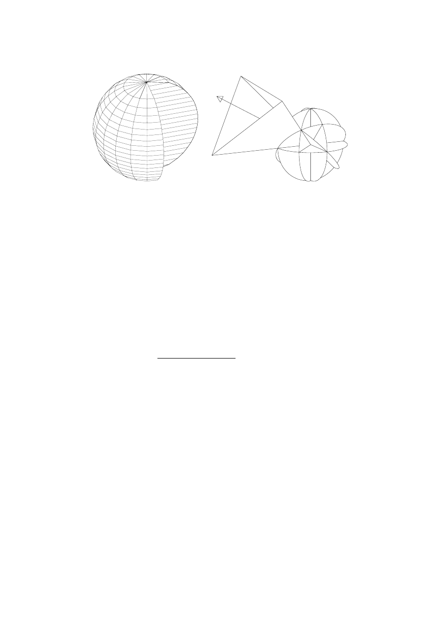
Figure 2 - subdivision of the source’s surface in facets of equal area (Ray

Tracing, left) and in triangular beams (Pyramid Tracing, right)

1.2 The Pyramid Tracing program
Ramsete is one of the first pyramid tracing codes that was developed for room
acoustic simulations. At the time of its first appearance (1993), only the work
of Lewers [4] reported a “triangular beam tracing” hybrid method.

In the Pyramid Tracing scheme, triangular beams are generated at the

sound source, as shown in fig. 2. The central axis of each pyramid is traced as
usual, being specularly reflected when it hits on a surface. The three corners of
the pyramid follow the axis, being reflected from the same plane where it hits.

The receivers are points, and a detection occurs when this point is inside

the pyramid being traced. In this case, a pseudo-intensity contribution I’ is
recorded (along with the time elapsed since pyramid emission) for each octave
band:

I

P

Q

x

e

wr

i

i

x

'

(

)

=

⋅

⋅

−

⋅ ⋅

⋅

∏

− ⋅

ϑ

γ

α

π

1

4

2

(3)

in which x is path length,

γ

is the absorption coefficient of air, Q

θ

is the

directivity factor and P

wr

is the acoustic power of the source.

Ramsete is not an hybrid model: the tracing of pyramids is prosecuted up

to the whole time length required to analyse the impulse response, and no point
of transition exist between the “early” part of the decay and the “late” one. The
author already published the details of the tail correction algorithm (Farina [1]).

For the purposes of the present work, it is necessary to recall here the

meaning of the two numerical parameters

α

and

β

, the value of which need to

be adjusted to model non-sabinian spaces with a little number of pyramids.

αααα

: is the exponent to be applied to the current time, to find the number of

reflected waves arriving to a receiver in the time unit (usually called temporal
echo density). For example, in Sabinian room

α

=2, in a tunnel-like room it

approaches 1, while in a very low room (only 2 counterpoised surfaces) the
temporal echo density is constant, so the exponent

α

is 0. in some cases

α

can

also be very greater than 2.

ββββ

: is a coefficient inserted in the formula for calculating the critical time

t

c

: this is defined as the time at which the “true” temporal echo density (that

usually increases with time) is equal to the “false” constant echo density
produced by the pyramid tracing (that is simply proportional to the number of
pyramids, and inversely proportional to the mean free path). The parameter

β

can adjust t

c

from infinity (no correction,

β

=0) to the Sabinian value

(

β

=0.3).(Farina[1])

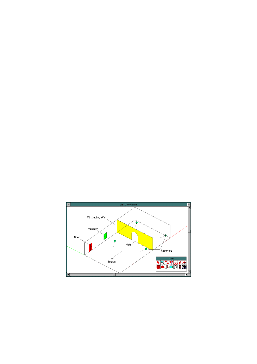
Another point that need to be explained here is the capability to treat

“holed” and “obstructing” surfaces, as this greatly speeds up the program.
Usual surfaces are quadrilateral plane faces, defined by the coordinates of their
vertexes. If they are declared “obstructing”, additional tests are made to find the
sound attenuation of pyramids “passing through” the panel and being diffracted
from its free edges (automatically located). On a surface it is also possible to
“attach” three types of entities: doors, windows and holes. Doors and windows
are rectangular areas, having absorption coefficients and sound reduction
indexes different from that of the wall. The holes are closed polylines, that
define regions where the pyramids can freely pass through an obstructing wall.

These features produce a noticeable reduction in computing time, as the

number of (main) surface is reduced, and the complete set of tests is conducted
on the “obstructing” surfaces only. Figure 3 show an example (from Ramsete
Cad) of these modelling capabilities.

Although Ramsete is not a Montecarlo method, still a convergence to the

“right” values can be seen increasing the number of pyramids traced: the goal
of this work is to find the right values of coefficients

α

and

β

, making it

possible to obtain correct results using just 256 pyramids or even less, with
computations times reduced to a couple of minutes for each sound source in the
worst cases.

Figure 3 - Advanced Surface Attributes in Ramsete

2. Comparison between the two algorithms

2.1 A Sabinian room
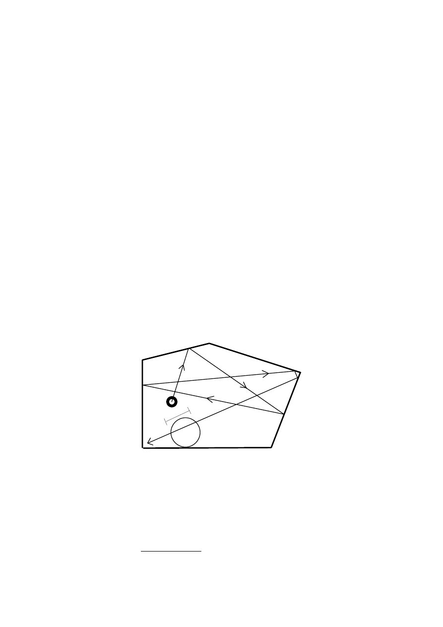
Figure 4 shows the geometry of a classic reverberant chamber:

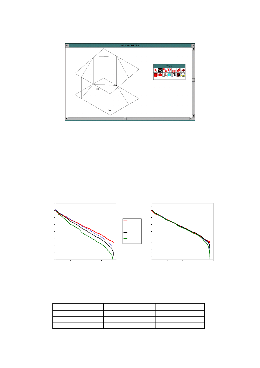
Figure 4 - Geometry of a Reverberant Chamber

In this case the absorption coefficients are the same everywhere, so the

acoustic field is surely Sabinian, and just one receiver need to be considered.

The comparison is made plotting on the same graph the Backward

Integrated Impulse Response in dB for the octave band of 1 kHz, computed
with the Ray Tracing (128000 Rays) and with the Pyramid Tracing (the latter
with various number of pyramids). In figure 5 the comparison is made twice:
on the left the Ramsete’s responses are reported without tail correction, on the
right the same are corrected with the theoretical values of

α

=2 and

β

=0.3. It can

be shown that these values make the Pyramid Tracing nearly coincident with
the Ray Tracing, even for a very little number of pyramids.

20

30

40

50

60

70

80

90

100

Sound Level (dB)

0

0.5

1

1.5

2

Time (s)

128000 Rays

1024 Pyramids

256 Pyramids

64 Pyramids

20

30

40

50

60

70

80

90

100

Sound Level (dB)

0

0.5

1

1.5

2

Time (s)

Figure 5 - Comparison of Decay Curves in a Reverberant Chamber

The accuracy of the results can be checked comparing the numerical values

of the reverberation time T30 with that obtained by the Ray Tracing (2.768 s):

Table 1 - Values of T30 computed with Ramsete

Number of Pyramids

T30 w/out correction

T30 with correction

1024

2.368

2.614

256

2.136

2.828

64

1.784

2.691

2.2 Coupled Volumes with different absorption
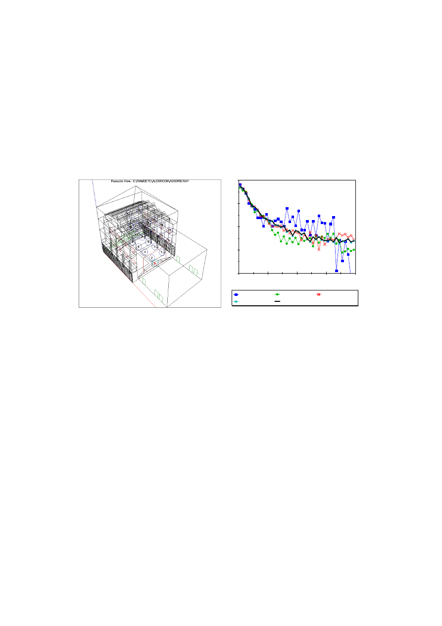
In figure 6 both the geometry and the results are reported for this case: it is the
Theatre Buero Vallejo recently built in Spain, at Alcorcon (near Madrid), with
architectural project of Isicio Ruiz. The simulation is representing the hall
completely furnished, while the stage is empty (and reverberating) at all.

The graph in fig. 6 shows the Impulse Response (not integrated) in the

octave band of 1 kHz obtained in receiver # 19 with the Ray Tracing program
and with Ramsete at various number of pyramids, the latter being corrected
with

α

=5.78 and

β

=0.0153. The double slope of the decay is quite evident.

40

50

60

70

80

Sound Pressure Level (dB)

0

0.5

1

1.5

2

Time (s)

64 Pyramids

256 Pyramids

1024 Pyramids

4096 pyramids

100000 Rays

Fig. 6 - Geometry (left) and Impulse Responses (right) of coupled volumes

In this case the results show very large discrepancies with 64 Pyramids,

and also with 256 pyramids the results are quite poor. Nevertheless, increasing
the number of pyramids to 1024 or more, the responses become practically
indistinguishable from the Ray Tracing results, while the computation times are
still reasonable (7min+43s for 1024 pyramids on a 486 DX-2 66 MHz) .

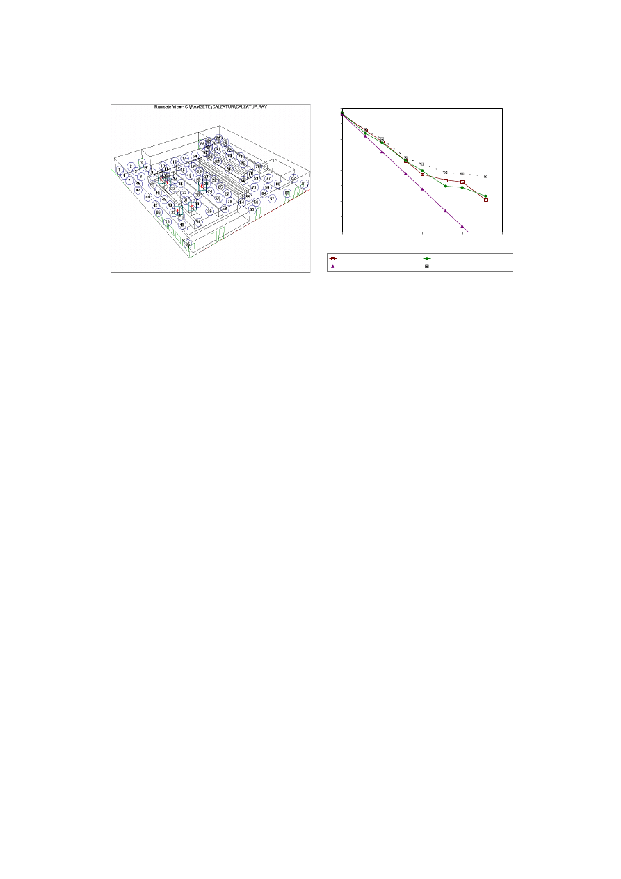
2.3 A very low room with non uniform absorption

Figure 7 show both the geometry and the results obtained: being the room

a typical industrial building, the most interesting acoustic property in this case
is the SPL decrement (in dBA) with the source-receiver distance.

The reference results (ray tracing, 160000 rays) are compared with a

single run of Ramsete (1024 pyramids), presented here with two different sets
of the post-processing coefficients

α

and

β

. The first set (Ramsete1,

α

=1.6,

β

=0.2) produces results very similar to the ray tracing.

80

85

90

95

100

Sound Pressure Level (dBA)

0

1

2

3

4

Number of distance doublings

Ray Tracing: 3.55 dB/doubling

Ramsete1: 3.65 dB/doubling

Free Field: 6.0 dB/doubling

Ramsete2: 2.91 dB/doubling

Figure 7 - A very low industrial building (with absorbing ceiling)

It must also be noted how adopting wrong values of

α

and

β

(Ramsete2)

causes large SPL differences only in points very far from the source: the dotted
line in fig. 7 is relative to the Sabinian values of

α

and

β

(2.0 and 0.3

respectively), and this overestimates the sound level of a maximum of 3.8 dB.

3. Conclusions

The pyramid tracing algorithm has the main advantage of being very fast, but
the tail correction required is quite delicate. As it was shown here, a proper
adjustment of the post-processing parameters

α

and

β

is required to obtain

results comparable with a “reference” (and very slow) Ray Tracing program.

The values of the parameters that produce good results can be obtained

with the simple rule used for the above cases:

α

and

β

were chosen as the

values that minimise the sum of squared differences between the results
obtained with two different pyramid generations (i.e. 256 and 4096 pyramids).

An automatic adjusting utility is actually being implemented to make this

“self-calibration” easy for everyone.

References

1. Farina, A. RAMSETE - a new Pyramid Tracer for medium and large scale

acoustic problems, Proc. of Euro-Noise 95, Lyon, France 21-23 march 1995.

2. Farina A., Cocchi A., Garai M., Semprini G., Old churches as concert halls: a

non-sabinian approach to optimum design of acoustic correction, F5-7, Proc. of
14

th

ICA, Beijing , China, 1992.

3. Farina, A. & Maffei, L. Sound Propagation Outdoor: Comparison between

Numerical Previsions and Experimental Results, in COMACO95, Proc. of Int.
Conf. on Comput. Acoustics and its Environmental Applications, Southampton,
England, 1995, Computational Mechanics Publications, Southampton 1995.

3.

Verbandt F.J.R., Jonckheere R.E., Bench-mark of acoustical ray-tracing

computer programs, Proc. of INTERNOISE 93, Leuven, Belgium, 1993.

4. Lewers T. A combined Beam Tracing and Radiant Exchange computer model of

Room Acoustics, Applied Acoustics, 1993,Vol. 38, no.s 2-4, pag. 161-176.