The Trillia Lectures on Mathematics
An Introduction to the Theory of Numbers
9 781931 705011

The Trillia Lectures on Mathematics
An Introduction to the
Theory of Numbers
Leo Moser
The Trillia Group
West Lafayette, IN

Terms and Conditions
You may download, print, transfer, or copy this work, either electronically
or mechanically, only under the following conditions.
If you are a student using this work for self-study, no payment is required.
If you are a teacher evaluating this work for use as a required or recommended
text in a course, no payment is required.
Payment is required for any and all other uses of this work. In particular,
but not exclusively, payment is required if
(1) you are a student and this is a required or recommended text for a course;
(2) you are a teacher and you are using this book as a reference, or as a
required or recommended text, for a course.
Payment is made through the website http://www.trillia.com. For each
individual using this book, payment of US$10 is required. A sitewide payment
of US$300 allows the use of this book in perpetuity by all teachers, students,
or employees of a single school or company at all sites that can be contained
in a circle centered at the location of payment with a radius of 25 miles (40
kilometers). You may post this work to your own website or other server (FTP,
etc.) only if a sitewide payment has been made and it is noted on your website
(or other server) precisely which people have the right to download this work
according to these terms and conditions.
Any copy you make of this work, by any means, in whole or in part, must
contain this page, verbatim and in its entirety.
An Introduction to the Theory of Numbers
c
1957 Leo Moser
ISBN 1-931705-01-1
Published by The Trillia Group, West Lafayette, Indiana, USA
First published: March 1, 2004. This version released: March 1, 2004.
The phrase “The Trillia Group” and The Trillia Group logo are trademarks of The Trillia
Group.
This book was prepared by William Moser from a manuscript by Leo Moser. We thank
Sinan Gunturk and Joseph Lipman for proofreading parts of the manuscript. We intend to
correct and update this work as needed. If you notice any mistakes in this work, please send
e-mail to lucier@math.purdue.edu and they will be corrected in a later version.

Contents
Preface
. . . . . . . . . . . . . . . . . . . . . . . . . . . . . . . . . . . . . . . . . . . . . . . . . . . . . . . . . . . . . . . . . . .
Chapter 1.
Compositions and Partitions
. . . . . . . . . . . . . . . . . . . . . . . . . . . . . .
Chapter 2.
Arithmetic Functions
. . . . . . . . . . . . . . . . . . . . . . . . . . . . . . . . . . . . . .
Chapter 3.
Distribution of Primes
. . . . . . . . . . . . . . . . . . . . . . . . . . . . . . . . . . .
Chapter 4.
Irrational Numbers
. . . . . . . . . . . . . . . . . . . . . . . . . . . . . . . . . . . . . . .
Chapter 5.
Congruences
. . . . . . . . . . . . . . . . . . . . . . . . . . . . . . . . . . . . . . . . . . . . . .
Chapter 6.
Diophantine Equations
. . . . . . . . . . . . . . . . . . . . . . . . . . . . . . . . . . .
Chapter 7.
Combinatorial Number Theory
. . . . . . . . . . . . . . . . . . . . . . . . . .
Chapter 8.
Geometry of Numbers
. . . . . . . . . . . . . . . . . . . . . . . . . . . . . . . . . . .
Classical Unsolved Problems
. . . . . . . . . . . . . . . . . . . . . . . . . . . . . . . . . . . . . . . . . . .
Miscellaneous Problems
. . . . . . . . . . . . . . . . . . . . . . . . . . . . . . . . . . . . . . . . . . . . . . . .
Unsolved Problems and Conjectures
. . . . . . . . . . . . . . . . . . . . . . . . . . . . . . . . . .


Preface
These lectures are intended as an introduction to the elementary theory of
numbers. I use the word “elementary” both in the technical sense—complex
variable theory is to be avoided—and in the usual sense—that of being easy to
understand, I hope.
I shall not concern myself with questions of foundations and shall presuppose
familiarity only with the most elementary concepts of arithmetic, i.e., elemen-
tary divisibility properties, g.c.d. (greatest common divisor), l.c.m. (least com-
mon multiple), essentially unique factorizaton into primes and the fundamental
theorem of arithmetic: if p
| ab then p | a or p | b.
I shall consider a number of rather distinct topics each of which could easily
be the subject of 15 lectures. Hence, I shall not be able to penetrate deeply
in any direction. On the other hand, it is well known that in number theory,
more than in any other branch of mathematics, it is easy to reach the frontiers
of knowledge. It is easy to propound problems in number theory that are
unsolved. I shall mention many of these problems; but the trouble with the
natural problems of number theory is that they are either too easy or much
too difficult. I shall therefore try to expose some problems that are of interest
and unsolved but for which there is at least a reasonable hope for a solution
by you or me.
The topics I hope to touch on are outlined in the Table of Contents, as are
some of the main reference books.
Most of the material I want to cover will consist of old theorems proved in
old ways, but I also hope to produce some old theorems proved in new ways
and some new theorems proved in old ways. Unfortunately I cannot produce
many new theorems proved in really new ways.

Chapter 1
Compositions and Partitions
We consider problems concerning the number of ways in which a number can
be written as a sum. If the order of the terms in the sum is taken into account
the sum is called a composition and the number of compositions of n is denoted
by c(n). If the order is not taken into account the sum is a partition and the
number of partitions of n is denoted by p(n). Thus, the compositions of 3 are
3 = 3, 3 = 1 + 2, 3 = 2 + 1, and 3 = 1 + 1 + 1,
so that c(3) = 4. The partitions of 3 are
3 = 3, 3 = 2 + 1, and 3 = 1 + 1 + 1,
so p(3) = 3.
There are essentially three methods of obtaining results on compositions
and partitions. First by purely combinatorial arguments, second by algebraic
arguments with generating series, and finally by analytic operations on the
generating series. We shall discuss only the first two of these methods.
We consider first compositions, these being easier to handle than partitions.
The function c(n) is easily determined as follows. Consider n written as a sum
of 1’s. We have n
− 1 spaces between them and in each of the spaces we can
insert a slash, yielding 2
n
−1
possibilities corresponding to the 2
n
−1
composition
of n. For example
3 = 1 1 1, 3 = 1/1 1, 3 = 1 1/1, 3 = 1/1/1.
Just to illustrate the algebraic method in this rather trivial case we consider
∞
X
n=1
c(n)x
n
.
It is easily verified that
∞
X
n=1
c(n)x
n
=
∞
X
m=1
(x + x
2
+ x
3
+
· · · )
m
=
∞
X
m=1
x
1
− x
m
=
x
1
− 2x
=
∞
X
n=1
2
n
−1
x
n
.
2
Chapter 1. Compositions and Partitions
Examples.
As an exercise I would suggest using both the combinatorial method and
the algebraic approach to prove the following results:
(1) The number of compositions of n into exactly m parts is
n
− 1
m
− 1
(Catalan);
(2) The number of compositions of n into even parts is 2
n
2
− 1
if n is
even and 0 if n is odd;
(3) The number of compositions of n into an even number of parts is
equal to the number of compositions of n into an odd number of
parts.
Somewhat more interesting is the determination of the number of composi-
tions c
∗
(n) of n into odd parts. Here the algebraic approach yields
X
n=1
c
∗
(n)x
n
=
∞
X
m=1
(x + x
3
+ x
5
+
· · · )
m
=
∞
X
m=1
x
1
− x
2
m
=
x
1
− x − x
2
=
X
F (n)x
n
.
By cross multiplying the last two expressions we see that
F
n+2
= F
n
+ F
n+1
, F
0
= 1, F
1
= 1.
Thus the F ’s are the so-called Fibonacci numbers
1, 1, 2, 3, 5, 8, 13, . . . .
The generating function yields two explicit expressions for these numbers.
First, by “partial fractioning”
x
1
−x−x
2
, expanding each term as a power se-
ries and comparing coefficients, we obtain
F
n
=
1
√
5
(
1 +
√
5
2
!
n
−
1
−
√
5
2
!
n
)
.
Another expression for F
n
is obtained by observing that
x
1
− x − x
2
= x(1 + (x + x
2
)
1
+ (x + x
2
)
2
+ (x + x
2
)
3
+
· · · ).
Comparing the coefficients here we obtain (Lucas)
F
n
=
n
− 1
0
+
n
− 2
1
+
n
− 3
2
+
· · · .
You might consider the problem of deducing this formula by combinatorial
arguments.
Chapter 1. Compositions and Partitions
3
Suppose we denote by a(n) the number of compositions of n with all sum-
mands at most 2, and by b(n) the number of compositions of n with all sum-
mands at least 2. An interesting result is that a(n) = b(n + 2). I shall prove
this result and suggest the problem of finding a reasonable generalization.
First note that a(n) = a(n
− 1) + a(n − 2). This follows from the fact that
every admissible composition ends in 1 or 2. By deleting this last summand,
we obtain an admissible composition of n
− 1 and n − 2 respectively. Since
a(1) = 1 and a(2) = 2, it follows that a(n) = F
n
. The function b(n) satisfies
the same recursion formula. In fact, if the last summand in an admissible
composition of n is 2, delete it to obtain an admissible composition of n
− 2;
if the last summand is greater than 2, reduce it by 1 to obtain an admissible
composition of n
− 1. Since b(2) = b(3) = 1, it follows that b(n) = F
n
−2
so
that a(n) = F
n
= b(n + 2).
An interesting idea for compositions is that of weight of a composition.
Suppose we associate with each composition a number called the weight, which
is the product of the summands. We shall determine the sum w(n) of the
weights of the compositions of n. The generating function of w(n) is
∞
X
n=1
w(n)x
n
=
∞
X
m=1
(x + 2x
2
+ 3x
3
+
· · · )
m
=
x
1
− 3x + x
2
.
From this we find that w(n) = 3w(n
− 1) − w(n − 2). I leave it as an exercise
to prove from this that w(n) = F
2n
−1
.
We now turn to partitions. There is no simple explicit formula for p(n). Our
main objective here will be to prove the recursion formula
p(n) = p(n
− 1) + p(n − 2) − p(n − 5) − p(n − 7) + p(n − 12) + p(n − 15) + · · ·
discovered by Euler. The algebraic approach to partition theory depends on
algebraic manipulations with the generating function
∞
X
n=1
p(n)x
n
=
1
(1
− x)(1 − x
2
)(1
− x
3
)
· · ·
and related functions for restricted partitions. The combinatorial approach
depends on the use of partition (Ferrer) diagrams. For example the Ferrer
diagram of the partition 7 = 4 + 2 + 1 is
• • • •
• •
•
Useful here is the notion of conjugate partition. This is obtained by reflecting
the diagram in a 45
◦
line going down from the top left corner. For example,
4
Chapter 1. Compositions and Partitions
the partitions
• • • •
• •
•
and
• • •
• •
•
•
are conjugate to each other. This correspondence yields almost immediately
the following theorems:
The number of partitions of n into m parts is equal to the number of parti-
tions on n into parts the largest of which is m;
The number of partitions of n into not more than m parts is equal to the
number of partitions of n into parts not exceeding m.
Of a somewhat different nature is the following: The number of partitions
of n into odd parts is equal to the number of partitions of n into distinct parts.
For this we give an algebraic proof. Using rather obvious generating functions
for the required partitions the result comes down to showing that
1
(1
− x)(1 − x
2
)(1
− x
3
) . . .
= 1 + x
1
+ x
2
+ x
3
+
· · · .
Cross multiplying makes the result intuitive.
We now proceed to a more important theorem due to Euler:
(1
− x)(1 − x
2
)(1
− x
3
)
· · · = 1 − x
1
− x
2
+ x
5
+ x
7
− x
12
− x
15
+
· · · ,
where the exponents are the numbers of the form
1
2
k(3k
± 1). We first note
that
(1
− x)(1 − x
2
)(1
− x
3
)
· · · =
X
((E(n)
− O(n))x
n
,
where E(n) is the number of partitions of n into an even number of distinct
parts and O(n) the number of partitions of n into an odd number of distinct
parts.
We try to establish a one-to-one correspondence between partitions of the
two sorts considered. Such a correspondence naturally cannot be exact, since
an exact correspondence would prove that E(n) = O(n).
We take a graph representing a partition of n into any number of unequal
parts. We call the lowest line AB the base of the graph. From C, the extreme
north-east node, we draw the longest south-westerly line possible in the graph;
this may contain only one node. This line CDE is called the wing of the graph
• • • • • •
• C
• • • • • • D
• • • • • E
• • •
• •
A
B
.

Chapter 1. Compositions and Partitions
5
Usually we may move the base into position of a new wing (parallel and to
the right of the “old” wing). Sometimes we may carry out the reverse operation
(moving the wing to be over the base, below the old base). When the operation
described or its converse is possible, it leads from a partition with into an odd
number of parts into an even number of parts or conversely. Thus, in general
E(n) = O(n). However two cases require special attention,. They are typified
by the diagrams
• • • • • • •
• • • • • •
• • • • •
• • • •
and
• • • • • • • •
• • • • • • •
• • • • • •
• • • • •
.
In these cases n has the form
k + (k + 1) +
· · · + (2k − 1) =
1
2
(3k
2
− k)
and
(k + 1) + (k + 2) +
· · · + (2k) =
1
2
(3k
2
+ k).
In both these cases there is an excess of one partition into an even number
of parts, or one into an odd number, according as k is even or odd. Hence
E(n)
−O(n) = 0, unless n =
1
2
(3k
±k), when E(n) −O(n) = (−1)
k
. This gives
Euler’s theorem.
Now, from
X
p(n)x
n
(1
− x − x
2
+ x
5
+ x
7
− x
12
− · · · ) = 1
we obtain a recurrence relation for p(n), namely
p(n) = p(n
− 1) + p(n − 2) − p(n − 5) − p(n − 7) + p(n − 12) + · · · .


Chapter 2
Arithmetic Functions
The next topic we shall consider is that of arithmetic functions. These form
the main objects of concern in number theory. We have already mentioned two
such functions of two variables, the g.c.d. and l.c.m. of m and n, denoted by
(m, n) and [m, n] respectively, as well as the functions c(n) and p(n). Of more
direct concern at this stage are the functions
π(n) =
X
p
≤n
1
the number of primes n not exceeding n;
ω(n) =
X
p
|n
1
the number of distinct primes factors of n;
Ω(n) =
X
p
i
|n
1
the number of prime power factors of n;
τ (n) =
X
d
|n
1
the number of divisors of n;
σ(n) =
X
d
|n
d
the sum of the divisors of n
ϕ(n) =
X
(a,n)=1
1
≤a≤n
1
the Euler totient function;
the Euler totient function counts the number of integers
≤ n and relatively
prime to n.
In this section we shall be particularly concerned with the functions τ (n),
σ(n), and ϕ(n). These have the important property that if
n = ab and (a, b) = 1
then
f (ab) = f (a)f (b).
Any function satisfying this condition is called weakly multiplicative, or simply
multiplicative.
8
Chapter 2. Arithmetic Functions
A generalization of τ (n) and σ(n) is afforded by
σ
k
(n) =
X
d
|n
d
k
the sum of the k
th
powers of the divisors of n,
since σ
0
(n) = τ (n) and σ
1
(n) = σ(n).
The ϕ function can also be generalized in many ways. We shall consider
later the generalization due to Jordan, ϕ
k
(n) = number of k-tuples
≤ n whose
g.c.d. is relatively prime to n. We shall derive some elementary properties of
these and closely related functions and state some special solved and unsolved
problems concerning them. We shall then discuss a theory which gives a unified
approach to these functions and reveals unexpected interconnections between
them. Later we shall discuss the magnitude of these functions. The func-
tions ω(n), Ω(n), and, particularly, π(n) are of a different nature and special
attention will be given to them.
Suppose in what follows that the prime power factorization of n is given by
n = p
α
1
1
p
α
2
2
. . . p
α
s
s
or briefly n =
Y
p
α
.
We note that 1 is not a prime and take for granted the provable result that,
apart from order, the factorization is unique.
In terms of this factorization the functions σ
k
(n) and ϕ(n) are easily deter-
mined. It is not difficult to see that the terms in the expansion of the product
Y
p
|n
(1 + p
k
+ p
2k
+
· · · + p
αk
)
are precisely the divisors of n raised to the k
th
power. Hence we have the
desired expansion for σ
k
(n). In particular
τ (n) = σ
0
(n) =
Y
(α + 1),
and
σ(n) = σ
1
(n) =
Y
p
|n
(1 + p + p
2
+
· · · + p
α
) =
Y
p
|n
p
α+1
− 1
p
− 1
,
e.g., 60 = 2
2
· 3
1
· 5
1
,
τ (60) = (2 + 1)(1 + 1)(1 + 1) = 3
· 2 · 2 = 12,
σ(60) = (1 + 2 + 2
2
)(1 + 3)(1 + 5) = 7
· 4 · 6 = 168.
These formulas reveal the multiplicative nature of σ
k
(n).
To obtain an explicit formula for ϕ(n) we make use of the following well-
known combinatorial principle.
Chapter 2. Arithmetic Functions
9
The Principle of Inclusion and Exclusion.
Given N objects each of which which may or may not possess any of the
characteristics
A
1
, A
2
, . . . .
Let N (A
i
, A
j
, . . . ) be the number of objects having the characteristics
A
i
, A
j
, . . . and possibly others. Then the number of objects which have
none of these properties is
N
−
X
N (A
i
) +
X
i<j
N (A
i
, A
j
)
−
X
i<j<k
N (A
i
, A
j
, A
k
) +
· · · ,
where the summation is extended over all combinations of the subscripts
1, 2, . . . , n in groups of one, two, three and so on, and the signs of the
terms alternate.
An integer will be relatively prime to n only if it is not divisible by any of
the prime factors of n. Let A
1
, A
2
, . . . , A
s
denote divisibility by p
1
, p
2
, . . . , p
s
respectively. Then, according to the combinatorial principle stated above
ϕ(n) = n
−
X
i
n
p
i
+
X
i<j
n
p
i
p
j
−
X
i<j<k
n
p
i
p
j
p
k
+
· · · .
This expression can be factored into the form
ϕ(n) = n
Y
p
|n
1
−
1
p
,
e.g.,
ϕ(60) = 60
1
−
1
2
1
−
1
3
1
−
1
5
= 60
·
1
2
·
2
3
·
4
5
= 16.
A similar argument shows that
ϕ
k
(n) = n
k
Y
p
|n
1
−
1
p
k
.
The formula for ϕ(n) can also be written in the form
ϕ(n) = n
X
d
|n
µ(d)
d
,
where µ(d) takes on the values 0, 1,
−1. Indeed µ(d) = 0 if d has a square factor,
µ(1) = 1, and µ(p
1
p
2
. . . p
s
) = (
−1)
s
. This gives some motivation for defining
a function µ(n) in this way. This function plays an unexpectedly important
role in number theory.
Our definition of µ(n) reveals its multiplicative nature, but it it still seems
rather artificial. It has however a number of very important properties which
10
Chapter 2. Arithmetic Functions
can be used as alternative definitions. We prove the most important of these,
namely
X
d
|n
µ(d) =
1
if n = 1,
0
if n
6= 1.
Since µ(d) = 0 if d contains a squared factor, it suffices to suppose that n has
no such factor, i.e., n = p
1
p
2
. . . p
s
. For such an n > 1
X
d
|n
µ(d) = 1
−
n
1
+
n
2
− · · · = (1 − 1)
n
= 0.
By definition µ(1) = 1 so the theorem is proved.
If we sum this result over n = 1, 2, . . . , x, we obtain
x
X
d=1
j
x
d
k
µ(d) = 1,
which is another defining relation.
Another very interesting defining property, the proof of which I shall leave
as an exercise, is that if
M (x) =
x
X
d=1
µ(d)
then
x
X
d=1
M
j
x
d
k
= 1.
This is perhaps the most elegant definition of µ. Still another very important
property is that
∞
X
n=1
1
n
s
!
∞
X
n=1
µ(n)
n
s
!
= 1.
We now turn our attention to Dirichlet multiplication and series.
Consider the set of arithmetic functions. These can be combined in various
ways to give new functions. For example, we could define f + g by
(f + g)(n) = f (n) + g(n)
and
(f
· g)(n) = f(n) · g(n).
A less obvious mode of combination is given by f
× g, defined by
(f
× g)(n) =
X
d
|n
f (d)g
n
d
=
X
dd
0
=n
f (d)g(d
0
).

Chapter 2. Arithmetic Functions
11
This may be called the divisor product or Dirichlet product.
The motivation for this definition is as follows. If
F (s) =
∞
X
n=1
f (n)n
−s
, G(s) =
∞
X
n=1
g(n)n
−s
, and F (s)
· G(s) =
∞
X
n=1
h(n)n
−s
,
then it is readily checked that h = f
×g. Thus Dirichlet multiplication of arith-
metic functions corresponds to the ordinary multiplication of the corresponding
Dirichlet series:
f
× g = g × f, (f × g) × h = f × (g × h),
i.e., our multiplication is commutative and associative. A purely arithmetic
proof of these results is easy to supply.
Let us now define the function
` = `(n) : 1, 0, 0, . . . .
It is easily seen that f
× ` = f. Thus the function ` is the unity of our
multiplication.
It can be proved without difficulty that if f (1)
6= 0, then f has an inverse
with respect to `. Such functions are called regular. Thus the regular functions
form a group with respect to the operation
×.
Another theorem, whose proof we shall omit, is that the Dirichlet product
of multiplicative functions is again multiplicative.
We now introduce the functions
I
k
: 1
k
, 2
k
, 3
k
, . . . .
It is interesting that, starting only with the functions ` and I
k
, we can build
up many of the arithmetic functions and their important properties.
To begin with we may define µ(n) by µ = I
−1
0
. This means, of course, that
µ
× I
0
= ` or
X
d
|n
µ(d) = `(n),
and we have already seen that this is a defining property of the µ function. We
can define σ
k
by
σ
k
= I
0
× I
k
.
This means that
σ
k
(n) =
X
d
|n
d
k
· `(n),
which corresponds to our earlier definition. Special cases are
τ = I
0
× I
0
= I
2
0
and
σ = I
1
× I
1
12
Chapter 2. Arithmetic Functions
Further, we can define
ϕ
k
= µ
× I
k
= I
−1
0
× I
k
.
This means that
ϕ
k
(n) =
X
d
|n
µ(d)
n
d
k
,
which again can be seen to correspond to our earlier definition.
The special case of interest here is
ϕ = ϕ
1
= µ
× I
1
.
Now, to obtain some important relations between our functions, we note the
so-called M¨
obius inversion formula. From our point of view this says that
g = f
× I
0
⇐⇒ f = µ × g.
This is, of course, quite transparent. Written out in full it states that
g(n) =
X
d
|n
f (d)
⇔ f(n) =
X
d
|n
µ(d)g
n
d
.
In this form it is considerably less obvious.
Consider now the following applications. First
σ
k
= I
0
× I
k
⇐⇒ I
k
= µ
× σ
k
.
This means that
X
d
|n
µ(d)σ
k
n
d
= n
k
.
Important special cases are
X
d
|n
µ(d)τ
n
d
= 1,
and
X
d
|n
µ(d)σ
n
d
= n.
Again
ϕ
k
= I
−1
0
× I
k
⇐⇒ I
k
= I
0
× ϕ
k
,
so that
X
d
|n
ϕ
k
(d) = n
k
,
Chapter 2. Arithmetic Functions
13
the special case of particular importance being
X
d
|n
ϕ(n) = n.
We can obtain identities of a somewhat different kind. Thus
σ
k
× ϕ
k
= I
0
× I
k
× I
−1
0
× I
k
= I
k
× I
k
,
and hence
X
d
|n
σ
k
(d)ϕ
k
n
d
=
X
d
|n
d
k
n
d
k
=
X
d
|n
n
k
= τ (n)n
k
.
A special case of interest here is
X
d
|n
σ(d)ϕ
n
d
= nτ (n).
In order to make our calculus applicable to problems concerning distribution
of primes, we introduce a unary operation on our functions, called differentia-
tion:
f
0
(n) =
−f(n) log n.
The motivation for this definition can be seen from
d
ds
X
f (n)
n
s
=
−
X log nf(n)
n
s
.
Now let us define
Λ(n) =
log p
if n = p
α
,
0
if n
6= p
α
.
It is easily seen that
X
d
|n
Λ(n) = log n.
In our Dirichlet multiplication notation we have
Λ
× I
0
=
−I
0
0
,
so that
Λ = I
−1
0
× (−I
0
0
) = µ
× (−I
0
0
)
or
Λ(d) =
−
X
d
|n
µ(d) log
n
d
=
X
d
|n
µ(d) log d.
14
Chapter 2. Arithmetic Functions
Let us now interpret some of our results in terms of Dirichlet series. We
have the correspondence
F (s)
←→ f(n) if F (s) =
X f(n)
n
s
,
and we know that Dirichlet multiplication of arithmetic functions corresponds
to ordinary multiplication for Dirichlet series. We start with
f
←→ F, 1 ←→ 1, and I
0
←→ ζ(s).
Furthermore
I
k
←→
∞
X
n=1
n
k
n
s
= ζ(s
− k).
Also
µ
←→
1
ζ(s)
and
I
0
0
←→
X − log n
n
s
= ζ
0
(s).
This yields
X σ
k
(n)
n
s
= ζ(s)ζ(s
− k).
Special cases are
X τ(n)
n
s
= ζ
2
(s)
and
X σ(n)
n
s
= ζ(s)ζ(s
− 1).
Again
X ϕ(n)
n
s
=
1
ζ(s)
and
X ϕ
k
(n)
n
s
=
ζ(s
− k)
ζ(s)
,
with the special case
X ϕ(n)
n
s
=
ζ(s
− 1)
ζ(s)
.
To bring a few of these down to quite numerical results we have
X τ(n)
n
2
= ζ
2
(2) =
π
4
36
,
X σ
4
(n)
n
2
= ζ(2)
· ζ(4) =
π
2
6
·
π
4
90
=
π
6
540
,
X µ(n)
n
2
=
6
π
2
.
Chapter 2. Arithmetic Functions
15
As for our Λ function, we had
Λ = I
−1
0
× I
0
0
;
this means that
∞
X
n
−=1
Λ(n)
n
s
=
−ζ
0
(s)
ζ(s)
.
(
∗)
The prime number theorem depends on going from this to a reasonable estimate
for
Ψ(x) =
x
X
n=1
Λ(n).
Indeed we wish to show that Ψ(x)
∼ x.
Any contour integration with the right side of (
∗) involves of course the need
for knowing where ζ(s) vanishes. This is one of the central problems of number
theory.
Let us briefly discuss some other Dirichlet series.
If n = p
α
1
1
p
α
2
2
. . . p
α
s
s
define
λ(n) = (
−1)
α
1
+α
2
+
···+α
s
.
The λ function has properties similar to those of the µ function. We leave
as an exercise to show that
X
d
|n
λ(d) =
1
if n = r
2
,
0
if n
6= r
2
.
Now
ζ(2s) =
X s(n)
n
s
where s(n) =
1
if n = r
2
,
0
if n
6= r
2
.
Hence λ
× I
0
= s, i.e.,
X λ(n)
n
s
· ζ(s) = ζ(2s)
or
X λ(n)
n
s
=
ζ(2s)
ζ(s)
.
For example
X λ(n)
n
2
=
π
4
90
π
2
6
=
π
2
15
.
We shall conclude with a brief look at another type of generating series,
namely Lambert series. These are series of the type
X f(n)x
n
1
− x
n
.
16
Chapter 2. Arithmetic Functions
It is easily shown that if F = f
× I
0
then
X f(n)x
n
1
− x
n
=
X
F (n)x
n
.
Interesting special cases are
f = I
0
,
X x
n
1
− x
n
=
X
τ (n)x
n
;
f = µ,
X
µ(n)
x
n
1
− x
n
= x;
f = ϕ,
X
ϕ(n)
x
n
1
− x
n
=
X
nx
n
=
x
(1
− x)
2
.
For example, taking x =
1
10
in the last equality, we obtain
ϕ(1)
9
+
ϕ(2)
99
+
ϕ(3)
999
+
· · · =
10
81
.
Exercises.
Prove that
∞
X
n=1
µ(n)x
n
1 + x
n
= x
− 2x
2
.
Prove that
∞
X
n=1
λ(n)x
n
1
− x
n
=
∞
X
n=1
x
n
2
.
Chapter 3
Distribution of Primes
Perhaps the best known proof in all of “real” mathematics is Euclid’s proof of
the existence of infinitely many primes.
If p were the largest prime then (2
· 3 · 5 · · · p) + 1 would not be divisible by
any of the primes up to p and hence would be the product of primes exceeding
p.
In spite of its extreme simplicity this proof already raises many exceedingly
difficult questions, e.g., are the numbers (2
· 3 · . . . · p) + 1 usually prime or
composite? No general results are known. In fact, we do not know whether an
infinity of these numbers are prime, or whether an infinity are composite.
The proof can be varied in many ways. Thus, we might consider (2
· 3 ·
5
· · · p) − 1 or p! + 1 or p! − 1. Again almost nothing is known about how
such numbers factor. The last two sets of numbers bring to mind a problem
that reveals how, in number theory, the trivial may be very close to the most
abstruse. It is rather trivial that for n > 2, n!
−1 is not a perfect square. What
can be said about n! + 1? Well, 4! + 1 = 5
2
, 5! + 1 = 11
2
and 7! + 1 = 71
2
.
However, no other cases are known; nor is it known whether any other numbers
n! + 1 are perfect squares. We will return to this problem in the lectures on
diophantine equations.
After Euclid, the next substantial progress in the theory of distribution of
primes was made by Euler. He proved that
P
1
p
diverges, and described this
result by saying that the primes are more numerous than the squares. I would
like to present now a new proof of this fact—a proof that is somewhat related
to Euclid’s proof of the existence of infinitely many primes.
We need first a (well known) lemma concerning subseries of the harmonic
series. Let p
1
< p
2
< . . . be a sequence of positive integers and let its counting
function be
π(x) =
X
p
≤x
1.
Let
R(x) =
X
p
≤x
1
p
.
18
Chapter 3. Distribution of Primes
Lemma. If R(
∞) exists then
lim
x
→∞
π(x)
x
= 0.
Proof.
π(x) = 1(R(1)
− R(0)) + 2((R(2) − R(1)) + · · · + x(R(x) − R(x − 1)),
or
π(x)
x
= R(x)
−
R(0) + R(1) +
· · · + R(x − 1)
x
.
Since R(x) approaches a limit, the expression within the square brackets ap-
proaches this limit and the lemma is proved.
In what follows we assume that the p’s are the primes.
To prove that
P
1
p
diverges we will assume the opposite, i.e.,
P
1
p
converges
(and hence also that
π(x)
x
→ 0) and derive a contradiction.
By our assumption there exists an n such that
X
p>n
1
p
<
1
2
.
(1)
But now this n is fixed so there will also be an n such that
π(n! m)
n! m
<
1
2n!
.
(2)
With such an n and m we form the m numbers
T
1
= n!
− 1, T
2
= 2n!
− 1, . . . , T
m
= mn!
− 1.
Note that none of the T ’s have prime factors
≤ n or ≥ mn!. Furthermore if
p
| T
i
and p
| T
j
then p
| (T
i
− T
j
) so that p
| (i − j). In other words, the
multiples of p are p apart in our set of numbers. Hence not more than
m
p
+ 1
of the numbers are divisible by p. Since every number has at least one prime
factor we have
X
n<p<n! m
m
p
+ 1
≥ m
or
X
n<p
1
p
+
π(n! m)
m
≥ 1.
But now by (1) and (2) the right hand side should be < 1 and we have a
contradiction, which proves our theorem.
Chapter 3. Distribution of Primes
19
Euler’s proof, which is more significant, depends on his very important iden-
tity
ζ(s) =
∞
X
n=1
1
n
s
=
Y
p
1
1
−
1
p
s
.
This identity is essentially an analytic statement of the unique factorization
theorem. Formally, its validity can easily be seen. We have
Y
p
1
1
−
1
p
s
=
Y
p
1 +
1
p
s
+
1
p
2s
+
· · ·
=
1 +
1
2
s
+
· · ·
1 +
1
3
s
+
· · ·
1 +
1
5
s
+
· · ·
=
1
1
s
+
1
2
s
+
1
3
s
+
· · · .
Euler now argued that for s = 1,
∞
X
n=1
1
n
s
=
∞
so that
Y
p
1
1
−
1
p
must be infinite, which in turn implies that
P
1
p
must be infinite.
This argument, although not quite valid, can certainly be made valid. In
fact, it can be shown without much difficulty that
X
n
≤x
1
n
−
Y
p
≤x
1
−
1
p
−1
is bounded. Since
X
n
≤x
1
n
− log x is bounded, we can, on taking logs, obtain
log log x =
X
p
≤x
− log
1
−
1
p
+ O(1)
so that
X
p
≤x
1
p
= log log x + O(1).
We shall use this result later.
20
Chapter 3. Distribution of Primes
Gauss and Legendre were the first to make reasonable estimates for π(x).
Essentially, they conjectured that
π(x)
∼
x
log x
,
the famous Prime Number Theorem. Although this was proved in 1896 by J.
Hadamard and de la Vallee Poussin, the first substantial progress towards this
result is due to Chebycheff. He obtained the following three main results:
(1) There is a prime between n and 2n (n > 1);
(2) There exist positive constants c
1
and c
2
such that
c
2
x
log x
< π(x) <
c
1
x
log x
;
(3) If
π(x)
log x
approaches a limit, then that limit is 1.
We shall prove the three main results of Chebycheff using his methods as mod-
ified by Landau, Erd˝
os and, to a minor extent, L. Moser.
We require a number of lemmas. The first of these relate to the magnitude
of
n! and
2n
n
.
As far as n! is concerned, we might use Stirling’s approximation
n!
∼ n
n
e
−n
√
2πn.
However, for our purposes a simpler estimate will suffice. Since
n
n
n!
is only one term in the expansion of e
n
,
e
n
>
n
n
n!
and we have the following lemma.
Lemma 1. n
n
e
−n
< n! < n
n
.
Since
(1 + 1)
2n
= 1 +
2n
1
+
· · · +
2n
n
+
· · · + 1,
it follows that
2n
n
< 2
2n
= 4
n
.
Chapter 3. Distribution of Primes
21
This estimate for
2n
n
is not as crude as it looks, for it can be easily seen from
Stirling’s formula that
2n
n
∼
4
n
√
πn
.
Using induction we can show that
2n
n
>
4
n
2n
,
and thus we have
Lemma 2.
4
n
2n
<
2n
n
< 4
n
.
Note that
2n+1
n
is one of two equal terms in the expansion of (1 + 1)
2n+1
.
Hence we also have
Lemma 3.
2n + 1
n
< 4
n
.
As an exercise you might use these to prove that if
n = a + b + c +
· · ·
then
n!
a! b! c!
· · ·
<
n
n
a
a
b
b
c
c
· · ·
.
Now we deduce information on how n! and
2n
n
factor as the product of
primes. Suppose e
p
(n) is the exponent of the prime p in the prime power
factorization of n!, i.e.,
n! =
Y
p
e
p
(n)
.
We easily prove
Lemma 4 (Legendre). e
p
(n) =
n
p
+
n
p
2
+
n
p
3
+
· · · .
In fact
j
n
p
k
is the number of multiples of p in n!, the term
j
n
p
2
k
adds the
additional contribution of the multiples of p
2
, and so on, e.g.,
e
3
(30) =
30
3
+
30
9
+
30
27
+
· · · = 10 + 3 + 1 = 14.
An interesting and sometimes useful alternative expression for e
p
(n) is given
by
e
p
(n) =
n
− s
p
(n)
p
− 1
,
22
Chapter 3. Distribution of Primes
where s
p
(n) represents the sum of the digits of n when n is expressed in base p.
Thus in base 3, 30 can be written 1010 so that e
3
(30) =
30
−2
2
= 14 as before.
We leave the proof of the general case as an exercise.
We next consider the composition of
2n
n
as a product of primes. Let E
p
(n)
denote the exponent of p in
2n
n
, i.e.,
2n
n
=
Y
p
p
E
p
(n)
.
Clearly
E
p
(n) = e
p
(2n)
− 2e
p
(n) =
X
i
2n
p
i
− 2
n
p
i
.
Our alternative expression for e
p
(n) yields
E
p
(n) =
2s
p
(n)
− s
p
(2n)
p
− 1
.
In the first expression each term in the sum can easily be seen to be 0 or 1 and
the number of terms does not exceed the exponent of the highest power of p
that does not exceed 2n. Hence
Lemma 5. E
p
(n)
≤ log
p
(2n).
Lemma 6. The contribution of p to
2n
n
does not exceed 2n.
The following three lemmas are immediate.
Lemma 7. Every prime in the range n < p < 2n appears exactly once in
2n
n
.
Lemma 8. No prime in the range
2n
3
< p < n is a divisor of
2n
n
.
Lemma 9. No prime in the range p >
√
2n appears more than once in
2n
n
.
Although it is not needed in what follows, it is amusing to note that since
E
2
(n) = 2s
2
(n)
− s
2
(2n) and s
2
(n) = s
2
(2n), we have E
2
(n) = s
2
(n).
As a first application of the lemmas we prove the elegant result
Theorem 1.
Y
p
≤n
p < 4
n
.
The proof is by induction on n. We assume the theorem true for integers
< n and consider the cases n = 2m and n = 2m + 1. If n = 2m then
Y
p
≤2m
p =
Y
p
≤2m−1
p < 4
2m
−1
Chapter 3. Distribution of Primes
23
by the induction hypothesis. If n = 2m + 1 then
Y
p
≤2m+1
p =
Y
p
≤m+1
p
Y
m+1<p<2m+1
p
!
< 4
m+1
2m + 1
m
≤ 4
m+1
4
m
= 4
2m+1
and the induction is complete.
It can be shown by much deeper methods (Rosser) that
Y
p
≤n
p < (2.83)
n
.
Actually the prime number theorem is equivalent to
X
p
≤n
log p
∼ n.
From Theorem 1 we can deduce
Theorem 2. π(n) <
cn
log n
.
Clearly
4
n
>
Y
p
≤n
p >
Y
√
n
≤p≤n
p >
√
n
π(n)
−π(
√
n)
Taking logarithms we obtain
n log 4 > (π(n)
− π(
√
n))
1
2
log n
or
π(n)
− π(
√
n) <
n
· 4 log 2
log n
or
π(n) < (4 log 2)
n
log n
+
√
n <
cn
log n
.
Next we prove
Theorem 3. π(n) >
cn
log n
.
For this we use Lemmas 6 and 2. From these we obtain
(2n)
π(2n)
>
2n
n
>
4
n
2n
.
Taking logarithms, we find that
(π(n) + 1) log 2n > log(2
2n
) = 2n log 2.
24
Chapter 3. Distribution of Primes
Thus, for even m
π(m) + 1 >
m
log m
log 2
and the result follows.
We next obtain an estimate for S(x) =
X
p
≤x
log p
p
. Taking the logarithm of
n! =
Q
p
p
e
p
we find that
n log n > log n! =
X
e
p
(n) log p > n(log n
− 1).
The reader may justify that the error introduced in replacing e
p
(n) by
n
p
(of
course e
p
(n) =
P j
n
p
i
k
) is small enough that
X
p
≤n
n
p
log p = n log n + O(n)
or
X
p
≤n
log p
p
= log n + O(1).
We can now prove
Theorem 4. R(x) =
X
p
≤x
1
p
= log log x + O(1).
In fact
R(x) =
x
X
n=2
S(n)
− S(n − 1)
log n
=
x
X
n=2
S(n)
1
log n
−
1
log(n + 1)
+ O(1)
=
x
X
n=2
(log n + O(1))
log(1 +
1
n
)
(log n) log(n + 1)
+ O(1)
=
x
X
n=2
1
n log n
+ O(1)
= log log x + O(1),
as desired.
We now outline the proof of Chebycheff’s
Theorem 5. If π(x)
∼
cx
log x
, then c = 1.
Chapter 3. Distribution of Primes
25
Since
R(x) =
x
X
n=1
π(n)
− π(n − 1)
n
=
x
X
n=1
π(n)
n
2
+ O(1),
π(n)
∼
cx
log x
would imply
x
X
n=1
π(n)
n
2
∼ c log log x.
But we already know that π(x)
∼ log log x so it follows that c = 1.
We next give a proof of Bertrand’s Postulate developed about ten years ago
(L. Moser). To make the proof go more smoothly we only prove the somewhat
weaker
Theorem 6. For every integer r there exists a prime p with
3
· 2
2r
−1
< p < 3
· 2
2r
.
We restate several of our lemmas in the form in which they will be used.
(1) If n < p < 2n then p occurs exactly once in
2n
n
.
(2) If 2
· 2
2r
−1
< p < 3
· 2
2r
−1
then p does not occur in
3
· 2
2r
3
· 2
2r
−1
.
(3) If p > 2
r+1
then p occurs at most once in
3
· 2
n
3
· 2
n
−1
.
(4) No prime occurs more than 2r + 1 times in
3
· 2
r
3
· 2
2r
−1
.
We now compare
3
· 2
2r
3
· 2
2r
−1
and
2
2r
2
2r
−1
2
2r
−1
2
2r
−2
. . .
2
1
2
r+1
2
r
2
r
2
r
−1
· · · · ·
2
1
2r
.
Assume that there is no prime in the range 3
· 2
2r
−1
< p < 3
· 2
2r
. Then, by
our lemmas, we find that every prime that occurs in the first expression also
occurs in the second with at least as high a multiplicity; that is, the second
expression in not smaller than the first. On the other hand, observing that for
r
≥ 6
3
· 2
2r
> (2
2r
+ 2
2r
−1
+
· · · + 2) + 2r(2
r+1
+ 2
r
+
· · · + 2),
26
Chapter 3. Distribution of Primes
and interpreting
2n
n
as the number of ways of choosing n objects from 2n,
we conclude that the second expression is indeed smaller than the first. This
contradiction proves the theorem when r > 6. The primes 7, 29, 97, 389, and
1543 show that the theorem is also true for r
≤ 6.
The proof of Bertrand’s Postulate by this method is left as an exercise.
Bertrand’s Postulate may be used to prove the following results.
(1)
1
2
+
1
3
+
· · · +
1
n
is never an integer.
(2) Every integer > 7 can be written as the sum of distinct primes.
(3) Every prime p
n
can be expressed in the form
p
n
=
±2 ± 3 ± 5 ± · · · ± p
n
−1
with an error of at most 1 (Scherk).
(4) The equation π(n) = ϕ(n) has exactly 8 solutions.
About 1949 a sensation was created by the discovery by Erd˝
os and Selberg
of an elementary proof of the Prime Number Theorem. The main new result
was the following estimate, proved in an elementary manner:
X
p
≤x
log
2
p +
X
pq
≤x
log p log q = 2x log x + O(x).
Although Selberg’s inequality is still far from the Prime Number Theorem,
the latter can be deduced from it in various ways without recourse to any
further number theoretical results. Several proofs of this lemma have been
given, perhaps the simplest being due to Tatuzawa and Iseki. Selberg’s original
proof depends on consideration of the functions
λ
n
= λ
n,x
=
X
d
|n
µ(d) log
2
x
d
and
T (x) =
x
X
n=1
λ
n
x
n
.
Some five years ago J. Lambek and L. Moser showed that one could prove
Selberg’s lemma in a completely elementary way, i.e., using properties of inte-
gers only. One of the main tools for doing this is the following rational analogue
of the logarithm function. Let
h(n) = 1 +
1
2
+
1
3
+
· · · +
1
n
and
`
k
(n) = h(kn)
− h(k).
We prove in an quite elementary way that
|`
k
(ab)
− `
k
(a)
− `
k
(b)
| <
1
k
.
Chapter 3. Distribution of Primes
27
The results we have established are useful in the investigation of the magni-
tude of the arithmetic functions σ
k
(n), ϕ
k
(n) and ω
k
(n). Since these depend
not only on the magnitude of n but also strongly on the arithmetic structure
of n we cannot expect to approximate them by the elementary functions of
analysis. Nevertheless we shall will see that “on the average” these functions
have a rather simple behavior.
If f and g are functions for which
f (1) + f (2) +
· · · + f(n) ∼ g(1) + g(2) + · · · + g(n)
we say that f and g have the same average order. We will see, for example,
that the average order of τ (n) is log n, that of σ(n) is
π
2
6
n and that of ϕ(n) is
6
π
2
n.
Let us consider first a purely heuristic argument for obtaining the average
value of σ
k
(n). The probability that r
| n is
1
r
and if r
| n then
n
r
contributes
n
r
k
to σ
k
(n). Thus the expected value of σ
k
(n) is
1
1
n
1
k
+
1
2
n
2
k
+
· · · +
1
n
n
n
k
= n
k
1
1
k+1
+
1
2
k+1
+
· · · +
1
n
k+1
For k = 0 this will be about n log n. For n
≥ 1 it will be about n
k
ζ(k + 1),
e.g., for n = 1 it will be about nζ(2) = n
π
2
6
.
Before proceeding to the proof and refinement of some of these results we
consider some applications of the inversion of order of summation in certain
double sums.
Let f be an arithmetic function and associate with it the function
F (n) =
X
d
|n
f (d)
and g = f
× I, i.e.,
g(n) =
X
d
|n
f (d).
We will obtain two expressions for
F(x) =
x
X
n=1
g(n).
28
Chapter 3. Distribution of Primes
F(x) is the sum
f (1)
+
f (1)
+
f (2)
+
f (1)
+
f (3)
+
f (1)
+
f (2)
+
f (4)
+
f (1)
f (5)
+
f (1)
+
f (2)
+
f (3)
Adding along vertical lines we have
x
X
d=1
j
x
d
k
f (d);
if we add along the lines indicated we obtain
x
X
n=1
F
j
x
n
k
.
Thus
x
X
n=1
X
d
|n
f (d) =
x
X
d=1
j
x
d
k
f (d) =
x
X
n=1
F
j
x
n
k
.
The special case f = µ yields
1 =
x
X
d=1
µ(d)
j
x
d
k
=
x
X
n=1
M
j
x
n
k
,
which we previously considered.
From
x
X
d=1
µ(d)
j
x
d
k
= 1,
we have, on removing brackets, allowing for error, and dividing by x,
x
X
d=1
µ(d)
d
< 1.
Actually, it is known that
∞
X
d=1
µ(d)
d
= 0,
but a proof of this is as deep as that of the prime number theorem.
Next we consider the case f = 1. Here we obtain
x
X
n=1
τ (n) =
x
X
n=1
j
x
n
k
= x log x + O(x).
Chapter 3. Distribution of Primes
29
In the case f = I
k
we find that
x
X
n=1
σ
k
(n) =
x
X
d=1
d
k
j
x
d
k
=
x
X
n=1
1
k
+ 2
k
+
· · · +
j
x
n
k
k
.
In the case f = ϕ, recalling that
X
d
|n
ϕ(d) = n, we obtain
x(x + 1)
2
=
x
X
n=1
X
d
|n
ϕ(d) =
x
X
d=1
j
x
d
k
ϕ(d) =
x
X
n=1
Φ
x
n
,
where Φ(n) =
n
X
d=1
ϕ(d). From this we easily obtain
x
X
d=1
ϕ(d)
d
≥
x + 1
2
,
which reveals that, on the average, ϕ(d) >
d
2
.
One can also use a similar inversion of order of summation to obtain the
following important second M¨
obius inversion formula:
Theorem.
If G(x) =
x
X
n=1
F
j
x
n
k
then F (x) =
x
X
n=1
µ(n)G
j
x
n
k
.
Proof.
x
X
n=1
µ(n)G
j
x
n
k
=
x
X
n=1
µ(n)
bx/nc
X
n=1
F
j
x
mn
k
=
x
X
k=1
F
j
x
n
k
x
X
n
|k
µ(n) = F (x).
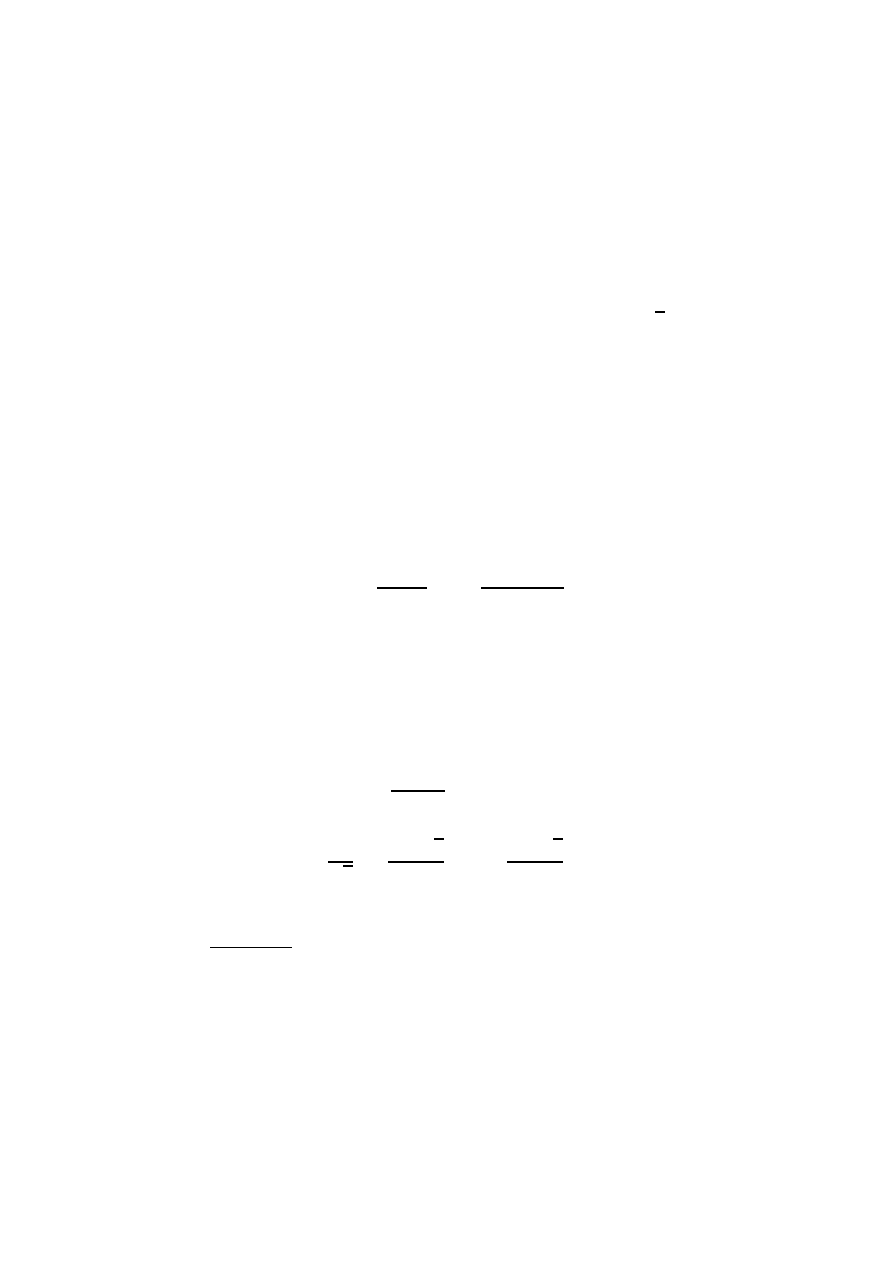
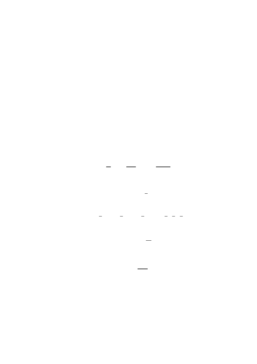
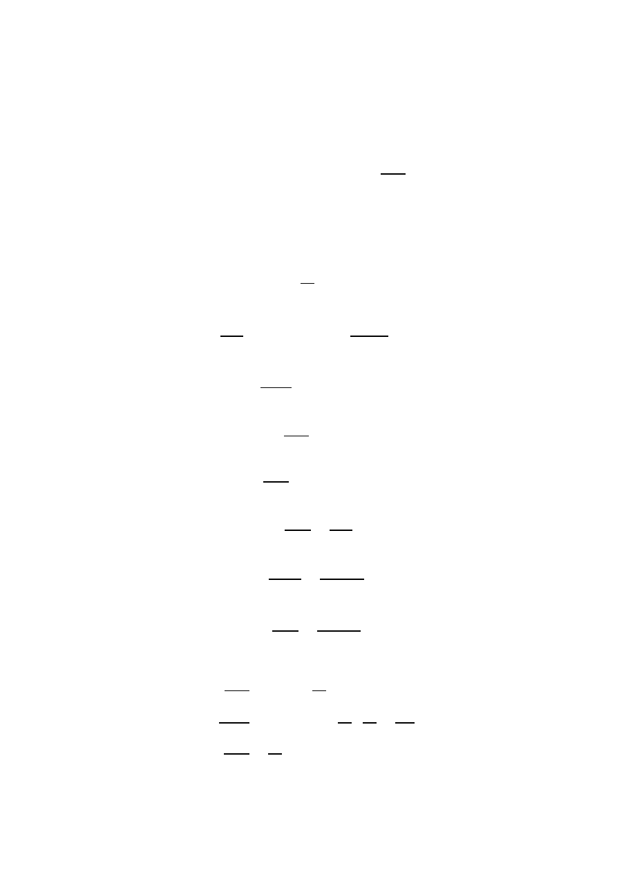
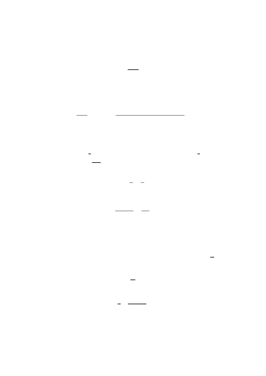
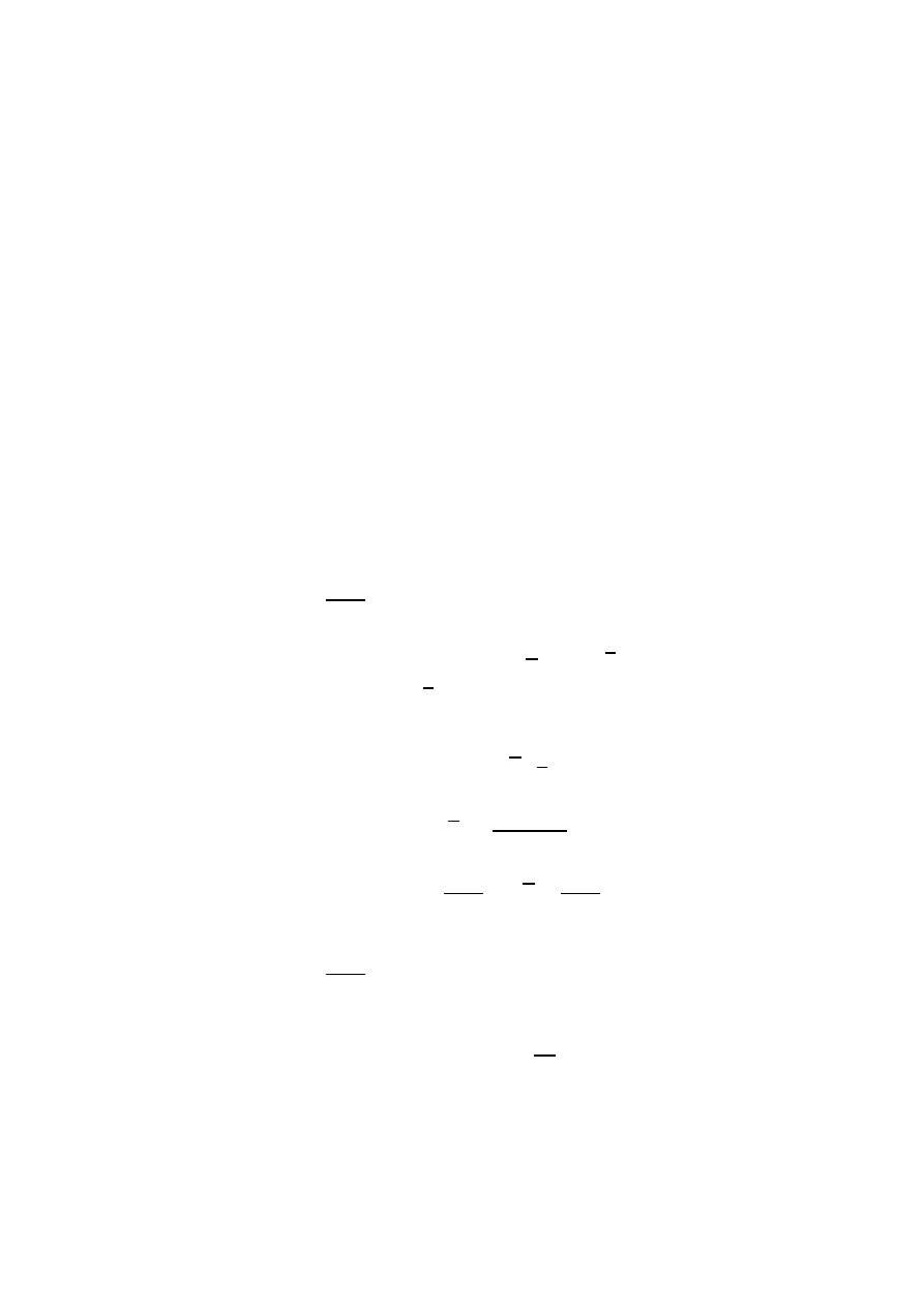
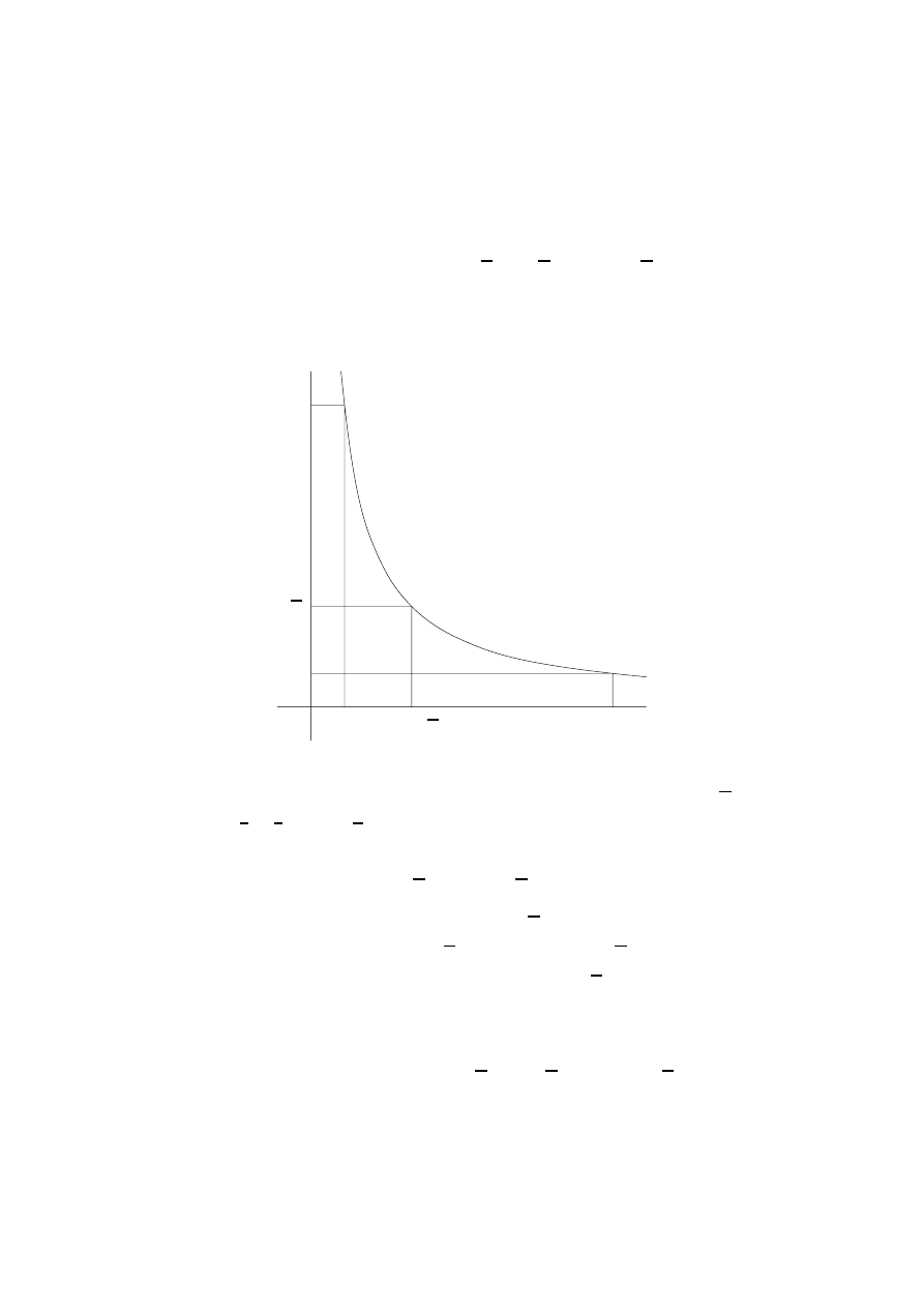
Consider again our estimate
τ (1) + τ (2) +
· · · + τ(n) = n log n + O(n).
It is useful to obtain a geometric insight into this result. Clearly τ (r) is the
number of lattice points on the hyperbola xy = r, x > 0, y > 0. Also, every
lattice point (x, y), x > 0, y > 0, xy
≤ n, lies on some hyperbola xy = r, r ≤ n.
Hence
n
X
r=1
τ (r)
30
Chapter 3. Distribution of Primes
is the number of lattice points in the region xy
≤ n, x > 0, y > 0. If we sum
along vertical lines x = 1, 2, . . . , n we obtain again
τ (1) + τ (2) +
· · · + τ(n) =
j
n
1
k
+
j
n
2
k
+
· · · +
j
n
n
k
.
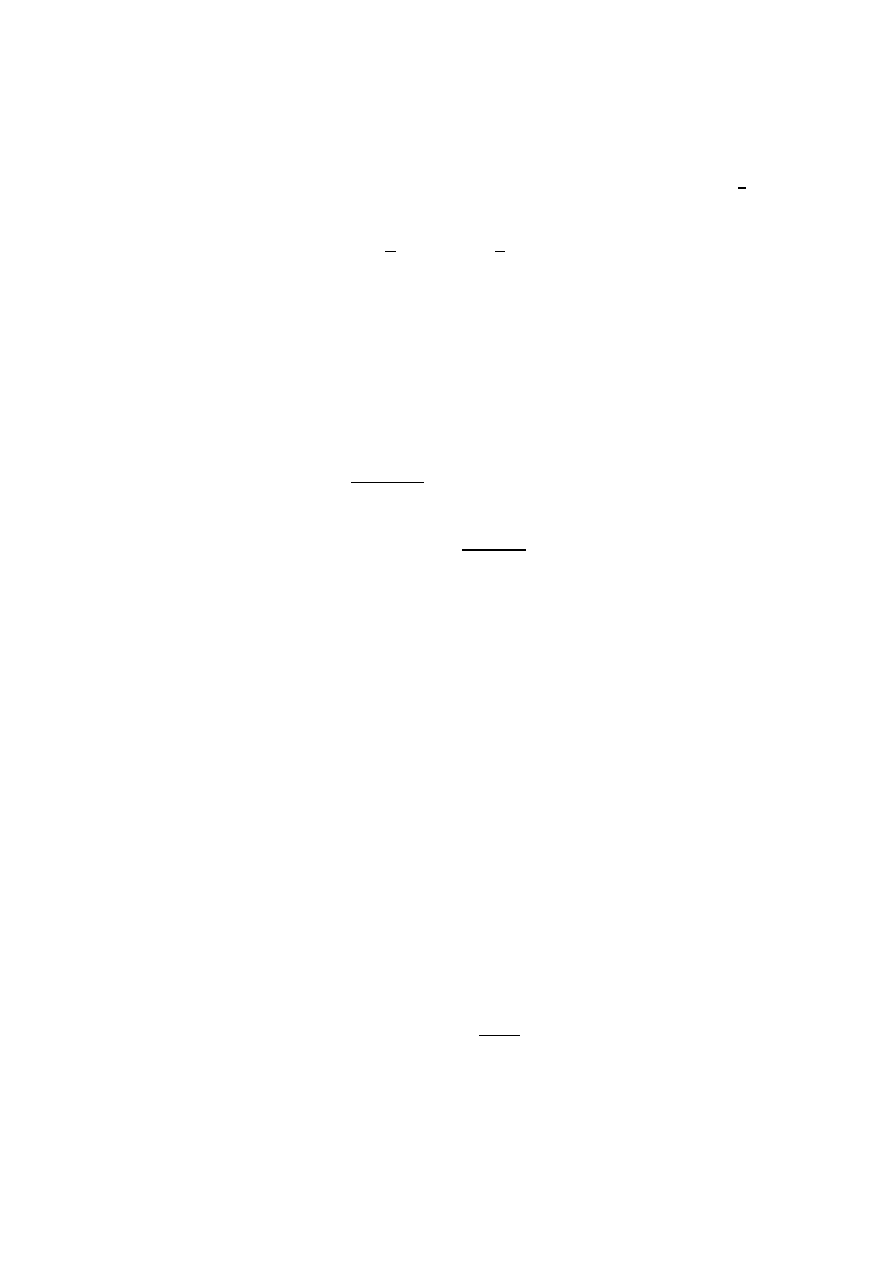
In this approach, the symmetry of xy = n about x = y suggests how to
improve this estimate and obtain a smaller error term.
x = 1
x =
√
n
y = 1
y =
√
n
xy = n
Figure 1
Using the symmetry of the above figure, we have, with u =
b
√
n
c and
h(n) = 1 +
1
2
+
1
3
+
· · · +
1
n
,
n
X
r=1
τ (r) = 2
j
n
1
k
+
· · · +
j
n
u
k
− u
2
= 2nh(u)
− n + O(
√
n)
= 2n log
√
u + (2γ
− 1)n + O(
√
n)
= n log n + (2γ
− 1)n + O(
√
n).
Proceeding now to
P
σ(r) we have
σ(1) + σ(2) +
· · · + σ(n) = 1
j
n
1
k
+ 2
j
n
2
k
+
· · · + n
j
n
n
k
.
In order to obtain an estimate of
x
X
n=1
σ(n) set k = 1 in the identity (obtained
Chapter 3. Distribution of Primes
31
earlier)
σ
k
(1) + σ
k
(2) +
· · · + σ
k
(x) =
x
X
n=1
1
k
+ 2
k
+
· · · +
j
x
n
k
k
.
We have immediately
σ(1) + σ(2) +
· · · + σ(x) =
1
2
x
X
n=1
j
x
n
k j
x
n
+ 1
k
=
1
2
∞
X
n=1
x
2
n
2
+ O(x log x) =
x
2
ζ(2)
2
+ O(x log x)
=
π
2
x
2
12
+ O(x log x).
To obtain similar estimates for ϕ(n) we note that ϕ(r) is the number of
lattice points that lie on the line segment x = r, 0 < y < r, and can be seen from
the origin. (A point (x, y) can be seen if (x, y) = 1.) Thus ϕ(1)+ϕ(2)+
· · ·+ϕ(n)
is the number of visible lattice points in the region with n > x > y > 0.
Let us consider a much more general problem, namely to estimate the num-
ber of visible lattice points in a large class of regions.
Heuristically we may argue as follows. A point (x, y) is invisible by virtue
of the prime p if p
| x and p | y. The probability that this occurs is
1
p
2
. Hence
the probability that the point is invisible is
Y
p
1
−
1
p
2
=
Y
p
1 +
1
p
2
+
1
p
4
+
· · ·
−1
=
1
ζ(2)
=
6
π
2
.
Thus the number of visible lattice point should be
6
π
2
times the area of the
region. In particular the average order of ϕ(n) should be about
6
π
2
n.
We now outline a proof of the fact that in certain large regions the fraction
of visible lattice points contained in the region is approximately
6
π
2
.
Le R be a region in the plane having finite Jordan measure and finite perime-
ter. Let tR denote the region obtained by magnifying R radially by t. Let
M (tR) be the area of tR, L(tR) the number of lattice points in tR, and V (tR)
the number of visible lattice points in tR.
It is intuitively clear that
L(tR) = M (tR) + O(t) and M (tR) = t
2
M (R).
Applying the inversion formula to
L(tR) = V (tR) + V
t
2
R
+ V
t
3
R
+
· · ·
32
Chapter 3. Distribution of Primes
we find that
V (tR) =
X
d=1
L
t
d
R
µ(d) =
X
d=1
M
t
d
R
µ(d)
≈ M(tR)
X
d=1
µ(d)
d
2
≈ M(tR)
6
π
2
= t
2
M (R)
6
π
2
.
With t = 1 and R the region n > x > y > 0, we have
ϕ(1) + ϕ(2) +
· · · + ϕ(n) ≈
n
2
2
·
6
π
2
=
3
π
2
n
2
.
A closer attention to detail yields
ϕ(1) + ϕ(2) +
· · · + ϕ(n) =
3
π
2
n
2
+ O(n log n).
It has been shown (Chowla) that the error term here cannot be reduced to
O(n log log log n). Walfitz has shown that it can be replaced by O(n log
3
4
n).
Erd˝
os and Shapiro have shown that
ϕ(1) + ϕ(2) +
· · · ϕ(n) −
3
π
2
n
2
changes sign infinitely often.
We will later make an application of our estimate of ϕ(1) +
· · · + ϕ(n) to the
theory of distributions of quadratic residues.
Our result can also be interpreted as saying that if a pair of integers (a, b)
are chosen at random the probability that they will be relatively prime is
6
π
2
.
At this stage we state without proof a number of related results.
If (a, b) are chosen at random the expected value of (a, b) is
π
2
6
.
If f (x) is one of a certain class of arithmetic functions that includes x
α
,
0 < α < 1, then the probability that (x, f (x)) = 1 is
6
π
2
, and its expected value
is
π
2
6
. This and related results were proved by Lambek and Moser.
The probability that n numbers chosen at random are relatively prime is
1
ζ(n)
.
The number Q(n) of quadratfrei numbers under n is
∼
6
π
2
n and the number
Q
k
(n) of kth power-free numbers under n is
n
ζ(k)
. The first result follows almost
immediately from
X
Q
n
2
r
2
= n
2
,
so that by the inversion formula
Q(n
2
) =
X
µ(r)
j
n
r
k
2
∼ n
2
ζ(2).
Chapter 3. Distribution of Primes
33
A more detailed argument yields
Q(x) =
6x
π
2
+ O
√
x
.
Another rather amusing related result, the proof of which is left as an exer-
cise, is that
X
(a,b)=1
1
a
2
b
2
=
5
2
.
The result on Q(x) can be written in the form
x
X
n=1
|µ(n)| ∼
6
π
2
x
One might ask for estimates for
x
X
n=1
µ(n) = M (x).
Indeed, it is known (but difficult to prove) that M (x) = o(x).
Let us turn our attention to ω(n). We have
ω(1) + ω(2) +
· · · + ω(n) =
X
p
≤n
n
p
∼ n log log n.
Thus the average value of ω(n) is log log n.
The same follows in a similar manner for Ω(n)
A relatively recent development along these lines, due to Erd˝
os, Kac, Lev-
eque, Tatuzawa and others is a number of theorems of which the following is
typical.
Let A(x; α, β) be the number of integers n
≤ x for which
α
p
log log n + log log n < ω(n) < β
p
log log n + log log n.
Then
lim
x
→∞
A(x; α, β)
x
=
1
√
2π
Z
β
α
e
−
u2
2
du.
Thus we have for example that ω(n) < log log n about half the time.
One can also prove (Tatuzawa) that a similar result holds for B(x; α, β),
the number of integers in the set f (1), f (2), . . . , f (x) (f (x) is an irreducible
polynomial with integral coefficients) for which ω(f (n)) lies in a range similar
to those prescribed for ω(n).
Another type of result that has considerable applicability is the following.
34
Chapter 3. Distribution of Primes
The number C(x, α) of integers
≤ x having a prime divisor > xα, 1 > α >
1
2
,
is
∼ −x log α. In fact, we have
C(x, α) =
X
x
α
<p<x
x
p
∼ x
X
x
α
<p<x
1
p
= x(log log x
− log log α)
= x(log log x
− log log x − log α) = −x log α.
For example the density of numbers having a prime factor exceeding their
square root is log 2
≈ .7.
Thus far we have considered mainly average behavior of arithmetic functions.
We could also inquire about absolute bounds. One can prove without difficulty
that
1 >
ϕ(n)σ(n)
n
2
> ε > 0
for all n.
Also, it is known that
n > ϕ(n) >
cn
log log n
and
n < σ(n) < cn log log n.
As for τ (n), it is not difficult to show that
τ (n) > (log n)
k
infinitely often for every k while τ (n) < n
ε
for every ε and n sufficiently large.
We state but do not prove the main theorem along these lines.
If ε > 0 then
τ (n) < 2
(1+ε)log n/ log log n
for all n > n
0
(ε)
while
τ (n) > 2
(1
−ε)log n/ log log n
infinitely often.
A somewhat different type of problem concerning average value of arithmetic
functions was the subject of a University of Alberta master’s thesis of Mr. R.
Trollope a couple of years ago.
Let s
r
(n) be the sum of the digits of n when written in base r. Mirsky has
proved that
s
r
(1) + s
r
(2) +
· · · + s
r
(n) =
r
− 1
2
n log
r
n + O(n).
Mr. Trollope considered similar sums where the elements on the left run over
certain sequences such as primes, squares, etc.
Chapter 3. Distribution of Primes
35
Still another quite amusing result he obtained states that
s
1
(n) + s
2
(n) +
· · · + s
n
(n)
n
2
∼ 1 −
π
2
12
.

Chapter 4
Irrational Numbers
The best known of all irrational numbers is
√
2. We establish
√
2
6=
a
b
with a
novel proof which does not make use of divisibility arguments.
Suppose
√
2 =
a
b
(a, b integers), with b as small as possible . Then b < a < 2b
so that
2ab
ab
= 2,
a
2
b
2
= 2, and
2ab
− a
2
ab
− b
2
= 2 =
a(2b
− a)
b(a
− b)
.
Thus
√
2 =
2b
− a
a
− b
.
But a < 2b and a
− b < b; hence we have a rational representation of
√
2 with
denominator smaller than the smallest possible!
To convince students of the existence of irrationals one might begin with a
proof of the irrationality of log
10
2. If log
10
2 =
a
b
then 10
a/b
= 2 or 10
a
= 2
b
.
But now the left hand side is divisible by 5 while the right hand side is not.
Also not as familiar as it should be is the fact that cos 1
◦
(and sin 1
◦
) is
irrational. From
cos 45
◦
+ i sin 45
◦
= (cos 1
◦
+ i sin 1
◦
)
45
we deduce that cos 45
◦
can be expressed as a polynomial in integer coefficients
in cos 1
◦
. Hence if cos 1
◦
were rational so would be cos 45
◦
=
1
√
2
.
The fact that
cos 1 = 1
−
1
2!
+
1
4!
− · · ·
is irrational can be proved in the same way as the irrationality of e. In the
latter case, assuming e rational,
b
a
= e = 1 +
1
1!
+
1
2!
+
· · · +
1
(a + 1)!
+
1
(a + 2)!
+
· · · ,
which, after multiplication by a!, would imply that
1
a+1
+
1
(a+1)(a+2)
+
· · · is a
positive integer less than 1.
A slightly more complicated argument can be used to show that e is not of
quadratic irrationality, i.e., that if a, b, c are integers then ae
2
+ be + c
6= 0.
However, a proof of the transcendentality of e is still not easy. The earlier
38
Chapter 4. Irrational Numbers
editions of Hardy and Wright claimed that there was no easy proof that π is
transcendental but this situation was rectified in 1947 by I. Niven whose proof
of the irrationality of π we now present.
Let
π =
a
b
, f (x) =
x
n
(a
− bx)
n
n!
, and F (x) = f (x)
− f
(2)
(x) + f
(4)
(x)
− · · ·,
the positive integer n being specified later. Since n!f (x) has integral coefficients
and terms in x of degree
≤ 2n, f(x) and all its derivatives will have integral
values at x = 0. Also for x = π =
a
b
, since f (x) = f (
a
b
− x). By elementary
calculus we have
d
dx
[F
0
(x) sin x
− F (x) cos x] = F
00
(x) sin x + F (x) sin x = f (x) sin x.
Hence
Z
π
0
f (x) sin xdx = [F
0
(x)
− F (x) cos x]
π
0
= an integer.
However, for 0 < x < π,
0 < f (x) sin x <
n
n
a
n
n!
→ 0
for large n. Hence the definite integral is positive but arbitrarily small for large
n; this contradiction shows that the assumption π =
a
b
is untenable.
This proof has been extended in various ways. For example, Niven also
proved that the cosine of a rational number is irrational. If now π were rational,
cos π =
−1 would be irrational. Further, the method can also be used to
prove the irrationality of certain numbers defined as the roots of the solutions
of second order differential equations satisfying special boundary conditions.
Recently, a variation of Niven’s proof has been given which, although more
complicated, avoids the use of integrals or infinite series. A really simple proof
that π is transcendental, i.e., does not satisfy any polynomial equation with
integer coefficients is still lacking.
With regard to transcendental numbers there are essentially three types of
problems: to prove the existence of such numbers, to construct such numbers,
and finally (and this is much more difficult than the first two) to prove that
certain numbers which arise naturally in analysis are transcendental. Examples
of numbers which have been proved transcendental are π, e, e
−π
, and
log 3
log 2
. It
is interesting to remark here that Euler’s constant γ and
∞
X
n=1
1
n
2s+1
(s is an integer)
have not even been proved irrational.
Chapter 4. Irrational Numbers
39
Cantor’s proof of the existence of transcendental numbers proceeds by show-
ing that the algebraic numbers are countable while the real numbers are not.
Thus every uncountable set of numbers contains transcendental numbers. For
example there is a transcendental number of the form e
iθ
, 0 < θ <
π
2
, say.
Although it is not entirely relevant here we will perform now a little disap-
pearing stunt using such a transcendental number e
iθ
and a construction due
to Kuratowski.
Consider the following set of points in the complex plane. Start with the
point O and let ˜
S be the set of all points obtainable from it by a succession of
the operations of translating the points 1 unit to the right and rotating them
through an angle θ about O. If we denote such translations and rotations by
T and R respectively then a typical point of our set ˜
S may be denoted by
T
a
R
b
T
c
R
d
· · · . We next observe that every point of ˜
S must have a unique
representation in this form. Indeed, T means adding 1 to the complex number
corresponding to the point and R means multiplication by e
iθ
. Hence all our
points are polynomials in e
iθ
with positive coefficients, say z = P e
iθ
. But
now if a point has a double representation, then P e
iθ
= R(e
iθ
) and we would
obtain a polynomial in e
iθ
which would negate the transcendental character of
e
iθ
.
Let ˜
T denote the subset of ˜
S which consists of those points of ˜
S for which
the last operation needed to reach them is a T , and let ˜
R denote the subset
which consist of those points of ˜
S for which the last operation needed to reach
them is an R. Clearly ˜
S = ˜
T
∪ ˜
R and ˜
T
∩ ˜
R =
∅. A translation of ˜
S of one
unit to the right sends ˜
S into ˜
T , i.e., it makes ˜
R vanish! On the other hand, a
rotation of the plane through θ sends ˜
S into ˜
R making ˜
T vanish!
So far we have discussed only the existence of transcendental numbers. The
easiest approach to the actual construction of such numbers is via a theorem
due to Liouville.
We say that an algebraic number is of degree n if it satisfies a polynomial
equation of degree n . We say that a real number λ is approximable to order
n provided the inequality
λ −
a
b
<
c
b
n
has an infinity of solutions for some constant c . Liouville’s theorem states that
a real algebraic number of degree n is not approximable to any order greater
than n.
Suppose λ is of degree n. Then it satisfies an equation
f (λ) = a
0
λ
n
+ a
1
λ
n
−1
+
· · · + a
n
= 0.
There is a number M = M (λ) such that
|f
0
(x)
| < M where λ − 1 < x < λ + 1.
Suppose now that
p
q
6= λ is an approximation to λ. We may assume the
approximation good enough to ensure that
p
q
lies in the interval (λ
− 1, λ + 1),
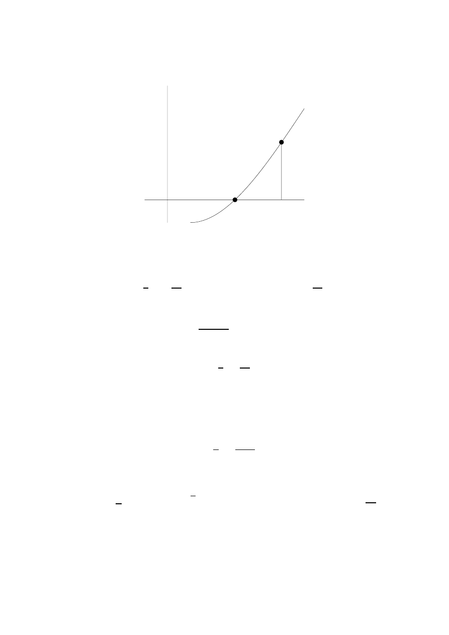
40
Chapter 4. Irrational Numbers
λ
p/q
f (p/q)
y = f (x)
Figure 2
and is nearer to λ than any other root of f (x) = 0, so that f (p/q)
6= 0.
Clearly (see Figure 2),
f
p
q
=
1
q
n
|a
0
p
n
+ a
1
p
n
−1
q +
· · · + a
n
q
n
| ≥
1
q
n
and
f (p/q)
λ
− p/q
< M
so that
λ −
p
q
>
c
q
n
and the theorem is proved.
Although Liouville’s theorem suffices for the construction of many transcen-
dental numbers, much interest centers on certain refinements. In particular, it
is desirable to have a theorem of the following type. If λ is of degree n then
λ −
p
q
<
M
q
f (n)
has at most a finite number of solutions. Here f (n) may be taken as n by
Liouville’s theorem . Can it be decreased? Thue, about 1990, first showed
that one could take f (n) =
n
2
and Siegel (1921) showed that we can take
f (n) = 2
√
n. This was slightly improved by Dyson and Schneider to
√
2n.
Very recently (1955), F. K. Roth created a sensation by proving that we can
take f (n) = 2 + ε. His proof is long and complicated. That we cannot take
f (n) = 2 (hence Roth’s result is in a way best possible) can be seen from the
following result due to Dirichlet.
Chapter 4. Irrational Numbers
41
For irrational λ there exist infinitely many solutions of
|λ −
p
q
| <
1
q
2
.
The proof is not difficult. Let λ be irrational and consider, for fixed n, the
numbers (λ), (2λ), . . . , (nλ), where (x) means “fractional part of x”. These n
points are distinct points on (0, 1); hence there exist two of them say iλ and
jλ whose distance apart is
≤
1
n
. Thus we have
(iλ)
− (jλ) <
1
n
or
kλ
− m ≤
1
n
(k and m integers
≤ n)
and
|λ −
m
k
| ≤
1
nk
≤
1
n
2
,
as required.
We now return to the application of Liouville’s theorem to the construction
of transcendental numbers.
Consider
1
10
1!
+
1
10
2!
+
· · · +
1
10
p!
= λ
p
as well as the real number λ = λ
∞
. It is easily checked that
|λ
∞
− λ
p
| <
1
λ
n+1
for every p. Hence λ is approximable to order n for any n and hence is not
algebraic.

Chapter 5
Congruences
In this section we shall develop some aspects of the theory of divisibility and
congruences.
If
a =
Y
p
α
and b =
Y
p
β
then it is easily seen that
(a, b) =
Y
p
min(α,β)
while [a, b] =
Y
p
max(α,β)
.
From these it follows easily that (a, b)
·[a, b] = a·b. We leave it as an exercise
to show that
(a, b) =
1
a
a
−1
X
α=1
a
−1
X
β=1
e
2πi
b
a
αβ
.
The notation a
≡ b (mod m) for m | (a−b) is due to Gauss. Rather obvious
properties of this congruence are a
≡ a, a ≡ b ⇒ b ≡ a, and a ≡ b and
b
≡ c ⇒ a ≡ c, i.e., ≡ is an equivalence relation. It is also easily proved that
a
≡ b and c ≡ d together imply ac ≡ bd; in particular a ≡ b ⇒ ka ≡ kb.
However the converse is not true in general. Thus 2
× 3 = 4 × 3 (mod 6) does
not imply 2
≡ 3 (mod 6). However, if (k, m) = 1 than ka ≡ kb does imply
a
≡ b.
Another important result is the following.
Theorem. If a
1
, a
2
, . . . , a
ϕ(m)
form a complete residue system mod m then
so does aa
1
, aa
2
, . . . , aa
ϕ(m)
provided (a, m) = 1.
Proof. We have ϕ(m) residues,. If two of them are congruent aa
i
≡ aa
j
, a(a
i
−
a
j
)
≡ 0. But (a, m) = 1 so that a
i
≡ a
j
.
An application of these ideas is to the important Euler’s theorem:
Theorem. If (a, m) = 1 then a
ϕ(m)
≡ 1 (mod m).
Proof. Since a
1
, a
2
, . . . , a
ϕ(m)
are congruent to aa
1
, aa
2
, . . . , aa
ϕ(m)
in some
order, their products are congruent. Hence
a
ϕ(m)
a
1
a
2
· · · a
ϕ(m)
≡ a
1
a
2
· · · a
ϕ(m)
44
Chapter 5. Congruences
and the result follows.
A special case of primary importance is the case m = p where we have
(a, p) = 1 =
⇒ a
p
−1
≡ 1 (mod p).
Multiplying by a we have for all cases a
p
≡ a (mod p). Another proof of this
result goes by induction on a; we have
(a + 1)
p
= a
p
+
p
1
a
p
−1
+
· · · + 1 ≡ a
p
≡ a (mod p).
One could also use the multinomial theorem and consider (1 + 1 +
· · · + 1)
p
.
Still another proof goes by considering the number of regular convex p-gons
where each edge can be colored in one of a colors. The number of such polygons
is a
p
, of which a are monochromatic. Hence a
p
− a are not monochromatic and
these come in sets of p each by rotation through
2πn
p
, n = 1, 2, . . . , p
− 1. The
idea behind this proof has considerable applicability and we shall return to at
least one other application a little later. We also leave as an exercise the task
of finding a similar proof of Euler’s theorem.
The theorems of Fermat and Euler may also be conveniently viewed from a
group-theoretic viewpoint. The integers relatively prime to m and < m form
a group under multiplication mod m. The main thing to check here is that
every element has an inverse in the system. If we seek an inverse for a we
form aa
1
, aa
2
, . . . , aa
ϕ(m)
. We have already seen that these are ϕ(m) numbers
incongruent mod m and relatively prime to m. Thus one of them must be the
unit and the result follows.
We now regain Euler’s proof from that of Lagrange’s which states that if a
is an element of a group G of order m, then a
m
= 1. In our case this means
a
ϕ(m)
≡ 1 or a
p
−1
≡ 1 if p is a prime.
The integers under p form a field with respect to + and
×. Many of the
important results of number theory are based on the fact that the multiplicative
part of this group (containing p
− 1 elements) is cyclic, i.e., there exists a
number g (called primitive root of p) such that 1 = g
0
, g
1
0, g
2
, . . . , g
p
−1
are
incongruent mod p. This fact is not trivial but we omit the proof. A more
general group-theoretic result in which it is contained states that every finite
field is automatically Abelian and its multiplicative group is cyclic.
In the ring of polynomials with coefficients in a field many of the theorems
of elementary theory of equations holds. For example if f (x) is a polynomial
whose elements are residue classes mod p then f (x)
≡ 0 (mod p) has at most
p solutions. Further if r is a root then x
− r is a factor. On the other hand, it
is not true that f (x)
≡ 0 (mod p) has at least one root.
Since x
p
− x ≡ 0 has at most p roots we have the factorization
x
p
− x ≡ x(x − 1)(x − 2) · · · (x − p + 1) (mod p)
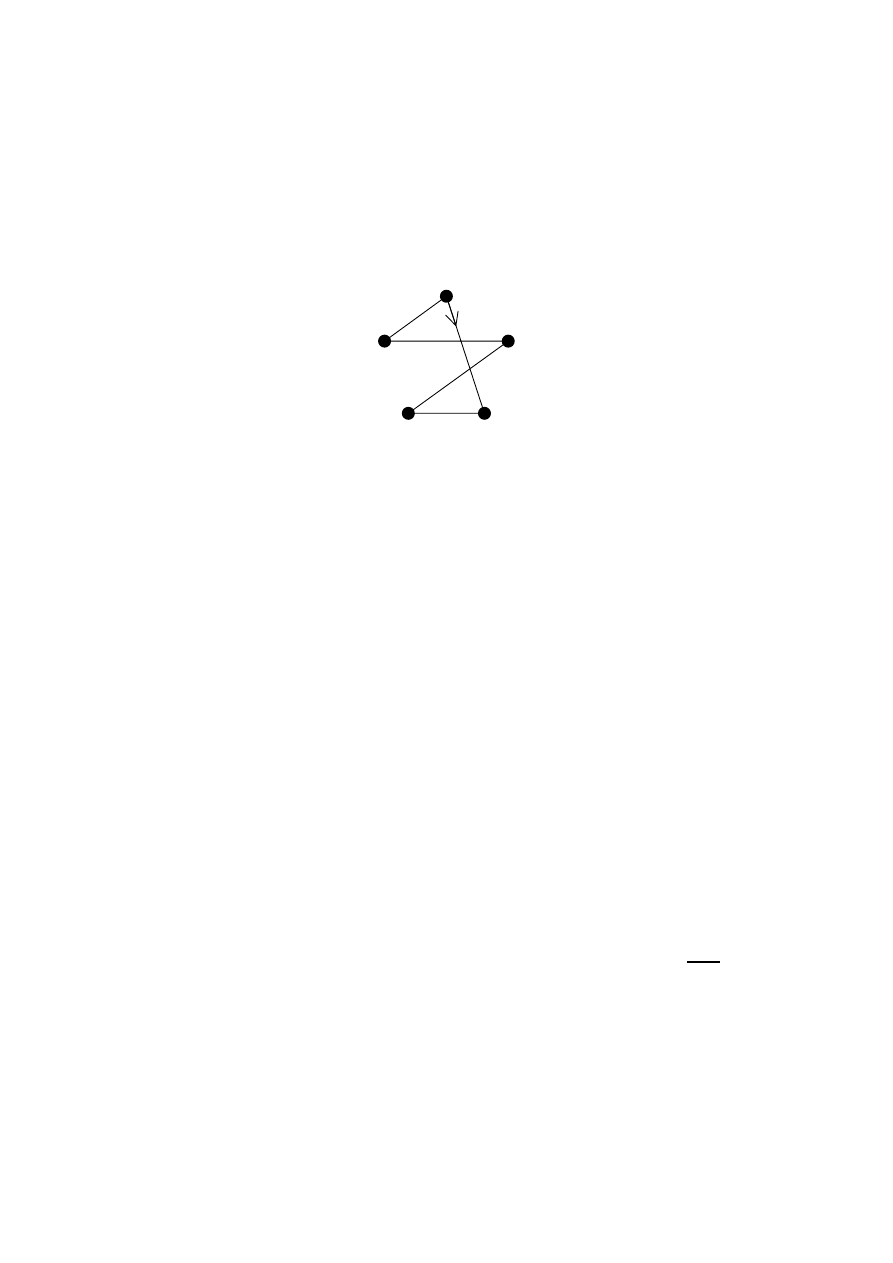
Chapter 5. Congruences
45
Comparing coefficients of x we have (p
− 1)! ≡ −1 (mod p) which is Wilson’s
theorem.
Cayley gave a geometrical proof of Wilson’s theorem as follows. Consider
the number of directed p-gons with vertices of a regular p-gon. (See Figure 3.)
Figure 3
These are (p
−1)! in number of which p−1 are regular. Hence the nonregular
ones are (p
− 1)! − (p − 1) in number and these come in sets of p by rotation.
Hence
(p
− 1)! − (p − 1) ≡ 0 (mod p)
and
(p
− 1)! + 1 ≡ 0 (mod p)
follows.
One can also give a geometrical proof which simultaneously yields both
Fermat’s and Wilson’s theorems and we suggest as a problem finding such a
proof.
Wilson’s theorem yields a necessary and sufficient condition for primality: p
is prime if and only if (p
− 1)! ≡ −1, but this is hardly a practical criterion.
Congruences with Given Roots
Let a
1
, a
2
, . . . , a
k
be a set of distinct residue classes (mod n). If there exists
a polynomial with integer coefficients such that f (x)
≡ 0 (mod m) has roots
a
1
, a
2
, . . . , a
k
and no others, we call this set compatible (mod n). Let the
number of compatible sets (mod n) be denoted by C(n). Since the number of
subsets of the set consisting of 0, 1, 2, . . . , n
− 1 is 2
n
, we call c(n) =
C(n)
2
n
the
coefficient of compatibility of n.
If n = p is a prime then the congruence
(x
− a
1
)(x
− a
2
)
· · · (x − a
k
)
≡ 0 (mod n)
has precisely the roots a
1
, a
2
, . . . , a
n
. Hence c(p) = 1. In a recent paper M.
M. Chokjnsacka Pnieswaka has shown that c(4) = 1 while c(n) < 1 for n =
46
Chapter 5. Congruences
6, 8, 9, 10. We shall prove that c(n) < 1 for every composite n
6= 4. We can
also prove that the average value of c(n) is zero, i.e.,
lim
n
→∞
1
n
(c(1) + c(2) +
· · · + c(n)) = 0.
Since c(n) = 1 for n = 1 and n = p we consider only the case where n is
composite. Suppose then that the unique prime factorization of n is given by
p
α
1
1
p
α
2
2
· · · with
p
α
1
1
> p
α
2
2
>
· · ·
Consider separately the cases
(1) n has more than one prime divisor, and
(2) n = p
α
, α > 1.
In case (1) we can write
n = a
· b, (a, b) = 1, a > b > 1.
We now show that if f (a)
≡ f(b) ≡ 0 then f(0) ≡ 0.
Proof. Let f (x) = c
0
+ c
1
+
· · · + c
m
x
m
. Then
0
≡ af(b) ≡ ac
0
(mod n) and
0
≡ bf(a) ≡ bc
0
(mod n).
Now since (a, b) = 1 there exist r, s, such that ar+bs = 1 so that c
0
(ar+bs)
≡ 0
and c
0
≡ 0.
In case (2) we can write
n = p
α
−1
p.
We show that f (p
α
−1
)
≡ 0 and f(0) ≡ 0 imply f(kp
α
−1
)
≡ 0, k = 2, 3, . . . .
Proof. Since f (0)
≡ 0, we have c
0
≡ 0,
f (x)
≡ c
1
+ c
2
x
2
+
· · · + c
m
x
m
, and
f (p
α
−1
)
≡ c
1
p
α
−1
≡ 0 (mod p
α
),
so that c
1
≡ 0 (mod p). But now f(kp
α
−1
)
≡ 0, as required.
On Relatively Prime Sequences Formed by Iterating
Polynomials (Lambek and Moser)
Bellman has recently posed the following problem. If p(x) is an irreducible
polynomial with integer coefficients and p(x) > x for x > c, prove that
{p
n
(c)
}
cannot be prime for all large n. We do not propose to solve this problem but
wish to make some remarks.

Chapter 5. Congruences
47
If p(x) is a polynomial with integer coefficients, then so is the k
th
iterate
defined recursively by p
0
(x) = x, p
k+1
(x) = p(p
k
(x)). If a and b are integers
then
p
k
(a)
≡ p
k
(b)
(mod (a
− b)).
(1)
In particular for a = p
n
(c) and b = 0 we have p
k+n
(c)
≡ p
k
(0) (mod p
n
(c)).
Hence
(p
k+n
(c), p
n
(c)) = (p
k
(0), p
n
(c)).
Hence
(p
k+n
(c), p
n
(c)) = (p
k
(0), p
n
(c)).
Hence
(p
k+n
(c), p
n
(c)) = (p
k
(0), p
n
(c)).
(2)
We shall call a sequence
{a
n
}, n ≥ 0, relatively prime if (a
m
, a
n
) = 1 for all
values of m, n, with m
6= n. From (2) we obtain
Theorem 1.
{p
n
(c)
}, n ≥ 0, is relatively prime if and only if (p
k
(0), p
n
(c)) =
1 for all k
≥ 0, n ≥ 0.
From this follows immediately a result of Bellman: If p
k
(0) = p(0)
6= 1 for
k
≥ 1 and if (a, p(0)) = 1 implies (p(a), p(0)) = 1 then {p
n
(a)
}, n ≥ a is
relatively prime whenever (c, p(0)) = 1.
We shall now construct all polynomials p(x) for which
{p
n
(c)
}, n ≥ 0, is
relatively prime for all c. According to Theorem 1,
{p
k
(0)
} = ±1 for all k ≥ 1,
as is easily seen by taking n = k and c = 0. But then
{p
k
(0)
} must be one of
the following six sequences:
1,
1,
1, . . .
1,
−1, 1, . . .
1,
−1, −1, . . .
−1, 1, 1, . . .
−1, 1, −1, . . .
−1, −1, 1, . . .
It is easily seen that the general solution of p(x) (with integer coefficients)
of m equations
p(a
k
) = a
k+1
,
k = 0, 1, 2, . . . , m
− 1,
is obtained from a particular solution p
1
(x) as follows.
p(x) = p
1
(x) + (x
− a
1
)(x
− a
2
)
· · · (x − a
k
−1
)
· Q(x),
(3)
where Q(x) is any polynomial with integer coefficients.
48
Chapter 5. Congruences
Theorem 2.
{p
n
(c)
}, n ≥ 0, is relatively prime for all c if and only if p(x)
belongs to one of the following six classes of polynomials.
1 + x(x
− 1) · Q(x)
1
− x − x
2
+ x(x
2
− 1) · Q(x)
1
− 2x
2
+ x(x
2
− 1) · Q(x))
2x
2
− 1 + x(x
2
− 1) · Q(x)
x
2
− x − 1 + x(x
2
− 1) · Q(x)
− 1 + x(x + 1) · Q(x)
Proof. In view of (3) we need only verify that the particular solutions yield
the six sequences given above.
On the Distribution of Quadratic Residues
A large segment of number theory can be characterized by considering it to be
the study of the first digit on the right of integers. Thus, a number is divisible
by n if its first digit is zero when the number is expressed in base n. Two
numbers are congruent (mod n) if their first digits are the same in base n. The
theory of quadratic residues is concerned with the first digits of the squares. Of
particular interest is the case where the base is a prime, and we shall restrict
ourselves to this case.
If one takes for example p = 7, then with congruences (mod 7) we have
1
2
≡ 1 ≡ 6
2
, 2
2
≡ 4 ≡ 5
2
, and 3
2
≡ 2 ≡ 4
2
; obviously, 0
2
≡ 0. Thus 1, 2, 4 are
squares and 3, 5, 6 are nonsquares or nonresidues. If a is a residue of p we write
a
p
= +1
while if a is a nonresidue we write
a
p
=
−1.
For p
| c we write
c
p
= 0. This notation is due to Legendre. For p = 7 the
sequence
a
p
is thus
+ +
− + − − .
For p = 23 it turns out to be
+ + + +
− + − + + − − + + − − + − + − − − − .
Chapter 5. Congruences
49
The situation is clarified if we again adopt the group theoretic point of view.
The residue classes (mod p) form a field, whose multiplicative group (containing
p
− 1 elements) is cyclic. If g is a generator of this group then the elements
may be written g
1
, g
2
, . . . , g
p
−1
= 1. The even powers of g are the quadratic
residues; they form a subgroup of index two. The odd powers of g are the
quadratic nonresidues. From this point of view it is clear
res
× res = res, res × nonres = nonres, nonres × nonres = res.
Further 1/a represents the unique inverse of a (mod p) and will be a residue
or nonresidue according as a itself is a residue or nonresidue.
The central theorem in the theory of quadratic residues and indeed one of
the most central results of number theory is the Law of Quadratic Reciprocity
first proved by Gauss about 1800. It states that
p
q
q
p
= (
−1)
(p
−1)(q−1)/4
.
It leads to an algorithm for deciding the value of
p
q
.
Over 50 proofs of this law have been given
1
including recent proofs by Zassen-
haus and by Lehmer. In Gauss’ first proof (he gave seven) he made use of the
following lemma—which he tells us he was only able to prove with considerable
difficulty. For p = 1 (mod 4) the least nonresidue of p does not exceed 2
√
p + 1.
The results we want to discuss today are in part improvements of this result
and more generally are concerned with the distribution of the sequence of +
and
− ’s in
a
p
, a = 1, 2, . . . , p
− 1.
In 1839 Dirichlet, as a by-product of his investigation of the class number
of quadratic forms, established the following theorem: If p
≡ 3 (mod 4) then
among the integers 1, 2, . . . ,
p
−1
2
, there are more residues than nonresidues.
Though this is an elementary statement about integers, all published proofs,
including recent ones given by Chung, Chowla, Whitman, Carlitz, and Moser
involve Fourier series. Landau was quite anxious to have an elementary proof.
Though somewhat related results have been given by Whitman and by Carlitz,
Dirichlet’s result is quite isolated. Thus, no similar nontrivial result is known
for other ranges.
In 1896 Aladow, in 1898 von Sterneck, and in 1906 Jacobsthall, took up
the question of how many times the combinations ++, +
−, −+, and −−
appear. They showed that each of the four possibilities appeared, as one might
expect, with frequency 1/4. In 1951 Perron examined the question again and
proved that similar results hold if, instead of consecutive integers, one considers
integers separated by a distance d. J. B. Kelly recently proved a result that,
1
Publisher’s note:
Over 200 proofs are now available.
50
Chapter 5. Congruences
roughly speaking, shows that the residues and non residues are characterized
by this property.
Jacobsthall also obtained partial results for the cases of
3 consecutive residues and non residues. Let R
n
and N
n
be the number of
blocks of n consecutive residues and non residues respectively.
One might
conjecture that R
n
∼ N
n
∼
p
2
n
. Among those who contributed to this question
are Vandiver, Bennet, Dorge, Hopf, Davenport, and A. Brauer. Perhaps the
most interesting result is that of A. Brauer. He showed that for p > p
0
(n),
R
n
> 0 and N
n
> 0. We shall sketch part of his proof. It depends on a very
interesting result of Van der Waerden (1927). Given k, `, there exists an integer
N = N (k, `) such that if one separates the integers 1, 2, . . . , N into k classes in
any manner whatsoever, at least one of the classes will contain an arithmetic
progression of length `. There are a number of unanswered questions about
this theorem to which we shall return in a later section.
Returning to Brauer’s work, we shall show he proves that all large primes
have, say, 7 consecutive residues. One separates the numbers 1, 2, . . . , p
−1 into
2 classes, residues and nonresidues. If p is large enough one of these classes will
contain, by Van der Waerden’s theorem, 49 terms in arithmetic progression,
say
a, a + b, a + 2b, . . . , a + 48b.
Now if
a
b
= c then we have 49 consecutive numbers of the same quadratic
character, namely
c, c + 1, c + 2, . . . , c + 48.
If these are residues we are done. If nonresidues then suppose d is the smallest
nonresidue of p. If d
≥ 7 we are finished for then 1, 2, . . . , 7 are consecutive
nonresidues. If d
≤ 7 consider the 7 nonresidues c, c + d, c + 2d, . . . , c + 6d. If
we now divide these by the nonresidue d we obtain 7 residues
c
d
,
c
d
+ 1, . . . ,
c
d
+ 6
and the result is complete.
The proof of the existence of nonresidues is considerably more complicated.
Furthermore it is interesting to note that the existence of block s like +
−+−· · ·
is not covered by these methods.
We now return to the question raised by Gauss. What can be said about
the least nonresidue n
p
of a prime? Since 1 is a residue, the corresponding
question about residues is “what is the smallest prime residue r
p
of p?”. These
questions were attacked in the 1920s by a number of mathematicians including
Nagel, Schur, Polya, Zeitz, Landau, Vandiver, Brauer, and Vinogradov. Nagel,
for example, proved that for p
6= 7, 23, n
p
<
√
p. Polya and Schur proved that
b
X
n=a
n
p
<
√
p log p.
Chapter 5. Congruences
51
This implies that there are never more than
√
p log p consecutive residues or
nonresidues and that ranges much larger than
√
p log p have about as many
residues as nonresidues. Using this result and some theorems on the distribu-
tion of primes, Vinogradov proved that for p > p
0
,
n
p
< p
1
2
√
e
log
2
p < p
.303
.
Checking through Vinogradov’s proof we found that by his method the p
0
is
excessively large, say p
0
> 10
10
10
. Nevertheless, in spite of numerous attempts
this result of Vinogradov has not been much improved.
In 1938 Erd˝
os and Ko showed that the existence of small nonresidues was
intimately connected with the nonexistence of the Euclidean Algorithm in qua-
dratic fields. This led Brauer, Hua, Min to re-examine the question of explicit
bounds for the least nonresidue. Brauer already in 1928 had proved a number
of such results, typical of which is that for all p
≡ 1 (mod 8),
n
p
< (2p)
.4
+ 3(2p)
.2
+ 1
and Hua and Min proved, for example, that for p > e
250
,
n
p
< (60
√
p)
.625
.
Small primes (under 10,000,000) were considered Bennet, Chatland, Brauer,
Moser and others.
Quite recently, the unproved extended Riemann hypothesis has been applied
to these problems by Linnik, Chowla, Erd˝
os, and Ankeny. Thus, for example,
Ankeny used the extended Riemann hypothesis to prove that n
p
6= O(log
2
p).
In the opposite direction Pillai (1945) proved that p
6= o(log log p). Using first
the Riemann hypothesis, and later some deep results of Linnik on primes in
arithmetic progression, Friedlander and Chowla improved this to n
p
6= o(log p).
Quite recently there have been a number of results in a somewhat different
direction by Brauer, Nagel, Skolem, Redei, and Kanold. Redei’s method is
particularly interesting. He uses a finite projective geometrical analogue of the
fundamental theorem of Minkowski on convex bodies to prove that for p
≡ 1
(mod 4), at least
1
7
of the numbers up to
√
p are residues and at least
1
7
are
non residues. Our own recent contributions to the theory are along these lines.
We shall outline some of this work.
Consider first the lattice of points in a square of side m. We seek an estimate
for V (m), the number of visible lattice points in the square. As on page 37 we
find
[m]
2
= V (m) + V
m
2
+
· · ·
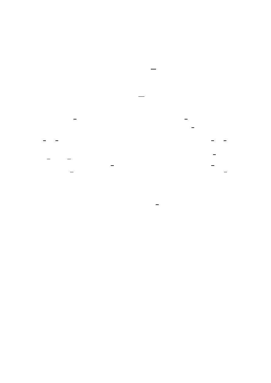
52
Chapter 5. Congruences
and inverting by the Mobius inversion formula yields
V (m) =
X
d
≥1
µ(d)
j
m
d
k
2
.
As before this leads to the asymptotic estimate
V (m)
∼
6
π
2
m
2
.
We can however obtain explicit estimates for v(m) also. Indeed, from the exact
formula for V (m) above one can show that for all m, V (m) > .6m
2
. We now
take m =
b√pc. For reasonably large p we shall have V (b√pc) > .59m
2
. Now
with each visible lattice point (a, b) we associate the number
a
b
(mod p). We
now show that distinct visible points correspond to distinct numbers. Thus if
a
b
=
c
d
then ad
≡ bc. But ad < p and bc < p. Hence ad = bc and
a
b
=
c
d
.
However (a, b) = (c, d) = 1 so that a = c and b = d.
Since we have at least .59 distinct numbers represented by fractions
a
b
, a <
√
p, b <
√
p, at least .09 of these will correspond to nonresidues. If R denotes
the number of residues <
√
p and N the number of nonresidues <
√
p, then
R + N =
√
p and 2RN > .09p. Solving these inequalities gives R, N > .04
√
p.
This is weaker than Nagel’s result but has the advantage of holding for primes
p
≡ 3 (mod 4) as well as p ≡ 1 (mod 4). Thus, exceptions turn out to be
only the primes 7 and 23. For primes p
≡ 1 (mod 4), −1 is a nonresidue and
this can be used together with above method to get stronger results. One can
also use the existence of many nonresidues <
√
p to prove the existence of one
small nonresidue, but the results obtainable in this way are not as strong as
Vinogradov’s result.
Chapter 6
Diophantine Equations
Volume 2 of Dickson’s History of the Theory of Numbers deals with Diophantine
equations. It is as large as the other two volumes combined. It is therefore
clear that we shall not cover much of this ground in this section. We shall
confine our attention to some problems which are interesting though not of
central importance.
One such problem is the Diophantine equation n! + 1 = x
2
mentioned in an
earlier section. The problem dates back to 1885 when H. Brochard conjectured
that the only solutions are 4!+1 = 5
2
, 5!+1 = 11
2
and 7!+1 = 71
2
. About 1895
Ramanujan made the same conjecture but no progress towards a solution of the
problem. About 1940 the problem appeared as an elementary (!!) problem in
the Monthly. No solutions were offered. However in 1950 an incorrect solution
was published and since that time several faulty attempts to prove the result
have been made. Again, about 1950 someone took the trouble to check, by
brute force, the conjecture up to n = 50. However, earlier, in his book on the
theory of numbers Kraitchik already had proved the result up to 5000. As far
as we know that is where the problems stands. We shall now give an indication
of Kraitchik’s method.
Suppose we want to check 100! + 1. Working (mod 103) we have
100!(
−2)(−1) ≡ −1, 100! +
1
2
≡ 0, 100! + 1 ≡
1
2
≡ 52.
If now 52 is a nonresidue of 103 we have achieved our goal. Otherwise we
could carry out a similar calculation with another p > 100, say 107. Note that
100! + 1
≡ 0 (mod 101) gives no information. Variations of this method can be
used to eliminate many numbers wholesale and this is what Kraitchik did. We
now outline a proof that
n! + 1 = x
8
has only a finite number of solutions. This proof depends on two facts which
we have not proved:
(1) Every odd prime divisor of x
2
+ 1 is of the form 4n + 1;
(2) There are roughly as many primes 4n + 1 as 4n + 3.
Now n! + 1 = x
8
gives n! = x
8
− 1 = (x
4
+ 1)(x
2
+ 1)(x
2
− 1); on the right
the contribution of primes 4k + 1 and 4k
−1 is about the same while on the left

54
Chapter 6. Diophantine Equations
all the odd prime factors of (x
4
+ 1)(x
2
+ 1) i.e., about (n!)
3/4
of the product,
are of the form 4n + 1.
We now go on to quite a different problem. Has the equation
1
n
+ 2
n
+
· · · + (m − 1)
n
= m
n
any solutions in integers other than 1 + 2 = 3? Here are some near solutions:
3
2
+ 4
2
= 5
2
,
3
3
+ 4
3
+ 5
3
= 6
3
,
1
6
+ 2
6
+ 4
6
+ 7
6
+ 9
6
+ 12
6
+ 13
6
+ 15
6
+ 16
6
+ 18
6
+ 20
6
+ 22
6
+ 23
6
= 28
6
.
We now outline a proof that if other solutions exist then m > 10
1000000
.
The rest of this section appeared originally as the paper “On the Diophantine
Equation 1
n
+ 2
n
+
· · · + (m − 1)
n
= m
n
,” Scripta Mathematica, 19 (1953),
pp. 84–88.
A number of isolated equations expressing the sum of the n
th
powers of
integers as an n
th
power of an integer have long been known. Some examples
are:
3
3
+ 4
3
+ 5
3
= 6
3
100
X
i=1
i
4
− 1
4
− 2
4
− 3
4
− 8
4
− 10
4
− 14
4
− 72
4
= 212
4
1
6
+ 2
6
+ 4
6
+ 5
6
+ 6
6
+ 7
6
+ 9
6
+ 12
6
+ 13
6
+ 15
6
+ 16
6
+ 18
6
+ 20
6
+ 21
6
+ 22
6
+ 23
6
= 28
6
.
Further examples and references to such results are given in [1, p. 682]. On the
other hand the only known solution in integers to the equation in the title is
the trivial one 1 + 2 = 3. In a letter to the author, P. Erd˝
os conjectured that
this is the only solution. The object of this note ts to show that if the equation
has a solution with n > 1, then m > 10
1000000
.
Let S
n
(m) denote
m
−1
X
i=1
i
n
. In what follows we assume
S
n
(m)
≡ m
n
,
n > 1.
(1)
It is possible to examine (1) with various moduli and thereby obtain restrictions
on m and n. This is essentially our method, but the moduli are so chosen that
we are able to combine the resulting congruences so as to obtain extremely
large bounds for m without laborious computation.
We use the following lemma.
Lemma 1. If p is a prime and ε
n
(p) is defined by ε
n
(p) =
−1 when (p−1) | n
and ε
n
(p) = 0 when (p
− 1) does not divide n then
S
n
(p)
≡ ε
n
(p)
(mod p).
(2)
Chapter 6. Diophantine Equations
55
A simple proof of (2) is given in [2, p. 90].
Now suppose p
| (m − 1), then
S
n
(m) =
m
−1
p
−1
X
i=0
p
X
j=1
(j + ip)
n
≡
m
− 1
p
· ε
n
(p)
(mod p).
On the other hand m
≡ 1 (mod p) so that by (1)
m
− 1
p
· ε
n
(p)
≡ 1 (mod p).
(3)
Hence ε
n
(p)
6≡ 0 (mod p) so that from the definition of ε
n
(p) it follows that
ε
n
(p) =
−1 and
p
| (m − 1) implies (p − 1) | n.
(4)
Thus (3) can be put in the form
m
− 1
p
+ 1
≡ 0 (mod p)
(5)
or
m
− 1 + p ≡ 0 (mod p
2
).
(6)
From (6) it follows that m
− 1 is squarefree. Further, since it is easily checked
that m
− 1 6= 2 it follows that m − 1 must have at least one prime divisor, so
by (4) n is even.
We now multiply together all congruences of the type (5), that is one for
each prime dividing m
− 1. Since m − 1 is squarefree, the resulting modulus is
m
− 1. Furthermore, products containing two or more distinct factors of the
form (m
− 1)/p will be divisible by m − 1. Thus we obtain
(m
− 1)
X
p
|(m−1)
1
p
+ 1
≡ 0 (mod m − 1)
(7)
or
X
p
|(m−1)
1
p
+
1
m
− 1
≡ 0 (mod 1).
(8)
The only values of m
≤ 1000 which satisfy (8) are 3, 7, 43.
We proceed to develop three more congruences, similar to (8), which when
combined with (8) lead to the main result. Equation (1) can be written in the
form
S
n
(m + 2) = 2m
n
+ (m + 1)
n
.
(9)
Suppose that p
| (m + 1). Using (2) and the fact that n is even, we obtain
as before
p
| (m + 1) implies (p − 1) | n
(10)
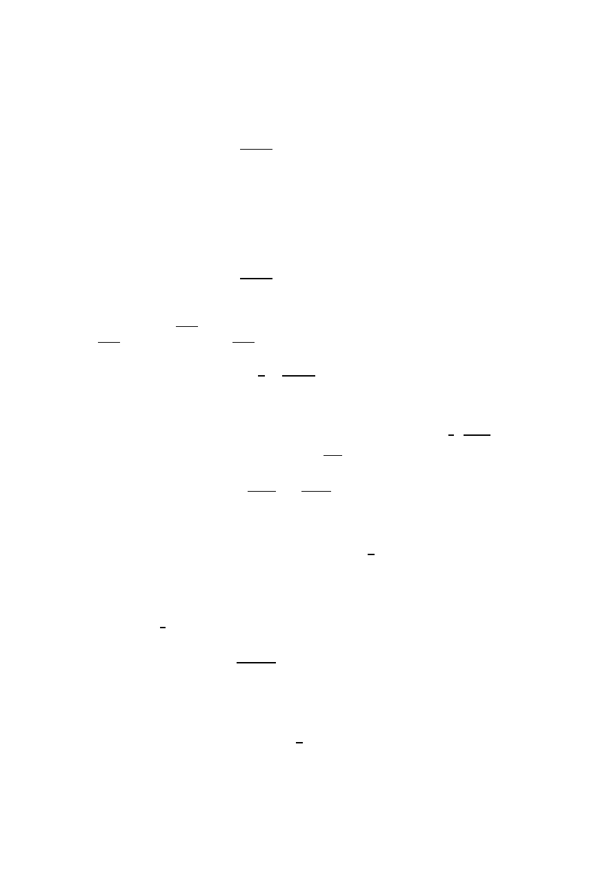
56
Chapter 6. Diophantine Equations
and
m + 1
p
+ 2
≡ 0 (mod p).
(11)
From (11) it follows that no odd prime appears with the exponent greater
than one in m + 1. The prime 2 however, requires special attention. If we
examine (1) with modulus 4, and we use the fact that n is even, then we find
that m + 1
≡ 1 or 4 (mod 8). Thus m + 1 is odd or contains 2 exactly to the
second power. If we assume the second of these possibilities then (11) can be
put in the form
m + 1
2p
+ 1
≡ 0 (mod p).
(12)
We multiply together all the congruences of the type (12). This modulus
then becomes
m+1
2
. Further, any term involving two or more distinct factors
m+1
2p
will be divisible by
m+1
2
so that on simplification we obtain
X
p
|(m+1)
1
p
+
2
m + 1
≡ 0 (mod 1).
(13)
We proceed to find two or more congruences similar to (13) without using the
assumption that m+1 is even. Suppose that p
| 2m−1 and let t =
1
2
2m
−1
p
−1
.
Clearly t is an integer and m
− 1 = tp +
p
−1
2
. Since n is even a
n
= (
−a)
n
so
that
S
n
p
− 1
2
≡
ε
n
(p)
2
(mod p).
Now
S
n
(m) =
t
−1
X
i=0
p
−1
X
j=1
(j + ip)
n
+
(p
−1)/2
X
i=1
i
n
≡
t +
1
2
ε
n
(p)
(mod p).
(14)
On the other hand m
n
≡ 0 (mod p) so that (1) and (14) imply ε
n
(p)
6≡ 0.
Hence p
− 1/n and by Fermat’s theorem m
n
≡ 1 (mod p). Thus (1) and (14)
yield
−
t+
1
2
≡ 1 (mod p). Replacing t by its value and simplifying we obtain
2m
− 1
p
+ 2
≡ 0 (mod p).
(15)
Since 2m
− 1 is odd (15) implies that 2m − 1 is squarefree. Multiplying
congruences of type (15), one for each of the r prime divisors of 2m
− 1 yields
2
r
−1
(2m
− 1)
X
p
|(2m−1)
1
p
+ 2
≡ 0 (mod 2m − 1).
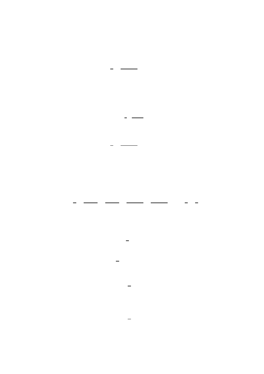
Chapter 6. Diophantine Equations
57
Since the modulus is odd this gives
X
p
|(2m−1)
1
p
+
2
2m
− 1
≡ 0 (mod 1).
(16)
Finally we obtain a corresponding congruence for primes dividing 2m + 1.
For this purpose we write (1) in the form
S
n
(m + 1) = 2m
n
.
(17)
Suppose p
| 2m + 1. Set v =
1
2
2m+1
p
− 1
. Using again an argument
similar to that employed to obtain (16) we find that (p
− 1) | n and 2m + 1 is
squarefree. Finally we obtain
X
p
|(2m+1)
1
p
+
4
2m + 1
≡ 0 (mod p).
(18)
We assume again that m + 1 is even so that (13) holds. If we now add the
left hand sides of (8), (13), (16), and (18) we get an integer, at least 4. No
prime p > 3 can divide more than one of the numbers m
− 1, m + 1, 2m − 1,
2m + 1. Further, 2 and 3 can divide st most two of these numbers. Hence if
M = (m
− 1)(m + 1)(2m − 1)(2m + 1) then
X
p
|M
1
p
+
1
m
− 1
+
2
m + 1
+
2
2m
− 1
+
4
2m + 1
≥ 4 −
1
2
−
1
3
.
(19)
We have already seen that the only possibilities for m with m
≤ 1000 are 3,
7, and 43. These are easily ruled out by (16). Thus (19) yields
X
p
|M
1
p
> 3.16.
(20)
From (20) it follows that if
X
p
≤x
1
p
< 3.16 then M >
Y
p
≤x
p. We shall prove the
following lemma.
Lemma 2.
X
p
≤10
7
1
p
< 3.16.
Proof. By direct computation
X
p
≤10
8
1
p
< 2.18.
(21)
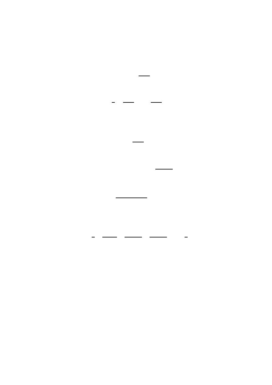
58
Chapter 6. Diophantine Equations
From Lehmer’s table [3] and explicit estimates for π(x) due to Rosser [4] it
can easily be checked that for 10
3
< x < 10
7
π(x) <
1.2x
log x
.
(22)
Now in [2, p. 339] it is shown that
X
p
≤x
1
p
=
π(x)
x
+
Z
x
2
π(x)
x
dx.
(23)
Combining (21), (22) and (23) gives the required result.
In [4] it is proved that
X
p
≤x
log p >
1
−
1
log x
x,
x < e
100
.
(24)
Hence
log M > log
Y
p
≤10
7
p =
X
p
≤10
7
log p >
1
−
1
7 log 10
10
7
> (.93)10
7
.
Now M < 4n
2
so that
log m >
log M
− log 4
2
> (.231)10
7
and m > e
(.231)10
7
> 10
1000000
.
Returning to the case m
− 1 odd, we note that in this we cannot use (13).
Letting N = (m
− 1)(2m − 1)(2m + 1) we get from (8), (16), and (18)
X
p
|N
1
p
+
1
m
− 1
+
2
2m
− 1
+
4
2m + 1
> 3
−
1
3
.
(25)
However, since the prime 2 does not appear on the left side (25) is actually
a stronger condition on m than is (19) so that in any case m > 10
1000000
.
References
[1] L.E. Dickson, History of the Theory of Numbers, vol. 2
[2] G. H. Hardy and E. M. Wright, An Introduction to the Theory of Num-
bers.
[3] D.H. Lehmer, “List of Prime Numbers from 1 to 10,006,721.”
[4] B. Rosser, “Explicit Bounds for Some Functions of Prime Numbers”,
Amer. Jour. of Math., 63 (1941), 211–232.
Chapter 7
Combinatorial Number Theory
There are many interesting questions that lie between number theory and com-
binatorial analysis. We consider first one that goes back to I. Schur (1917) and
is related in a surprising way to Fermat’s Last Theorem. Roughly speaking,
the theorem of Schur states that if n is fixed and sufficiently many consecu-
tive integers 1, 2, 3, . . . are separated into n classes, then at least one class will
contain elements a, b, c with a + b = c.
Consider the fact that if we separate the positive integers less than 2
n
into
n classes by putting 1 in class 1, the next 2 in class 2, the next 4 in class 3,
etc., then no class contains the sum of two of its elements. Alternatively, we
could write every integer m in form 2
k
θ where θ is odd, and place m in the kth
class. Again the numbers less than 2
n
will lie in n classes and if m
1
= 2
k
θ
1
and
m
2
= 2
k
θ
2
are in class k then m
1
+ m
2
= 2
k
(θ
1
+ θ
2
) lies in a higher numbered
class. The more complicated manner of distributing integers outlined below
enables us to distribute 1, 2, . . . ,
3
n
−1
2
into n classes in such a way that no class
has a solution to a + b = c:
1
2
5
3
4
6
10
11
7
13
12
8
..
.
..
.
..
.
On the other hand, the theorem of Schur states that if one separates the
numbers 1, 2, 3, . . . , [n! e] into n classes in any manner whatsoever then at least
one class will contain a solution to a + b = c. The gap between the last two
statements reveals an interesting unsolved problem, namely, can one replace
the [n! e] in Schur’s result by a considerably smaller number? The first two
examples given show that we certainly cannot go as low as 2
n
− 1, and the last
example shows that we cannot go as low as
3
n
−1
2
.
We now give a definition and make several remarks to facilitate the proof of
Schur’s theorem.
Let T
0
= 1, T
n
= nT
n
−1
+ 1. It is easily checked that
T
n
= n!
1 +
1
1!
+
1
2!
+
· · · +
1
n!
= [n! e].
60
Chapter 7. Combinatorial Number Theory
Thus Schur’s theorem can be restated as follows: If 1, 2, . . . , T
n
are separated
into n classes in any manner whatever, at least one class will contain a solution
of a + b = c. We will prove this by assuming that the numbers 1, 2, . . . , T
n
have
been classified n ways with no class containing a solution of a + b = c and from
this obtain a contradiction. Note that the condition a + b
6= c means that no
class can contain the difference of two of its elements.
Suppose that some class, say A, contains elements a
1
< a
2
<
· · · . We form
differences of these in the following manner:
b
1
= a
2
− a
1
, b
2
= a
3
− a
1
, b
3
= a
4
− a
1
, . . .
c
1
= b
2
− b
1
, c
2
= b
3
− b
1
, c
3
= b
4
− b
1
, . . .
d
1
= c
2
− c
1
, d
2
= c
3
− c
1
, d
3
= c
4
− c
1
, . . .
and so on. We note that all the b’s, c’s, d’s, etc., are differences of a’s and
hence cannot lie in A.
Now, we start with T
n
elements. At least
T
n
n
+ 1
= T
n
−1
+ 1
of these must lie in a single class, say A
1
. We then form T
n
−1
b’s. These do
not lie in A
1
and hence lie in the remaining n
− 1 classes. At least
T
n
−1
n
− 1
+ 1
= T
n
−2
+ 1
of them must lie in a single class, say A
2
. Form their T
n
−2
differences, the c’s.
These yield T
n
−2
numbers neither in A
1
nor A
2
. Continuing in this manner
yields T
n
−3
numbers not in A
1
, A
2
, A
3
. In this manner we eventually obtain
T
0
= 1 number not belonging to A
1
, A
2
, . . . , A
n
. But all numbers formed are
among the numbers 1, 2, . . . , T
n
so we have a contradiction, which proves the
theorem.
We state, without proof, the connection with Fermat’s last theorem. A
natural approach to Fermat’s theorem would be to try to show that x
n
+y
n
= z
n
(mod p) is insolvable modulo some p, provided p does not divide x
· y · z.
However, Schur’s theorem can be used to show that this method must fail and
indeed if p > n! e then x
n
+ y
n
= z
n
(mod p) has a solution with p not a factor
of xyz.
Somewhat related to Schur’s theorem is a famous theorem of Van der Waer-
den, which we briefly investigate. In the early 1920’s the following problem
arose in connection with the theory of distribution of quadratic residues. Imag-
ine the set of all integers to be divided in any manner into two classes. Can
one assert that arithmetic progressions of arbitrary length can be found is at
least one of these classes? The problem remained unsolved for several years
in spite of concentrated efforts by many outstanding mathematicians. It was
Chapter 7. Combinatorial Number Theory
61
finally solved in 1928 by Van der Waerden. As is not uncommon with such
problems, Van der Waerden’s first step was to make the problem more general,
and hence easier.
Van der Waerden proved the following: Given integers k and `, there exists
an integer W = W (k, `) such that if the numbers 1, 2, 3, . . . , W are separated
into k classes in any manner, then at least one class will contain ` terms in
arithmetic progression. We will not give Van der Waerden’s proof here. It is
extremely tricky, difficult to see through, and leads only to fantastically large
bound for W (k, `). For this reason the reader might consider the very worth-
while unsolved problem of finding an alternative simpler proof that W (k, `)
exists and finding reasonable bounds for it. We will have a little more to say
about the function W (k, `) a little later.
Our next problem of combinatorial number theory deals with “nonaverag-
ing” sequences. We call a sequence A : a
1
< a
2
< a
3
<
· · · non-averaging if it
does not contain the average of two of its elements, i.e., a
i
+ a
j
6= 2a
k
(i
6= j).
Let A(n) denote the number of elements in A not exceeding n. The main
problem is to estimate how large A(n) can be if A is nonaveraging. We can
form a nonaveraging sequence by starting with 1, 2, . . . and then always taking
the smallest number that does not violate the condition for nonaveraging sets.
In this way we obtain 1, 2, 4, 5, 10, 11, 13, 14, 28, 29, 31, . . . . It is an interesting
fact that this sequence is related to the famous Cantor ternary set. Indeed, we
leave it as an exercise to prove that this sequence can be obtained by adding 1
to each integer whose representation in base 3 contains only 0’s and 1’s . This
sequence is maximal in the sense that no new number can be inserted into the
sequence without destroying its nonaveraging character. This, as well as other
facts, led Szekeres (about 1930) to conjecture that this set was as dense as any
nonaveraging set. For this set, the counting function can easily be estimated
to be
∼ n
log 2/ log 3
. It therefore came as a considerable surprise when Salem
and Spencer (1942) proved that one could have a nonaveraging set of integers
≤ n containing at least n
1
−c/
√
log log n
elements.
Given a number x, written in base ten, we decide whether x is in R on the
basis of the following rules.
First we enclose x in a set of brackets, putting the first digit (counting from
right to left) in the first bracket, the next two in the second bracket, the next
three in the third bracket, and so on. If the last nonempty bracket (the bracket
furthest to the left that does not consist entirely of zeros) does not have a
maximal number of digits, we fill it with zeros. For instance, the numbers
a = 32653200200,
b = 100026000150600,
c = 1000866600290500
would be bracketed
a = (00003)(2653)(200)(20)(0),
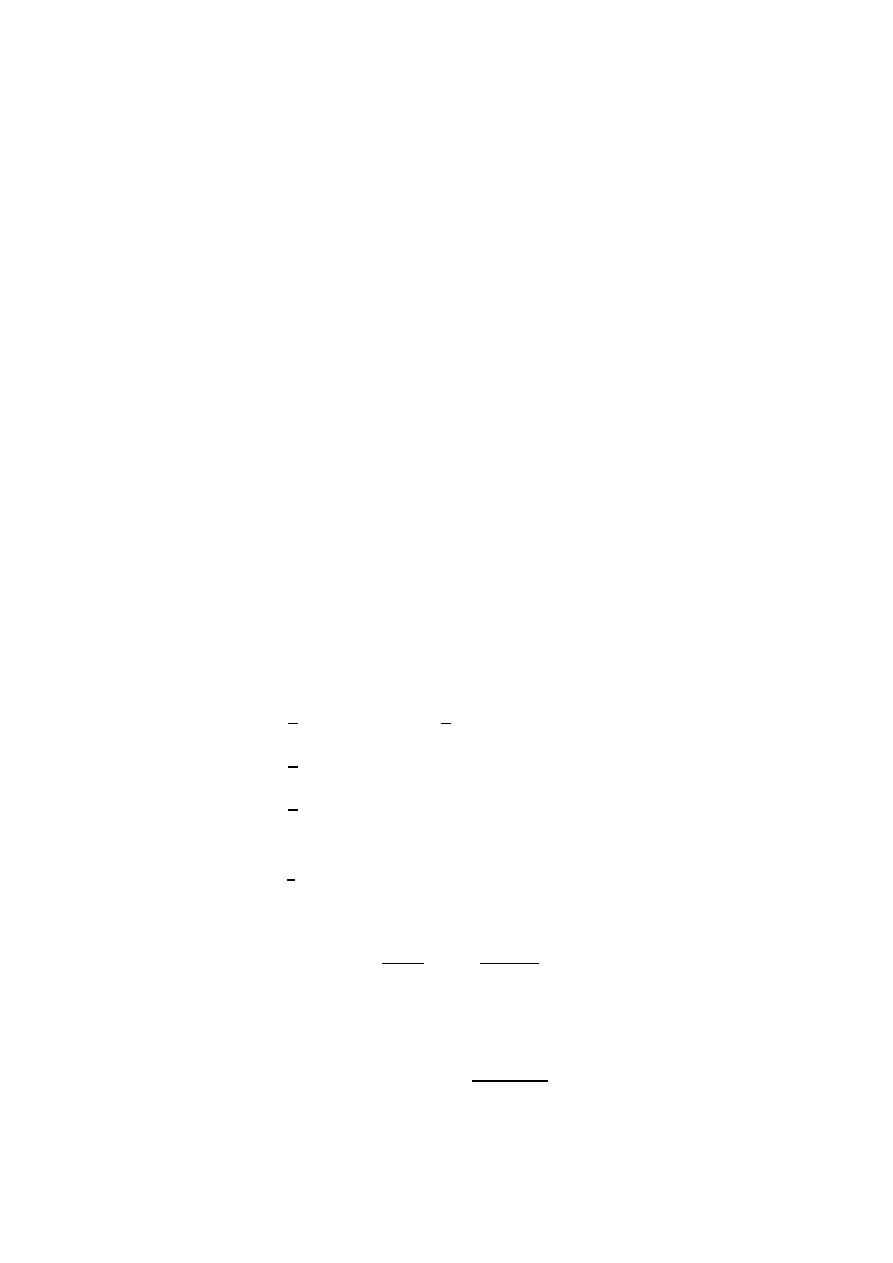
62
Chapter 7. Combinatorial Number Theory
b = (10002)(6100)(150)(60)(0),
c = (10008)(6600)(290)(50)(0),
respectively. Now suppose the r
th
bracket in x contains nonzero digits, but all
further brackets to the left are 0. Call the number represented by the digits
in the i
th
bracket x
i
, i = 1, 2, . . . , r
− 2. Further, denote by ¯x the number
represented by the digit in the last two brackets taken together, but excluding
the last digit. For x to belong to R we require
(1) the last digit of x must be 1,
(2) x
i
must begin with 0 for i = 1, 2, . . . , r
− 2,
(3) x
2
1
+
· · · + x
2
r
−2
= ¯
x.
In particular, note that a satisfies (2) but violates (1) and (3) so that a is not
in R; but b and c satisfy all three conditions and are in R. To check (3) we
note that 60
2
+ 150
2
= 26100.
We next prove that no three integers in R are in arithmetic progression.
First note that if two elements of R have a different number of nonempty
brackets their average cannot satisfy (1). Thus we need only consider averages
of elements of R having the same number of nonempty brackets. From (1) and
(3) it follows that the two elements of R can be averaged bracket by bracket
for the first r
− 2 brackets and also for the last two brackets taken together.
Thus, in our example,
1
2
(60 + 50) = 55,
1
2
(150 + 290) = 220,
1
2
(100026100 + 100086600) = 100056350,
1
2
(b + c) = (10005)(6350)(220)(55)(0)
This violates (3) and so is not in R. In general we will prove that if x and y
are in R then ¯
z =
1
2
(x + y) violates (3) and so is not in R.
Since x and y are in R,
¯
z =
¯
x + ¯
y
2
=
r
−2
X
i=1
x
2
i
+ y
2
i
2
.
On the other hand, z in R implies
¯
z =
r
−2
X
i=1
z
2
i
=
r
−2
X
i=1
(x
i
+ y
i
)
2
2
.
Chapter 7. Combinatorial Number Theory
63
Hence, if z is in R then
r
−2
X
i=1
x
2
i
+ y
2
i
2
=
r
−2
X
i=1
(x
i
+ y
i
)
2
2
.
Thus
r
−2
X
i=1
(x
i
− y
i
)
2
2
= 0,
which implies x
i
= y
i
for i = 1, 2, . . . , r
− 2. This together with (1) and (2)
implies that x and y are not distinct.
Szekeres’ sequence starts with 1, 2, 4, 5, 10, 11, . . . . Our sequence starts with
100000, 1000100100, 1000400200, . . . .
Nevertheless, the terms of this sequence are eventually much smaller than the
corresponding terms of Szekeres’ sequence. We now estimate how many integers
in R contain exactly r brackets. Given r brackets we can make the first digit
in each of the r
− 2 brackets 0. We can fill up the first r − 2 brackets in as
arbitrary manner. This can be done in
10
0+1+2+
···+(r−2)
= 10
1
2
(r
−1)(r−2)
ways. The last two brackets can be filled in such a way as to satisfy (1) and
(3).
To see this we need only check that the last two brackets will not be overfilled,
and that the last digit, which we shall set equal to 1, will not be interfered with.
This follows from the inequality
(10
1
)
2
+ (10
2
)
2
+
· · · + (10
r
−2
)
2
< 10
2(r
−1)
.
For a given n let r be the integer determined by
10
1
2
r(r+1)
≤ n < 10
1
2
(r+1)(r+2)
.
(4)
Since all the integers with at most r brackets will not exceed n, and since r
brackets can be filled to specification in 10
1
2
(r
−2)(r−1)
ways, we have
R(n)
≥ 10
1
2
(r
−1)(r−2)
.
(5)
From the right hand side of (4) we have
r + 2 >
p
2 log n
so that (5) implies that
R(n)
≥ 10
1
2
(r
−1)(r−2)
> 10
log n
−c
√
log n
> 10
(log n)
(
1
−c/
√
log n
)
where all logs are to base 10.
64
Chapter 7. Combinatorial Number Theory
An old conjecture was that
A(n)
n
→ 0 for every nonaveraging sequence. This
has only been proved quite recently (1954) by K. F. Roth. His proof is not
elementary.
L. Moser has used a similar technique to get lower bounds for the Van der
Waerden function W (k, `). He proved that W (k, `) > `k
log k
, i.e., he showed
how to distribute the numbers 1, 2, . . . , [`k
log k
] into k classes in such a way
that no class contains 3 terms in arithmetic progression. Using a quite different
method Erd˝
os and Rado have shown that W (k, `) >
√
2`k
`
.
Erd˝
os has raised the following question: What is the maximum number of
integers a
1
< a
2
<
· · · < a
k
≤ n such that the 2
k
sums of distinct a’s are all
distinct? The powers of 2 show that one can give k + 1 a’s not exceeding 2
k
and one can in fact give k + 2 a’s under 2
k
satisfying the required condition.
On the other hand, all the sums involved are less than kn so that
2
k
≤ kn,
(1)
which implies
k <
log n
log 2
+ (1 + o(1))
log log n
log 2
.
(2)
We now show how Erd˝
os and Moser improved these estimates to
2
k
< 4
√
kn,
(3)
which implies
k <
log n
log 2
+ (1 + o(1))
log log n
2 log 2
.
(4)
The conjecture of Erd˝
os is that
k =
log n
log 2
+ o(1).
(5)
Denote the sum of distinct a’s by s
1
, s
2
, . . . , s
2
k
and let A = a
1
+a
2
+
· · ·+a
k
.
Observe that the average sum is
A
2
since we can pair each sum with the sum
of the complementary set. This suggests that we estimate
P
i
s
i
−
A
2
2
.
We have
X
i
s
i
−
A
2
2
=
X 1
2
(
±a
1
± a
2
± · · · ± a
k
)
2
,
where the last sum runs over the 2
k
possible distributions of sign. Upon squar-
ing we find that all the cross terms come in pairs while each a
2
i
will appear 2
k
times. Thus
X
i
s
i
−
A
2
2
= 2
k
X
a
2
i
< 2
k
−2
n
2
k.
Chapter 7. Combinatorial Number Theory
65
Thus the number of sums s
i
for which
s
i
−
A
2
≥ n
√
k
cannot exceed 2
k
−1
. Since all the sums are different, we have 2
k
−1
distinct
numbers in a range of length 2n
√
k. This yields 2
k
−1
≤ 2n
√
k as required.
Let a
1
< a
2
< . . . be an infinite sequence of integers and define f (n) to be
the number of solutions of n = a
i
+ a
j
where all solutions count once. G. A.
Dirac and D. J. Newman gave the following interesting proof that f (n) cannot
be constant from some stage on. If f (` + 1) = f (` + 2) =
· · · we would have
1
2
X
z
a
k
2
+
X
z
2a
k
=
X
f (n)z
n
= P
`
(z) + a
z
`+1
1
− z
,
(f (` + 1) = a),
where P (z) is a polynomial of degree
≤ `. If z → −1 on the real axis the right
side remains bounded, but the left side approaches infinity, since both terms on
the left side are positive, and the second tends to infinity. This contradiction
proves the theorem.
Turan and and Erd˝
os conjectured that if f (n) > 0 for all sufficiently large n
then lim sup f (n) =
∞ but this seems very difficult to prove. A still stronger
conjecture would be that if a
k
> ck
2
then lim sup f (n) =
∞. The best known
result in this direction is only lim sup f (n)
≥ 2.
Fuchs and Erd˝
os recently proved that
n
X
k=1
f (k) = cn + o
n
1
4
log n
!
is impossible. If a
k
= k
2
one comes to the problem of lattice points in a circle
of radius n. Here Hardy and Landau proved
n
X
k=1
f (k) = πn + o(n log n)
does not hold. Though not quite as strong as this, the result of Erd˝
os and
Fuchs is applicable to a much more general situation and is much easier (but
not very easy) to prove.
Let a
1
< a
2
<
· · · be an infinite sequence of integers. Erd˝os conjectured,
and G. G. Lorentz proved, that there exists a sequence
{b
i
} of zero density
such that every integer is of the form a
i
+ b
j
.
An interesting unsolved problem along these lines is to find a sequence B :
b
1
< b
2
<
· · · with counting function B(n) <
cn
log n
such that every integer is of
the form 2
k
+ b
j
.
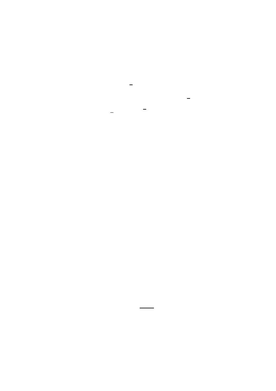
66
Chapter 7. Combinatorial Number Theory
Let a
1
< a
2
<
· · · < a
2n
be 2n integers in the interval [1, 4n] and b
1
<
b
2
<
· · · < b
2n
the remaining numbers in the interval. Erd˝
os conjectured that
there exists an integer x such that the number of solutions of a
i
+ x = b
j
is at
least n. It is quite easy to show that there exists an x so that the number of
solutions of a
i
+ x = b
j
is at least
n
2
. We merely observe that the number of
solutions of a
i
+ y = b
j
is 4n
2
and that there are 8n possible choices of y, i.e.,
−4n ≤ y ≤ 4n, y 6= 0. Thus for some y
0
there are at least
n
2
b’s in a
i
+ y
0
as
stated.
P. Scherk improved the
n
2
to n(2
−
√
2) = .586n. By an entirely different
method L. Moser improved this further to .712n. On the other hand Selfridge,
Ralston and Motzkin have used S.W.A.C. to disprove the original conjecture
and have found examples where no number is representable more than .8n
times as a difference between an a and a b.
Still another set of interesting problems of combinatorial number theory re-
volve about the concept of addition chain introduced by A. Scholz. An addition
chain for n is a set of integers 1 = a
0
< a
1
<
· · · < a
r
= n such that every
element a
p
can be written as a sum a
σ
+ a
τ
of preceding elements of the chain.
For example for n = 666
1, 2, 4, 8, 16, 24, 40, 80, 160, 320, 640, 664, 666
form a chain with r = 12; the same holds for
1, 2, 3, 6, 9, 18, 27, 54, 81, 162, 324, 648, 666.
In any case we must have a
1
= 2, and a
2
= 3 or 4. By the length ` = `(n)
Scholtz understands the smallest ` for which there exists an addition chain
a
0
, a
1
, . . . , a
`
= n.
Scholtz stated the following:
m + 1
≤ `(n) ≤ 2m for 2
m
+ 1
≤ n ≤ 2
m+1
(m
≥ 1);
`(ab)
≤ `(a) + `(b);
`(2
m+1
− 1) ≤ m + `(m + 1).
The first two of these are easy to prove. The third we would conjecture
to be false. Scholtz surmised that the first could be improved and raised the
question of whether or not
1
≤ lim sup
n
→∞
`(n)
log
2
n
≤ 2
could be improved.
In what follows we prove (1) and outline a proof due to A. Brauer that
`(n)
∼ log
2
n.
Chapter 7. Combinatorial Number Theory
67
Suppose integers are written in base 2 and we seek an addition chain for
10110110 say. We might form the chain
1, 10, 100, 101, 1010, 1011, 10110, 101100, 101101, 1011010,
1011011, 10110110, 101101100, 101101101.
In this process, each digit “costs” at most two elements in the chain so that
` < 2 log
2
n. Since the left hand side of the inequality of (1) is trivial the
method suggested above yields a proof of (1).
Brauer’s idea is to build up a large stock of numbers first and use it when
the occasion arises. Suppose n is about 2
m
. We start out with the chain
1, 2, . . . , 2
r
, where r will be determined later. We can now break up the digits
of n into m/r blocks with r digits in each block. For example, suppose
n = (101)(110)(010)(101)(111)
Here m = 15, r = 3.
Starting with our stock of all 3 digit numbers we can proceed as follows:
1, 10, 100, 101, 1010, 10100, 101000, 101110,
1011100, 10111000, 101110000, 101110010, . . .
where between the underlined stages we double and at the underlined stages
we add the appropriate number from our stock to build up n. In this case we
would need 2
3
+ 2
15
+ 5 steps. In general, the number of steps for a number
under 2
m
would be about 2
r
+ m +
m
r
. By appropriate choice of r we could
make 2
r
+
m
r
as small as we please in comparison with m. Indeed, using this
idea Brauer proved in general
`(n) < log
2
n
1 +
1
log log n
+
2 log 2
(log n)
1
−log 2
.

Chapter 8
Geometry of Numbers
We have already seen that geometrical concepts are sometimes useful in illumi-
nating number theoretic considerations. With the introduction by Minkowski
of geometry of numbers a real welding of important parts of number theory and
geometry was achieved. This branch of mathematics has been in considerable
vogue in the last 20 years, particularly in England where it was and is being
developed vigorously by Mordell, Davenport, Mahler and their students.
We shall consider a very brief introduction to this subject. First, we shall
examine a proof of the fundamental theorem of Minkowski due to Hajos (1934),
then we shall discuss some generalizations and applications of this theorem, and
finally we shall investigate some new results and conjectures that are closely
related.
In its simplest form the fundamental theorem of Minkowski is the following.
Let R be a region in the x-y plane of area A > 4, symmetric about the origin
and convex. Then R contains a lattice point other than the origin.
First, some preliminary remarks. In the condition A > 4, the 4 cannot be
replaced by any smaller number. This may be seen by considering the square
of side 2
− ε, centered at the origin. Indeed this example might at first suggest
that the theorem is quite intuitive, as it might seem that squeezing this region
in any direction and keeping its area fixed would necessarily force the region to
cover some lattice point. However the matter is not quite so simple, as other
examples reveal that neither central symmetry nor convexity are indispensable.
As far as convexity is concerned what is really needed is that with the vectors
−
→
V
1
and
−
→
V
2
the region should also contain
1
2
(
−
→
V
1
+
−
→
V
2
). The symmetry means
that with
−
→
V
1
the vector
−
−
→
V
1
should also be in R. Thus the symmetry and
convexity together imply that, if
−
→
V
1
and
−
→
V
2
are in R, so is
1
2
(
−
→
V
1
−
−
→
V
2
). This
last condition is really sufficient for our purpose and may replace the conditions
of symmetry and convexity. It is implied by symmetry and convexity but does
not imply either of these conditions.
Another example that perhaps illuminates the significance of Minkowski’s
theorem is the following. Consider a line through O having irrational slope
tan θ; see Figure 4. This line passes through no lattice point other than the
origin. If we take a long segment of this line, say extending length R on either
side of O, then there will be a lattice point closest to, and a distance r from,
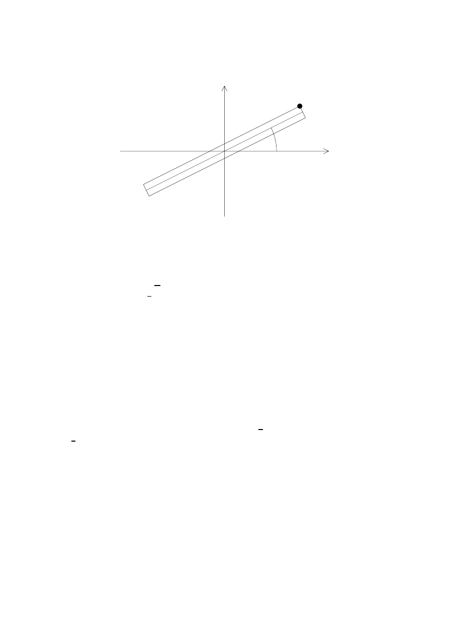
70
Chapter 8. Geometry of Numbers
θ
(p, q)
Figure 4.
The long side of the rectangle is 2R, the short 2r.
this segment. Hence, no matter how large R is, we can construct a rectangle
containing this line segment, which contains no lattice point other than O. By
the fundamental theorem of Minkowski the area 4rR of this rectangle does not
exceed 4. Thus r
≤
1
R
. Note that if (p, q) is a lattice point on the border of
the rectangle then
p
q
≈ tan θ, so that the fundamental theorem of Minkowski
will give some information about how closely an irrational number can be
approximated by rationals.
Let us now return to Hajos proof of the fundamental theorem of Minkowski.
Consider the x-y plane cut up into an infinite chessboard with the basic square
of area 4 determined by
|x| ≤ 1, |y| ≤ 1. We now cut up the chessboard along
the edges of the squares and superimpose all the squares that contain parts
of the region R. We have now compressed an area > 4 into a region of area
4. This implies that there will be some overlapping, i.e., one can stick a pin
through the square so as to pierce R into two points say V
1
and V
2
. Now
reassemble the region and let the points V
1
and V
2
be the vectors
−
→
V
1
and
−
→
V
2
.
Consider the fact that the x and y coordinates of V
1
and V
2
differ by a multiple
of 2. We write V
1
≡ V
2
(mod 2), which implies
1
2
(V
1
− V
2
)
≡ 0 (mod 1). Thus
1
2
(V
1
− V
2
) is a lattice point different from O (since V
1
6= V
2
) in R.
The fundamental theorem of Minkowski can easily be generalized to n-
dimensional space. Indeed we need only replace 4 in the fundamental theorem
of Minkowski by 2
n
and Hajos’ proof goes through. Many extensions and re-
finements of the fundamental theorem of Minkowski have been given. I shall
return to some of them later.
One of Polya’s earliest papers has the long and curious title “Zahlhlenthe-
oretisches und Wahrscheinlichkeitstheoretisches ¨
uber die Sichtweite in Walde
und durch Schneefall”. A proof of Polya’s main result in this paper can be
greatly simplified and somewhat refined using the fundamental theorem of
Minkowski. The problem is this.
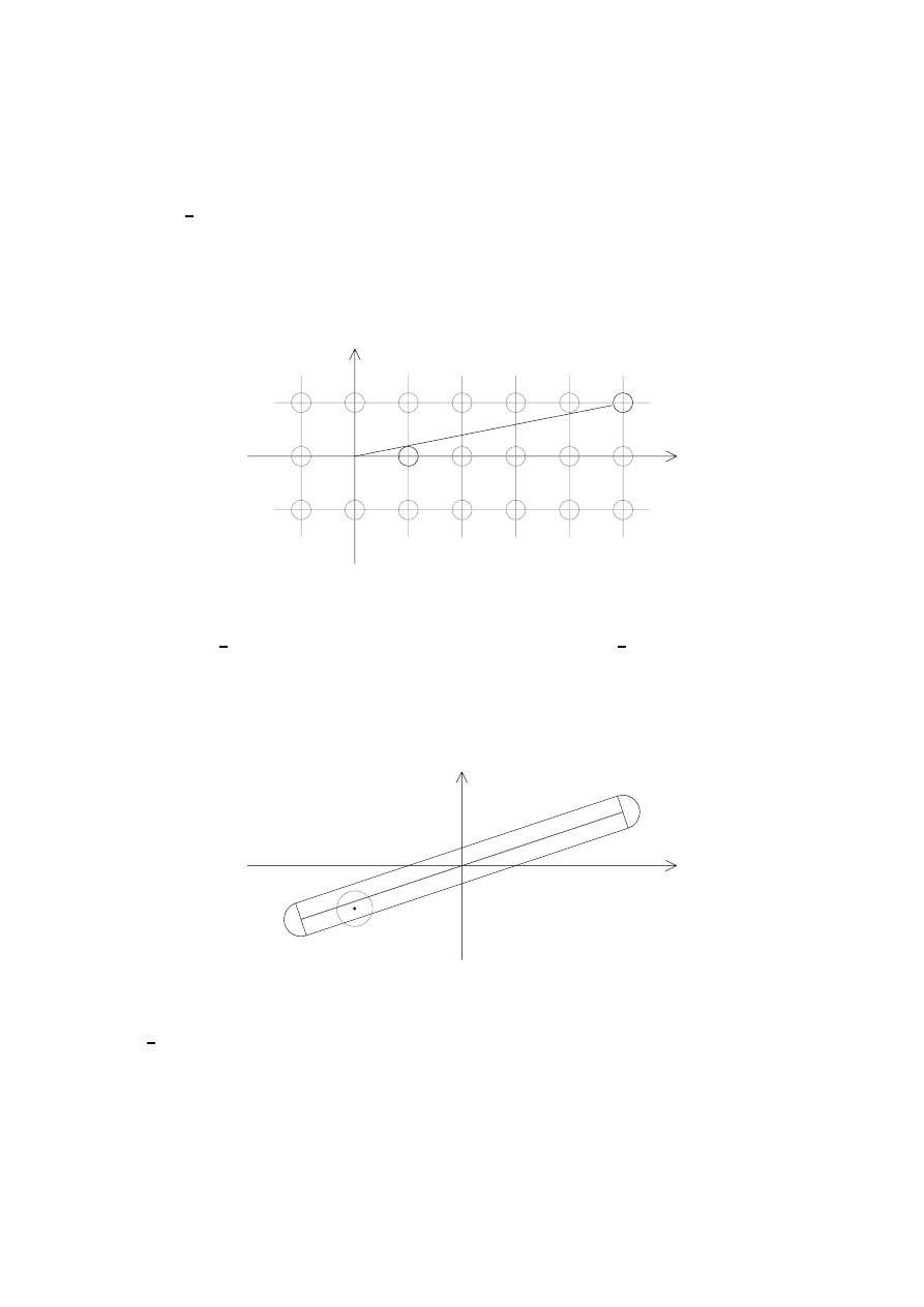
Chapter 8. Geometry of Numbers
71
Suppose every lattice point other than O is surrounded by a circle of radius
r
≤
1
2
(a tree in a forest). A man stands at O. In direction θ he can see a
distance f (r, θ). What is the furthest he can see in any direction? That is,
determine
F (r) = max
θ
f (θ, r).
O
Figure 5
By looking past the circle centered at (1, 0) (Figure 5), we can see almost a
distance
1
r
. On the other hand we can prove that F (r)
≤
1
r
. For suppose that
we can see a distance F (r) in direction θ. About this line of vision construct a
rectangle with side 2r. This rectangle contains no lattice point, for otherwise
the tree centered at such a lattice point would obstruct our line of vision; see
Figure 6.
Figure 6
Hence, by the fundamental theorem of Minkowski 4F (r)r
≤ 4 and F (r) ≤
1
r
as required. Note that no lattice point can be in either semicircle in the
diagram. This enables us to improve slightly on Polya’s result. I shall leave
the details as an exercise.
A more significant application of the fundamental theorem of Minkowski
concerns the possibility of solving in integers a set of linear inequalities.
72
Chapter 8. Geometry of Numbers
Consider the inequalities
|a
11
x
1
+ a
12
x
2
+
· · · + a
1n
x
n
| ≤ λ
1
,
|a
21
x
1
+ a
22
x
2
+
· · · + a
2n
x
n
| ≤ λ
2
,
..
.
|a
n1
x
1
+ a
n2
x
2
+
· · · + a
nn
x
n
| ≤ λ
n
,
where the a
ij
are real numbers and the λ
1
, λ
2
, . . . , λ
n
are positive numbers. The
problem is to find sufficient conditions for the existence of integers x
1
, . . . , x
n
,
not all 0 satisfying the system. The fundamental theorem of Minkowski can
be used to prove that a solution will exist provided the determinant det(a
ij
) of
the coefficients is, in absolute value, less than the product λ
1
· λ
2
· · · · · λ
n
. This
comes about in the following way. Geometrically, the inequalities determine an
n
−dimensional parallelepiped whose volume (or content) is
1
det(a
ij
)
· 2
n
· λ
1
· λ
2
· · · · · λ
n
.
If λ
1
· λ
2
· · · · · λ
n
> det(a
ij
) then the content exceeds 2
n
and so contains a
lattice point different from O.
A very recent analogue of the fundamental theorem of Minkowski is the
following. Let R be a convex region, not necessarily symmetric about O, but
having its centroid at O. If its area exceeds
9
2
, then it contains a lattice point
not O. The constant
9
2
is again best possible, but an n-dimensional analogue
of this result is unknown.
The following is a conjectured generalization of the fundamental theorem of
Minkowski, which we have unfortunately been unable to prove. Perhaps you
will be able to prove or disprove it. Let R be a convex region containing the
origin and defined by r = f (θ), 0
≤ θ < 2π. If
Z
π
0
f (θ)f (θ + π)dθ > 4
then R contains a nontrivial lattice point. For symmetrical regions f (θ) =
f (θ +π), and the conjecture reduces to the fundamental theorem of Minkowski.
Here is a somewhat related and only partially solved problem. Let M (n) be
defined as the smallest number such that any convex region of area M (n) can
be placed so as to cover n lattice points. Clearly M (1) = 0. It is not difficult
to show that M (2) =
π
4
, i.e., any convex region whose area exceeds that of a
circle of diameter 1 can be used to cover 2 lattice points. To determine M (3)
already seems difficult. What one can easily prove is that M (n)
≤ n − 1 and
we conjecture the existence of a positive constant c such that M (n) < n
−c
√
n.
Classical Unsolved Problems
1
1. Is every number > 2 the sum of two primes? (Goldbach)
2. Is every number of the form 4n + 2 (n > 1) the sum of two primes of the
form 4n + 1? (Euler)
3. Obtain an asymptotic formula for the number of representations of 2n as
the sum of two primes.
4. Can every even number be expressed as the difference of two primes?
5. Can every even number be expressed as the difference of two primes in
infinitely many ways?
6. In particular, are there infinitely many prime pairs?
7. Find an asymptotic formula for the number of prime pairs
≤ x.
8. Do there exist infinitely many primes of the form x
2
+ 1?
9. Does any polynomial of degree > 1 represent infinitely many primes?
10. Are there infinitely many Fermat primes?
11. Are there infinitely many Mersenne primes (primes of the form 2
p
− 1)?
12. Are there infinitely many primes of the form 2p + 1, where p is a prime?
13. Is there at least one prime between every pair of consecutive squares?
14. Are there odd perfect numbers?
15. Are there infinitely many multiply perfect numbers?
16. Are there infinitely many pairs of amicable numbers?
17. Let f (n) = σ(n)
− n. Does the sequence f
0
(n) = n, f
k+1
(n) = f (f
k
(n)),
k = 1, 2, 3, . . . remain bounded for every n? (Poulet)
18. Are there infinitely many primes p for which 2
p
−1
− 1 is divisible by p
2
?
19. Are there infinitely many primes p for which (p
− 1)! + 1 is divisible by
p
2
?
1
Publisher’s note: Since the time that these notes were first written in 1957, it is likely
that several of the “unsolved” problems listed here have found solutions. We welcome any
information about such developments.
74
Classical Unsolved Problems
20. Is x
n
+ y
n
= z
n
solvable for every n > 2? (Fermat)
2
21. Is x
n
1
+ x
n
2
+
· · · + x
n
n
−1
= x
n
n
solvable for any n > 2? (Euler)
22. Is 2 a primitive root of infinitely many primes? (Artin conjectures that 2
is a primitive root of about one third of all primes.)
23. Is Euler’s constant γ irrational?
24. Is π
e
irrational?
25. Are 8 and 9 the only powers (exceeding 1) of integers that differ by 1?
(Catalan.)
3
26. For what values of k is x
2
+ k = y
3
?
2
Publisher’s note:
This was proved by Andrew Wiles; see any number of popular
expositions of the result.
3
Publisher’s note: This problem was recently solved by Preda Mih˘
ailescu; for a dis-
cussion of the result placed in a historical context see “Catalan’s Conjecture: Another Old
Diophantine Problem Solved” by Tauno Mets¨
ankyl¨
a, Bulletin of the Amer. Math. Soc., (41)
2004, pp.43–57.
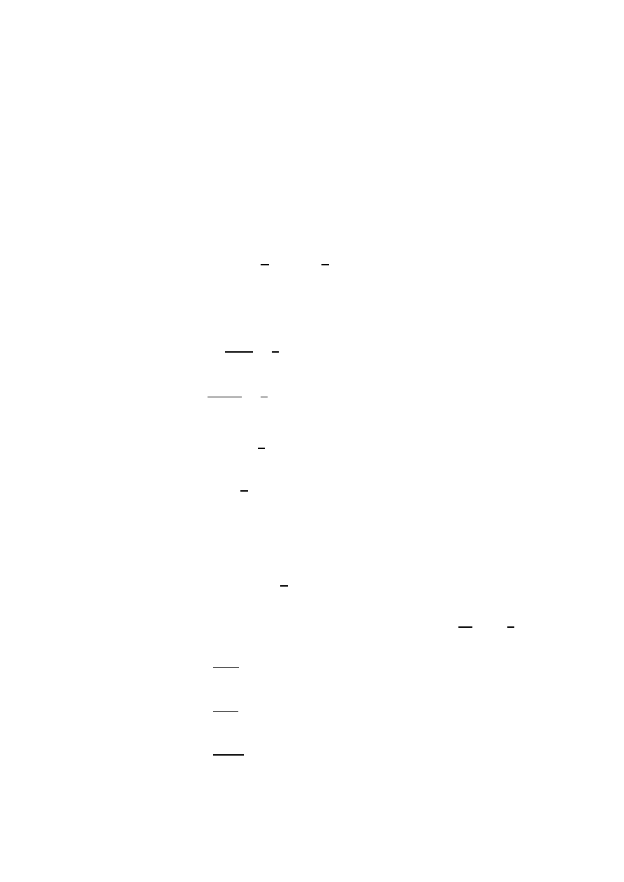
Miscellaneous Problems
1. Show that
n
X
d=1
(2d
− 1)
j
n
d
k
=
n
X
d=1
j
n
d
k
2
.
2. Show that
X
d
|n
τ (d)
3
=
X
d
|n
τ (d)
2
.
3. Show that
X
(a,b)=1
1
(ab)
2
=
5
2
.
4. Show that
Y p
2
+ 1
p
2
− 1
=
5
2
. (The product runs over all primes.)
5. Generalize the results of Problems 3 and 4 above.
6. Show that lim
n
→∞
X
d
|(n!+1)
1
d
= 1.
7. Show that lim
n
→∞
X
d
|F
n
1
d
= 1, where F
n
= 2
2
n
+ 1.
8. Prove that π(x) =
x
X
n=1
n
X
j=1
e
2πi((n
−1)!+1)j/n
.
9. Prove that (a, b) =
a
−1
X
m=0
a
−1
X
n=0
1
a
e
2πibmn/a
.
10. Show that the least absolute remainder of a (mod b) is a
−b
2a
b
+b
j
a
b
k
.
11. Prove that
∞
X
n=1
ϕ(n)
n!
is irrational.
12. Prove that
∞
X
n=1
σ(n)
n!
is irrational.
13. Prove that
∞
X
n=1
σ
2
(n)
n!
is irrational.
76
Miscellaneous Problems
14. Show that
x
X
n=1
n
σ(n)
≥ x + 1.
15. Show that
X
d
2
|n
µ(d) =
|µ(n)|.
16. Show that for g
6= 3, 1 + g + g
2
+ g
3
+ g
4
is not a square.
17. For n an integer and a
≥ 0 prove that
n
−1
X
k=0
a +
k
n
=
bnac.
18. Show that
1
φ(n)
=
1
n
X
d
|n
µ
2
(d)
φ(d)
.
19. Prove that
∞
X
n=1
µ(n)x
n
1 + x
n
= x
− 2x
2
.
20. Prove that
λ(n)x
n
1
− x
n
=
∞
X
n=1
x
n
2
.
21. Prove that F (n) =
Y
d
|n
f (d) if and only if f (n) =
Y
d
|n
F
n
d
µ(d)
.
22. Show that the sum of the odd divisors of n is
−
X
d
|n
(
−1)(
n
d
)d.
23. Prove that the product of the integers
≤ n and relatively prime to n is
n
ϕ(n)
Y n!
d
d
µ
n
d
.
24. Show that every integer has a multiple of the form 11 . . . 1100 . . . 00.
25. Prove that there are infinitely many square-free numbers of the form
n
2
+ 1.
26. Prove that
m
0
+
m
3
+
m
6
+
· · · 6≡ 0 (mod 3).
27. Show that the number of representations of n as the sum of one or more
consecutive positive integers is τ (n
1
) where n
1
is the largest odd divisor
of n.
28. Prove that ϕ(x) = n! is solvable for every n.
29. Prove that ϕ(x) = 2
· 7
n
is not solvable for any positive n.
30. Prove that 30 is the largest integer such that every integer less than it
and relatively prime to it is 1 or a prime.
31. Let a, b, x be integers and let x
0
= x, x
n+1
= ax
n
+ b (n > 0). Prove that
not all the x’s are primes.
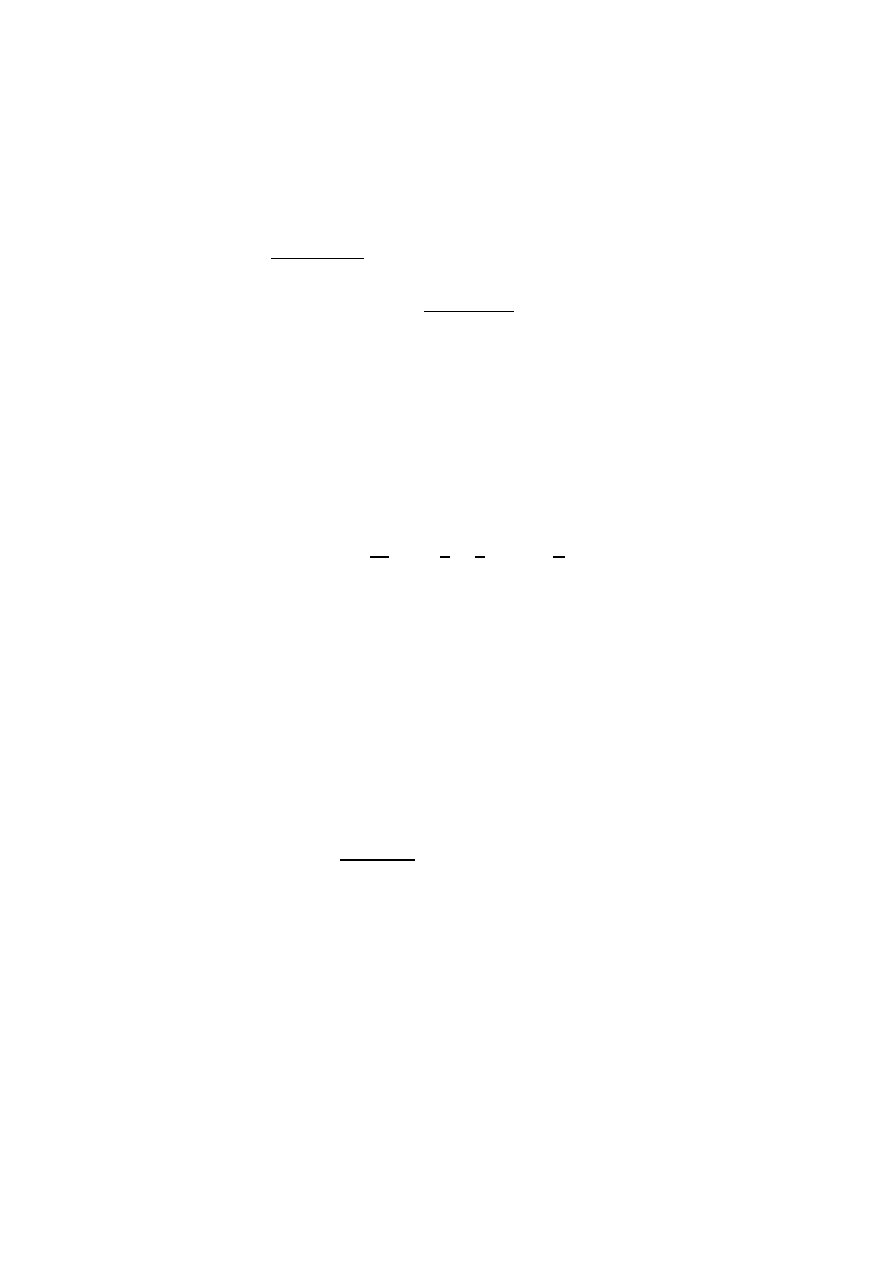
Miscellaneous Problems
77
32. Show that the only solutions of ϕ(n) = π(n) are n = 2, 3, 4, 8, 14, 20, 90.
33. Show that ϕ(n + 1) = p
n+1
− p
n
is valid only for 1
≤ n ≤ 5.
34. Show that
(2a)! (2b)!
a! b! (a + b)!
is an integer.
35. Show that if (a, b) = 1 is then
(a + b
− 1)!
a! b!
is an integer.
36. Show that an integral polynomial of at least the first degree cannot rep-
resent only primes.
37. Show that if f (x) is an integral polynomial of degree > 0, then f (x) for
x = 1, 2, . . . has an infinite number of distinct prime divisors.
38. Find the number of integers prime to m in the set
{1·2, 2·3, . . . , m·(m+1)}.
39. Prove that the Fermat numbers are relatively prime in pairs.
40. Let T
1
= 2, T
n+1
= T
2
n
− T
n
−1
. Prove that (T
i
, T
j
) = 1, i
6= j.
41. Prove that 2ζ(3) =
∞
X
n=1
1
n
2
1 +
1
2
+
1
3
+
· · · +
1
n
.
42. Prove that the density of numbers for which (n, ϕ(n)) = 1 is zero.
43. Show that for some n, 2
n
has 1000 consecutive 7’s in its digital represen-
tation.
44. Prove that infinitely many squares do not contain the digit 0.
45. Show that for some n, p
n
contains 1000 consecutive 7’s in its digital
representation.
46. Show that the density of the numbers n for which ϕ(x) = n is solvable is
zero.
47. Show that if ϕ(x) = n has exactly one solution then n > 10
100
.
48. Prove that e
p
(n) =
n
− s
p
(n)
p
− 1
.
49. Let a
1
, a
2
, . . . , a
p
−1
be ordered by not necessarily distinct nonzero residue
classes (mod p). Prove that there exist 1
≤ i ≤ j ≤ p − 1 such that
a
i
· a
i+1
· · · · · a
j
≡ 1 (mod p).
50. Show that the n
th
prime is the limit of the sequence
n
0
= n, n
k+1
= n
0
+ π(n
0
+ n
1
+
· · · + n
k
).
51. Show that the n
th
nonprime is the limit of the sequence
n, n + π(n), n + π(n + π(n)), . . . .
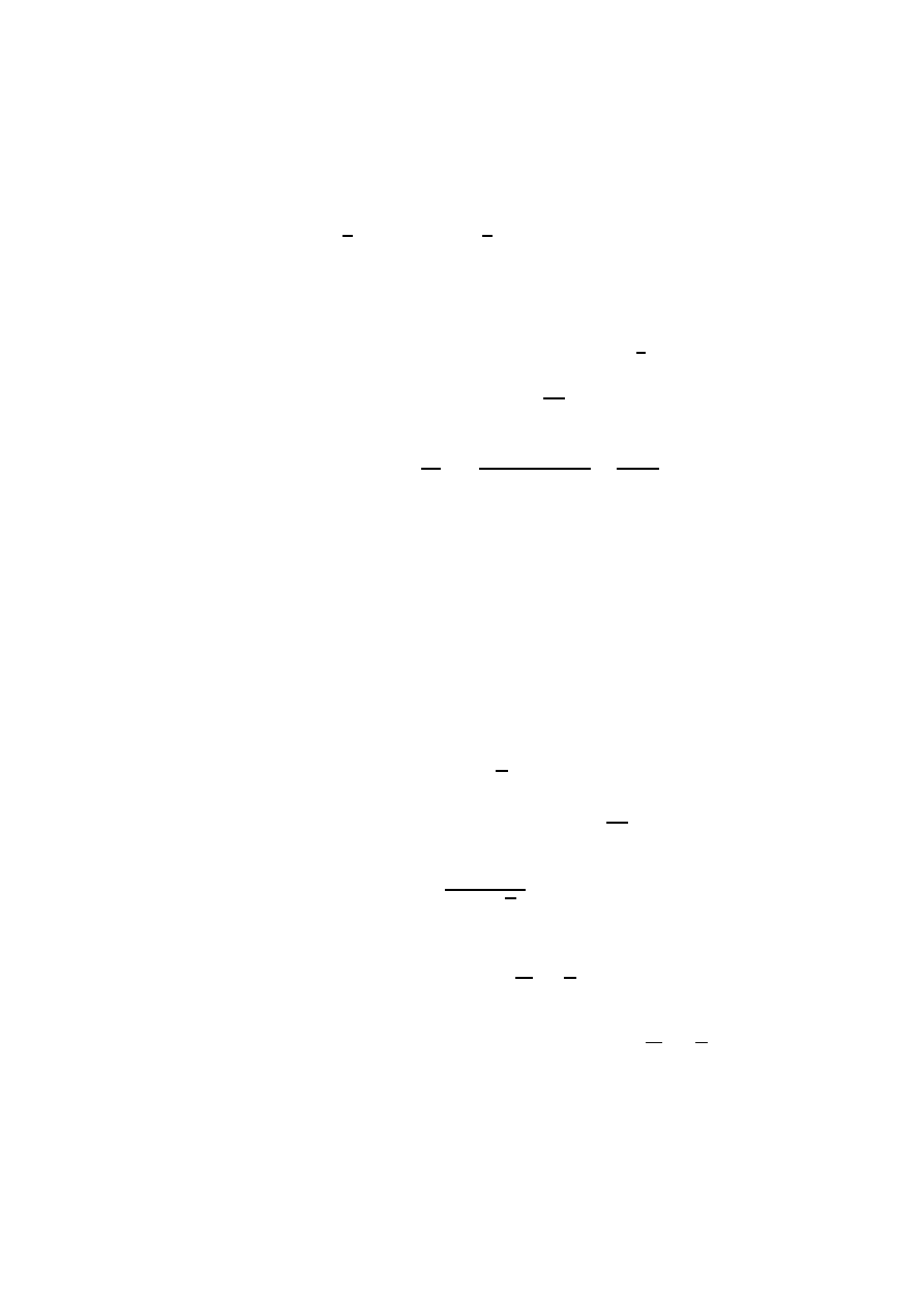
78
Miscellaneous Problems
52. Prove that every positive integer is either of the form n + π(n
− 1) or of
the form n + p
n
, but not both.
53. Show that (3 + 2
√
2)
2n
−1
+ (3
− 2
√
2)
2n
−1
− 2 is square for every n ≥ 1.
54. Prove that for every real ε > 0 there exists a real α such that the fractional
part of α
n
is greater than 1
− ε for every integer n > 0.
55. Show that if p and q are integers
≤ n, then it is possible to arrange n or
fewer unit resistances to give a combined resistance of
p
q
.
56. Show that (a, n) = 1 and x = a
− 12
X
k
≥1
k
ka
n
imply ax
≡ 1 (mod n).
57. If (a, b) = d prove that
a
−1
X
x=1
bx
a
=
(a
− 1)(b − 1)
2
+
d
− 1
2
.
58. Show that the sum of reciprocals of integers representable as sums of two
squares is divergent.
59. Show that the sum of reciprocals of integers whose digital representation
does not include 1000 consecutive 7’s is convergent.
60. Prove that every n > 1 can be expressed as the sum of two deficient
numbers.
61. Prove that every n > 10
5
can be expressed as the sum of two abundant
numbers.
62. Prove that every sufficiently large n can be expressed as the sum of two
k-abundant numbers.
63. Prove that the n
th
nonsquare is n+
{
√
n
}. ({x} denotes the integer closest
to x.)
64. Prove that the n
th
nontriangular number is n +
{
√
2n
}.
65. Prove that the n
th
non–k
th
power is
n +
k
q
n +
k
√
n
.
66. Show that the binary operation
◦ defined on nonnegative integers by
m
◦ n = m + n + 2b
√
m
cb
√
n
c
is associative.
67. Prove the same for the operation m
× n = m + n + 2{
√
m
}{
√
n
}.
68. Prove that for p > 5, (p
− 1)! + 1 contains a prime factor 6= p.
69. Show that the only solutions of (n
−1)! = n
k
−1 are (n, k) = (2, 1), (3, 1),
and (5, 2).
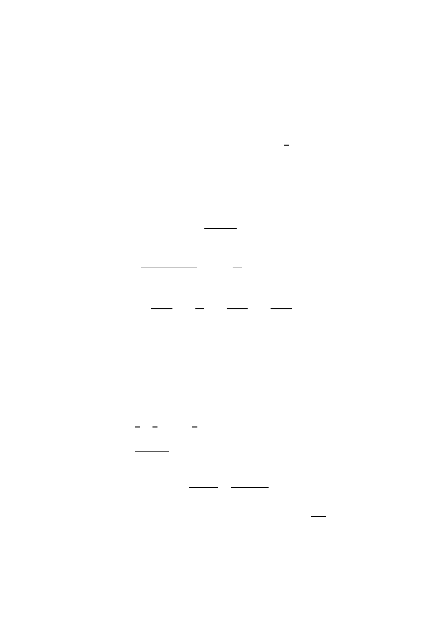
Miscellaneous Problems
79
70. Show that x
2
α
≡ 2
2
α
−1
(mod p) has a solution for every prime p if α
≥ 3.
71. Show that if f (x) is a polynomial with integer coefficients and f (a) is a
square for each a, then f (x) = (g(x))
2
, where g(x) is a polynomial with
integer coefficients.
72. Given integers a
1
< a
2
<
· · · < a
k
≤ n with k ≥ b
n
2
c, prove that for some
i
≤ j ≤ k, a
i
| a
j
.
73. Show that two of the a
i
’s of Problem 72 are relatively prime.
74. With the a’s of Problem 72, show that a
i
+ a
j
= a
k
is solvable.
75. Show that the number of solutions of x + 2y + 3z = n in non negative
integers is
(n + 3)
2
12
.
76. Show that the number of solutions of x + 2y + 4z = n in non negative
integers is
(n + 2)(n + 5)
16
+ (
−1)
n
n
16
.
77. Show that n and n + 2 are simultaneously prime if and only if
X
m
≥1
n + 2
m
+
n
m
−
n + 1
m
−
n
− 1
m
= 4.
78. Show that n and n + 2 are simultaneously prime if and only if
4(n
− 1)! + 1 + n ≡ 0 (mod n(n + 2)), (n > 1).
79. Show that for every n, 6
· 10
n+2
, and 1125
· 10
2n+1
± 8 are Pythagorean
triples.
80. Show that the number of ordered pairs of integers whose l.c.m. is n is
τ (n
2
).
81. Show that
1
2
+
1
3
+
· · · +
1
n
is never an integer.
82. Show that
x
2
+ 2y
2
2x
2
+ y
2
is a square if and only if x = y.
83. Prove that
∞
X
n=1
ϕ(n)x
n
1 + x
n
=
x(1 + x
2
)
(1
− x
2
)
2
.
84. Show that the number of regular n-gons of unit edge is
ϕ(n)
2
.
85. Prove that the n
th
order determinant with a
ij
= (i, j) has value
n
Y
i=1
ϕ(i).
80
Miscellaneous Problems
86. Prove that
n
X
i=1
√
i
=
√
n
3n + 1 − {
√
n
}
2
3
.
87. Prove that if p = 4n + 3 and q = 8n + 7 are both prime then q
| 2
p
− 1.
88. Show how to split the positive integers into two classes so that neither
class contains all the positive terms of any arithmetic progression with
common difference exceeding 1.
89. Show that the reciprocal of every integer n > 1 can be expressed as the
sum of a finite number of consecutive terms of the form
1
j(j+1)
.
90. In how many ways can this be done? (Answer:
1
2
(τ (n
2
)
− 1).)
91. Show that every rational can be expressed as a sum of a finite number of
distinct reciprocals of integers.
92. Show that the density of integers for which (n,
b
√
n
c) = 1 is
6
π
2
.
93. Show that the expected value of (n,
b
√
n
c) is
π
2
6
.
94. Prove that x
2
≡ a (mod p) for every prime p implies that a is a square.
95. Prove that f (a, b) = f (a)f (b) for (a, b) = 1 and f (a + 1)
≥ f(a) for every
a imply that f (a) = a
k
.
96. Find all primes in the sequence 101, 10101, 1010101, . . . .
97. Find all primes in the sequence 1001, 1001001, 1001001001, . . . .
98. Show that if f (x) > 0 for all x and f (x)
→ 0 as x → ∞ then there exists
at most a finite number of solutions in integers of f (m) + f (n) + f (p) = 1.
99. Prove that the least nonresidue of every prime p > 23 is less than
√
p.
100. Prove the existence of infinite sequences of 1’s, 2’s, and 3’s, no finite part
of which is immediately repeated.
101. Let d
∗
(n) denote the number of square divisors of n. Prove that
lim
n
→∞
1
n
n
X
m=1
d
∗
(m) =
π
2
6
.
102. Find all r such that n! cannot end in r zeros.
103. Let a
1
, a
2
, . . . , a
n
be integers with a
1
= 1 and a
i
< a
i+1
≤ 2a
i
. Prove
that there exists a sequence
{ε
i
} of ±1’s such that
n
X
i=1
ε
i
a
i
= 0 or 1.
104. Show that for p a prime, p
≡ 1 (mod 4)
b
√
p
c +
jp
2p
k
+
· · · +
$r
p
− 1
4
· p
%
=
p
2
− 1
12
.
Miscellaneous Problems
81
105. Prove that π
2
is irrational.
106. Prove that cos
p
q
is irrational.
107. If
n
i
n
1
n
2
. . . n
i
−1
→ ∞ prove that
X 1
n
i
is irrational.
108. Prove that ae
2
+ be + c
6= 0 if a, b, c are integers.
109. Prove that
τ (n) =
√
n
−
√
n
− 1
+ 2
b
√
n
−1
c
X
d=1
j
n
d
k
−
n
− 1
d
.
110. Let n = a
0
+ a
1
p + a
2
p
2
+
· · · + a
k
p
k
where p is a prime and 0
≤ a
i
< p.
Show that the number of binomial coefficients of order n that are relatively
prime to p is
Q
(a
i
+ 1).
111. Show that if r
1
, r
2
, . . . , r
p
−1
form a complete residue system (mod p) then
1r
1
, 2r
2
, . . . , (p
− 1)r
p
−1
do not.
112. Show that 3 is a primitive root of every Fermat prime.
113. Show that the number of ways in which n can be represented as the
product of two relatively prime factors is 2
ω(n)
−1
.
114. Prove that every even perfect number is of the form 2
p
−1
(2
p
− 1).
115. Show that if f (x) is a polynomial with integral coefficients and there are
ψ(m) integers relatively prime to m in the set
{f(1), f(2), . . ., f(m)} then
ψ is a weakly multiplicative function.
116. If p = 4n + 1 is a prime, show that (2n)!
2
+ 1
≡ 0 (mod p).
117. Show that 128 is the largest integer not representable as the sum of dis-
tinct squares.
118. Show that x
3
+ y
4
= z
5
has infinitely many solutions.
119. Show that x
n
+ y
n
= x
n+1
has infinitely many solutions.
120. Show that for every k > 0 there exists a lattice point (x
1
, y
1
) such that for
every lattice point (x, y) whose distance from (x
1
, y
1
) does not exceed k,
the g.c.d. (x, y) > 1.
121. Prove that no four distinct squares are in arithmetic progression.
122. Prove that for n composite, π(n) <
n
log n
.
123. Prove that 2
n
| {(n +
√
5)
n
}.
124. Prove that an odd p is prime if and only if p + k
2
is not a square for
k = 1, 2, . . . ,
p
−3
2
.

Unsolved Problems and Conjectures
1. Does ϕ(n) = ϕ(n + 1) have infinitely many solutions?
2. Does σ(n) = σ(n + 1) have infinitely many solutions?
3. Does ϕ(n) = ϕ(n+1) =
· · · = ϕ(n+k) have solutions for every k? (Erd˝os)
4. Conjecture: There is no n for which ϕ(x) = n has a unique solution.
(Carmichael)
5. Conjecture: For every positive integer k > 1 there exist infinitely many
n for which ϕ(x) = n has exactly k solutions.
6. Do there exist solutions of σ(n) = 2n + 1 ?
7. Is ϕ(x) = ϕ(y) = 2n solvable for every n ? (Moser)
8. Are there infinitely many solution of τ (n) = τ (n + 1)?
9. Are there infinitely many numbers not of the form φ(n) + n? (Erd˝
os)
10. Are there infinitely many numbers not of the form σ(n) + n? (Erd˝
os)
11. Do there exist solutions of σ(x) = mσ(y) for every integer m? (Sierpinski)
12. Are 1, 2, 4, 8, and 128 the only powers of 2, all of whose digits are powers
of 2? (Starke)
13. Does there exist for every n, n distinct integers all of whose sums in pairs
are squares? (This is true for n
≤ 5.)
14. Does there exist a sequence of
{ε
i
} of ±1’s such that
P
n
i=1
ε
i
·k
is bounded
for every k? (Erd˝
os)
15. If f (n) is an arithmetic function of period k and not identically 0, is it
true that
P
f (n)
n
6= 0? (Erd˝os)
16. Conjecture: For n sufficiently large, n can be partitioned n = a+b+c+d =
d + e + f with abc = def . (Motzkin)
17. Is
∞
X
n=1
σ
k
(n)
n!
irrational for every k? (Erd˝
os and Kac)
18. Is
1
x
+
1
y
+
1
z
=
4
n
solvable for every n? (Erd˝
os)
19. Has n! + 1 = x
2
any solutions with n > 7? (Brochard)
84
Unsolved Problems and Conjectures
20. Is
(2n)!
(n + 2)!
2
an integer for infinitely many n? (Erd˝
os)
21. Is
(2n)!
n! (n + k)!
an integer for every k and infinitely many n? (Erd˝
os)
22. Does there exist an A such that
bA
n
c is prime for every n? (Mills)
23. Does
be
n
c represent infinitely many primes?
24. Does
be
n
c represent infinitely many composite numbers? (Erd˝os)
25. The number 105 has the property that 105
− 2
n
is prime whenever it is
positive. Is 105 the largest number with this property?
26. Is 968 the largest number n such that for all k with (n, k) = 1 and n > k
2
,
n
− k
2
is prime? (Erd˝
os)
27. Does there exist a prime p > 41 such that x
2
− x + p is prime for 1 ≤ x ≤
p
− 1?
28. Let α(n) denote the number of 1’s in the binary representation of n.
Does there exist a k such that for infinitely many primes p, α(p) < k?
(Bellman)
29. If f (x) is a polynomial with integer coefficients, f
0
(a) = a, and f
n+1
(a) =
f (f
n
(a)), can a sequence f
n
(a), n = 1, 2, . . . consist entirely of primes?
30. For p sufficiently large and ab
6= 0, n > 2, does the polynomial x
n
+ ax + b
assume more than
p
2
values (mod p)? (Chowla)
31. Find pairs of integers m, n such that m, n have the same prime factors
and m + 1, n + 1 have the same prime factors; e.g., m = 2
k
− 2 and
n = 2
k
(2
k
− 2). Are these the only cases? (Strauss)
32. What is the largest integer not representable as the sum of distinct cubes?
33. Let 1 < u
1
< u
2
<
· · · be the sequence of integers of the form x
2
+ y
2
.
Conjecture:
lim
n
→∞
u
n+1
− u
n
u
1/4
n
= 0.
(Chowla and Davenport)
34. Conjecture:
X
n
≤x
(
−1)
n
−1
p
n
∼
p
x
2
. (Pillai)
35. Can every prime p
≡ 3 (mod 8), p > 163, be written as the sum of three
distinct squares? (Chowla)
36. Is ζ(3) irrational?
1
Is ζ(2s + 1) irrational?
1
Publisher’s note: Ap´
ery proved in 1978 that ζ(3) is irrational; see “A proof that Euler
missed . . . Ap´
ery’s proof of the irrationality of ζ(3): An informal report” by A. J. van der
Poorten, Mathematical Intelligencer 1, no. 4, 1978/79, pp. 195–203..
Unsolved Problems and Conjectures
85
37. Conjecture: The only solution of 1
n
+2
n
+
· · ·+m
n
= (m+1)
n
is 1+2 = 3.
(Bowen)
38. Conjecture: The only solutions of a
n
+(a+1)
n
+
· · ·+(a+b)
n
= (a+b+1)
n
are 1 + 2 = 3, 3
2
+ 4
2
= 5
2
, and 3
3
+ 4
3
+ 5
3
= 6
3
. (Erd˝
os)
39. Does the equation 1
2
+ 2
2
+
· · ·+m
2
= (m + 1)
2
+
· · ·+n
2
have solutions?
(Kelly)
40. The product of n > 1 consecutive integers is not a k
th
power.
41. Conjecture: If α > 0 is not an integer then the density of solutions of
(n, n
α
) = 1 is 6/π
2
. (Lambek and Moser)
42. Conjecture: The only solutions of
1
x
1
+
1
x
2
+
· · · +
1
x
n
+
1
x
1
x
2
. . . x
n
= 1
are
1
2
+
1
2
=
1
2
+
1
3
+
1
6
=
1
2
+
1
3
+
1
7
+
1
42
= 1.
(Erd˝
os)
43. Is it true that for all pairs of primes p, q all sufficiently large numbers can
be written as the sum of distinct numbers of the form p
α
q
β
? (Erd˝
os)
44. Let a
1
, a
2
, . . . be integers not exceeding n such that the l.c.m. of any two
is > n . What in the maximum of
P
1
a
i
? Conjecture: 31/30. (Erd˝
os)
45. Let 0 < a
1
< a
2
<
· · · < a
k
≤ n be such that the sums of distinct a
i
’s are
distinct. Conjecture: k
− log
2
n is bounded. (Erd˝
os)
46. Give a relatively simple proof of Van der Waerden’s theorem for the case
of two classes.
47. Give a relatively simple proof of Roth’s theorem: Any sequence that does
not contain an arithmetic progression has zero density.
48. Give an elementary proof of Dirichlet’s theorem on quadratic residues:
X n
p
> 0
for p
≡ 3 (mod 4).
49. Let a
1
< a
2
< . . . be a sequence of positive integers and let f (n) denote
the number of solutions of a
i
+ a
j
= n. Conjecture: If f (n) > 0 for every
n then f (n) is unbounded. (Erd˝
os and Turan)
50. If the f (n) of Problem 49 is > 0 for every n then every sufficiently large
n can be written as the sum of three distinct a’s. (Kelly)
51. Construct a sequence of a’s for which the f (n) of Problem 49 is > 0 and
for which f (n) < log n for every n. (Erd˝
os has shown that such sequences
exist.)
86
Unsolved Problems and Conjectures
52. Does there exist a sequence A with counting function A(n) < cn/ log n
such that every integer can be represented in the form a + 2
i
, a
∈ A?
53. Improve the bound [n! e] in Schur’s theorem in combinatorial number
theory.
54. Conjecture. If a
1
< a
2
<
· · · is a sequence of integers with a
n
/a
n+1
→ 1
and if for every d, every residue (mod d) is representable as the sum of
distinct a’s, then at most a finite number of integers are not representable
as the sum of distinct a’s. (Erd˝
os)
55. Is the sum of the reciprocals of those integers that are representable as
the sum of k k
th
powers divergent? (Klamkin and Newman)
56. Conjecture: For every ε > 0 there exists an N = N (ε) such that for
n > N the n-dimensional game of tic-tac-toe played on a 3
× 3 × · · · × 3
board must terminate before ε3
n
moves have been played. (Moser)
57. Same as Problem 56 with 3 replaced by k.
58. Every integer belongs to one of the arithmetic progressions
{2n}, {3n},
{4n+1}, {6n+5}, {12n+7}, n = 1, 2, . . . . This is the simplest example of
a finite set of arithmetic progressions, each with different common differ-
ence, all of whose common differences are greater than one, that contain
all integers. Does there exist for every c > 0 such a set of progressions,
each common difference being > c? (Erd˝
os)
59. Give an explicit representation of n as the sum of four squares.
60. Do there exist for every n, n primes that are consecutive terms of an
arithmetic progression?
61. Let
1
1 + x + 2x
2
=
∞
X
n=1
a
n
x
n
. Conjecture:
|a
n
| > c log log n.
62. Are there infinitely primes of the form 11
· · · 11 ?
63. Are there infinitely many Euclid primes 2
· 3 · · · · · p
n
+ 1?
64. Conjecture: The least nonresidue of a prime p is < c log p.
65. Conjecture: The least primitive root of a prime p is < p
ε
, p > p
0
(ε).
66. Conjecture: The number of perfect numbers
≤ n is < c log n.
67. Find good bounds for the density of the abundant numbers.
68. Prove that the ratio of residues to nonresidues in the range (1, [
√
p]) ap-
proaches 1 as p
→ ∞.
69. Give an elementary proof of
Y
p
≤n
p < 3
n
.
70. Conjecture: lim
n
→∞
(a
n+1
− a
n
) =
∞ implies
X
n=1
a
n
2
a
n
irrational. (Erd˝
os)
Unsolved Problems and Conjectures
87
71. Find all solutions of x
4
+ y
4
= z
4
+ t
4
.
72. Find all solutions of x
4
+ y
4
+ z
4
= t
4
.
73. Find all solutions of x
x
y
y
= z
z
.
74. Let `(n) be the least r for which there exists a chain of integers
a
0
= 1 < a
1
< a
2
<
· · · < a
r
= n,
where for each i > 0, a
i
= a
j
+ a
k
for some j, k < i (j = k permitted).
Conjecture: `(2
q
− 1) ≤ q + `(q) − 1. (Scholz)
75. Conjecture: `(n) < `(2n) for all n > 0. (Utz)
76. Let S(n) denote the number of solutions of `(x) = n. Is it true that
S(n) < S(n + 1) for all n > 0? (Utz)
77. Polya’s conjecture:
x
X
n=1
λ(n)
≤ 0, x > 1. (Checked for x < 800,000.)
78. Turan’s conjecture:
x
X
n=1
λ(n)
n
> 0. (Checked for x < 50,000.)
79. Pillai’s conjecture:
|x
m
− y
n
| < N, m, n > 1 has for every N only a finite
number of solutions.
80. 2
e
is irrational.
81. Find a reasonable estimate for the number of solutions in positive integers
of
1
x
1
+
1
x
2
+
1
x
3
+
· · · +
1
x
n
= 1.
Document Outline
- An Introduction to the Theory of Numbers
- Terms and Conditions
- Contents
- Preface
- 1 Compositions and Partitions
- 2 Arithmetic Functions
- 3 Distribution of Primes
- 4 Irrational Numbers
- 5 Congruences
- 6 Diophantine Equations
- 7 Combinatorial Number Theory
- 8 Geometry of Numbers
- Classical Unsolved Problems
- Miscellaneous Problems
- Unsolved Problems and Conjectures
Wyszukiwarka
Podobne podstrony:
Sapir (1921) Language an Introduction to the Study of Speech
0198752091 Oxford University Press USA The Character of Mind An Introduction to the Philosophy of Mi
An Introduction to the Phenomenology of Signs
AN INTRODUCTION TO THE HISTORY OF KHAZARIA(1)
Bryce Gilmore An Introduction To The Methods Of Wd Gann
An introduction to the Analytical Writing Section of the GRE
SCHAFER, Christian The Philosophy of Dionysius the Areopagite an introduction to the structure and
An Introduction to the Kabalah
Zinda; Introduction to the philosophy of science
Geiss An Introduction to Probability Theory
Cognitive Psychology from Hergenhahn Introduction to the History of Psychology, 2000
Introduction To The Metaphysic Of Morals
An Introduction to the Kabalah
Dedekind, Richard Essays on the Theory of Numbers [pdf]
Truth and Knowledge Introduction to The Philosophy of Freedom by Rudolf Steiner
więcej podobnych podstron