A Study of Detecting Computer Viruses in Real Infected Files in the n gram Representation with Machine Learning Methods

A Study of Detecting Computer Viruses in

Real-Infected Files in the n-gram

Representation with Machine Learning Methods

Note, this is an extended version. The LNCS published version is

available via springerlink

Thomas Stibor

Fakult¨

at f¨

ur Informatik

Technische Universit¨

at M¨

unchen

thomas.stibor@in.tum.de

Abstract.

Machine learning methods were successfully applied in re-

cent years for detecting new and unseen computer viruses. The viruses
were, however, detected in small virus loader files and not in real infected
executable files. We created data sets of benign files, virus loader files and
real infected executable files and represented the data as collections of
n-grams. Histograms of the relative frequency of the n-gram collections
indicate that detecting viruses in real infected executable files with ma-
chine learning methods is nearly impossible in the n-gram representation.
This statement is underpinned by exploring the n-gram representation
from an information theoretic perspective and empirically by performing
classification experiments with machine learning methods.

Introduction

Detecting new and unseen viruses with machine learning methods is a challenging
problem in the field of computer security. Signature based detection provides
adequate protection against known viruses, when proper virus signatures are
available. From a machine learning point of view, signature based detection is
based on a prediction model where no generalization exists. In other words,
no detection beyond the known viruses can be performed. To obtain a form of
generalization, current anti-virus systems use heuristics generated by hand.

In recent years, however, machine learning methods are investigated for de-

tecting unknown viruses [1–5]. Reported results show high and acceptable de-
tection rates. The experiments, however, were performed on skewed data sets,
that is, not real infected executable files are considered, but small executable
virus loader files. In this paper, we investigate and compare machine learning
methods on real infected executable files and virus loader files. Results reveal
that real infected executable files when represented as n-grams can barely be
detected with machine learning methods.

Data Sets

In this paper, we focus on computer virus detection in DOS executable files.
These files are executable on DOS and some Windows platforms only and can
be identified by the leading two byte signature “MZ” and the file name suffix
“.EXE”. It is important to note that although DOS platforms are obsolete, the
princinple of virus infection and detection on DOS platforms can be generalized
to other OS platforms and executable files.

In total three different data sets are created. The benign data set consists

of virus-free executable DOS files which are collected from public FTP servers.
The collected files consist of DOS games, compilers, editors, etc. and are prepro-
cessed such that no duplicate files exist. Additionally, files that are compressed
with executable packers

such as lzexe, pklite, diet, etc. are uncompressed. The

preprocessing steps are performed to obtain a clean data set which is supposed
to induce high detection rates of the considered machine learning methods. In
total, we collected 3514 of such “clean” DOS executable files.

DOS executable virus loader files are collected from the VXHeaven website.

The same processing steps are applied, that is, all duplicate files are removed
and compressed files are uncompressed. It turned out however, that some files
from VXHeaven are real infected executable files and not virus loader files. These
files can be identified by inspecting their content with a disassembler/hexeditor
and by their large file sizes. Consequently, we removed all files greater than 10
KBytes and collected in total 1555 virus loader files.

For the sake of clarity, the benign data set is denoted as B

files

, the virus

loader data set as L

files

The data set of real infected executable files denoted as I

files

is created by

performing the following steps:

files

:= {}

2: for each file.v in

files

setup new DOS environment in DOS emulator

randomly determine file.r from

files

boot DOS and execute file.v and file.r

if (file.r gets infected)

files

:= I

files

∪ {file.r}

Fig. 1.

Steps performed to create real infected executable DOS files.

These steps were executed on a GNU/Linux machine by means of a Perl script
and a DOS emulator. A DOS emulator is chosen since it is too time consuming
to setup a clean DOS environment on a DOS machine whenever a new file gets

Executable compression is frequently used to confuse and hide from virus scanners.

Available at http://vx.netlux.org/

infected. The statement “file.r gets infected” at line 6 in Figure 1 denotes
the data labeling process. Since only viruses were considered for which signatures
are available, no elements in the created data sets are mislabeled. In total 1215
real infected files were collected.

Transforming Executable Files to n-grams and
Frequency Vectors

Raw executable files cannot serve properly as input data for machine learning
methods. Consequently, a suitable representation is required. A common and
frequently used representation is the hexdump. A hexdump is a hexadecimal
representation of an executable file (or of data in general) and is related to ma-
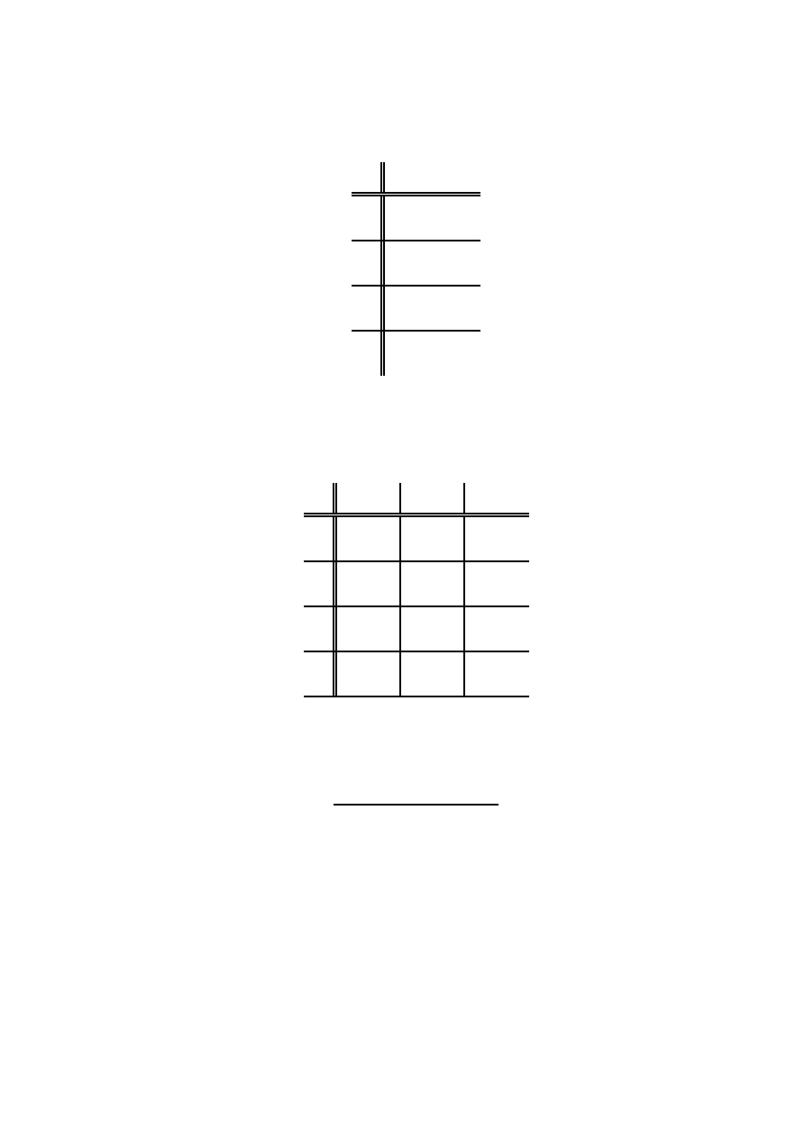
chine instructions, termed opcodes. Figure 2 illustrates the connection between
machine instructions, opcodes, and a hexdump. It is important to note, that the
hexdump representation used and reported in the literature, is computed over
a complete executable file which consists of a header, relocation tables and the
executable code. The machine instructions are located in the code segment only
and this implies that a hexdump obtained over a complete executable file may
not be interpreted completely as machine instructions.

machine instruction

opcode

mov bx, ds

8CDB

push ebx

add ebx, 2E

83C32E

nop

8CDB5383C32E90

hexdump

Fig. 2.

Relation between machine instructions, opcodes and the resulting hexdump.

In the second preprocessing step, the hexdump is “cut” into substrings of

length n ∈ N, denoted as n-grams. According to the literature an n-gram can be
any set of characters in a string [6]. In terms of detecting viruses in executable
files, n-grams are adjacent substrings created by shifting a window of length
s ∈ N over the hexdump. The resulting number of created n-grams depends on
the value of n and the window shift length s.

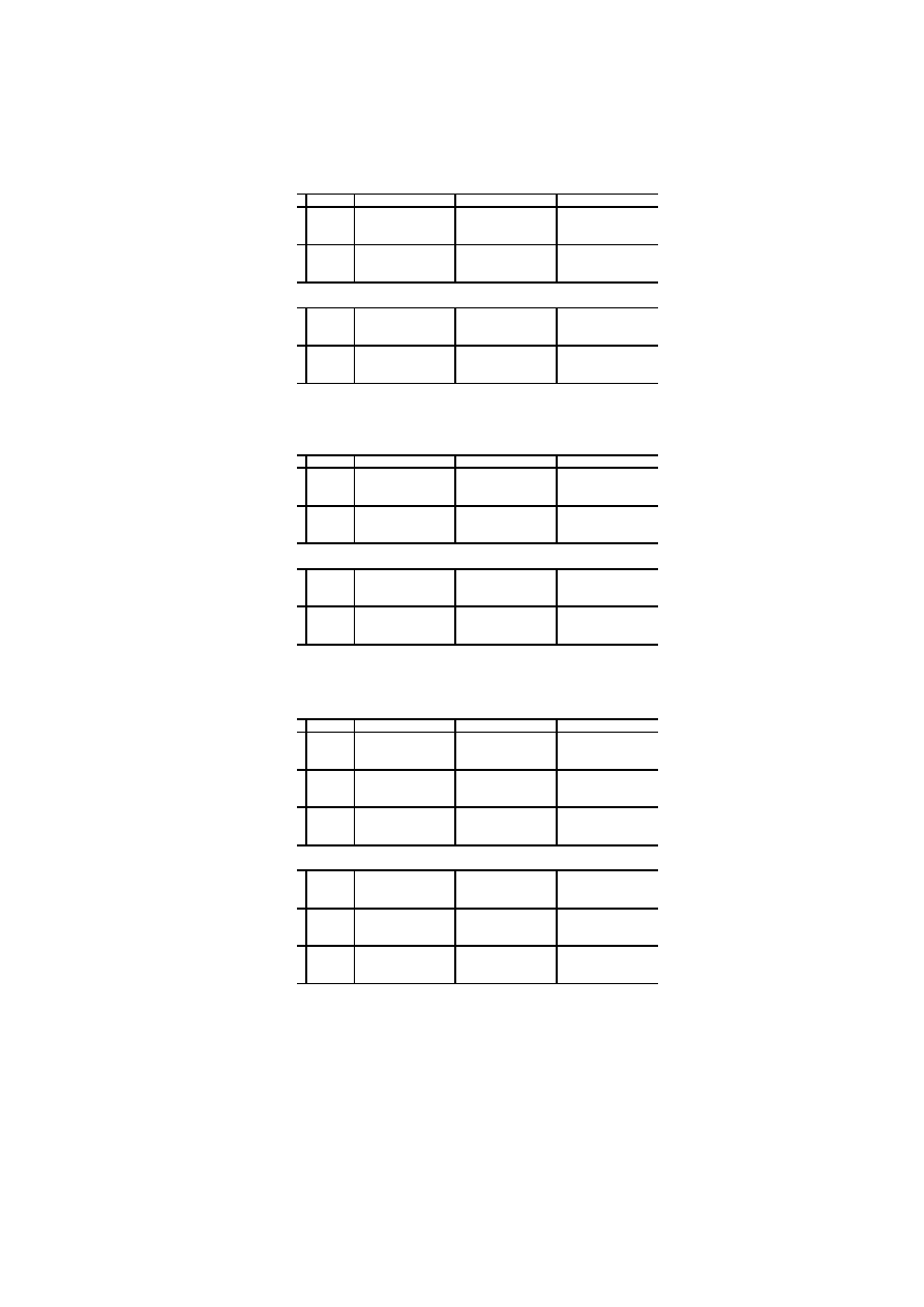
We created for each file an ordered collection

of n-grams by cutting the

hexdump from left to right (see Fig. 3). Note that the collection can contain the
same n-grams multiple times. The total number of n-grams in the collection when
given n and s is ⌊(l − n)/s + 1⌋, where l denotes the hexdump length. In a final
step, the collection is transformed into a vector of dimension

d = 16

, where

For

the

sake

verifiability,

the

three

data

sets

are

available

http://www.sec.in.tum.de/

∼stibor/ieaaie2010/

If not otherwise stated we denote an ordered collection as collection.

An unary hexadecimal number can take 16 values.

8 C D B 5 3 8 3 C 3 2 E 9 0
8 C D B

C D B 5

D B 5 3

3 2 E 9

2 E 9 0

8 C D B 5 3 8 3 C 3 2 E 9 0
8 C D B

D B 5 3

5 3 8 3

C 3 2 E

2 E 9 0

n = 4, s = 1

{8CDB,CDB5,DB53,. . .,32E9,2E90}

n = 4, s = 2

{8CDB,DB53,5383,. . .,C32E,2E90}

Fig. 3.

Resulting n-grams and collections for n = 4 and different window shift lengths

(s = 1 and s = 2).

each component corresponds to the absolute frequency of the n-gram occurring
in the collection (cf. Example 1). In the problem domain of text classification
such vectors are named term frequency vectors [7]. We therefore denote such
vectors as n-gram frequency vectors.

Example 1.

Given the n-gram collection

{B, 3, A, F, B, 7, B, B, 9, 7, 0}, where n = 1 and s = 1 and hence d = 16. The
corresponding vector results in
(1, 0, 0, 1, 0, 0, 0, 2, 0, 1, 1, 4, 0, 0, 0, 1), because n-gram “0” occurs one time in the
collection, n-gram “1” occurs zero times and so on.

Creating and Selecting of Informative n-grams

For large values of n, the created n-gram frequency vectors are limited process-
able due to their high-dimensional nature. In this section we therefore address
the problem of creating and selecting the most “informative” n-grams. More
precisely, the following two problems are addressed:

–

How to determine the parameters n and s such that the most “informative”
n-grams can be created?

–

How to select the most “informative” n-grams once they are created?

Both problems can be worked out by using arguments from information theory.

Let X be a random variable that represents the outcome of an n-gram and

X the set of all n-grams of length n. The entropy is defined as

H(X) =

x∈X

P (X = x) log

P (X = x)

(1)

Informally speaking, high entropy implies that X is from a roughly uniform
distribution and n-grams sampled from it are distributed all over the place.
Consequently, predicting sampled n-grams is “hard”. In contrast, low entropy
implies that X is from a varied distribution and n-grams sampled from it would
be more predictable.

4.1

Information Loss in Frequency Vectors

Given a hexdump of a file, the resulting n-gram collection C and the created
n-gram frequency vector c. We are interested in minimizing the amount of in-
formation loss for reconstructing the n-gram collection C when given c. For the
sake of simplicity we consider the case n = s and denote the cardinality of C as
t. Assume there are r unique n-grams in C, where each n-gram appears n

times

such that

r
i=1

= t. The collection C can have

! n

! · · · n

, n

, . . . , n

(2)

many rearrangements of n-grams. Applying the theorem from information theory
on the size of a type class [8], (pp. 350, Theorem 11.1.3) it follows:

(t + 1)

|Σ|

tH(P )

≤

, n

, . . . , n

≤ 2

tH(P )

(3)

where P denotes the empirical probability distribution of the n-grams, H(P )
the entropy of distribution P and Σ the used alphabet. Using n = s it follows
from (3) that 2

⌊l/n⌋H(P )

is an upper bound of the information loss. To keep the

upper bound as small as possible, the value of n has to be close to the value
of l and the empirical probability distribution P has to be a varied distribution
rather than a uniform distribution.

4.2

Entropy of n-gram Collections

To support the statement in Section 4.1 empirically, the entropy values of the
created n-gram collections are calculated. The values are set in relation to the
maximum possible entropy (uniform distribution) denoted as Hmax. An n-gram
collection where the corresponding value of H(X)/Hmax is close to zero, con-
tains more predictive n-grams than the one where H(X)/Hmax is close to one.
The results for different parameter combinations of n and s are listed in Ta-
ble 1. One can see that larger n-grams lengths are more predictable than short

ones. Additionally, one can observe that window shift length s has to be a mul-
tiple of two, because opcodes most frequently occur as two and four byte values.
Moreover, one can observe that the result of H(X)/Hmax for n-gram collections
created from the benign set B

files

and virus infected set I

files

have approximately

the same values. In other words, discriminating between those two classes is
limited realizable. This observation is also identifiable in Section 6 where the
classification results are presented and by inspecting Figure 4 which shows his-
tograms of the relative frequencies of the n-grams. From a practical point of
view, however, large values of n induce a computational complexity which is not
manageable. To be more precise, the crucial factor that influences the computa-
tional complexity is not just the total number of created n-grams (see Table 2),
but also the number of unique n-grams, that is, the lower bound of the dimen-
sion of the frequency vector. For our data sets we obtained the results listed in
Table 3. One can observe that all possible n-grams occurred in the collections.
As a consequence, we focus in the paper on n-gram lengths 2 and 3. We tried to
run the classification experiments for n = 4, 5, 6, 7, 8 in combination with a di-
mensionality reduction described in the subsequent section, however, due to the
resulting space complexity and lack of memory space

no results were obtained.

4.3

Feature Selection

The purpose of feature selection is to reduce the dimensionality of the data such
that the machine learning methods can be applied more efficiently in terms of
time and space complexity. Furthermore, feature selection often increases clas-
sification accuracy by eliminating noisy features. We apply on our data sets the
mutual information method [7]. This method is used in previous work and ap-
pears to be practical [5]. A comparison study of other feature selection methods
in terms of classifying malicious executables is provided in [9].

Mutual Information Selection:

Let U be a random variable that takes values

= 1 (the collection contains n-gram ng) and e

= 0 (the collection does not

contain ng). Let C be a random variable that takes values e

= 1 (the collection

belongs to class c) and e

= 0 (the collection does not belong to class c).

The mutual information measures how much information the presence/absence

of an n-gram contributes to making the correct classification decision on c. More
formally

(4)

∈{0,1}

P (U = e

, C = e

)

· log

P (U = e

, C = e

)

P (U = e

)P (C = e

)

A Quad-Core AMD 2.6 Ghz with 16 GB RAM was used.

0.923 0.896 0.862
0.924 0.895 0.861
0.738 0.679 0.628

0.889 0.857 0.818
0.888 0.857 0.816
0.708 0.649 0.593

0.896 0.862
0.895 0.860
0.679 0.626

0.816
0.813
0.590

Table 1.

Results of the expression H(X)/Hmax for different parameter combinations

of n and s. Smaller values indicate that more predictive n-grams can be created. The
upper value in each row denotes the result of n-grams created from benign set B

files

the middle value from virus infected set I

files

, the lower value from virus loader set

files

378 238 050 378 234 536 378 231 022
128 293 929 128 292 714 128 291 499

8 281 043

8 279 488

8 277 933

189 120 782 189 117 268 189 117 268

64 147 572 64 146 357 64 146 357

4 141 299

4 139 744

126 079 338 126 078 183

42 764 639 42 764 238

2 760 368

2 759 815

94 560 011
32 073 535

2 070 340

Table 2.

Number of created n-grams for different n-gram and window lengths s. The

upper number in each row denotes the number of n-grams created from benign set
B

files

, the middle number from virus infected set I

files

, the lower number from virus

loader set L

files

256 4096 65536 1048576

files

256 4096 65536 1048576

files

256 4096 65536 1048576

Table 3.

The number of unique n-grams of the three data sets B

files

, L

files

, I

files

. The

number determines the dimension of the corresponding frequency vectors.

Classification Methods

In this section we briefly introduce the classification methods which are used in
the experiments. These methods are frequently applied in the field of machine
learning.

5.1

Cosine Similarity Classification

Given two vectors x, y ∈ R

, the cosine similarity is given as follows

cos φ =

hx, yi

kxk kyk

(5)

+ . . . + x

+ . . . + y

(6)

The dot product of x and y denotes as hx, yi has a straightforward geometrical
interpretation, namely, the length of the projection of x onto the unit vector
y

/kyk. Consequently, (5) represents the cosine angle φ between x and y. The

result of (5) lies in interval [−1, 1], where 1 is the result of equal vectors and −1
of total dissimilar vectors.

For performing classification, the arithmetic mean vector c of each class is

determined. A new vector u is assigned to the class with the largest cosine
similarity value between c and u.

5.2

Naive Bayesian Classifier

A naive Bayesian classifier is well known in the machine learning community
and is popularized by applications such as spam filtering or text classification in
general.

Given feature variables F

, F

, . . . , F

and a class variable C. The Bayes’

theorem states

P (C | F

, F

, . . . , F

) =

P (C) P (F

, F

, . . . , F

| C)

P (F

, F

, . . . , F

)

(7)

Assuming that each feature F

is conditionally independent of every other feature

for i 6= j one obtains

P (C | F

, F

, . . . , F

) =

P (C)

n
i=1

P (F

| C)

P (F

, F

, . . . , F

)

(8)

The denominator serves as a scaling factor and can be omitted in the final
classification rule

argmax

P (C = c)

i=1

P (F

= f

| C = c).

(9)

5.3

Support Vector Machine

The Support Vector Machine (SVM) [10, 11] is a classification technique which
has its foundation in computational geometry, optimization and statistics. Given
a sample

, y

), (x

, y

), . . . , (x

, y

) ∈ R

× Y,

Y = {−1, +1}

and a (nonlinear) mapping into a potentially much higher dimensional feature
space F

Φ : R

→ F

7→ Φ(x).

The goal of SVM learning is to find a separating hyperplane with maximal
margin in F such that

(hw, Φ(x

)i + b) ≥ 1,

i = 1, . . . , l,

(10)

where w ∈ F is the normal vector of the hyperplane and b ∈ R the offset. The
separation problem between the −1 and +1 class can be formulated in terms of
the quadratic convex optimization problem

min

,b,ξ

1
2

kwk

+ C

i=1

(11)

subject to y

(hw, Φ(x

)i + b) ≥ 1 − ξ

(12)

where C is a penalty term and ξ

≥ 0 slack variables to relax the hard constrains

in (10). Solving the dual form of (11) and (12) leads to the final decision function

f (x) = sgn

i=1

hΦ(x), Φ(x

)i + b

(13)

= sgn

i=1

k(x, x

) + b

(14)

where k(·, ·) is a kernel function satisfies the Mercer’s condition [12] and α

Lagrangian multipliers obtained by solving the dual form.

In the performed classification experiments we used the Gaussian kernel

k(x, y) = exp(−kx − yk

/γ) as it gives the highest classification results com-

pared to other kernels. The hyperparameters γ and C are optimized by means
of the inbuilt validation method of the used R package kernlab [13].

ROC Analysis and Results

ROC analysis is performed to measure the goodness of the classification results.
More specifically, we are interested in the following quantities:

–

true positives (TP): number of virus executable examples classified as virus
executable,

–

true negatives (TN): number of benign executable examples classified as
benign executable,

–

false positives (FP): number of benign executable examples classified as virus
executable,

–

false negatives (FN): number of virus executable examples classified as be-
nign executable.

The detection rate (true positive rate), false alarm rate (false positive rate), and
overall accuracy

of a classier are calculated then as follow

detection rate =

T P

T P + F N

false alarm rate =

F P

F P + T N

overall accuracy =

T P + T N

T P + T N + F P + F N

Moreover, to avoid under/overfitting effects of the classifiers, we performed

a K-crossfold validation. That is, the data set is split in K roughly equal-sized
parts. The classification method is trained on K − 1 parts and has to predict the
not seen testing part. This is performed for k = 1, 2, . . . , K and combined as the
mean value to estimate the generalization error. Since the data sets are large,
a 10-crossfold validation is performed. The classification results are depicted in
Tables 4-7, where also the standard deviation result of the crossfold validation
is provided.

The classification results evidently show (cf. Tables 4-7) that high detection

rates and low false alarm rates can be obtained when discriminating between
benign files and virus loader files. This observation supports previously published
results [5, 1, 2]. However, for detecting viruses in real infected executables these
methods are barely applicable. This observation is not a great surprise, because
benign files and real infected files are from a statistical point of view nearly
indistinguishable (cf. Figure 4, last page).

It is interesting to note that the SVM gives excellent classification results

when discriminating between benign and virus loader files. However, poor re-
sults when discriminating between benign and virus infected files. In terms of
the overall accuracy, the SVM still outperforms the Bayes and cosine measure
method.

Additionally, one can observe that selecting 50 % of the features by means

of the mutual information criterion does not significantly increase and decrease
the classification accuracy of the SVM. The Bayes and cosine measure, however,
benefit by the feature selection preprocessing step as a significant increase of the
classification accuracy can be observed.

Conclusion

We investigated the applicability of machine learning methods for detecting
viruses in real infected DOS executable files when using the n-gram representa-
tion. For that reason, three data sets were created. The benign data set contains
virus free DOS executable files collected from all over the Internet. For the sake
of comparison to previous work, we created a data set which consists of virus
loader files collected from the VXHeaven website. Furthermore, we created a
new data set which consists of real infected executable files. The data sets were
transformed to collections of n-grams and represented as frequency vectors. Due
to this transformational step a information loss occurs. We showed empirically
and theoretically with arguments from information theory that this loss can be
minimized by increasing the lengths of the n-grams. As a consequence however,
this results in a computational complexity which is not manageable.

Moreover, we calculated the entropy of the n-gram collections and observed

that the benign files and real infected files nearly have identical entropy values.
As a consequence, discriminating between those two classes is limited realizable.
This was also observed by creating histograms of the relative n-gram frequencies.

Furthermore, we performed classification experiments and confirmed that

discriminating between those two classes is limited realizable. More precisely,
the SVM gives unacceptable detection rates. The Bayes and the cosine measure
gives higher detection rates, however, they also give unacceptable false alarm
rates.

In summary, our results doubt the applicability of detecting viruses in real

infected executable files with machine learning methods when using the (naive)
n-gram representation. However, it has not escaped our mind that learning al-
gorithms for sequential data could be one approach to tackle this problem more
effectively. Another promising approach is to learn the behavior of a virus, that
is, the sequence of system calls a virus is generating. Such a behavior can be
collected in a secure sandbox and learned with appropriate machine learning
methods.

References

1. Schultz, M.G., Eskin, E., Zadok, E., Stolfo, S.J.: Data mining methods for detection

of new malicious executables. In: Proceedings of the IEEE Symposium on Security
and Privacy, IEEE Computer Society (2001) 38–49

2. Abou-Assaleh, T., Cercone, N., Keselj, V., Sweidan, R.: Detection of new malicious

code using n-grams signatures. In: Second Annual Conference on Privacy, Security
and Trust. (2004) 193–196

3. Reddy, D.K.S., Pujari, A.K.: N-gram analysis for computer virus detection. Journal

in Computer Virology 2(3) (2006) 231–239

4. Yoo, I.S., Ultes-Nitsche, U.: Non-signature based virus detection. Journal in Com-

puter Virology 2(3) (2006) 163–186

5. Kolter, J.Z., Maloof, M.A.: Learning to detect and classify malicious executables

in the wild. Journal of Machine Learning Research 7 (2006) 2721–2744

6. Cavnar, W.B., Trenkle, J.M.: N-gram-based text categorization. In: Proceedings

of Third Annual Symposium on Document Analysis and Information Retrieval.
(1994) 161–175

7. Manning, C.D., Raghavan, P., Sch¨

utze, H.: Introduction to Information Retrieval.

Cambridge University Press (2008)

8. Cover, T.M., Thomas, J.A.: Elements of Information Theory. 2nd edn. Wiley-

Interscience (2006)

9. Cai, D.M., Gokhale, M., James, J.T.: Comparison of feature selection and classi-

fication algorithms in identifying malicious executables. Computational Statistics
& Data Analysis 51(6) (2007) 3156–3172

10. Boser, B.E., Guyon, I.M., Vapnik, V.: A training algorithm for optimal margin

classifiers. In: Proceedings of the fifth annual workshop on Computational learning
theory (COLT), ACM Press (1992) 144–152

11. Cortes, C., Vapnik, V.: Support-vector networks. Machine Learning 20(3) (1995)

273–297

12. Sch¨

olkopf, B., Smola, A.J.: Learning with Kernels: Support Vector Machines,

Regularization, Optimization, and Beyond. MIT Press (2001)

13. Karatzoglou, A., Smola, A., Hornik, K., Zeileis, A.: kernlab – an S4 package for

kernel methods in R. Journal of Statistical Software 11(9) (2004) 1–20

benign vs. virus loader

s Method Detection Rate

False Alarm Rate Overall Accuracy

SVM

.9499 (±0.0191) 0.0272 (±0.0075) 0.9654 (±0.0059)

Bayes

0.6120 (±0.0459) 0.0710 (±0.0110) 0.8315 (±0.0194)

Cosine

0.5883 (±0.0337) 0.1239 (±0.0123) 0.7873 (±0.0151)

SVM

.9531 (±0.0120) 0.0261 (±0.0091) 0.9674 (±0.0083)

Bayes

0.7267 (±0.0244) 0.0692 (±0.0136) 0.8684 (±0.0122)

Cosine

0.6385 (±0.0255) 0.1211 (±0.0190) 0.8050 (±0.0194)

benign vs. virus infected

SVM

0.0370 (±0.0161) 0.0731 (±0.0078) 0.6982 (±0.0155)

Bayes

.6039 (±0.0677) 0.6113 (±0.0679) 0.4438 (±0.0416)

Cosine

0.5479 (±0.1300) 0.5674 (±0.0906) 0.4620 (±0.0394)

SVM

0.0556 (±0.0153) 0.0888 (±0.0125) 0.6912 (±0.0206)

Bayes

.6682 (±0.0644) 0.6533 (±0.0736) 0.4284 (±0.0465)

Cosine

0.5835 (±0.1096) 0.5938 (±0.0897) 0.4506 (±0.0474)

Table 4.

Classification results for n-gram length n = 2 and sliding window s = 1, 2

without feature selection.

benign vs. virus loader with feature selection

s Method Detection Rate

False Alarm Rate Overall Accuracy

SVM

.9443 (±0.0151) 0.0324 (±0.0057) 0.9605 (±0.0035)

Bayes

0.7897 (±0.0297) 0.1123 (±0.0187) 0.8577 (±0.0178)

Cosine

0.7688 (±0.0292) 0.1016 (±0.0194) 0.8587 (±0.0181)

SVM

.9354 (±0.0099) 0.0353 (±0.0129) 0.9558 (±0.0105)

Bayes

0.8844 (±0.0301) 0.1653 (±0.0284) 0.8498 (±0.0223)

Cosine

0.8643 (±0.0391) 0.1479 (±0.0275) 0.8559 (±0.0186)

benign vs. virus infected with feature selection

SVM

0.0251 (±0.0128) 0.0702 (±0.0201) 0.6974 (±0.0213)

Bayes

0.6084 (±0.0502) 0.5860 (±0.0456) 0.4637 (±0.0287)

Cosine

.6454 (±0.0486) 0.6408 (±0.0210) 0.4326 (±0.0173)

SVM

0.0264 (±0.0120) 0.0782 (±0.0147) 0.6916 (±0.0184)

Bayes

.6270 (±0.0577) 0.6120 (±0.0456) 0.4495 (±0.0312)

Cosine

0.6212 (±0.0791) 0.6216 (±0.0695) 0.4419 (±0.0323)

Table 5.

Classification results for n-gram length n = 2 and sliding window s = 1, 2

with selecting 50 % of the original features by means of the mutual information method.

benign vs. virus loader

s Method Detection Rate

False Alarm Rate Overall Accuracy

SVM

.9622 (±0.0148) 0.0267 (±0.0080) 0.9700 (±0.0080)

Bayes

0.7493 (±0.0302) 0.0594 (±0.0106) 0.8820 (±0.0076)

Cosine

0.6452 (±0.0258) 0.1284 (±0.0148) 0.8021 (±0.0150)

SVM

.9560 (±0.0183) 0.0266 (±0.0091) 0.9680 (±0.0095)

Bayes

0.8044 (±0.0210) 0.0595 (±0.0142) 0.8985 (±0.0108)

Cosine

0.6905 (±0.0330) 0.1220 (±0.0214) 0.8202 (±0.0137)

SVM

.9618 (±0.0089) 0.0289 (±0.0094) 0.9682 (±0.0071)

Bayes

0.7488 (±0.0377) 0.0580 (±0.0101) 0.8828 (±0.0146)

Cosine

0.6450 (±0.0410) 0.1272 (±0.0215) 0.8025 (±0.0224)

benign vs. virus infected

SVM

0.0868 (±0.0266) 0.0997 (±0.0162) 0.6912 (±0.0239)

Bayes

.6152 (±0.0742) 0.6110 (±0.0661) 0.4476 (±0.0352)

Cosine

0.5518 (±0.1016) 0.5624 (±0.0804) 0.4677 (±0.0370)

SVM

0.1155 (±0.0345) 0.0979 (±0.0190) 0.7001 (±0.0186)

Bayes

.6668 (±0.0877) 0.6386 (±0.1169) 0.4398 (±0.0679)

Cosine

0.5976 (±0.0940) 0.6032 (±0.0798) 0.4485 (±0.0393)

SVM

0.0665 (±0.0204) 0.0944 (±0.0157) 0.6899 (±0.0195)

Bayes

.6110 (±0.0844) 0.5995 (±0.0980) 0.4542 (±0.0563)

Cosine

0.5510 (±0.0964) 0.5609 (±0.0594) 0.4677 (±0.0244)

Table 6.

Classification results for n-gram length n = 3 and sliding window s = 1, 2, 3

without feature selection.

benign vs. virus loader with feature selection

s Method Detection Rate

False Alarm Rate Overall Accuracy

SVM

.9619 (±0.0173) 0.0334 (±0.0086) 0.9648 (±0.0066)

Bayes

0.9281 (±0.0195) 0.1702 (±0.0242) 0.8597 (±0.0182)

Cosine

0.1645 (±0.0240) 0.0065 (±0.0035) 0.7391 (±0.0231)

SVM

.9620 (±0.0203) 0.0320 (±0.0082) 0.9660 (±0.0107)

Bayes

0.8205 (±0.0358) 0.0701 (±0.0151) 0.8962 (±0.0200)

Cosine

0.2645 (±0.0277) 0.0196 (±0.0044) 0.7605 (±0.0202)

SVM

.9549 (±0.0092) 0.0325 (±0.0073) 0.9636 (±0.0064)

Bayes

0.7362 (±0.0368) 0.0429 (±0.0094) 0.8891 (±0.0126)

Cosine

0.2306 (±0.02646) 0.0096 (±0.0034) 0.7573 (±0.0128)

benign vs. virus infected with feature selection

SVM

0.1057 (±0.0281) 0.1024 (±0.0184) 0.6944 (±0.0196)

Bayes

.6380 (±0.0659) 0.6159 (±0.0829) 0.4482 (±0.0500)

Cosine

0.4688 (±0.1429) 0.4473 (±0.1491) 0.5307 (±0.0733)

SVM

0.1406 (±0.0372) 0.1010 (±0.0220) 0.7037 (±0.0276)

Bayes

.6643 (±0.0844) 0.6287 (±0.1157) 0.4455 (±0.0657)

Cosine

0.5913 (±0.1283) 0.6035 (±0.1265) 0.4447 (±0.0627)

SVM

0.0611 (±0.0185) 0.1001 (±0.0165) 0.6842 (±0.0253)

Bayes

.6075 (±0.0762) 0.5668 (±0.0823) 0.4764 (±0.0520)

Cosine

0.5713 (±0.0954) 0.5557 (±0.0711) 0.4757 (±0.0325)

Table 7.

Classification results for n-gram length n = 3 and sliding window s = 1, 2, 3

with selecting 50 % of the original features by means of the mutual information method.

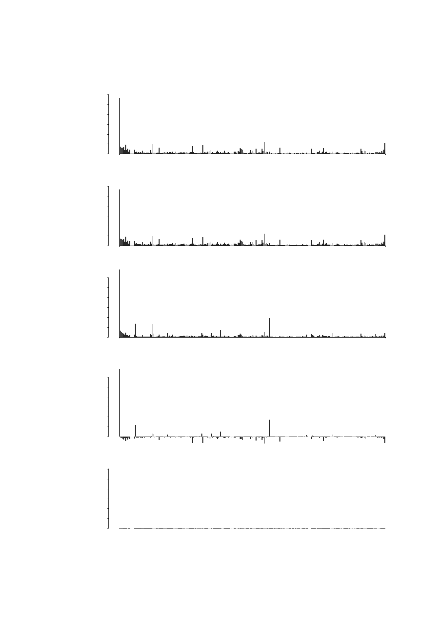
ngrams: 00,01,02,...,FE,FF

0.00

0.04

0.08

0.12

(a) Relative frequencies of n-grams created from benign files for n = 2 and s = 2.

ngrams: 00,01,02,...,FE,FF

0.00

0.04

0.08

0.12

(b) Relative frequencies of n-grams created from virus infected files for n = 2 and s = 2.

ngrams: 00,01,02,...,FE,FF

0.00

0.04

0.08

0.12

(c) Relative frequencies of n-grams created from virus loader files for n = 2 and s = 2. Note that the
relative frequency of n-gram “00” is cropped.

0.00

0.04

0.08

0.12

(d) Difference of relative frequency between benign files and virus loader files.

0.00

0.04

0.08

0.12

(e) Difference of relative frequency between benign files and virus infected files.

Fig. 4.

Relative frequencies of n-grams created from benign files, virus infected files

and virus loader files. Observe, that the relative frequencies of the n-grams created from
benign files and files infected are nearly indistinguishable. As a consequence, discrimi-
nating n-grams created from benign files and virus infected files is nearly infeasible.

Wyszukiwarka

Podobne podstrony:

więcej podobnych podstron