Modeling and Control of an Electric Arc Furnace

Benoit Boulet, Gino Lalli and Mark Ajersch

Centre for Intelligent Machines

McGill University

3480 University Street, Montréal, Québec, Canada H3A 2A7

Abstract
Electric arc furnaces (EAFs) are widely used in steelmaking and in
smelting of nonferrous metals. The EAF is the central process of
the so-called mini-mills, which produce steel mainly from scrap.
Typical EAFs operate at power levels from 10MW to 100MW.
The power level is directly related to production throughput, so it
is important to control the EAF at the highest possible average
power with a low variance to avoid breaker trips under current
surge conditions. For efficient power control, good dynamic
models of EAFs are required. This paper solves the electrical
circuit of an EAF with a floating neutral, proposes a dynamic
model for the EAF, and investigates simple proportional electrode
current and power control.

1 Introduction
Electric arc furnaces (EAFs) are widely used in steelmaking and in
smelting of nonferrous metals. The EAF is the central process of
the so-called mini-mills, which produce steel mainly from scrap.
Typical EAFs operate at power levels from 10MW to 100MW.
The power level is directly related to production throughput, so it
is important to control the EAF at the highest possible average
power with a low variance to avoid breaker trips under current
surge conditions. For efficient power control, good dynamic
models of EAFs are required [1].

2

Physical Model of Arc Furnace

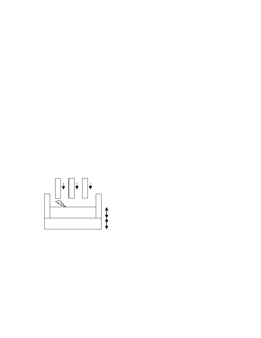
Figure 1 shows the physical model of the electric arc furnace. In
this particular EAF model, there are three electrodes that are
moved vertically up and down with hydraulic actuators. Each of
these electrodes has a diameter of roughly 1.5m, weighs
approximately 40 tons and is 1 to 2 stories tall. In theory, the ore
is melted with a huge power surge from the electrodes. The actual
product is denser than the scrap and thus falls to the bottom of the
furnace creating the matte. Above the matte lies the slag where the
electrode tips are dipped. The tremendous heat created by these
electrodes causes the ore to liquefy and separate. Thereupon more
raw materials are placed in the furnace and the process repeats
itself.

2.1 Arcing
Arcing is a phenomenon that occurs when the electrodes are
moved above the slag. As the electrode approaches the slag,
current begins to jump from the electrode to the slag, creating
electric arcs. Depending on the magnitude of the input voltages of
the electrodes, the arcing distance can vary. Usually, arcing occurs
in a region within centimeters of the slag (approximately 10-
15cm). Therefore, the EAF model must take into account the
instances when x

1

, x

2

, x

3

are negative (i.e. the electrodes are

suspended above the slag). Figure 1 above shows the sign
convention used in the project.

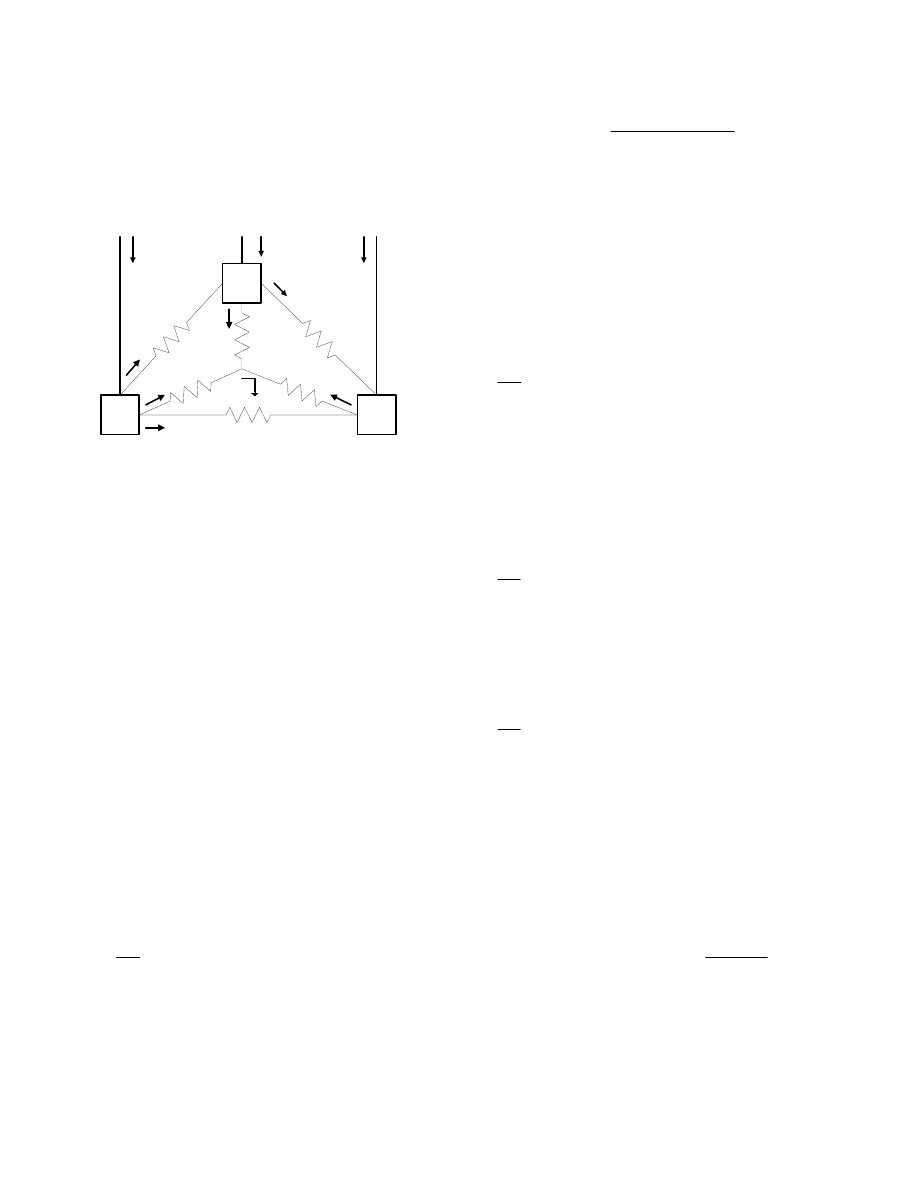
3

Solving the Electrical Circuit of the EAF

To solve any electrical model, assumptions are made to facilitate
the derivation. Similarly, the EAF electrical circuit requires
several assumptions before reaching the final equations. The first
step in the analysis of the electrical circuit is to use Kirchoff’s
Current Law (KCL) to equate currents and voltages. Figure 2
shows 4 nodes, one for each of the electrodes and the fourth
representing the virtual ground at the matte (V

m

). Using these

nodes, it is possible to determine the current in each electrode with
respect to each voltage and the conductance coefficients, using its
position as the input. Proper assumptions can facilitate derivations
thus calculating the following equation involving matrices:

[ ] [

][ ] [ ]

i

i

j

i

i

I

G

x

B

=

+

Equation 1: Current Matrix Model

Here, I

i

is a 3x1 matrix with electrode currents, G

ij

is a 3x3

conductance matrix and B

i

is a 3x1 constant matrix.

3.1

Assumptions

For the EAF circuit, several assumptions were made. It must be
noted that this is a three-phase circuit with a double configuration.
The outer resistances (inter-electrode resistances) form a delta-
circuit with the three nodes. The inner resistances (slag-to-matte
resistances) form a wye-connection with V

m

as a virtual ground

(floating neutral). Figure 2 shows the electrical model for the EAF
with the chosen direction of currents.

To simplify calculations, the inter-electrode resistances are
equivalent and represented by R. As for the slag-to-matte
resistances, tests showed that these resistances displayed inverse
linear relations with respect to their position. Consequently, by
taking the slag-to-matte conductances, the inverse function
becomes a linear relationship, which makes for simpler
calculations. The slag-to-matte conductances G

i

, where i

represents the electrode, can be written as:

i

i i

s

G

c x G

=

+

Equation 2: Slag-to-Matte Conductance

Figure 1:

Physical Model of EAF

MATTE

SLAG

1
m

3

2

AR

C

1

+ve X

-ve X

0-7803-7896-2/03/$17.00 ©2003 IEEE

3060

Proceedings of the American Control Conference

Denver, Colorado June 4-6, 2003

where c is the conductance coefficient (in Siemens/m), x

i

is the

immersion depth of the electrode in the slag (in m) and G

s

is the

total conductance of the slag (in S). In other words, G

s

is the

conductance of the slag when the electrodes are positioned at the
surface of the slag. Using these assumptions and KCL, it is now
possible to solve the EAF electrical circuit.

3.2 Nodal

Equations

The following sets of equations can be obtained by

applying KCL to each of the four nodes displayed in Figure 2.

1

12

1

2

1

1

13

1

3

(

)

(

)

(

)

m

I

G V

V

G V

V

G V

V

=

−

+

−

+

−

2

12

1

2

2

2

23

2

3

(

)

(

)

(

)

m

I

G V

V

G V

V

G V

V

= −

−

+

−

+

−

3

3

3

13

1

3

23

2

3

(

)

(

)

(

)

m

I

G V

V

G V

V

G V

V

=

−

−

−

+

−

1

1

2

2

3

3

(

)

(

)

(

) 0

m

m

m

G V

V

G V

V

G V

V

−

+

−

+

−

=

Equation 3: KCL using Conductances

Equation 4 represents the expression for V

m

, which will be used to

replace V

m

in the KCL equations above.

1 1

2 2

3 3

1

2

3

m

G V

G V

G V

V

G

G

G

+

+

=

+

+

Equation 4: Expression for V

m

3.3 Current

(I

I

) Calculations

Considering that the currents of the three electrodes will behave in
a similar manner, it is not necessary to display in full detail the
complete derivation for all three currents. The derivation of I

2

and

I

3

therefore follows from I

1

. The final expression for the total

current I

1

flowing through electrode 1 is shown in Eqn 5, with the

position inputs properly factored. I

1

is equal

to:

(

)

(

)

(

)

(

)

(

)

(

)

(

)

(

)

(

)

(

)

(

)

(

)

(

)

1 1

2 1

3 1

1 2 2

1

2

1

1 3 3

1

3

2

1 2

2 2

3 2

1

3

1 3

2 3

3 3

2

1

2

3

2

1

2

2

2

3

s

s

s

s

s

TOT

s

s

s

s

V c G

G

V c G

G

V c G

G

c c x V V

x

c c x V V

x V c G

G

V c G

G

V c G

I

G

x V c G

G

V c G V c G

G

V V

V

G

GG





+

−

+

−

+

+

−

















+

−













+

+

−

+

−

=









+

+

−

−

+









+

− −

+









Equation 5: Current in Electrode 1 (I

1

)

Similarly, Equations 6 and 7 represent the total currents

I

2

and

I

3

respectively.

(

)

(

)

(

)

(

)

(

)

(

)

(

)

(

)

(

)

(

)

(

)

(

)

(

)

1

1 1

2 1

3 1

1 2

2 2

3 3

2 3 3

2

3

2

1 2 1

2

1

2

3

1 3

2 3

3 3

2

1

2

3

2

2

1

2

2

3

s

s

s

s

s

TOT

s

s

s

s

x

V c G

G

V c G

G

V c G

V c G

G

V c G

G

V c G

G

c c x V

V

x

c c x V

V

I

G

x

V c G V c G

G

V c G

G

V

V

V

G

GG





−

+

+

+

−





−

+

+

+

−

+

+

−









+













+

−

=













+

−

−

+

−

+









+ − +

−

+









Equation 6: Current in Electrode 2 (I

2

)

(

)

(

(

(

)

(

)

(

)

(

)

(

)

(

)

(

)

(

)

(

)

(

)

































+

+

−

−













−

+

−

+

+

+

+

−

+

−

+

+

+

+

−

−

+

+2

G

))

−

−

+

−

=

s

s

s

s

s

s

s

s

s

TOT

GG

G

V

V

V

V

V

x

c

c

V

V

x

c

c

G

G

c

V

G

G

c

V

G

G

c

V

x

G

G

c

V

G

G

c

V

G

c

V

x

G

c

V

G

c

V

G

G

c

V

x

G

I

3

2

2

2

1

2

3

2

1

2

3

2

3

2

1

3

1

3

1

3

3

3

2

3

1

3

2

3

2

2

2

1

2

1

3

1

2

1

1

1

3

Equation 7: Current in Electrode 3 (I

3

)

where

1

1

2

2

3

3

3

TOT

s

G

c x

c x

c x

G

=

+

+

+

Equation 8 represents the Current Matrix Model shown by Eqn 1

(

)

(

)

(

)

(

)

(

)

(

)

(

)

(

)

(

)

(

)

(

)

(

)

(

)

1 1

2 1

1 3

2 3

1 2

2 2

3 1

1 2 2

1

2

3 2

3 3

1 3 3

1

3

1 2

2 2

1

1 1

2 1

2

3 3

3 1

3

2

2

2

2

2

1

s

s

s

s

s

s

s

s

s

s

s

TOT

V c G

G

V c G

G

V c G

G

V c G

V c G

G

V c G

G

V c G

G

c c x V

V

V c G

V c G

G

c c x V

V

V c G

G

V c G

G

I

V c G

G

V c G

G

I

V c

G

V c G

I

+

−

+





+

−

−





+

−

+









−

+

+

−

















−

+













+

−





−

+

+

+

 

−

+

+

+





 

=

−





 

−





 

 

(

)

(

)

(

)

(

)

(

)

(

)

(

)

(

)

(

)

(

)

(

)

(

)

(

)

(

)

1 3

2 3

2 3 3

2

3

3 3

1 2 1

2

1

1 3

2 3

1 1

2 1

1 2

2 2

3 3

1 3 1

3

1

3 1

3 2

2 3 2

3

2

2

2

2

2

s

s

s

s

s

s

s

s

s

s

V c G V c G

G

G

G

c c x V

V

V c G

G

c c x V

V

V c G

G

V c G

G

V c G

G

V c G

V c G V c G

G

V c G

G

c c x V

V

V c G

G

V c G

G

c c x V

V







−

−

+









+

+

−













−

+









+

−





−

+

−

+





−

+

−

−

−

+













+

+

+

−





















−

+

+

+













+

−





(

)

(

)

(

)

(

)

2

1

1

2

3

2

1

2

3

3

1

2

3

2

3

2

2

s

s

TOT

x

V

V

V

G

GG

x

V

V

V

G

x

V

V

V























−

−





 





+





 





+

− +

−





 









 

− −

+



  





























Equation 8: Electrode Current Equations in Matrix Form

Figure 2: Electrical Model of EAF

R

1

R

13

R

3

R

12

R

23

2

1

3

R

2

I

1

I

2

I

3

V

1

V

2

V

3

i

12

i

2m

i

1m

i

13

i

23

i

3m

V

m

i

m

= 0

3061

Proceedings of the American Control Conference

Denver, Colorado June 4-6, 2003

Note that, in Equation 8 above, the 3x3-conductance matrix is
nonlinear. Presence of terms containing x

1

, x

2

, and x

3

along the

main diagonal indicate this clearly. Therefore this system cannot
be controlled as a linear state-space model. Therefore,
linearization of the G

ij

conductance matrix will be necessary to

control this system with state feedback.

Another observation is that when the electrodes are positioned
flush on the slag (i.e. x

1

= x

2

= x

3

= 0), there is still a constant

current passing through them. This constant value is represented
by the second term of Equation 8. It arises from the presence of
G

s

in the slag-to-matte conductance.

4

Initial Model of EAF

Now that the EAF electrical circuit is solved, the next step is to
implement Equation 8 as an open-loop system to test different
cases for several electrode positions. For the output current
matrix I

i

, this conductance matrix G

ij

depends on the electrode

voltages (V

1

, V

2

and V

3

) and their respective conductance

coefficients (c

1

, c

2

and c

3

). Therefore, appropriate values have to

be calculated in order implement a realistic system. The chosen
values will be explained in the next sub-section.

In addition to setting-up the electrode voltages and conductance
coefficients, it is important to set the slag-to-matte conductance
offset G

s

and the inter-electrode conductance G. For each of

these variables there exists an acceptable range of values
capable of adequately modeling the system. Table 1 shows the
list of variables with their acceptable ranges and finally the
values chosen for simulation purposes.

Table 1: Constants

Variables

Acceptable

Range

Chosen Value

V

1

, V

2

and V

3

100-1000V

500V

c

1

, c

2

and c

3

1-100S/m

20

S/m

G

s

5-25S 10S

G

≈

0S

0.1S

Voltages used in the simulation are phasors with 500V
magnitude and 120

°

phase difference. Secondly, all values

follow SI units with meters as the length unit.

4.1 Matlab

Simulation

The Matlab™ simulations indicate the important values for
critical electrode positions. From these simulations, if the
electrodes are positioned on the slag, approximately 5kA of
constant current will pass through each of them, while
individually using about 2.5MW of power. When the electrodes
are completely immersed in the slag, a maximum of 15kA of
current is present while using a maximum of 7.5MW per
electrode. These simulations also indicate that drastic changes
in the position of the electrodes above the slag is less sensitive
for current and power as when they are immersed deep in the
slag.

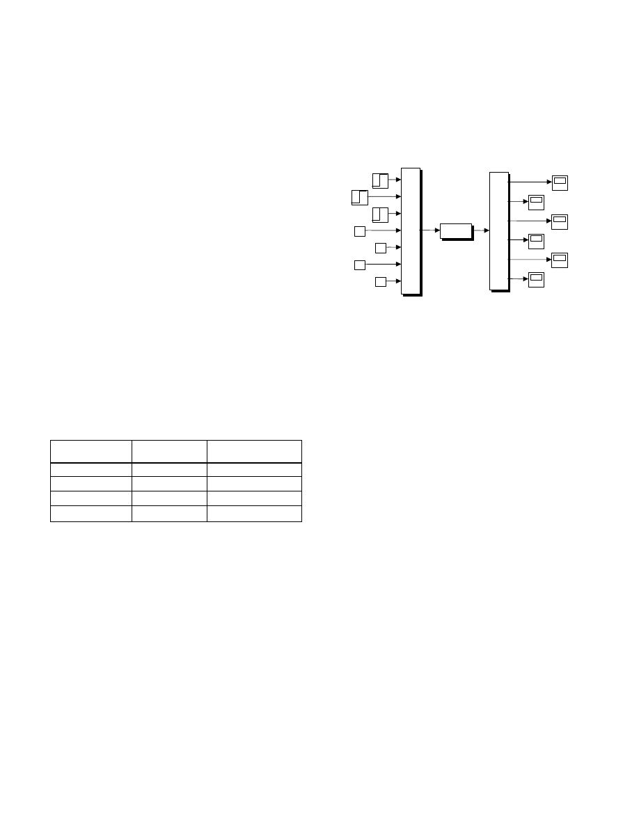
5 Open-Loop

Simulations

5.1

Simulink Block Diagram

Figure 3 represents the open-loop block diagram used in the
simulation of the EAF.

Figure 3: Simulink Open-Loop Block Diagram

As can be seen from Figure 3, there are 7 inputs and 6 outputs to
the Matlab function. The position of each electrode (x

1

, x

2

, and

x

3

) is represented by a step input. The voltages applied to each

electrode are represented by constants V

1

, V

2

and V

3

(their

phase representation is described within the Matlab code). The
last input is the inter-electrode conductance, set to 0.1S. The
outputs are the respective magnitudes of the currents (I

1

, I

2

, and

I

3

)

and power (P

1

, P

2

, and P

3

)

passing through each electrode.

5.2 Introducing

Noise

In any system, noise plays a prevalent part in altering the output
of the system. No system can be modeled efficiently without
taking noise into account. The EAF system is no exception. The
only difference here is that the noise will not be applied on the
input of the system, but rather on the output. The immense size
and weight of the electrodes make them immune to small
disturbances, and therefore any input noise will have minimal
effect on the output. Therefore, any noise affecting the system
will have to be introduced on the output side of the system.

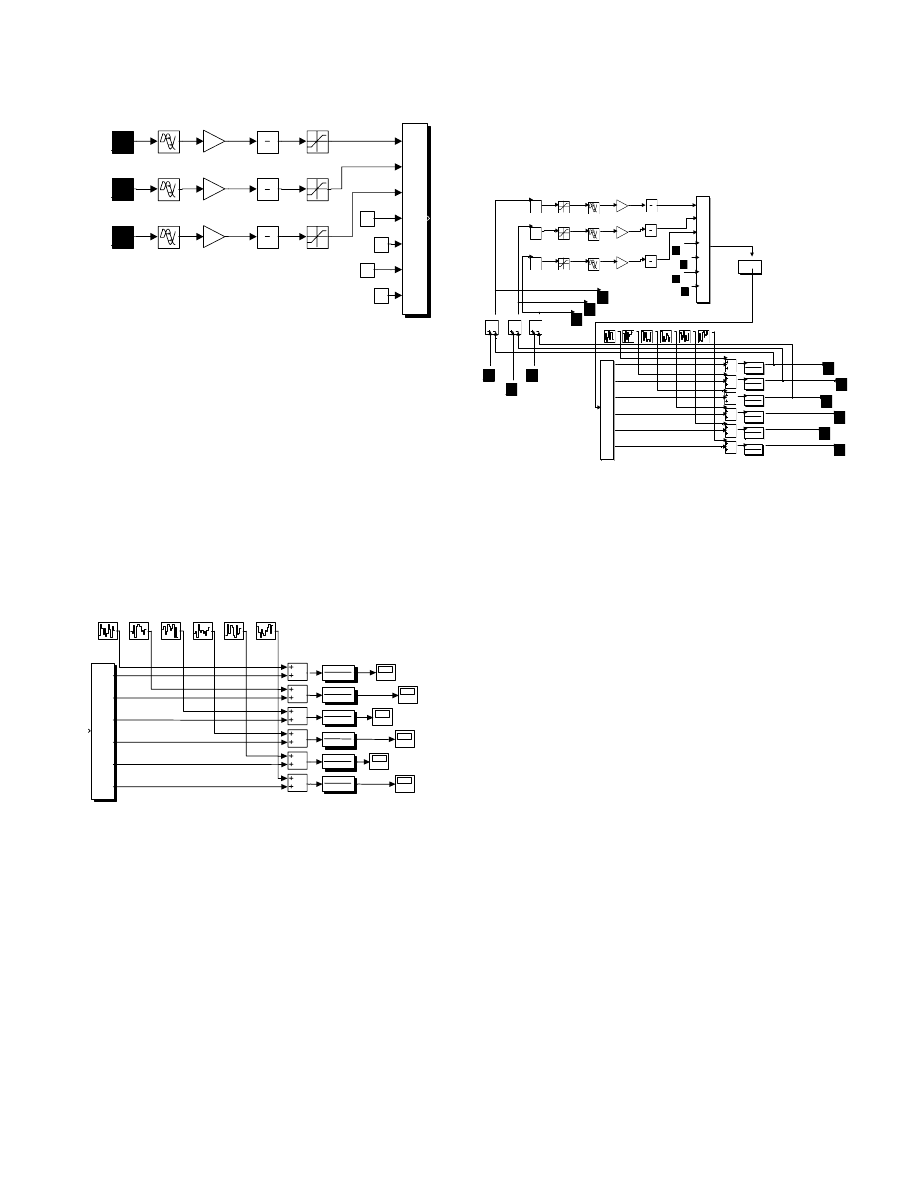
5.3 System

Dynamics

The next step in implementing a controller for the EAF system
is to include the system dynamics. Unfortunately, the position
step inputs do not realistically represent the inputs to a real-life
furnace. In real-life EAFs, hydraulic actuators control the
positions of the electrodes [2]. To simplify the physics of the
system, an assumption is made that the hydraulic cylinders are
powerful enough to neglect the mass of the electrodes.
Therefore, the model of the hydraulic system includes a one-
second time delay, followed by a gain (speed conversion), and
then an integrator. Figure 4 shows the input half of the open-
loop system with the proper modifications.

x3

x2

x1

m ag_p3

m ag_p2

m ag_p1

m ag_i3

m ag_i2

m ag_i1

M ATLAB

Function

conductance1

500

V3

500

V2

500

V1

Mux

Mux

0.1

G

Demux

Demux

3062

Proceedings of the American Control Conference

Denver, Colorado June 4-6, 2003

x3

x2

x1

0.1

m/sec/%

0.1

m/sec/%

0.1

m/sec/%

delay

delay

500

V3

500

V2

500

V1

Saturation

Saturation

Saturation

Mux

Mux

0.1

G

delay

s

1

s

1

s

1

Figure 4: Input Half of Open-Loop incl. System

Dynamics

In Figure 4, the input step responses now represent the valve
opening as a percentage. The one-second delay represents the
actual time it takes for the valves to open/close as desired. The
difference between Figures 3 and 4 is that the position of the
electrodes is now a function of the percentage valve openings.

Other nonlinear additions to the EAF system include sensors and
transducers. Transducers are represented in the system by first
order filters. The primary function of transducers however, is
not to filter the signal, but to translate the signal from a given
input signal to a signal that can be processed. These blocks are
placed after the noise in the output half of the open-loop system
and are represented by first-order transfer functions with a 25ms
time constant. Figure 5 shows the location of the transducers in
the system.

Figure 5: Output Half of Open-Loop with Noise

6

Control Principle

One of the main objectives of the three-electrode Electric Arc
Furnace simulator study is to have the electrodes maintain
constant power consumption. This is achieved by moving the
electrodes to a given depth, obtaining the desired resistances (or
conductances), which leads to a constant power consumption.
To attain this goal, the open-loop system described in the
previous section must be closed in order to create an error
signal. The control principle is accomplished by minimizing this
error signal with specific controllers. For this system, although
the power is to remain constant, since the power magnitudes are
scalar multiples of the electrode currents, controlling the current
will lead to power control as well.

6.1 Closed-Loop

System

Figure 6 shows the closed-loop system for the EAF.

Figure 6: Closed-Loop System

A feedback loop has now been added to the output of the open-
loop system. The output currents are fed back into the negative
port of an adder block, where they are combined with the initial
step responses representing the desired current. The difference
between the desired current and output current is then fed into a
PID controller set appropriately to transform a current
magnitude to a percent error. This percent error orders the
hydraulic actuators to open the valves such that a new resistance
sets the corresponding currents to converge to the desired
currents.

The saturation blocks at the top of Figure 6 are relocated
preceding the delay and integrator blocks and set to ensure that
the percent error never surpasses

±

100%. Initially, the step

response denoting the desired current is transmitted through the
system, activating the electrodes to move up or down. Once the
‘Matlab function’ block calculates the output current, it is
negated and added to the desired current. As the loop is
repeatedly executed, the difference between the currents
ultimately diminishes to zero and the objective of controlling the
power is achieved.

6.2

Setting the PID Controller

For preliminary testing, the PID controllers in Figure 6 are
fundamentally P controllers as the D-gain and I-gain are set to 0.
For the purpose of the EAF system, the P-gain had to transform
a current signal to a percent error. Thus the gain of the P-
controller was originally set to 0.001. However, the closed- loop
error took much too long to reach zero (under steady-state
conditions).

Therefore, the P controller gain had to be increased to speed up
the step response. After much tuning, setting the P-gain to
0.0045 gave the most satisfactory step response. The next sub-
section will display simulations with different desired currents.

mag_p3

mag_p2

mag_p1

mag_i3

mag_i2

mag_i1

1

0.025s+1

1

0.025s+1

1

0.025s+1

1

0.025s+1

1

0.025s+1

1

0.025s+1

Noise_P3

Noise_P2

Noise_P1

Noise_I3

Noise_I2

Noise_I1

Demux

Demux

mag_p3

mag_p2

mag_p1

mag_i3

mag_i2

mag_i1

err3

err2

err1

MATLAB
Function

conductance1

500

V3

500

V2

500

V1

Transport

Delay2

Transport

Delay1

Transport

Delay

1

0.025s+1

1

0.025s+1

1

0.025s+1

1

0.025s+1

1

0.025s+1

1

0.025s+1

Saturation5

Saturation4

Saturation3

PID

PID Controller2

PID

PID Controller1

PID

PID Controller

Noise_P3

Noise_P2

Noise_P1

Noise_I3

Noise_I2

Noise_I1

Mux

Mux

I3_des

I2_des

I1_des

0.0

Gain2

0.0

Gain1

0.0

Gain

0.1

G

Demux

Demux

s

1

s

1

s

1

3063

Proceedings of the American Control Conference

Denver, Colorado June 4-6, 2003

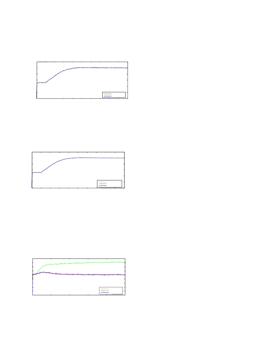
6.3 Closed-Loop

Simulations

The first simulation is performed when all the desired currents
are set to 10kA, the mean of maximum and minimum electrode
currents. Figure 7 represents the output currents. Note that the
currents of all electrodes are plotted on the same graph.

Figure 7: Closed-Loop Current Magnitudes (Desired

Currents = 10kA)

Figure 8 reveals the power magnitudes of the electrodes with the
same desired currents as above. As explained previously, the
power magnitudes are scalar multiples of the current
magnitudes. Hence, the desired power for each electrode is
5MW for a desired current of 10kA since the magnitude of the
voltage is 500V RMS.

Figure 8: Closed-Loop Power Magnitudes (Desired Power =

5MW)

Since the system model already contains an integrator (in order
to change electrode speed into electrode position), the effect of
adding an I-gain will be negligible. The next simulation involves
testing for coupling of the electrode currents. Figure 9 represents
the current magnitude for the case when I

1

= 10kA and I

2

= I

3

=

5kA. Having different desired currents when running a
simulation leads to coupling between the electrodes. This
phenomenon is explained by the nonlinear terms found in the
conductance matrix G

ij

.

Figure 9: Closed-Loop Current Magnitudes showing

Coupling

The consequences of coupling are that the currents have
different step responses. By virtue of these differences in error
responses, ideal PID controllers would have to monitor the
system such that each current attains its steady-state in the
fastest time possible. A future goal is to determine a decoupling
controller in order to combat these coupling effects.

7 Conclusion
The objectives of this study were clearly detailed from the
beginning. The EAF electrical circuit was successfully solved
and modeled in Matlab. The Matlab simulation determined the
system extremes for current flow and power consumption for
each electrode. The initial EAF block diagram was designed in
Simulink outputting individual current and power magnitudes.
Step functions were used for the electrode positions and the
Matlab code was transformed into a ‘Matlab Function’ block in
Simulink to perform the necessary calculations.

For a more realistic model of the EAF, the dynamics of the
system needed to be included. Hydraulic actuators, sensors and
transducers were all appropriately placed in Simulink open-loop
system to model electrode movement by valves and the
introduction of noise. Several simulations were executed and
plotted representing a wide range of electrode displacements.

Finally, a feedback loop was introduced to create a closed-loop
system. The input step functions now represent the desired
current to control the power. The current output was fed back
and subtracted from the desired current to form an error signal.
The error signal was transformed to a percent error by a PID
controller. All simulations demonstrated throughout the project
implemented a P-controller with a 0.0045 gain. Adding the
differentiator and integrator gains will improve the step
response. The coupling effects between electrodes were also
examined.

Future goals for the three-electrode arc furnace simulator study
include further testing for all coupling currents, the development
of optimal decoupling controllers, and linearizing the system in
order to implement a state-space controller. Analysis of many
parameters’ effects on the EAF model can also be included in
future objectives. These parameters can include the effect of the
reactances on the system’s power factor and the effect of arcing
as a function of temperature inside the furnace. Another
objective would be to see if the ideal PID-regulators for linear-
controlled electrodes would work in ‘bang-bang’ furnaces and if
not, find the relationship between the two types of furnaces.

8 References
[1] B. Boulet, V. Vaculik, G. Wong, Control of High-Power
Non-Ferrous Smelting Furnaces, IEEE Canadian Review,
summer 1997.

[2]

G. Dosa, A. Kepes, T. Ma and P. Fantin, Computer

control of high-power electric furnaces. Challenges in
Process Intensification Symposium, 35th Conference of
Metallurgists of the Metallurgical Society of CIM,
Montreal, Quebec, August 24-29, 1996.

1

2

3

4

5

6

7

8

9

10

0

2000

4000

6000

8000

10000

Time (sec)

C

urr

en

t (A

m

ps

)

Current vs Time with Delay and Noise

Mag I1

Mag I2

Mag I3

1

2

3

4

5

6

7

8

9

10

0

1

2

3

4

5

x 10

6

Time (sec)

P

owe

r (

W

a

tts

)

Power vs Time with Delay and Noise

Mag P1

Mag P2

Mag P3

0

5

10

15

20

25

0

1000

2000

3000

4000

5000

6000

7000

8000

9000

Time (sec)

Cu

rr

en

t (

A

m

p

s)

Current vs Time with Delay and Noise

Mag I1

Mag I2

Mag I3

3064

Proceedings of the American Control Conference

Denver, Colorado June 4-6, 2003